Analytical solutions for precipitation size distributions at steady-state

Abstract

Analytical solutions are derived for the steady-state size distributions of precipitating rain and snow particles assuming growth via collection of suspended cloud particles. Application of the Liouville equation to the transfer of precipitating mass through size bins in a “cascade” yields a characteristic gamma distribution with a “Marshall-Palmer” exponential tail with respect to particle diameter. For rain, the principle parameters controlling size distribution shape are cloud droplet liquid water path and cloud updraft speed. Stronger updrafts lead to greater concentrations of large precipitating drops and a peak in the size distribution. The solutions provide a means for relating size distributions measured in the air or on the ground to cloud bulk microphysical and dynamic properties.

1 Introduction

In a seminal study by Marshall and Palmer (1948), populations of drops collected on dyed filter paper revealed size distributions that follow the mathematical form $n_{D}=n_{D_{0}}\exp\left(-\lambda_{MP}D\right)$ where $n_{0}\sim 8\times 10^{3}$ m^-3 mm^-1, $n_{D}\Delta D$ is the concentration $n$ of rain drops of size $D$ within a bin of width $\Delta D$, and $\lambda_{MP}=d\ln n_{D}/dD$ is the slope parameter that would be obtained from a log-linear plot. It was shown experimentally that $\lambda_{MP}$ (in mm^-1) can be related to the rain rate (in mm hr^-1) through $\lambda_{MP}=4.1R^{-0.21}$. Theoretically, Villermaux and Bossa (2009) assumed simple mass balance and that drops have fallspeeds of $v\propto D^{1/2}$ to obtain $\lambda\propto R^{-2/9}$, an exponent remarkably close to the value of 0.21 obtained by Marshall and Palmer (1948). Subsequent work by Gunn and Marshall (1958) showed a similar exponential form for the size distributions of melted snow aggregates.

More detailed information is provided by using a gamma distribution of form

$$n_{D}=n_{0}D^{\mu}\exp\left(-\lambda D\right)$$ (1)

where the pre-factor exponent $\mu$ controls the numbers of smaller particle sizes. For the purposes of representing an ensemble averaged over sufficiently large timescales and spatial scales, this parameterized combination of a power-law and an exponential tail provides the essential ingredients for microwave remote sensing and cloud microphysical process algorithms (Bennartz and Petty 2001; Morrison and Milbrandt 2015).

With mathematical reasoning, $\mu$ and $\lambda$ can be related to the bulk properties of precipitation, such as the mean mass and precipitation flux diameter (Ulbrich 1983; Sekhon and Srivastava 1970; Mitchell 1991) and observations suggest that $\mu$ and $\lambda$ are nearly linearly related (McFarquhar et al. 2015). What has yet to be fully explained is why gamma or exponential distributions appear to describe precipitation distributions so well, or the underlying cloud physics controlling the values of $\mu$ and $\lambda$. The mathematical simplicity of Eq. 1 would seem to beg the question of whether there exists an equally simple derivation.

The most obvious approach to this problem is to explicitly simulate distribution evolution for such key processes as vapor diffusion, collection, and break-up (Srivastava 1971; List et al. 1987). Unfortunately, an analytical solution expressible in terms of the cloud physics at hand is not possible without assuming a priori some initial functional form for the distribution (Feingold et al. 1988). To get a sense for the difficulty of the problem, a single raindrop will have collected of order one million cloud droplets of order 10 $\mu$m diameter within a timescale of order 1000 s before it reaches of a size 1 mm diameter, implying a mean time between collisions of milliseconds. The conditions required for initiation of this super-exponential inflation of particle volume may be easily parameterized (Garrett 2012), but not the deterministic details of what ensues. Limiting the degrees of freedom to $n_{0}$, $\mu$ and $\lambda$ reduces complexity, but presumes a priori that a gamma function should apply (List et al. 1987; Mitchell 1991).

One way that a first principles equilibrium solution can be obtained is by maximizing the entropy of a particle ensemble subject to bulk constraints on the ensemble properties. Applying this approach, Wu and McFarquhar (2018) derived a generalized form of Eq. 1 that is $n_{D}=n_{0}D^{\mu}\exp\left(-\lambda D^{\beta}\right)$. Unfortunately, this mathematical method does not provide explicit guidance for the relevant ensemble constraint. For example, if the ensemble is constrained by total precipitation mass, as might seem quite reasonable, then $n_{D}=n_{0}D^{2}\exp\left(-\lambda D^{\beta}\right)$ where $\beta=3$ (Yano et al. 2016). However, the observed value of $\beta$ is 1 and not 3, a difference that would greatly affect predicted concentrations of large rain drops.

The goal here is to derive the statistical distributions of precipitation particles by treating the size distribution as an open system at steady-state, defined by a continual throughput of condensed mass in a “cascade” through size classes. The philosophy is similar to that that taken to derive the energy distribution of isotropic fluid turbulence with respect to the size of the eddies, where the underlying assumptions are only that the turbulent kinetic energy dissipation rate is independent of eddy size (Tennekes and Lumley 1972) and that this energy is lost at the smallest eddies where viscous forces balance inertial forces. With precipitation, the cascade is of matter rather than energy, and mass is removed gravitationally from the ensemble at all sizes and not just at the extreme.

2 Generalized size distribution slope

The start is to define a number concentration distribution of particles with respect to mass $n_{m}=dn/dm$ such that the number concentration of particles in a bin of width $\Delta m$ centered around $m$ is:

$$n\left(m-\Delta m/2,m+\Delta m/2\right)=\int_{m-\Delta m/2}^{m+\Delta m/2}n_{m}dm$$ (2)

The Liouville equation for the evolution of $n_{m}$ in time $t$ due to transfer along an arbitrary set of co-ordinates $\vec{x}$ is (Yano and Ouchtar 2017):

$$\frac{\partial n_{m}}{\partial t}=-\nabla\cdot\left(n_{m}\frac{d\vec{x}}{dt}\right)$$ (3)

Mathematically Eq. 3 is similar to the Eulerian continuity equation. However, $\vec{x}$ does not have to be restricted to spatial co-ordinates as it is in treatments of fluid transport of particles. Here, it is assumed that $\vec{x}=\left(m,z\right)$ where $z$ is a downward-pointing vertical co-ordinate, so that transport is in and out of size bins due to the combined effects of particle growth and vertical fallout. If horizontal spatial variability is ignored then:

$$\frac{\partial n_{m}}{\partial t}=-\frac{\partial}{\partial m}\left(n_{m}\frac{dm}{dt}\right)-\frac{\partial}{\partial z}\left(n_{m}\frac{dz}{dt}\right)$$ (4)

For particles sufficiently large that collection and precipitation dominate, Eq. 4 can be rewritten as:

$$\frac{\partial n_{m}}{\partial t}=\frac{\partial n_{m}}{\partial t}\bigg{|}_{coll}+\frac{\partial n_{m}}{\partial t}\bigg{|}_{precip}$$ (5)

So, dividing by $n_{m}$ , the dynamics can be expressed in terms of timescales $\tau=\left|1/\left(\partial\ln n_{m}/\partial t\right)\right|$

$$\frac{1}{\tau}=\frac{1}{\tau_{coll}}-\frac{1}{\tau_{precip}}$$ (6)

with the signs defined such that $\tau_{coll}$ is the timescale for net transfer of particle number into a size bin of mass $m$ and $\tau_{precip}$ is the timescale for removal.

Because precipitation is the primary mechanism by which particles are both collected and removed, $\tau_{coll}$ and $\tau_{precip}$ are related. Air currents in clouds are governed by turbulent vertical motions with their own characteristic eddy timescale $\tau_{turb}\sim 2\pi/N\sim 10^{3}\>{\rm s}$, where $N\sim 10^{-2}\>{\rm s^{-1}}$ is the saturated buoyancy frequency for cloud motion adjustments with respect to their stably stratified surroundings (Durran and Klemp 1982; Garrett et al. 2018). Here we assume the fallspeed of precipitation particles $v$ relative to the ground is independent of small scale updrafts and downdrafts in the inertial sub-range, permitting us to ignore non-equilibrium evolution over timescales and spatial scales that are less than $\tau_{turb}$ and $\tau_{turb}v$ respectively. In this case, and provided that no precipitation falls into the cloud through its top, the change in particle number due to settling of particles out the bottom of a vertically and horizontally uniform cloud layer of depth $H$ at terminal fallspeed $v$ in an updraft of speed $w$ is:

$$\frac{\partial n_{m}}{\partial t}\bigg{|}_{precip}=-\frac{\partial}{\partial z}\left(n_{m}\frac{dz}{dt}\right)\simeq-\frac{n_{m}\left(v-w\right)}{H}$$ (7)

With respect to collection, the total mass concentration flux along the mass co-ordinate due to collection of other cloud particles is:

$$\frac{\partial n_{m}}{\partial t}\bigg{|}_{coll}=-\frac{\partial}{\partial m}\left(n_{m}\frac{dm}{dt}\right)=-\frac{\partial}{\partial m}\left(n_{m}\rho_{cloud}v\sigma\right)$$ (8)

where $\rho_{cloud}=\int_{0}^{m_{c}}n_{m}dm$ is the population of cloud particles smaller than than critical mass $m_{c}$ with sufficiently small fall speeds to be collected by heavier particles that have collection cross-section $\sigma$ normal to the fall velocity. Note that collection is independent of $w$ if all particles are buoyed equally by an updraft.

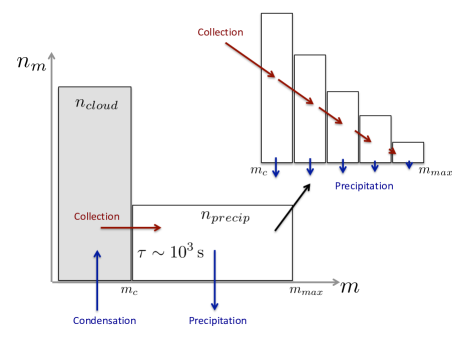
Figure 1: Illustration of precipitation distributions as an open system at steady-state, where the time scales for condensation, collection and precipitation are equal and net transfer of mass into precipitation size bins is balanced by fall-out.

Figure 1 illustrates the steady-state solution. For the size distribution to be stationary, such that $1/\tau\sim\partial\ln n_{m}/\partial t\simeq 0$, it follows from Eq. 6 that $\tau_{coll}\simeq\tau_{precip}$. Dividing Eq. 7 by $n_{m}$, and ignoring for the moment updrafts, then $\tau_{precip}\sim H/v$. Very roughly, for a small drop $\sim 1$ mm diameter that falls towards the ground at speed $v\sim 1$ m s^-1 through a cloud of depth $H\sim 1000$ m, the removal timescale is $\tau_{precip}\sim 10^{3}$ s. From Eq. 8, collisions transfer mass into larger size bins with timescale $\tau_{coll}\sim m/\left(\rho_{cloud}v\sigma\right)$. For the the same small drop in a cloud with liquid water content $\rho_{cloud}\sim 10^{-3}$ kg m^-3, $m\sim 1\times 10^{-6}$ kg and $\sigma\sim 10^{-6}$ m², then $\tau_{coll}\sim 10^{3}$ s, which is similar to $\tau_{precip}$.

A similar value of $\tau_{coll}$ is obtained for a $\sim 0.1$ mm diameter drop. Moreover, the $\sim 10^{3}$ s timescale is similar to the period of turbulent oscillations in clouds $\tau_{turb}$ that would be associated with the production of condensate, implying a timescale $\tau_{cond}$ that is also $\sim 10^{3}$ s. Of course, crude scale analysis lacks the details of precipitation production by clouds. Nonetheless, it serves to illustrate an open system at steady-state defined by a continuous throughput of condensed mass at rate $dM/dt\sim mn_{m}/\tau_{coll}$. The rate of mass production of suspended droplets roughly equals the rate of conversion to larger precipitating particles, and the eventual loss of these particles by gravity.

The functional form of a stationary precipitation size distribution can be arrived at by substituting Eqs. 7 and 8 into Eq. 4:

$$\frac{\partial}{\partial m}\left(n_{m}\rho_{cloud}v\sigma\right)=-\frac{n_{m}\left(v-w\right)}{H}$$ (9)

Then, dividing by Eq. 8 and noting that cloud mode particles are by definition less massive than precipitation mode particles, in which case $m_{c}<m$ and $\partial\ln\rho_{cloud}/\partial m=0$:

$$\partial\ln\left(n_{m}v\sigma\right)=-\frac{\left(1-w/v\right)}{\rho_{cloud}\sigma H}\partial m$$ (10)

Integrating across the precipitation size distribution from $m_{c}$ to $m$:

$$n_{m}v\sigma=n_{m_{c}}v_{m_{c}}\sigma_{m_{c}}\exp\left[-\frac{\int_{m_{c}}^{m}\left(1-w/v\right)dm/\sigma}{\rho_{cloud}H}\right]$$ (11)

For physical interpretation, Eq. 11 represents the number flux of particles through mass bins due to collection at rate $j_{m}=n_{m}v\sigma$. With some rearranging, it can be shown that Eq. 11 is equivalent to $j_{m}=j_{m_{c}}\exp\left(-\tau_{coll}/\tau_{precip}\right)$. As precipitation particles grow by collection to larger values of $m$, there is a progressive decrease in the number of precipitation particles that remain to grow to the next size bin. Statistically speaking, the population of particles with the longest journey has had the greatest exposure to predation from precipitation during the period it resided in all smaller bins. If $\tau_{coll}/\tau_{precip}\gg 1$, then the particle concentration must be correspondingly small.

Snow and rain particles can be highly deformed from sphericity (Villermaux and Bossa 2009). Parameterized power-laws that provide numerical fits relating $m$ to $\sigma$ and $D$ abound in the literature (Locatelli and Hobbs 1974; Mitchell 1996). However, the exponent in Eq. 11 must be dimensionless, imposing the requirement that $m/\sigma$ have units of mass per unit area. To obtain the size distribution $n_{D}$, expressed with respect to diameter $D$, we assume the following general forms

$$\sigma=\pi D^{2}/4$$ (12)

$$m=\pi\rho_{e}D^{3}/6$$ (13)

where $D$ is a cross-section effective diameter given by Eq. 12 (Locatelli and Hobbs 1974). The effective density $\rho_{e}$ is defined to satisfy the spherical relationship between $D$ and $m$ for the case that $D$ refers to unmelted particles. If $\sigma$ is considered to be a collection cross-section, the efficiency of collection by one drop of another is implicit in Eq 12.

Substituting Eqs. 12 and 13 in Eq. 10, along with the transformation $dm=\pi\rho_{e}D^{2}dD/2$ assuming $\rho_{e}\neq\rho_{e}\left(D\right)$, the following general solution is obtained that expresses the slope of the size distribution with respect to $D$ on a log-linear plot:

$$\frac{\partial\ln n_{D}}{\partial D}=-\frac{d\ln v}{dD}-\left({1-\chi}\right){\lambda}$$ (14)

where

$$\chi=\frac{w}{v}$$ (15)

expresses the relative strength of the updraft velocity and

$$\lambda=\frac{2}{H}\frac{\rho_{e}}{\rho_{cloud}}$$ (16)

is the slope parameter that yields the Marshall-Palmer distribution in the limit that $\chi\rightarrow 0$ and $v\neq v\left(D\right)$. In terms of the cloud equivalent liquid water path $L=\rho_{cloud}H/\rho_{l}$ where $\rho_{l}$ is the bulk density of liquid water:

$$\lambda=\frac{2}{L}\frac{\rho_{e}}{\rho_{l}}$$ (17)

3 Solutions for number concentration distributions

If the terminal velocity of a precipitation particle in still air is expressed as a power-law:

$$v=aD^{b}$$ (18)

then Eq. 14 leads to:

$$\frac{d\ln n_{D}}{dD}=-\frac{b}{D}-(1-\frac{w}{aD^{b}})\lambda$$ (19)

A solution to Eq. 19 is complicated by the functional dependence of $b$ on $D$ (Beard 1976). However, if $b$ is assumed to be a non-unity constant, then the solution mathematically resembles a gamma distribution. Integrating Eq. 19 from $D_{c}\left(m_{c}\right)$ to $D$ yields

$$n_{D}=n_{D_{0}}\left(\frac{D}{D_{c}}\right)^{-b}\exp\left[-\lambda D\left(1-\frac{\chi}{\left(1-b\right)}\right)\right]$$ (20)

where $n_{D_{0}}=n_{D_{c}}\exp\left[\lambda D_{c}\left(1-\chi/\left(1-b\right)\right)\right]$. Eq. 20 becomes a gamma distribution for the limiting case that $\chi\rightarrow 0$. A positive exponential dependence on $D$ is obtained if $w>\left(1-b\right)v$.

If $b=1$, as applies to the intermediate fallspeed regime typical of drizzle for which $0.08\>{\rm mm}<D<1.2\>{\rm mm}$, $\rho_{e}=\rho_{l}$, and $a\simeq 4\times 10^{3}\>{\rm s^{-1}}$, then integrating Eq. 19 from $D_{c}\left(m_{c}\right)$ to $D$ yields the gamma distribution:

$$n_{D}=n_{D_{0}}\left(D/D_{c}\right)^{\mu}\exp\left(-\lambda D\right)$$ (21)

where

$$\mu=\lambda w/a-1=\frac{2w}{aL}-1$$ (22)

and $n_{D_{0}}=n_{D_{c}}\exp\left(\lambda D_{c}\right)$. Eq. 22 is qualitatively consistent with the roughly linear relationship between $\mu$ and $\lambda$ that has been noted for arctic clouds (McFarquhar et al. 2015). If $D_{c}$ is sufficiently close to the intercept at 0 that $\lambda D_{c}\ll 1$, or $\mu=0$, then all possible curves converge on $n_{D_{0}}\simeq n_{D_{c}}$, consistent with observations by Marshall and Palmer (1948). In the limit $w\rightarrow 0$, the power-law pre-factor $\left(D/D_{c}\right)$ has an exponent $\mu=-1$.

If the pre-factor exponent $\mu$ in Eq. 22 is positive, then there is a peak in the gamma-distribution, requiring that $\lambda w>4\times 10^{3}\>{\rm s^{-1}}$ or, by substituting Eq. 17, $w/L>2\times 10^{3}\>{\rm s^{-1}}$. In this case, the transition size $D_{t}$ representing the diameter of the peak is obtained by setting the slope function Eq. 21 to zero:

$$D_{t}=\mu/\lambda$$ (23)

Substituting Eq. 17 in Eq. 23 for the case that $\rho_{e}=\rho_{l}$ yields

$$D_{t}=w/a-L/2$$ (24)

where $w$ has units of mm s^-1.

Strictly, Eq. 21 only holds for smaller rain drops in the intermediate fallspeed regime where $b=1$. Extending it to larger drops as a rough approximation, Eq. 24 provides a simple guide for relating the shape of the size distribution, cloud dynamics, and the cloud water path. A precipitation size distribution characterized by a peak with $D_{t}>0$ can be expected to be observed in measurements of rain that falls from clouds with sufficiently high updrafts that $w/L>2a=8\times 10^{3}\>{\rm s^{-1}}$. For example, in a convective cloud with $L>1$ mm, this would translate to precipitation forming in an updraft of at least 8 m s^-1 with a relatively shallow slope parameter of $\lambda>$2 mm^-1.

An alternative simplification for integrating Eq. 14 is to assume a constant particle fall speed. Substituting $b=0$ into Eq. 20, the solution is the Marshall-Palmer distribution:

$$n_{D}=n_{D_{R}}\exp\left[-\lambda_{eff}D\right]$$ (25)

where

$$\lambda_{eff}=\left(1-\chi\right)\lambda$$ (26)

and $\lambda$ is related to the cloud water path through Eq. 17. Eq. 25 holds in the limit of small perturbations about a reference diameter $D_{R}$ assuming the fallspeed does not deviate significantly from $v\left(D_{R}\right)$. A judicious reference diameter choice for the exponential tail might be the median diameter $D_{f}$ of the precipitation mass flux $n_{D}m\left(v-w\right)$ .

One implication of Eq. 26 is that the measured size distribution depends on where it is sampled. For example, if precipitation distributions were to be measured in a cloud with radar, or aboard an aircraft, then it might be expected that the effective slope parameter $\lambda_{eff}$ would be negative for those particles with $v<w$, meaning that concentrations increase with size. Such particles would not be expected to reach the ground. Only those with $v>w$ could be measured requiring that $\lambda_{eff}>0$ for the entire distribution, closer to the results obtained by Marshall and Palmer (1948). A possible counter-example is precipitation distributions that initially formed in a strong updraft, and then only fell after the updraft decayed.

Effectively, the mathematical solutions provided here assume a priori conditions for a materially open system that is at steady-state. They ignore any disequilibria in fluxes in and out of size bins that might occur over timescales shorter than $\tau\sim 1000\,\rm{s}$, or over long timescales where slow meteorological changes affect the evolution of $w$ or $H$. Over intermediate timescales, they are most obviously suited for stratiform precipitation, although they could also apply to more dynamic convective precipitation provided averaging over a sufficient amount of time and space to smooth out non-equilibrium variability. Perturbation solutions might then be found for the case that $w$ and $H$ vary.

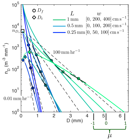
Figure 2: Rain size distributions obtained by integrating Eq. 19 subject to the observationally derived constraint that $n_{D_{0}}=6\times 10^{3}\exp\left(-3.2\mu\right)$ (Ulbrich 1983). Curves are grouped by three values of liquid water path $L$, and three values of the pre-factor exponent $\mu$. The corresponding value of $w$ is obtained from Eq. 22. Black dashed lines represent the Marshall-Palmer distribution for rain rates ranging from 0.01 mm hr^-1 increasing by orders of magnitude to 100 mm hr^-1. Diamonds represent $D_{t}>0$ and circles $D_{f}$ for each respective curve. Thin colored lines correspond to drop sizes for which $v<w$ that would be expected not to precipitate and thin black lines represent $\lambda_{eff}\left(D_{f}\right)$ as given by Eq. 26.

Figure 2 shows hypothetical curves for precipitation size distributions obtained numerically by integrating Eq. 19 for the case that $v$ is a continuous function of $D$, starting from a critical diameter $D_{c}=0.04$ mm. In general, larger values of $L$ are associated with greater concentrations of large droplets and higher rain rates. For $\mu=0$, the size distribution approximates a pure exponential with an intercept at $n_{D_{0}}=6\times 10^{3}$ (Ulbrich 1983). For $\mu=-1$ corresponding with zero updraft velocity, the size distribution is a negative power-law for small drop sizes. High updraft scenarios with $\mu=1$ exhibit shallower slopes in the tail of the size distribution and a peak in the distribution that agrees well with the expression for $D_{t}$ given by Eq. 24. Values of $\lambda_{eff}$ for the constant fallspeed assumption $v=v\left(D_{f}\right)$ (Eq. 26) match well with the local slope at $D_{f}$. High updraft speeds correspond with lower values of $\lambda_{eff}$. Values of $\lambda_{eff}$ are negative only for small values of $D$ for which $v<w$.

4 Discussion

This study did not address the impacts of turbulence on settling speed (Wang and Maxey 1993; Garrett and Yuter 2014), or that fragmentation of drops might produce significant numbers of particles with super-terminal fallspeeds (Montero-Martínez et al. 2009). Fragmentation has also been invoked as an explanation for the observed exponential tail (Marshall and Palmer 1948; Langmuir 1948). In support of of this hypothesis, laboratory and theoretical work by Villermaux and Bossa (2009) has shown that fragmentation of large drops $\sim 6\>{\rm mm}$ exiting near cloud base can reproduce the Marshall-Palmer distribution. The fragmentation timescale of these large drops $\tau_{burst}$ is of order $10^{-2}$ s, five orders of magnitude faster than $\tau_{coll}$. Thus, fragmentation cannot account for a steady-state solution as there is no known cloud process that could replenish 6 mm drops over timescales as short as $\tau_{burst}$. Additionally, such large drops are exceedingly rare in all but heavy precipitation. Recent photographic observations support collisions rather than breakup as being the primary determinant of the size distribution (Testik and Rahman 2016, 2017).

An additional limitation of the solutions described here is that they do not provide an explanation for the value of $n_{D_{c}}\simeq n_{D_{0}}$. It was assumed here without explicit justification that collection only applies to drops with critical diameters $D_{c}$ greater than 0.04 mm. It is often assumed that only drops with this size or larger have sufficiently high collection efficiencies (Pruppacher and Klett 1997). Alternatively, the 0.04 mm size threshold represents a switch from slowing growth rates during vapor condensation to accelerating growth rates by rapid “discovery” of new sources of liquid water during collection (Lamb and Verlinde 2011; Garrett 2012).

5 Summary

The mass continuity equation was applied to a horizontally and vertically uniform cloud layer to derive the size distribution of precipitation particles that exit its base, making the equilibrium assumption that convergence of mass within a size bin due to collection is balanced by fallout due to precipitation. The steady-state condition yields solutions for the slope of the number distribution with respect to particle diameter. Applying simplifying assumptions for the dependence of fallspeed on size, the precise shape of the distribution can be related analytically to the cloud liquid water path $L$ and the ratio of the updraft velocity to the cloud liquid water path $w/L$. High concentrations of large drops are related to high values of $L$ and $w/L$. If $w/L$ is sufficiently large, the local slope in the size-distribution is positive at small drop sizes and there exists a peak in the size distribution.

Calculations and measurements by Ulbrich (1983) and Marshall and Palmer (1948) suggest that $R\propto\lambda_{eff}^{-4.67}$. Eq. 25 for $\lambda_{eff}$ implies that rain-rates are highest coming from clouds with strong updrafts and high liquid water paths of suspended cloud droplets. While updraft velocities can be inferred from Doppler radar, an unfortunate limitation of existing ground-based remote sensing techniques for measuring cloud liquid water path is that they measure total liquid water path including precipitation and that the sensors fail when wetted by rain (Cadeddu 2012).

Thus, the results presented here present a basis for the theoretical prediction of relationships between precipitation microphysics, clouds and cloud dynamics. The focus was rain, however it is straight-forward to extend the results to snow provided the size distribution considered is with respect to melted snow particles as in Gunn and Marshall (1958) or that a suitable estimate is provided for snow density $\rho_{e}$ in Eq. 17 (Tiira et al. 2016). Further work is required to elucidate perturbation solutions for precipitation events that are not in steady-state.