Determining the Superconducting Transition Temperatures of Liquids

Abstract

We develop a non-perturbative approach for calculating the superconducting transition temperatures ($T_{\mathrm{c}}$’s) of liquids. The electron-electron scattering amplitude induced by electron-phonon coupling (EPC), from which an effective pairing interaction can be inferred, is related to the fluctuation of the $T$-matrix of electron scattering induced by ions. By applying the relation, EPC parameters can be extracted from a path-integral molecular dynamics simulation. For determining $T_{\mathrm{c}}$, the linearized Eliashberg equations are re-established non-perturbatively. We apply the approach to estimate $T_{\mathrm{c}}$’s of metallic hydrogen liquids. It indicates that metallic hydrogen liquids in the pressure regime from $0.5$ to $1.5\mathrm{\,TPa}$ have $T_{\mathrm{c}}$’s well above their melting temperatures, therefore are superconducting liquids.

I Introduction

Mercury, the only metallic element which is a liquid under the ambient conditions, happens to be the first superconductor ever discovered. At a superconducting transition temperature ($T_{\mathrm{c}}$) of $4.1\,\mathrm{K}$, however, it is frozen long before entering into the superconducting state. As a matter of fact, all superconductors discovered so far are solids. It seems improbable to find a superconducting liquid. Recently, the possibility emerges with the report of a possible observation of the Wigner-Huntington transition to metallic hydrogen (Dias and Silvera, 2017). Theoretically, it is predicted that hydrogen forms an atomic metal (McMahon et al., 2012) and has a relatively low melting temperature in the pressure regime from $0.5$ to $1.5\,\mathrm{TPa}$ (Chen et al., 2013; Geng et al., 2015). On the other hand, $T_{\mathrm{c}}$ predicted for the solid phase of metallic hydrogen is much higher than the melting temperature (McMahon and Ceperley, 2011). It raises an intriguing question: can a metallic hydrogen liquid be superconducting?

A theoretical answer to the question would require developing a formalism for predicting $T_{\mathrm{c}}$’s of liquids. For metallic hydrogen liquids, Jaffe and Ashcroft present an estimate of $T_{\mathrm{c}}$ in the density range within $1.2\leq r_{\mathrm{s}}\leq 1.6$ (Jaffe and Ashcroft, 1981), where $r_{\mathrm{s}}\equiv(3/4\pi n_{\mathrm{e}})^{1/3}/a_{\mathrm{B}}$ is the dimensionless density parameter with $n_{\mathrm{e}}$ being the electron density and $a_{\mathrm{B}}$ the Bohr radius. The density range is now believed not in the regime forming the atomic metal (McMahon et al., 2012). Their formalism is based on a heuristic generalization of the conventional electron-phonon coupling (EPC) theory (Grimvall, 1981; Giustino, 2017), which is developed specifically for ordinary solids, relies on the harmonic approximation of ionic motions, and is perturbative by nature. For liquids, however, the harmonic approximation breaks down and there is no apparent small parameter to facilitate a perturbative treatment. The applicability of the conventional EPC theory is therefore questionable.

It is desirable to build the EPC theory on a firmer ground, and seek for a formalism with applicability extendable to liquids and other unconventional systems such as anharmonic solids (Borinaga et al., 2016; Errea et al., 2013). With the advances of modern computation techniques, e.g., the ab initio path-integral molecular dynamics (PIMD) methods (Marx and Parrinello, 1996; Craig and Manolopoulos, 2004), we are now at a much better position for applying such a formalism and updating the calculation of metallic hydrogen liquids. More intriguingly, the development would also give rise to a prospect of searching for high-$T_{\mathrm{c}}$ EPC superconductors in unconventional systems.

In this paper, we develop a non-perturbative approach for calculating $T_{\mathrm{c}}$’s of liquids. The central ingredient of our approach is an exact relation between the electron-electron scattering amplitude induced by EPC and the fluctuation of the $T$-matrix of electron scattering induced by ions. The fluctuation can be evaluated with a PIMD simulation, and an effective pairing interaction can be inferred from the scattering amplitude. Our approach thus enables the evaluation of EPC parameters from first principles for liquids. For determining $T_{\mathrm{c}}$, we re-derive the Eliashberg equations in a non-perturbative context. The approach is applied to investigate the superconductivity of the liquid phase of metallic hydrogen. We find that metallic hydrogen liquids in the pressure regime from $0.5$ to $1.5\mathrm{\,TPa}$ have $T_{\mathrm{c}}$’s well above their melting temperatures, therefore are superconducting liquids.

The remainder of the paper is organized as follows. In Sec. II, we develop the theory of the superconductivity in liquids and general systems. Main theoretical results are summarized in Sec. II.1, and the proofs of these results are discussed in subsequent subsections. Based on the theory, a numerical implementation for metallic hydrogen is detailed in Sec. III, with main results summarized in Sec. III.3. Finally, Sec. IV is a summary.

II Theory

II.1 Summary of Main Results

In this subsection, we summarize the main theoretical results of this paper. They form the theoretical basis of calculating $T_{\mathrm{c}}$’s of liquids. The proof of these results are presented in subsequent subsections.

II.1.1 Notations

In our formalism, we define two kinds of single-particle Green’s functions for electrons. $\mathcal{G}\left[\bm{R}(\tau)\right]$ is the Green’s function of an electron system subjected to the ionic field with respect to a given ion configuration (trajectory) $\bm{R}(\tau)$:

$$\mathcal{G}\left[\bm{R}(\tau)\right]\left(\bm{r}\tau,\bm{r}^{\prime}\tau^{\prime}\right)=\\ -\mathrm{Tr}\left\{\hat{T}_{\tau}\left[\hat{\rho}_{\mathrm{ei}}\left[\bm{R}(\tau)\right]\hat{\psi}_{\sigma}(\bm{r}\tau)\hat{\psi}_{\sigma}^{\dagger}(\bm{r}^{\prime}\tau^{\prime})\right]\right\},$$ (1)

where $\bm{R}(\tau)\equiv\left\{\bm{R}_{i}(\tau),i=1\dots N_{\mathrm{i}}\right\}$ is the short-hand notation of the trajectories of $N_{\mathrm{i}}$ ions with $\tau\in[0,\hbar\beta)$, $\beta\equiv 1/k_{\mathrm{B}}T$ being the imaginary time arising in the Matsubara representation (Fetter and Walecka, 2003; Mahan, 2000), $\hat{\psi}_{\sigma}(\bm{r}\tau)$ and $\hat{\psi}_{\sigma}^{\dagger}(\bm{r}^{\prime}\tau^{\prime})$ are electron field operators, $\hat{\rho}_{\mathrm{ei}}\equiv Z_{\mathrm{ei}}^{-1}\hat{T}_{\tau}\exp[-(1/\hbar)\int_{0}^{\hbar\beta}d\tau(\hat{K}_{\mathrm{e}}+\hat{V}_{\mathrm{ei}}(\tau))]$ denotes the effective density matrix of the electron system with a grand-canonical Hamiltonian $\hat{K}_{\mathrm{e}}$ and subjected to a $\tau$-dependent ionic field $\hat{V}_{\mathrm{ei}}(\tau)$. See Sec. II.2.2 for details. Due to the presence of $\hat{V}_{\mathrm{ei}}(\tau)$ which breaks both the spatial and temporal translational symmetries, the Green’s function is in general not a function of ($\bm{r}-\bm{r}^{\prime}$, $\tau-\tau^{\prime}$).

The physical Green’s function, which is denoted as $\bar{\mathcal{G}}$, is obtained from $\mathcal{G}\left[\bm{R}(\tau)\right]$ after an ensemble average over ion trajectories. See Sec. II.2.2 for the definition of the ensemble average. For liquids, both the spatial and the temporal translational symmetries are recovered after the average. As a result, $\bar{\mathcal{G}}$ is a function of ($\bm{r}-\bm{r}^{\prime}$, $\tau-\tau^{\prime}$). We define its Fourier transform as

$$\bar{\mathcal{G}}\left(\omega_{n},\bm{k}\right)=\\ \int\mathrm{d}\tau\int\mathrm{d}\bm{r}e^{\mathrm{i}\omega_{n}(\tau-\tau^{\prime})-\mathrm{i}\bm{k}\cdot(\bm{r}-\bm{r}^{\prime})}\bar{\mathcal{G}}\left(\bm{r}-\bm{r}^{\prime},\tau-\tau^{\prime}\right),$$ (2)

where $\omega_{n}\equiv(2n+1)\pi/\hbar\beta$, $n\in Z$ is a Fermionic Matsubara frequency and $\bm{k}$ is a wave-vector. Note that we distinguish a function from its Fourier transform by their arguments [i.e., $(\bm{r}-\bm{r}^{\prime},\tau-\tau^{\prime})$ vs. $(\omega_{n},\bm{k})$].

We adopt an abbreviated matrix notation for presenting our formalism. A hatted symbol, e.g., $\hat{\mathcal{T}}$ in Eq. (6), denotes a matrix, while $\mathcal{T}_{11^{\prime}}$ in Eq. (5) denotes an element of the matrix. The indices of matrix elements are denoted by (decorated) numbers (e.g., $1$, $1^{\prime}$ or $\bar{1}$) instead of usual alphabets. The indices refer to the set of parameters labeling the basis of the matrix. We choose the basis in a particular way such that the average (physical) Green’s function $\bar{\mathcal{G}}$ is diagonal, i.e., $\left[\bar{\mathcal{G}}\right]_{11^{\prime}}=\bar{\mathcal{G}}_{1}\delta_{11^{\prime}}$. For liquids, the index $1$ refers to a Matsubara frequency-wave vector pair $(\omega_{n},\bm{k})$, and $1^{\prime}$ to $(\omega_{n^{\prime}},\bm{k}^{\prime})$, and $\bar{\mathcal{G}}_{1}\equiv\bar{\mathcal{G}}\left(\omega_{n},\bm{k}\right)$, $\delta_{11^{\prime}}\equiv\delta_{\omega_{n},\omega_{n^{\prime}}}\delta_{\bm{k},\bm{k}^{\prime}}$.

For liquids, which have both the temporal and the spatial translational symmetries, the basis is just the plane-wave function $\varphi_{\omega_{n}\bm{k}}(\bm{r}\tau)=(\hbar\beta V)^{-1/2}\exp\left(-\mathrm{i}\omega_{n}\tau+\mathrm{i}\bm{k}\cdot\bm{r}\right)$, where $V$ is the total volume of the system. In this case, matrix indices refer to the pair of $(\omega_{n},\bm{k})$. With the notation, a matrix element $\mathcal{T}(\bm{r}\tau,\bm{r}^{\prime}\tau^{\prime})\equiv\braket{\bm{r}\tau}{\hat{\mathcal{T}}}{\bm{r}^{\prime}\tau^{\prime}}$ can be expressed as:

$$\mathcal{T}(\bm{r}\tau,\bm{r}^{\prime}\tau^{\prime}) =\sum_{\omega_{n},\omega_{n^{\prime}},\bm{k},\bm{k}^{\prime}}\mathcal{T}_{\omega_{n}\bm{k},\omega_{n^{\prime}}\bm{k}^{\prime}}\varphi_{\omega_{n}\bm{k}}(\bm{r}\tau)\varphi_{\omega_{n^{\prime}}\bm{k}^{\prime}}^{\ast}(\bm{r}^{\prime}\tau^{\prime})$$

$$\equiv\sum_{11^{\prime}}\mathcal{T}_{11^{\prime}}\varphi_{1}(\bm{r}\tau)\varphi_{1^{\prime}}^{\ast}(\bm{r}^{\prime}\tau^{\prime}),$$ (3)

where the summations over the indices are interpreted as

$$\sum_{1}\equiv\sum_{\omega_{n}}\sum_{\bm{k}}.$$ (4)

For crystalline solids, the basis should be chosen as $\varphi_{\omega_{n}a\bm{k}}(\bm{r}\tau)=(\hbar\beta V)^{-1/2}\exp\left(-\mathrm{i}\omega_{n}\tau+\mathrm{i}\bm{k}\cdot\bm{r}\right)u_{a\bm{k}}(\bm{r})$, where $u_{a\bm{k}}$ denotes the periodic part of a Bloch wave function with a quasi-wave-vector $\bm{k}$ and a band index $a$. See Sec. II.2.5 for the construction of Bloch wave functions. In this case, matrix indices refer to $(\omega_{n},\bm{k},a)$. The abbreviated form of Eq. (3) is still valid with the new interpretation of the indices.

For amorphous solids, one can nevertheless find a set of eigenfunctions which diagonalize $\bar{\mathcal{G}}$. In this case, the indices could in general be interpreted as the pair of a Matsubara frequency and an index to the eigenfunctions.

An index with a bar (e.g., $\bar{1}$) refers to a basis which is the time-reversal of the basis referred by the index without a bar. For instance, for $1\rightarrow(\omega_{n},\bm{k})$, $\bar{1}$ refers to $(-\omega_{n},-\bm{k})$.

II.1.2 Effective Interaction Mediated by Ions

We first present a set of exact relations by which the effective interaction mediated by ions can be determined. We adopt Matsubara’s imaginary-time formalism since we are dealing with a finite-temperature equilibrium problem (Fetter and Walecka, 2003; Mahan, 2000).

The first equation determines the ion-induced scattering amplitude of a pair of electrons (a Cooper pair) with state indices $1\equiv(\omega_{1},\bm{k}_{1})$ and $\bar{1}\equiv(-\omega_{1},-\bm{k}_{1})$ scattered to $1^{\prime}$ and $\bar{1^{\prime}}$, respectively:

$$\Gamma_{11^{\prime}}=-\beta\left\langle\left|\mathcal{T}_{11^{\prime}}\left[\bm{R}(\tau)\right]\right|^{2}\right\rangle_{\mathrm{C}},$$ (5)

where $\Gamma_{11^{\prime}}$ denotes the pair scattering amplitude, and $\mathcal{T}_{11^{\prime}}\left[\bm{R}(\tau)\right]$ is the $T$-matrix element of electron scattering from $1$ to $1^{\prime}$ induced by the $\tau$-dependent ionic field with respect to $\bm{R}(\tau)$. The average $\left\langle\dots\right\rangle_{\mathrm{C}}$ is over the trajectories of ions in a classical ensemble isomorphic to the original quantum ionic system (see Sec. II.2.2), and can be evaluated in, e.g., a PIMD simulation.

The second one is the Lippmann-Schwinger equation which determines the $T$-matrix:

$$\hat{\mathcal{T}}\left[\bm{R}(\tau)\right]=\hat{\mathcal{V}}\left[\bm{R}(\tau)\right]+\frac{1}{\hbar}\hat{\mathcal{V}}\left[\bm{R}(\tau)\right]\hat{\bar{\mathcal{G}}}\hat{\mathcal{T}}\left[\bm{R}(\tau)\right],$$ (6)

where $\bar{\mathcal{G}}$ denotes the temperature Green’s function (Fetter and Walecka, 2003) of electrons in the normal state of the liquid, and $\mathcal{V}\left[\bm{R}(\tau)\right]\equiv V_{\mathrm{ei}}\left[\bm{R}(\tau)\right]-\bar{\Sigma}$ is the scattering potential with $V_{\mathrm{ei}}\left[\bm{R}(\tau)\right]$ being the time-dependent ionic field with respect to $\bm{R}(\tau)$ and $\bar{\Sigma}$ being the self-energy with respect to $\bar{\mathcal{G}}$. We note that the scattering is relative to an effective medium defined by $\bar{\mathcal{G}}$, and as a result, $\langle\hat{\mathcal{T}}[\bm{R}(\tau)]\rangle_{\mathrm{C}}=0$. We further note that $\bar{\mathcal{G}}=\langle\mathcal{G}[\bm{R}(\tau)]\rangle_{\mathrm{C}}$, where $\mathcal{G}[\bm{R}(\tau)]$ is the temperature Green’s function of electrons subjected to $V_{\mathrm{ei}}\left[\bm{R}(\tau)\right]$.

Finally, the effective pairing interaction $\hat{W}$, which enters into the linearized Eliashberg equations (see Sec. II.1.3) and determines $T_{\mathrm{c}}$, can be inferred from the pair scattering amplitudes by solving a Bethe-Salpeter (BS) equation:

$$W_{11^{\prime}}=\Gamma_{11^{\prime}}+\frac{1}{\hbar^{2}\beta}\sum_{2}W_{12}\left|\bar{\mathcal{G}}_{2}\right|^{2}\Gamma_{21^{\prime}}.$$ (7)

The three equations (5–7) form the theoretical basis of determining EPC for liquids. The applicability of the formalism can be extended to general systems by properly interpreting the state indices as indicated in Sec. II.1.1. We can show that the conventional EPC formalism (Grimvall, 1981; Giustino, 2017) is just a limiting form of our formalism. See Sec. II.2.5.

II.1.3 Linearized Eliashberg Equations

After obtaining the effective pairing interaction $\hat{W}$, we still need a formalism for determining $T_{\mathrm{c}}$. In the conventional Eliashberg theory, $T_{\mathrm{c}}$ is determined by solving the linearized Eliashberg equations (Rainer and Bergmann, 1974; Allen and Dynes, 1975; Carbotte, 1990):

$$\rho\Delta_{n} =\sum_{n^{\prime}}\left[\lambda(n^{\prime}-n)-\mu^{\ast}-\frac{\hbar\beta}{\pi}\left|\tilde{\omega}(n)\right|\delta_{nn^{\prime}}\right]\Delta_{n^{\prime}},$$ (8)

$$\tilde{\omega}(n) =\frac{\pi}{\hbar\beta}\left(2n+1+\lambda(0)+2\sum_{m=1}^{n}\lambda(m)\right),n\geq 0$$ (9)

and $|\tilde{\omega}(-n)|=|\tilde{\omega}(n-1)|$. A positive eigenvalue $\rho$ indicates an instability toward forming Cooper pairs and the superconducting state. The interaction parameters are determined by:

$$\lambda(n^{\prime}-n)=-\sum_{\bm{k}^{\prime}}W_{\bm{k}^{\prime}\bm{k}}(\omega_{n^{\prime}}-\omega_{n})\delta(\tilde{\epsilon}_{\bm{k}^{\prime}}-\mu),$$ (10)

where $W_{\bm{k}^{\prime}\bm{k}}(\omega_{n^{\prime}}-\omega_{n})\equiv W_{1^{\prime}1}$ with $1\equiv(\omega_{n},\bm{k})$ and $1^{\prime}\equiv(\omega_{n^{\prime}},\bm{k}^{\prime})$ is assumed to be a function of $\omega_{n^{\prime}}-\omega_{n}$, and $\tilde{\epsilon}_{\bm{k}^{\prime}}$ is the electron dispersion renormalized by the real part of $\bar{\Sigma}$. In the conventional theory, the Eliashberg equations are established in a perturbative context by assuming that the vibration amplitudes of ions are small. The assumption is obviously not valid for liquids.

Our conclusion, simply put, is that one can still apply the Eliashberg equations to determine $T_{\mathrm{c}}$’s for liquids and general systems. We can re-establish the Eliashberg equations without resorting to the perturbative approach. In our context, however, we have to interpret them differently. Equation (8) is now interpreted as the equation determining the instability toward forming the superconducting states. On the other hand, Eq. (9) is the result of the self-energy equation

$$\mathrm{Im}\bar{\Sigma}_{1}=-\frac{1}{\hbar\beta}\sum_{1^{\prime}}W_{1^{\prime}1}\mathrm{Im}\bar{\mathcal{G}}_{1^{\prime}}$$ (11)

which is now interpreted as a generalized optical theorem (Van Oosten and Geertsma, 1985). The proofs of these points are shown in Sec. II.2.4.

II.2 Proofs

To prove the main results outlined in the last subsection, we first introduce two useful theoretical apparatuses, namely, the effective action theory (Sec. II.2.1) and the exact decomposition of an electron-ion coupled system (Sec. II.2.2). Based upon these preparations, the main results are established in Sec. II.2.3 and II.2.4. In Sec. II.2.5, we further show that our formalism is reduced to the conventional one when applied to ordinary solids.

II.2.1 Effective Action Theory

The density functional theory (DFT) dictates that the ground state energy (or grand potential) of an interacting quantum system is a functional of density. The insight gives rise to a general framework for treating interacting systems non-perturbatively. The theory could be formally generalized to define a grand potential as a functional of the Green’s function. This is useful when single-particle excitations are of interest. The construction is shown as follows.

The partition function of a general system, under the functional-integral formalism, can be determined by (Negele and Orland, 1988)

$$Z=\int\limits_{\psi(\hbar\beta)=-\psi(0)}\mathrm{D}\left[\psi^{\ast},\psi\right]\exp\left(-\frac{S\left[\psi,\psi^{\ast}\right]}{\hbar}\right),$$ (12)

$$S\left[\psi,\psi^{\ast}\right]\equiv\int_{0}^{\hbar\beta}\mathrm{d}\tau\left[\psi^{\ast}(\tau)\cdot\left(\hbar\partial_{\tau}-\mu\right)\psi(\tau)\right.\\ \left.+K\left(\psi^{\ast}(\tau),\psi(\tau)\right)\right],$$ (13)

where we assume that particles are Fermions, and $\psi$ denotes a Grassmann field which fulfills the anti-periodic boundary condition along the direction of the imaginary time: $\psi(\hbar\beta)=-\psi(0)$. For brevity, we do not show explicitly the spatial dependence of the field.

Normal systems

We then introduce an auxiliary field $J(\bm{r}^{\prime}\tau^{\prime},\bm{r}\tau)=\sum_{1}J_{1}\varphi_{1}(\bm{r}^{\prime}\tau^{\prime})\varphi_{1}^{\ast}(\bm{r}\tau)$ which conjugates to the Green’s function and modifies the action by:

$$S_{J}\left[\psi,\psi^{\ast}\right]= S\left[\psi,\psi^{\ast}\right]-\int\mathrm{d}\tau\mathrm{d}\tau^{\prime}\int\mathrm{d}\bm{r}\mathrm{d}\bm{r}^{\prime}$$

$$\times J(\bm{r}^{\prime}\tau^{\prime},\bm{r}\tau)\psi(\bm{r}\tau)\psi^{\ast}(\bm{r}^{\prime}\tau^{\prime})$$ (14)

$$= S-\sum_{1}J_{1}\psi_{1}\psi_{1}^{\ast},$$ (15)

where $\psi_{1}\equiv\int\mathrm{d}\tau\int\mathrm{d}\bm{r}\varphi_{1}^{\ast}(\bm{r}\tau)\psi(\bm{r}\tau)$ with $\varphi_{1}(\bm{r}\tau)$ being the basis function defined in Sec. II.1.1.

With $S_{J}$, we can define a partition functional $Z[J]$. The temperature Green’s function in the presence of $J$ can be determined by a functional derivative:

$$\mathcal{G}_{1}[J]=-\hbar\frac{\delta\ln Z[J]}{\delta J_{1}},$$ (16)

according to the definition of the Green’s function. The relation basically maps $J$ to $\mathcal{G}$.

By assuming the map from $J$ to $\mathcal{G}$ is invertible, we can define a grand potential as a functional of $\mathcal{G}$ by applying the Legendre transformation:

$$\Omega\left[\mathcal{G}\right] =-\frac{1}{\beta}\ln Z\left[J\right]-\frac{1}{\hbar\beta}\sum_{1}J_{1}\mathcal{G}_{1}$$

$$\equiv-\frac{1}{\beta}\ln Z\left[J\right]-\frac{1}{\hbar\beta}\mathrm{Tr}\hat{J}\hat{\mathcal{G}}.$$ (17)

With the grand potential functional, the Green’s function can be obtained by solving the equation

$$\hbar\beta\frac{\delta\Omega\left[\mathcal{G}\right]}{\delta\mathcal{G}_{1}}=-J_{1}.$$ (18)

It becomes a variational principle when $J=0$.

Following the procedure, it is not difficult to construct the functional for a non-interacting system (Kotliar et al., 2006):

$$\beta\Omega_{0}[\mathcal{G}]=\mathrm{Tr}\ln\hat{\mathcal{G}}-\mathrm{Tr}[\hat{\mathcal{G}}_{0}^{-1}\hat{\mathcal{G}}-I],$$ (19)

with $\hat{\mathcal{G}}_{0}^{-1}\equiv[-\partial_{\tau}+\mu/\hbar+(\hbar/2m)\nabla^{2}]\delta(\tau-\tau^{\prime})\delta(\bm{r}-\bm{r}^{\prime})$.

For an interacting system, one can decompose the grand potential functional into two parts:

$$\Omega\left[\mathcal{G}\right]=\Omega_{0}\left[\mathcal{G}\right]+\Omega_{\mathrm{LW}}\left[\mathcal{G}\right],$$ (20)

where $\Omega_{\mathrm{LW}}\left[\mathcal{G}\right]$ is called Luttinger-Ward functional which accounts for interaction effects (Luttinger and Ward, 1960). With the Luttinger-Ward functional, we can define a self-energy functional

$$\Sigma\left[\mathcal{G}\right]=-\hbar\beta\frac{\delta\Omega_{\mathrm{LW}}\left[\mathcal{G}\right]}{\delta\mathcal{G}}.$$ (21)

By applying Eq. (18), we obtain a self-consistent Dyson equation for determining $\mathcal{G}$:

$$\left\{\hat{\mathcal{G}}_{0}^{-1}-\frac{\hat{J}+\hat{\Sigma}\left[\mathcal{G}\right]}{\hbar}\right\}\hat{\mathcal{G}}=I.$$ (22)

We note that the equation is formally exact provided that the functional form of the self-energy is known.

More generally, we can introduce an auxiliary field $J(\bm{r}^{\prime}\tau^{\prime},\bm{r}\tau)=\sum_{1}J_{1^{\prime}1}\varphi_{1^{\prime}}(\bm{r}^{\prime}\tau^{\prime})\varphi_{1}^{\ast}(\bm{r}\tau)$ which is non-diagonal in the basis. In this case, we can also define a grand potential functional $\Omega\left[\mathcal{G}\right]$ without assuming $\hat{\mathcal{G}}$ to be diagonal. For this case, the counterpart of Eq. (18) is

$$\hbar\beta\frac{\delta\Omega\left[\mathcal{G}\right]}{\delta\mathcal{G}_{11^{\prime}}}=-J_{1^{\prime}1}.$$ (23)

Superconducting systems

For treating superconducting systems, it is necessary to further generalize the formalism. This is to replace the Green’s function $\mathcal{G}$ with a $2\times 2$ matrix of Green’s functions in the Nambu representation (Scalapino, 1969):

$$\mathscr{G}_{1}=\left[\begin{array}[]{cc}\mathcal{G}_{1}&\mathcal{F}_{1}\\ \mathcal{F}_{1}^{\ast}&-\mathcal{G}_{\bar{1}}\end{array}\right],$$ (24)

where we introduce an anomalous Green’s function $\mathcal{F}(\bm{r}\tau,\bm{r}^{\prime}\tau^{\prime})=-\langle\hat{T}_{\tau}\hat{\psi}_{\uparrow}(\bm{r}\tau)\hat{\psi}_{\downarrow}(\bm{r}^{\prime}\tau^{\prime})\rangle$ (Fetter and Walecka, 2003) with the subscripts of the field operators indexing spin components. By introducing an auxiliary field $\Delta(\bm{r}^{\prime}\tau^{\prime},\bm{r}\tau)=\sum_{1}\Delta_{1}\varphi_{\bar{1}}(\bm{r}^{\prime}\tau^{\prime})\varphi_{1}(\bm{r}\tau)$ conjugated to $\mathcal{F}$, we have:

$$S_{\Delta}= S-\int\mathrm{d}\tau\mathrm{d}\tau^{\prime}\int\mathrm{d}\bm{r}\mathrm{d}\bm{r}^{\prime}$$

$$\times\left[\Delta^{\ast}(\bm{r}^{\prime}\tau^{\prime},\bm{r}\tau)\psi_{\uparrow}(\bm{r}\tau)\psi_{\downarrow}(\bm{r}^{\prime}\tau^{\prime})+\mathrm{h.c.}\right]$$ (25)

$$= S-\sum_{1}\left(\Delta_{1}^{\ast}\psi_{1\uparrow}\psi_{\bar{1}\downarrow}+\mathrm{h.c.}\right).$$ (26)

It is not difficult to repeat the above discussions to define a grand potential functional $\Omega\left[\mathcal{G},\mathcal{F}\right]$. In addition to Eq. (18), we have:

$$\hbar\beta\frac{\delta\Omega\left[\mathcal{G},\mathcal{F}\right]}{\delta\mathcal{F}_{1}}=-\Delta_{1}^{\ast}.$$ (27)

The functional of the non-interacting reference system becomes:

$$\beta\Omega_{0}[\mathcal{G},\mathcal{F}]=\mathrm{Tr}\ln\hat{\mathscr{G}}-\mathrm{Tr}[\hat{\mathscr{G}}_{0}^{-1}\hat{\mathscr{G}}-I],$$ (28)

where $\hat{\mathscr{G}}_{0}^{-1}\equiv[-\partial_{\tau}+\hbar^{-1}(\mu+(\hbar^{2}/2m)\nabla^{2})\hat{\tau}_{3}]\delta(\tau-\tau^{\prime})\delta(\bm{r}-\bm{r}^{\prime})$ with $\hat{\tau}_{3}$ being the third component of the Pauli matrices.

Functional expansion, stiffness theorem, and anomalous response function

We exploit the fact that when the temperature approaches $T_{\mathrm{c}}$, the amplitude of $\mathcal{F}$ must be small. As a result, we can expand the functional as a Taylor series of $\mathcal{F}$. To the second order, the expansion has the form:

$$\Omega\left[\mathcal{G},\mathcal{F}\right]=\Omega_{0}\left[\mathcal{G},\mathcal{F}\right]+\Omega_{\mathrm{LW}}^{\mathrm{N}}\left[\mathcal{G}\right]\\ +\frac{1}{(\hbar\beta)^{2}}\sum_{11^{\prime}}\mathcal{F}_{1}^{\ast}W_{11^{\prime}}\mathcal{F}_{1^{\prime}}+\dots$$ (29)

where $\Omega_{\mathrm{LW}}^{\mathrm{N}}\left[\mathcal{G}\right]\equiv\Omega_{\mathrm{LW}}\left[\mathcal{G},\mathcal{F}\rightarrow 0\right]$ is the Luttinger-Ward functional for the normal state. The coefficients are interpreted as the effective pairing interaction, and determined by:

$$W_{11^{\prime}}=(\hbar\beta)^{2}\left.\frac{\delta^{2}(\Omega-\Omega_{0})}{\delta\mathcal{F}_{1}^{\ast}\delta\mathcal{F}_{1^{\prime}}}\right|_{\mathcal{F}\rightarrow 0}.$$ (30)

By applying Eq. (27), we have:

$$\hbar\beta\left.\frac{\delta^{2}\Omega}{\delta\mathcal{F}_{1}^{\ast}\delta\mathcal{F}_{1^{\prime}}}\right|_{\mathcal{F}\rightarrow 0}=-\left.\frac{\delta\Delta_{1}}{\delta\mathcal{F}_{1^{\prime}}}\right|_{\mathcal{F}\rightarrow 0}\equiv-\left[\hat{\chi}^{-1}\right]_{11^{\prime}},$$ (31)

where we define an anomalous density response function

$$\chi_{11^{\prime}}=\left.\frac{\delta\mathcal{F}_{1}}{\delta\Delta_{1^{\prime}}}\right|_{\Delta\rightarrow 0}$$ (32)

which is just the matrix inverse of $\left[\delta\Delta_{1}/\delta\mathcal{F}_{1^{\prime}}\right]$. Equation (31) is nothing but the stiffness theorem which could be established in the more general context (Giuliani and Vignale, 2005).

Combining these relations, we have

$$\hat{W}=\hbar\beta\left(\hat{\chi}_{0}^{-1}-\hat{\chi}^{-1}\right),$$ (33)

where $[\hat{\chi}_{0}]_{11^{\prime}}=-\hbar^{-1}\left|\bar{\mathcal{G}}_{1}\right|^{2}\delta_{11^{\prime}}$ is the anomalous response function for the non-interacting reference system with respect to $\Omega_{0}\left[\mathcal{G},\mathcal{F}\right]$.

The anomalous response function can be related to a correlation function in the functional integral formalism. We have:

$$\mathcal{F}_{1} =-\frac{1}{Z_{\Delta}}\int\mathrm{D}\left[\psi,\psi^{\ast}\right]\psi_{1\uparrow}\psi_{\bar{1}\downarrow}e^{-S_{\Delta}/\hbar},$$ (34)

$$\chi_{11^{\prime}} =-\frac{1}{\hbar}\left\langle\left(\psi_{1\uparrow}\psi_{\bar{1}\downarrow}-\mathcal{F}_{1}\right)\left(\psi_{1^{\prime}\uparrow}\psi_{\bar{1^{\prime}}\downarrow}-\mathcal{F}_{1^{\prime}}\right)^{\ast}\right\rangle,$$ (35)

where the average $\langle\dots\rangle\equiv Z^{-1}\int\mathrm{D}[\psi,\psi^{\ast}]\dots\exp(-S/\hbar)$.

Kohn-Sham decomposition

With the formalism, we have a formal framework for treating many-body physics non-perturbatively. The formalism is useful only when we know the form of the functional. In real calculations, it is necessary to adopt an approximation for the functional form. A sensible starting approximation is based on the Kohn-Sham decomposition, by which the Green’s function is expressed in terms of Kohn-Sham wave-functions and eigen-energies just like a non-interacting system. The approach is then reduced to the ordinary Kohn-Sham theory. See Ref. (Kotliar et al., 2006) for more information. For the EPC of a system which is not regarded as “strongly correlated”, the approximation is usually adequate. Actually, most modern-day first-principles calculations of EPC for ordinary solids are based on the same approximation (Giustino, 2017).

II.2.2 Exact Decomposition of An Electron-Ion Coupled System

To treat a system involving strongly coupled electrons and ions, we adopt an exact decomposition which separates the treatments of the ion and electron degrees of freedom. The ion degrees of freedom can be simulated by the PIMD. The electron subsystem is then mapped into a system subjected to a stochastic time-dependent ionic field sampled by the PIMD.

The grand-canonical Hamiltonian of an electron-ion coupled system can be in general written as (i.e., “the Hamiltonian of everything”):

$$\hat{K}=\underset{\hat{K}_{\mathrm{e}}}{\underbrace{\sum_{\sigma}\int\mathrm{d}\bm{r}\hat{\psi}_{\sigma}^{\dagger}(\bm{r})\left[-\frac{\hbar^{2}}{2m_{\mathrm{e}}}\nabla_{\bm{r}}^{2}-\mu\right]\hat{\psi}_{\sigma}(\bm{r})+\frac{1}{2}\sum_{\sigma\sigma^{\prime}}\int\mathrm{d}\bm{r}\mathrm{d}\bm{r}^{\prime}\frac{e^{2}}{\left|\bm{r}-\bm{r}^{\prime}\right|}\hat{\psi}_{\sigma}^{\dagger}(\bm{r})\hat{\psi}_{\sigma^{\prime}}^{\dagger}(\bm{r}^{\prime})\hat{\psi}_{\sigma^{\prime}}(\bm{r}^{\prime})\hat{\psi}_{\sigma}(\bm{r})}}\\ \underset{\hat{V}_{\mathrm{ei}}}{\underbrace{-\sum_{i=1}^{N_{\mathrm{i}}}\sum_{\sigma}\int\mathrm{d}\bm{r}\frac{Z_{i}e^{2}}{\left|\bm{r}-\bm{R}_{i}\right|}\hat{\psi}_{\sigma}^{\dagger}(\bm{r})\hat{\psi}_{\sigma}(\bm{r})}}\underset{\hat{H}_{\mathrm{i}}}{\underbrace{-\sum_{i}\frac{\hbar^{2}}{2M_{i}}\nabla_{\bm{R}_{i}}^{2}+\frac{1}{2}\sum_{ij}\frac{Z_{i}Z_{j}e^{2}}{\left|\bm{R}_{i}-\bm{R}_{j}\right|}}}$$ (36)

where the first two terms form the Hamiltonian of an electron subsystem, expressed in the second quantized form, the third term is the interaction between electrons and ions, and the last two terms form the Hamiltonian of an ion subsystem. For ions, we use the first quantized form because the exchange symmetry will be ignored in following considerations. The partition function of the system is determined by $Z=\mathrm{Tr}e^{-\beta\hat{K}}$.

We apply the classical isomorphism (Chandler and Wolynes, 1981) to the ion degrees of freedom. This is to interpret $e^{-\beta\hat{K}}$ as a time evolution operator in the interval $[0,\hbar\beta)$ of the imaginary time $t\equiv-\mathrm{i}\tau$, divide the interval into $N_{\mathrm{b}}$-slices, and insert the closure relation $\int\mathrm{d}\bm{R}\ket{\bm{R}}\bra{\bm{R}}=1$ between the slices:

$$\mathrm{Tr}e^{-\beta\hat{K}}=\mathrm{Tr}\prod_{a=0}^{N_{\mathrm{b}}-1}e^{-\Delta\tau\hat{K}/\hbar}=\mathrm{Tr}_{\mathrm{e}}\int\left[\prod_{a=0}^{N_{\mathrm{b}}-1}\mathrm{d}\bm{R}\left(\tau_{a}\right)\right]\prod_{a=0}^{N_{\mathrm{b}}-1}\Braket{\bm{R}\left(\tau_{a+1}\right)}{e^{-\Delta\tau\hat{K}/\hbar}}{\bm{R}\left(\tau_{a}\right)},$$ (37)

where $\Delta\tau\equiv\tau_{a+1}-\tau_{a}=\hbar\beta/N_{\mathrm{b}}$, $\mathrm{Tr}_{\mathrm{e}}$ denotes the trace over electron degrees of freedom, and the trace over ion degrees of freedom is taken care by the path integrals over $\bm{R}(\tau_{a})$ and the periodic boundary condition $\bm{R}(\tau_{N_{\mathrm{b}}})=\bm{R}(\tau_{0})$.

We can then apply the standard approximation of the path-integral formalism to evaluate the matrix elements of the evolution operator in a small time-interval $\Delta\tau$ (Negele and Orland, 1988), and obtain (Chandler and Wolynes, 1981):

$$Z =\lim_{N_{\mathrm{b}}\rightarrow\infty}\int\left[\prod_{a=1}^{N_{\mathrm{b}}-1}\left(\frac{mN_{\mathrm{b}}}{2\pi\hbar^{2}\beta}\right)^{3/2}\mathrm{d}\bm{R}\left(\tau_{a}\right)\right]\left\{\mathrm{Tr}_{\mathrm{e}}\prod_{a=1}^{N_{\mathrm{b}}-1}e^{-\Delta\tau\left[\hat{K}_{\mathrm{e}}+\hat{V}_{\mathrm{ei}}\left(\bm{R}(\tau_{a})\right)\right]/\hbar}\right\}e^{{}^{-\beta H_{\mathrm{i}}^{\mathrm{C}}[\bm{R}(\tau)]}}$$ (38)

$$\equiv\int\mathrm{D}\left[\bm{R}(\tau)\right]\left\{\mathrm{Tr}\hat{T}_{\tau}e^{-\frac{1}{\hbar}\int_{0}^{\hbar\beta}\mathrm{d}\tau\left[\hat{K}_{\mathrm{e}}+\hat{V}_{\mathrm{ei}}(\tau)\right]}\right\}e^{{}^{-\beta H_{\mathrm{i}}^{\mathrm{C}}[\bm{R}(\tau)]}},$$ (39)

$$H_{\mathrm{i}}^{\mathrm{C}}[\bm{R}(\tau)] \equiv\frac{mN_{\mathrm{b}}}{2\hbar^{2}\beta^{2}}\sum_{i=1}^{N_{\mathrm{i}}}\sum_{a=0}^{N_{\mathrm{b}}-1}\left|\boldsymbol{R}_{i}\left(\tau_{a+1}\right)-\boldsymbol{R}_{i}\left(\tau_{a}\right)\right|^{2}+\frac{1}{2N_{\mathrm{b}}}\sum_{a=1}^{N_{\mathrm{b}}-1}\sum_{ij}\frac{Z_{i}Z_{j}e^{2}}{\left|\bm{R}_{i}\left(\tau_{a}\right)-\bm{R}_{j}\left(\tau_{a}\right)\right|}.$$ (40)

We note that $\mathrm{Tr}$ in Eq. (39) stands for $\mathrm{Tr}_{\mathrm{e}}$ with the subscript dropped for brevity.

In the limit of $N_{\mathrm{b}}\rightarrow\infty$, Eq. (39) is an exact decomposition for the electron-ion coupled system except that the exchange symmetry between ions is ignored. It decomposes the system into a quantum electron system subjected to an imaginary-time-dependent ionic field and a classical ensemble in which each ion is mapped into a $\tau$-loop.

In the opposite limit of $N_{\mathrm{b}}=1$, the decomposition becomes the Born-Oppenheimer approximation, which is employed in classical molecular dynamics. All information concerning the $\tau$-dependences and therefore the imaginary-time dynamics will be lost in this limit. Since EPC is intrinsically a dynamic process, it is essential to use the PIMD instead of the classical molecular dynamics for extracting its information. We emphasis that for determining equilibrium properties, one only needs the information of the imaginary-time (as opposed to the real-time) dynamics (Fetter and Walecka, 2003; Mahan, 2000), which is exactly what a PIMD is simulated for.

A PIMD simulation basically samples a classical ensemble which is governed by the effective Hamiltonian $H_{\mathrm{eff}}\left[\bm{R}(\tau)\right]=H_{\mathrm{i}}^{\mathrm{C}}\left[\bm{R}(\tau)\right]+\Omega_{\mathrm{ei}}\left[\bm{R}(\tau)\right]$ with $\Omega_{\mathrm{ei}}\equiv-(1/\beta)\ln Z_{\mathrm{ei}}$, where $Z_{\mathrm{ei}}$ is the expression inside the curly bracket in Eq. (39). It is necessary to use a finite $N_{\mathrm{b}}$ in the simulation. As a result, each quantum ion is mapped into a ring-polymer with $N_{\mathrm{b}}$ beads. In this case, the information of the imaginary-time dynamics is preserved in the dependences of various functions on the discretized imaginary time or the beads. The discretization inevitably causes the loss of information and introduces errors. In circumstances, one has to find ways to control the errors. See Sec. III.1.1 for such an example.

With the decomposition, the evaluation of an electron-related quantity becomes a two-step process. For instance, to determine the single-particle Green’s function of electrons, we have:

$$\bar{\mathcal{G}}(\tau,\tau^{\prime})\equiv -\frac{1}{Z}\mathrm{Tr}\left[\hat{T}_{\tau}\hat{\psi}(\tau)\hat{\psi}^{\dagger}(\tau^{\prime})e^{-\frac{1}{\hbar}\int_{0}^{\hbar\beta}\mathrm{d}\tau\hat{K}}\right]$$ (41)

$$= -\frac{1}{Z}\int\mathrm{D}\left[\bm{R}(\tau)\right]e^{{}^{-\beta\left(H_{\mathrm{i}}^{\mathrm{C}}+\Omega_{\mathrm{ei}}\right)}}\frac{1}{Z_{\mathrm{ei}}}$$

$$\times\mathrm{Tr}\hat{T}_{\tau}\hat{\psi}(\tau)\hat{\psi}^{\dagger}(\tau^{\prime})e^{-\frac{1}{\hbar}\int_{0}^{\hbar\beta}\mathrm{d}\tau\left[\hat{K}_{\mathrm{e}}+\hat{V}_{\mathrm{ei}}(\tau)\right]}$$ (42)

$$\equiv \left\langle\mathcal{G}\left[\bm{R}(\tau)\right]\left(\tau,\tau^{\prime}\right)\right\rangle_{\mathrm{C}},$$ (43)

where $\mathcal{G}\left[\bm{R}(\tau)\right]$ is defined in Eq. (1), and $\left\langle\dots\right\rangle_{\mathrm{C}}$ denotes the classical ensemble average over ion trajectories.

II.2.3 Effective Pairing Interaction

With the preparations, we are ready to establish the three equations summarized in Sec. II.1.2. From Eq. (33), we see that to determine the effective pairing interaction $W$, one needs to first determine the anomalous response function $\hat{\chi}$. By treating the electron-subsystem as an effective non-interacting system, we can apply Wick’s theorem, and obtain:

$$\chi_{11^{\prime}}=-\frac{1}{\hbar}\left\langle\mathcal{G}_{11^{\prime}}[\bm{R}(\tau)]\mathcal{G}_{\bar{1}\bar{1^{\prime}}}[\bm{R}(\tau)]\right\rangle_{\mathrm{C}}.$$ (44)

The pair scattering amplitude appeared in Eq. (5) is defined by the decomposition

$$\hat{\chi}=\hat{\chi}_{0}+\frac{1}{\hbar\beta}\hat{\chi}_{0}\hat{\Gamma}\hat{\chi}_{0}.$$ (45)

It is easy to verify that $\Gamma_{11^{\prime}}\equiv-\beta\langle\mathcal{T}_{11^{\prime}}[\bm{R}(\tau)]\mathcal{T}_{\bar{1}\bar{1^{\prime}}}[\bm{R}(\tau)]\rangle_{\mathrm{C}}$ with $\hat{\mathcal{T}}\equiv\hbar\hat{\bar{\mathcal{G}}}^{-1}(\hat{\mathcal{G}}[\bm{R}(\tau)]-\hat{\bar{\mathcal{G}}})\hat{\bar{\mathcal{G}}}^{-1}$. We thus obtain Eq. (5). It is also easy to verify that $\hat{\mathcal{T}}$ does satisfy Eq. (6). Finally, by applying Eq. (33), it is not difficult to verify Eq. (7). It concludes our proof.

We still need to address the effect of the Coulomb interaction between electrons since the above derivation treats the system as if it is non-interacting. The Coulomb interaction introduces a number of revisions to our result and derivation: (i) when determining the Green’s function $\mathcal{G}[\bm{R}(\tau)]$, one needs to introduce a self-energy functional $\Sigma_{\mathrm{c}}[\mathcal{G}]$ which accounts for the effect of the Coulomb interaction (Potthoff, 2003) (see Sec. II.2.1). In practical calculations which employ the DFT, the Green’s function could be interpreted as the Kohn-Sham Green’s function with respect to an effective ionic field $V_{\mathrm{ei}}^{\mathrm{KS}}\left[\bm{R}(\tau)\right]$ which includes both the bare ionic potential and the screening potential induced by the self-consistent electron density (Kotliar et al., 2006); (ii) when determining the anomalous response function in the time-dependent quantum ensemble, there will be many-body corrections corresponding to Feynman diagrams with at least one Coulomb interaction line (See Fig. 19 of Ref. (Scalapino, 1969)). As argued in the conventional EPC theory, these contributions could be absorbed into renormalization constants (Scalapino, 1969); (iii) the Luttinger-Ward functional will have a component $\Omega_{\mathrm{LW}}^{(\mathrm{c})}[\mathcal{G},\mathcal{F}]$ contributed by the Coulomb interaction. It gives rise to a contribution to $W$ arisen from $\left.\delta^{2}\Omega_{\mathrm{LW}}^{(\mathrm{c})}/\delta\mathcal{F}_{1}^{\ast}\delta\mathcal{F}_{1^{\prime}}\right|_{\mathcal{G}\rightarrow\bar{\mathcal{G}},\mathcal{F}\rightarrow 0}$. Its effect could be captured by an empirical Coulomb pseudopotential parameter $\mu^{\ast}$ introduced in the conventional EPC theory (Scalapino, 1969).

II.2.4 Linearized Eliashberg Equations

Stiffness

To estimate $T_{\mathrm{c}}$, we determine when a system becomes unstable toward forming Cooper pairs. This is to exam the stiffness matrix of the system with respect to the variations of the anomalous Green’s function $\mathcal{F}$. Because of the stiffness theorem Eq. (31), the stiffness matrix is proportional to $-\chi^{-1}$. Therefore, the non-negative-definiteness of $\chi^{-1}$ indicates an instability toward forming Cooper pairs and the superconducting state. By applying Eq. (33), we have $\hat{\chi}^{-1}=\hat{\chi}_{0}^{-1}-(\hbar\beta)^{-1}\hat{W}$. Because $\hat{\chi}_{0}$ is negative-definite, the negative-definiteness of $\hat{\chi}^{-1}$ is equivalent to the requirement that the eigen-equation

$$\left(I-\frac{1}{\hbar\beta}\hat{W}\hat{\chi}_{0}\right)\hat{\Delta}=\rho\hat{\chi}_{0}\hat{\Delta}$$ (46)

has no positive eigenvalue $\rho$.

The equation can be simplified. We have $[\hat{\chi}_{0}]_{11^{\prime}}=-\hbar^{-1}\left|\bar{\mathcal{G}}_{1}\right|^{2}\delta_{11^{\prime}}$, and

$$\left|\bar{\mathcal{G}}_{1}\right|^{2} \equiv\left|\bar{\mathcal{G}}(\omega_{n},\bm{k})\right|^{2}\approx\frac{\pi\hbar^{2}}{\left|\tilde{\omega}(n)\right|}\delta\left(\tilde{\epsilon}_{\bm{k}}-\mu\right),$$ (47)

where we define a renormalized electron dispersion $\tilde{\epsilon}_{\bm{k}}=\epsilon_{\bm{k}}+\mathrm{Re}\bar{\Sigma}(\omega_{n},\bm{k})$ by ignoring the weak $\omega_{n}$-dependence of $\mathrm{Re}\bar{\Sigma}$, and

$$\tilde{\omega}(n)\equiv\omega_{n}-\frac{1}{\hbar}\mathrm{Im}\bar{\Sigma}(\omega_{n},\bm{k}_{\mathrm{F}})$$ (48)

for a wave-vector $\bm{k}_{\mathrm{F}}$ on the Fermi surface. The approximation is possible because $\hbar\left|\tilde{\omega}(n)\right|$ is much smaller than the typical energy scale of electrons, i.e., the Fermi energy.

We then insert the approximated form of $\hat{\chi}_{0}$ into the eigen-equation and note that the resulting equation is closed for $\Delta_{1^{\prime}}\equiv\Delta(\omega_{n^{\prime}},\bm{k}_{\mathrm{F}}^{\prime})$ in the subspace of all wave-vectors on the Fermi surface. Because the system is isotropic, we can seek for an eigenvector $\hat{\Delta}$ which does not depend on the direction of $\bm{k}_{\mathrm{F}}^{\prime}$. Therefore, $\Delta_{1^{\prime}}=\Delta(\omega_{n^{\prime}})\equiv\Delta_{n^{\prime}}$. The eigen-equation becomes:

$$\sum_{n^{\prime}}\left[-\sum_{\bm{k}^{\prime}}W_{11^{\prime}}\delta\left(\tilde{\epsilon}_{\bm{k}^{\prime}}-\mu\right)-\frac{\hbar\beta}{\pi}\left|\tilde{\omega}(n)\right|\delta_{nn^{\prime}}\right]\Delta_{n^{\prime}}\\ =\rho\Delta_{n^{\prime}}.$$ (49)

The Coulomb pseudo-potential $\mu^{\ast}$ is then inserted by hand. The resulting equation is exactly Eq. (8).

Generalized optical theorem

To close the equation, we still need to determine $\tilde{\omega}(n)$. In the conventional Eliashberg theory, the self-energy is determined by the effective interaction through a perturbative equation like Eq. (11). In our non-perturbative treatment, however, the self-energy is assumed to be known a priori. In principle, $\bar{\Sigma}$ can be determined directly with a PIMD simulation. However, it is infeasible in practice. This is because the accurate determination of $\bar{\mathcal{G}}$ requires a high-resolution of the imaginary time, i.e., a large $N_{\mathrm{b}}$ in the PIMD simulation. Inaccuracy may introduce inconsistency because the two Eliashberg equations, in their conventional forms, involve the same set of parameters $\lambda(n)$.

Fortunately, we are able to establish a generalized optical theorem (Van Oosten and Geertsma, 1985) for the imaginary part of the self-energy with a form identical to Eq. (11). The derivation is detailed as follows.

By applying the Dyson equation

$$\left\{\hat{\bar{\mathcal{G}}}^{-1}-\frac{\hat{\mathcal{V}}}{\hbar}\right\}\hat{\mathcal{G}}=I,$$ (50)

and the relation $\hat{\bar{\mathcal{G}}}=\langle\hat{\mathcal{G}}\rangle_{\mathrm{C}}$, we have $\langle\hat{\mathcal{V}}\hat{\mathcal{G}}\rangle_{\mathrm{C}}=0$. By inserting the definition of $\hat{\mathcal{V}}$ and the identity $\hat{\mathcal{G}}=\hat{\bar{\mathcal{G}}}+\hbar^{-1}\hat{\bar{\mathcal{G}}}\hat{\mathcal{T}}\hat{\bar{\mathcal{G}}}$, we obtain

$$\hat{\bar{\Sigma}}=\langle\hat{V}_{\mathrm{ei}}\rangle_{\mathrm{C}}+\frac{1}{\hbar}\langle\hat{V}_{\mathrm{ei}}\hat{\bar{\mathcal{G}}}\hat{\mathcal{T}}\rangle_{\mathrm{C}}.$$ (51)

We make further manipulations

$$\langle\hat{V}_{\mathrm{ei}}\hat{\bar{\mathcal{G}}}\hat{\mathcal{T}}\rangle_{\mathrm{C}}=\left\langle\left(\hat{V}_{\mathrm{ei}}-\hat{\Sigma}^{\dagger}\right)\hat{\bar{\mathcal{G}}}\hat{\mathcal{T}}\right\rangle_{\mathrm{C}}=\left\langle\hat{\mathcal{V}}^{\dagger}\hat{\bar{\mathcal{G}}}\hat{\mathcal{T}}\right\rangle_{\mathrm{C}}\\ =\left\langle\hat{\mathcal{T}}^{\dagger}\hat{\bar{\mathcal{G}}}\hat{\mathcal{T}}-\frac{1}{\hbar}\hat{\mathcal{T}}^{\dagger}\hat{\bar{\mathcal{G}}}^{\dagger}(\hat{V}_{\mathrm{ei}}-\hat{\bar{\Sigma}}^{\dagger})\hat{\bar{\mathcal{G}}}\hat{\mathcal{T}}\right\rangle_{\mathrm{C}},$$ (52)

where, in the first line, we make use of $\langle\hat{\mathcal{T}}\rangle_{\mathrm{C}}=0$, and from the first line to the second line, we apply Eq. (6) to replace $\hat{\mathcal{V}}^{\dagger}$ with $\hat{\mathcal{V}}^{\dagger}=\hat{\mathcal{T}}^{\dagger}-\hbar^{-1}\hat{\mathcal{T}}^{\dagger}\hat{\bar{\mathcal{G}}}^{\dagger}\hat{\mathcal{V}}^{\dagger}$. By noting that $\hat{V}_{\mathrm{ei}}$ is Hermitian and $\bar{\mathcal{G}}$ and $\bar{\Sigma}$ are diagonal in a liquid, we have

$$\mathrm{Im}\bar{\Sigma}_{1}=\frac{1}{\hbar}\left[\mathrm{Im}\left\langle\hat{V}_{\mathrm{ei}}\hat{\bar{\mathcal{G}}}\hat{\mathcal{T}}\right\rangle_{\mathrm{C}}\right]_{11}=\frac{1}{\hbar}\sum_{1^{\prime}}\\ \left\langle\mathcal{T}_{1^{\prime}1}^{\ast}\left(\mathrm{Im}\bar{\mathcal{G}}_{1^{\prime}}\right)\mathcal{T}_{1^{\prime}1}-\frac{1}{\hbar}\mathcal{T}_{1^{\prime}1}^{\ast}\bar{\mathcal{G}}_{1^{\prime}}^{\ast}\left(\mathrm{Im}\bar{\Sigma}_{1^{\prime}}\right)\bar{\mathcal{G}}_{1^{\prime}}\mathcal{T}_{1^{\prime}1}\right\rangle_{\mathrm{C}}\\ =-\frac{1}{\hbar\beta}\sum_{1^{\prime}}\left[\mathrm{Im}\bar{\mathcal{G}}_{1^{\prime}}\Gamma_{1^{\prime}1}-\frac{1}{\hbar}\mathrm{Im}\bar{\Sigma}_{1^{\prime}}\left|\bar{\mathcal{G}}_{1^{\prime}}\right|^{2}\Gamma_{1^{\prime}1}\right],$$ (53)

where we make use of Eq. (5). In the matrix form, the equality can be written as

$$\mathrm{Im}\hat{\bar{\Sigma}}=-\frac{1}{\hbar\beta}\left(\mathrm{Im}\hat{\bar{\mathcal{G}}}\right)\hat{\Gamma}-\frac{1}{\hbar\beta}\left(\mathrm{Im}\hat{\bar{\Sigma}}\right)\hat{\chi}_{0}\hat{\Gamma}.$$ (54)

We then have

$$\mathrm{Im}\hat{\bar{\Sigma}} =-\frac{1}{\hbar\beta}\left(\mathrm{Im}\hat{\bar{\mathcal{G}}}\right)\left[\hat{\Gamma}\left(I+\frac{1}{\hbar\beta}\hat{\chi}_{0}\hat{\Gamma}\right)^{-1}\right]$$ (55)

$$=-\frac{1}{\hbar\beta}\left(\mathrm{Im}\hat{\bar{\mathcal{G}}}\right)\hat{W},$$ (56)

where we make use of the matrix form of Eq. (7) $\hat{W}=\hat{\Gamma}-(\hbar\beta)^{-1}\hat{W}\hat{\chi}_{0}\hat{\Gamma}$. The final form is exactly the matrix form of Eq. (11). By inserting Eq. (11) into Eq. (48), we obtain Eq. (9).

We note that there is no simple relation like Eq. (11) for $\mathrm{Re}\Sigma$. Fortunately, $\mathrm{Re}\Sigma$ is dominated by $\langle\hat{V}_{\mathrm{ei}}\rangle_{\mathrm{C}}$, and the correction due to EPC is usually small and negligible (see Fig. 3).

II.2.5 Reducing to the conventional EPC theory

The conventional EPC theory deals with crystalline solids and assumes that the vibration amplitudes of ions are small. In the lowest order, the ions could be regarded to be fixed in their respective equilibrium lattice positions $\left\{\bm{R}_{i}^{0}\right\}$. As a result, the self-energy $\bar{\Sigma}$ can be approximated as:

$$\bar{\Sigma}\approx V_{\mathrm{ei}}^{(0)}\equiv V_{\mathrm{ei}}\left(\left\{\bm{R}_{i}^{0}\right\}\right).$$ (57)

One expects that the vibrations of ions will introduce a correction to the self-energy, i.e., the EPC correction to the self-energy. Since the vibration amplitudes are small, the correction is expected to be small.

One can then determine a set of Bloch wave-functions $\varphi_{a\bm{k}}\equiv V^{-1/2}\exp(\mathrm{i}\bm{k}\cdot\bm{r})u_{a\bm{k}}(\bm{r})$ by solving the Schrödinger equation in the presence of $V_{\mathrm{ei}}^{(0)}$, where $\bm{k}$ is a quasi-wave-vector and $a$ is a band index. The average Green’s function will be approximately diagonal in the basis:

$$\bar{\mathcal{G}}_{11^{\prime}}=\bar{\mathcal{G}}_{1}\delta_{11^{\prime}}+\Delta\bar{\mathcal{G}}_{11^{\prime}},$$ (58)

where the indices $1$ and $1^{\prime}$ correspond to the combinations of $(\omega_{n},\bm{k},a)$, and $\Delta\bar{\mathcal{G}}_{11^{\prime}}$ denotes a small correction due to the vibrations of ions. By inspecting Eqs. (6, 7, 11), we find that the correction $\Delta\bar{\mathcal{G}}_{11^{\prime}}$ can be ignored since in these equations the Green’s function is always multiplied by small quantities like $\mathcal{V}$ and $W$.

The scattering potential can then be approximated as:

$$\hat{\mathcal{V}} \equiv\hat{V}_{\mathrm{ei}}-\hat{\bar{\Sigma}}$$ (59)

$$\approx\hat{V}_{\mathrm{ei}}\left(\left\{\bm{R}_{i}\right\}\right)-\hat{V}_{\mathrm{ei}}\left(\left\{\bm{R}_{i}^{0}\right\}\right)$$ (60)

$$\approx\sum_{i\alpha\kappa}\left.\frac{\partial\hat{V}_{\mathrm{ei}}}{\partial R_{i\alpha\kappa}}\right|_{\left\{\bm{R}_{i}^{0}\right\}}u_{i\alpha\kappa},$$ (61)

where $i$, $\alpha$, $\kappa$ are indices of unit cells, axis directions and sub-lattices, respectively, and $u_{i\alpha\kappa}\equiv R_{i\alpha\kappa}-R_{i\alpha\kappa}^{0}$ is the displacement of an ion. We know from the conventional EPC theory that the correction to $\bar{\Sigma}$ due to ion vibrations is proportional to $\left|\mathcal{V}\right|^{2}$, and is thus negligible.

The displacements of ions can be expressed in terms of phonon annihilation and creation operators $\hat{a}_{\bm{q}\nu}$, $\hat{a}_{\bm{q}\nu}^{\dagger}$. The scattering potential can then be written as (see Eq. (32) of Ref. (Giustino, 2017)):

$$\hat{\mathcal{V}}=\frac{1}{\sqrt{N_{\mathrm{i}}}}\sum_{\bm{q}\nu}\Delta_{\bm{q}\nu}\hat{V}_{\mathrm{ei}}\left(\hat{a}_{\bm{q}\nu}+\hat{a}_{-\bm{q}\nu}^{\dagger}\right),$$ (62)

where $\Delta_{\bm{q}\nu}\hat{V}_{\mathrm{ei}}$ is defined in Ref. (Giustino, 2017) (as $\Delta_{\bm{q}\nu}V^{\mathrm{KS}}$).

Since $\hat{\mathcal{V}}$ is a small quantity, we can apply the Born approximation to Eq. (6) and obtain $\hat{\mathcal{T}}\approx\text{$\hat{\mathcal{V}}$}$. The matrix elements of $\hat{\mathcal{T}}$ with respect to the basis function $\varphi_{\omega_{n}a\bm{k}}(\bm{r}\tau)=(\hbar\beta V)^{-1/2}\exp\left(-\mathrm{i}\omega_{n}\tau+\mathrm{i}\bm{k}\cdot\bm{r}\right)u_{a\bm{k}}(\bm{r})$ are:

$$\mathcal{T}_{11^{\prime}}=\frac{1}{\sqrt{V}}g_{aa^{\prime}\nu}(\bm{k}^{\prime},\bm{q})\delta_{\bm{k},\bm{k}^{\prime}+\bm{q}}\\ \times\frac{1}{\hbar\beta}\int_{0}^{\hbar\beta}\mathrm{d}\tau\left[\hat{a}_{\bm{q}\nu}(\tau)+\hat{a}_{-\bm{q}\nu}^{\dagger}(\tau)\right]e^{-\mathrm{i}(\omega_{n}-\omega_{n^{\prime}})\tau}$$ (63)

with the electron-phonon matrix element $g_{aa^{\prime}\nu}(\bm{k}^{\prime},\bm{q})$ defined in Eq. (38) of Ref. (Giustino, 2017).

By applying Eq. (5), and noting that the path-integral average $\left\langle\dots\right\rangle_{\mathrm{C}}$ is equivalent to a time-ordered average of operators (Negele and Orland, 1988), we obtain:

$$\Gamma_{11^{\prime}}=\frac{1}{V}\delta_{\bm{k},\bm{k}^{\prime}+\bm{q}}\left|g_{aa^{\prime}\nu}(\bm{k}^{\prime},\bm{q})\right|^{2}\mathcal{D}_{\nu}(\bm{q},\omega_{n}),$$ (64)

where the phonon Green’s function is

$$\mathcal{D}(\bm{q},\omega_{n})=-\frac{1}{\hbar}\int_{0}^{\hbar\beta}\mathrm{d}\tau\left\langle\hat{T}_{\tau}\hat{A}_{\bm{q}\nu}(\tau)\hat{A}_{\bm{q}\nu}^{\dagger}(0)\right\rangle e^{\mathrm{i}\omega_{n}\tau},$$ (65)

with $\hat{A}_{\bm{q}\nu}\equiv\hat{a}_{\bm{q}\nu}(\tau)+\hat{a}_{-\bm{q}\nu}^{\dagger}(\tau)$.

We then apply the Born-approximation to the BS equation (7), and have $\hat{W}\approx\hat{\Gamma}$, i.e., Eq. (64) is the effective interaction induced by EPC. The result should be compared with its counterpart in the conventional EPC theory, see, for instance, Eq. (7.276) of Ref. (Mahan, 2000), in which the electron-phonon matrix element is denoted as $M_{\lambda}(\bm{q})$. It is easy to see that the two are equivalent.

III Numerical Implementation for Metallic Hydrogen

Based on the formalism Eqs. (5–10), we can develop a scheme for estimating $T_{\mathrm{c}}$. For samples of ion trajectories from a PIMD simulation (Chen et al., 2013), $T$-matrices are determined by solving Eq. (6). The pair scattering amplitude is determined from the fluctuation of the $T$-matrices by applying Eq. (5). The effective pairing interaction is obtained from the scattering amplitude by solving Eq. (7). The interaction parameters $\lambda(n)$ are evaluated by using Eq. (10). The linearized Eliashberg equations (8–9) are then solved, and the maximal eigenvalue $\rho_{\mathrm{m}}$ of the equations are determined. With $\rho_{\mathrm{m}}$, we can determine whether the temperature of the PIMD simulation is below ($\rho_{\mathrm{m}}>0$) or above ($\rho_{\mathrm{m}}<0$) $T_{\mathrm{c}}$ (Rainer and Bergmann, 1974; Allen and Dynes, 1975). By varying the PIMD simulation temperature, $T_{\mathrm{c}}$ can be estimated from the condition $\rho_{\mathrm{m}}=0$. The procedure is detailed in Sec. III.1.

To make the scheme practical for real calculations, we adopt the quasi-static approximation. This is to treat the scattering potential $\hat{\mathcal{V}}(\tau)$ as a static potential, and solve Eq. (6) to obtain a $\tau$-dependent $T$-matrix $\hat{\mathcal{T}}_{N_{\mathrm{s}}}(\tau)$ in the elastic limit by setting the frequency of $\bar{\mathcal{G}}$ to $\omega_{N_{\mathrm{s}}}\equiv(2N_{\mathrm{s}}+1)\pi/\hbar\beta$, where $N_{\mathrm{s}}$ is a large integer satisfying $\omega_{\mathrm{ph}}\ll\omega_{N_{\mathrm{s}}}\ll\epsilon_{\mathrm{F}}/\hbar$ with $\omega_{\mathrm{ph}}$ being the scale of phonon frequencies and $\epsilon_{\mathrm{F}}$ the Fermi energy of electrons. The $T$-matrix is then approximated as $\hat{\mathcal{T}}(\omega_{N_{\mathrm{s}}}+\nu_{m},\omega_{N_{\mathrm{s}}})\approx(1/\hbar\beta)\int_{0}^{\hbar\beta}\mathrm{d}\tau\hat{\mathcal{T}}_{N_{\mathrm{s}}}(\tau)e^{i\nu_{m}\tau}$ for $\nu_{m}\equiv 2m\pi/\hbar\beta$, $m\in Z$. We can show that the quasi-static approximation becomes exact in the limit of $\omega_{N_{\mathrm{s}}}\gg\omega_{\mathrm{ph}}$. With the approximation, we can determine effective pairing interaction matrix elements $\hat{W}(\omega_{N_{\mathrm{s}}}+\nu_{m},\omega_{N_{\mathrm{s}}})$. Physically, one expects that $\hat{W}(\omega_{n}+\nu_{m},\omega_{n})$ is close to $\hat{W}(\omega_{N_{\mathrm{s}}}+\nu_{m},\omega_{N_{\mathrm{s}}})$ as long as $|\omega_{n}-\omega_{N_{\mathrm{s}}}|\ll\epsilon_{\mathrm{F}}/\hbar$. As a result, the effective pairing interaction can be determined by assuming $\hat{W}(\omega_{n}+\nu_{m},\omega_{n})\approx\hat{W}(\omega_{N_{\mathrm{s}}}+\nu_{m},\omega_{N_{\mathrm{s}}})$. See Sec. III.2 for details.

For metallic hydrogen, we use the linear screening approximation for calculating the effective ionic potential for a given ionic configuration: $V_{\mathrm{ei}}(\bm{q})\approx v_{\mathrm{ei}}(\boldsymbol{q})\rho_{\mathrm{i}}(\bm{q})/\epsilon_{\mathrm{et}}(\boldsymbol{q})$, where $v_{\mathrm{ei}}(\bm{q})$ is the Coulomb interaction between an electron and an ion, $\rho_{\mathrm{i}}(\bm{q})\equiv\sum_{i}\exp(-\mathrm{i}\bm{q}\cdot\bm{R}_{i})$, and $\epsilon_{\mathrm{et}}(\boldsymbol{q})$ is the static electron-test charge dielectric function (Giuliani and Vignale, 2005) with Ichimaru-Utsumi’s local field correction factor (Ichimaru and Utsumi, 1981). Compared to the self-consistent Kohn-Sham potential determined by the DFT, the approximation is only a few percent off, as shown in the inset of Fig. 6. The precision is sufficient for implementing and testing a new approach.

III.1 Numerical implementation

We implement our scheme as an add-on to existing PIMD simulations. We first run a PIMD simulation which outputs samples of ion trajectories. Each sample of the ion trajectories contains a set of coordinates $\{\bm{R}_{i}(\tau_{a}),i=1\dots N_{\mathrm{i}},a=1\dots N_{\mathrm{b}}\}$, where $N_{\mathrm{i}}$ is the total number of ions and $N_{\mathrm{b}}$ is the number of beads discretizing the imaginary time (Chandler and Wolynes, 1981). The output then serves as the input of a program implementing our scheme.

Our PIMD simulations are performed as in Ref. (Chen et al., 2013) using the Vienna ab initio Simulation Package (VASP) code (Kresse and Furthmüller, 1996a, b), along with an implementation of the PIMD method used in Ref. (Feng et al., 2015). For metallic hydrogen, the implementation yields quantitatively the same results as the one used in Ref. (Chen et al., 2013) but with improved sampling efficiency. The electronic structure was described “on-the-fly” using DFT. Projector augmented wave (PAW) potentials along with a 500 eV energy cutoff were employed for the expansion of the electronic wave functions (Blochl, 1994; Kresse and Joubert, 1999). The Perdew-Burke-Ernzerhof (PBE) functional was used to describe the electronic exchange-correlation interaction (Perdew et al., 1996). The liquid state was modeled with a supercell containing 200 atoms and a Monkhorst-Pack $\bm{k}$-point mesh of spacing no larger than $2\pi\times 0.05\text{\r{A}}$ were used to sample the Brillouin zone. The ab initio PIMD simulations were performed at $350\,\mathrm{K}$ and $\mathrm{450\,\mathrm{K}}$ with pressures ranging from $0.5\,\mathrm{TPa}$ to $1.5\,\mathrm{TPa}$. The Andersen thermostat was chosen to control the temperature of the canonical (NVT) ensemble (Andersen, 1980), in which the ionic velocities were periodically randomized with respect to the Maxwellian distribution every 25 fs. No less than 1.5 ps simulation length with $N_{\mathrm{b}}=24$ were used to evaluate the quantum fluctuation.

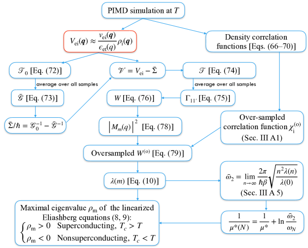
Figure 1: Flowchart of the program for analyzing PIMD outputs. $N$ denotes the cutoff of maximal $n$ when solving Eq. (8). The linear screening approximation, which should be replaced in a full implementation, is indicated by the red box.

Our program for analyzing PIMD outputs is implemented in MATLAB. Figure 1 shows the flowchart of the program. The program determines whether a PIMD simulation temperature is below or above $T_{\mathrm{c}}$. To estimate $T_{\mathrm{c}}$, one needs to run PIMD simulations at (at least) two different temperatures between which the maximal eigenvalue $\rho_{\mathrm{m}}$ of the linearized Eliashberg equations (8, 9) changes sign. $T_{\mathrm{c}}$ is estimated by a linear interpolation from the two temperatures .

In the following, we demonstrate our analyses by using the case of $P=0.7\,\mathrm{TPa}$ and $T=350\,\mathrm{K}$ as an example.

III.1.1 Density correlation function

In a PIMD, the density correlation function can be decomposed into two parts, including the self-correction function $\omega(\bm{q},\nu_{m})$ and the direct correlation function $h(\bm{q},\nu_{m})$:

$$\chi_{\mathrm{i}}(\bm{q},\nu_{m})=-\beta\rho_{0}\left[h(\bm{q},\nu_{m})+\omega(\bm{q},\nu_{m})\right],$$ (66)

where $\rho_{0}$ is the density of ions, and the definitions of the various correlation functions can be found in Ref. (Chandler and Wolynes, 1981). The self-correlation function is where the quantum effect is manifested.

To numerically evaluate the correlation functions, we first determine for each sample of the ion trajectories:

$$\tilde{\rho}_{i}(\bm{q},\nu_{m}) =\frac{1}{N_{\mathrm{b}}}\sum_{a=1}^{N_{\mathrm{b}}}e^{-i\bm{q}\cdot\bm{R}_{i}(\tau_{a})+i\nu_{m}\tau_{a}},$$ (67)

$$\rho_{\mathrm{i}}(\bm{q},\nu_{m}) =\sum_{i=1}^{N_{\mathrm{i}}}\tilde{\rho}_{i}(\bm{q},\nu_{m}).$$ (68)

The density correlation function $\chi_{\mathrm{i}}(\bm{q},\nu_{m})$ and the self-correction function $\omega(\bm{q},\nu_{m})$ can then be determined by:

$$\chi_{\mathrm{i}}(\bm{q},\nu_{m}) =-\frac{\beta\rho_{0}}{N_{\mathrm{i}}}\left\langle\left|\rho_{\mathrm{i}}(\bm{q},\nu_{m})-\left\langle\rho_{\mathrm{i}}(\bm{q},\nu_{m})\right\rangle_{\mathrm{C}}\right|^{2}\right\rangle_{\mathrm{C}},$$ (69)

$$\omega(\bm{q},\nu_{m}) =\left\langle\frac{1}{N_{\mathrm{i}}}\sum_{i=1}^{N_{\mathrm{i}}}\left|\tilde{\rho}_{i}(\bm{q},\nu_{m})\right|^{2}\right\rangle_{\mathrm{C}},$$ (70)

The direct correlation function $h(\bm{q},\nu_{m})$ can be determined by applying the identity Eq. (66).

The finite number of the beads introduces discretization errors in the determination of the correlation functions. It is the self-correlation function which is prone to the discretization errors. This can be seen in the self-correlation function of a free system (Nichols and Chandler, 1987):

$$\omega_{0}(\bm{q},\tau)=\exp\left[-\frac{1}{2}(q\lambda_{e})^{2}\frac{\tau}{\hbar\beta}\left(1-\frac{\tau}{\hbar\beta}\right)\right],$$ (71)

which becomes a sharp function of $\tau$ when $q$ is large, and cannot be accurately sampled by a small number of $N_{\mathrm{b}}$ beads.

To solve the issue, we apply an over-sampling approach. A simulation of $N_{\mathrm{b}}$ beads will give rise to a discrete set of values of $\{\omega(\bm{q},\tau_{a}),\,a=1\dots N_{\mathrm{b}}\}$. We exploit the property that $\ln\omega(\bm{q},\tau)$ is a smooth function of $\tau$, and over-sample it by interpolating from its discrete set of values. The resulting $\omega(\bm{q},\tau)$ can then be Fourier transformed to obtain an over-sampled self-correlation function $\omega^{(\mathrm{o})}(\bm{q},\nu_{m})$. By replacing $\omega(\bm{q},\nu_{m})$ with $\omega^{(\mathrm{o})}(\bm{q},\nu_{m})$ in Eq. (66), we can get an over-sampled density correlation function $\chi_{\mathrm{i}}^{(\mathrm{o})}(\bm{q},\nu_{m})$, which will be used in determining the interaction parameters (see Sec. III.1.5).

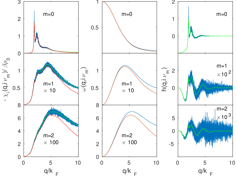
Figure 2: Various correlation functions of ions. For the density correlation function and the self correlation function, both the original one (blue) and over-sampled one (red) are shown. The data uncertainties are estimated from the fluctuation of values for the same $q$ but different $\bm{q}$’s, and indicated by vertical lines extended from/to $\pm 1$ standard deviation. The over-sampling is with an increased number of beads $N_{\mathrm{b}}^{\prime}=16N_{\mathrm{b}}$.

The correlation functions of ions are shown in Fig. 2.

III.1.2 Lippmann-Schwinger equation

We solve the Lippmann-Schwinger equation in the plane wave basis by imposing an energy cutoff of $30\,\mathrm{Ry}$. With the quasi-static approximation (see Sec. III.2), the $T$-matrix with respect to the vacuum can be obtained by:

$$\hat{\mathcal{T}}_{0}(\tau)=\left[I-\hat{V}_{\mathrm{ei}}(\tau)\hat{\mathcal{G}}_{0}\left(\omega_{N_{\mathrm{s}}}\right)\right]^{-1}\hat{V}_{\mathrm{ei}}(\tau),$$ (72)

where $[\hat{\mathcal{G}}_{0}(\omega_{N_{\mathrm{s}}})]_{\bm{k}_{1},\bm{k}_{2}}=(i\omega_{N_{\mathrm{s}}}+\mu/\hbar-\hbar k_{1}^{2}/2m_{e})^{-1}\delta_{\bm{k}_{1},\bm{k}_{2}}$, and $\hat{V}_{\mathrm{ei}}(\tau)$ is the effective ionic potential at the imaginary time $\tau$. The average Green’s function can be obtained by applying the identity:

$$\hat{\bar{\mathcal{G}}}(\omega_{N_{\mathrm{s}}})=\mathcal{\hat{G}}_{0}(\omega_{N_{\mathrm{s}}})\\ +\frac{1}{\hbar}\mathcal{\hat{G}}_{0}(\omega_{N_{\mathrm{s}}})\left\langle\frac{1}{N_{\mathrm{b}}}\sum_{a}\hat{\mathcal{T}}_{0}(\tau_{a})\right\rangle_{\mathrm{C}}\hat{\mathcal{G}}_{0}(\omega_{N_{\mathrm{s}}}).$$ (73)

The self-energy $\bar{\Sigma}(\omega_{N_{\mathrm{s}}})$ can be determined from $\bar{\mathcal{G}}(\omega_{N_{\mathrm{s}}})$, and is shown in Fig. 3. A linear fitting to the real part of the self-energy for $|k-k_{F}|<0.1k_{F}$ shows that the renormalization to the Fermi velocity is only $\sim 1.8\%$. It is ignored in our calculation of the interaction parameters.

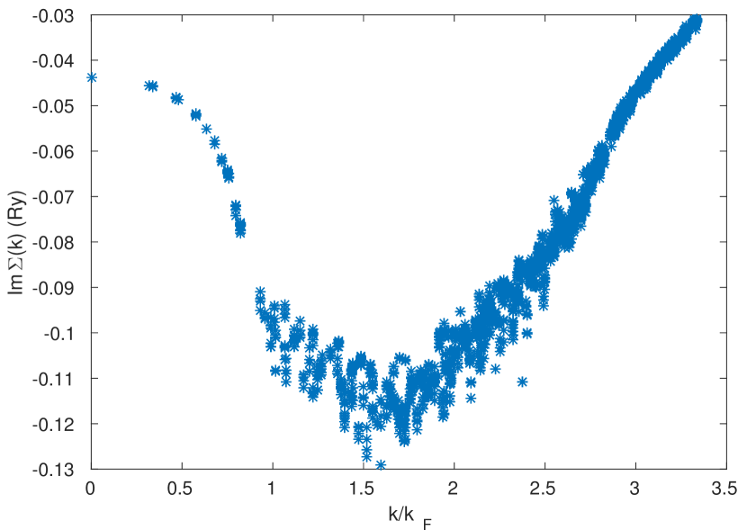
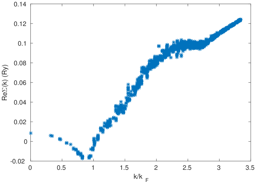
Figure 3: The imaginary and real parts of the self energy $\bar{\Sigma}$. It is evaluated in the quasi-static limit with $N_{s}=16$.

The $T$-matrix with respect to the effective medium can then be determined by:

$$\hat{\mathcal{T}}(\tau)=\left(I-\hat{\mathcal{V}}(\tau)\hat{\bar{\mathcal{G}}}\right)^{-1}\hat{\mathcal{V}}(\tau),$$ (74)

with $\hat{\mathcal{V}}(\tau)\equiv\hat{V}_{\mathrm{ei}}(\tau)-\hat{\bar{\Sigma}}$. By applying a Fourier transform [see Eq. (82)], we obtain $\mathcal{T}_{\bm{k}_{1}\bm{k}_{2}}(\nu_{m})$. The scattering amplitude is determined by:

$$\Gamma_{\bm{k}_{1}\bm{k}_{2}}(\nu_{m})=-\beta\left\langle\left|\mathcal{T}_{\bm{k}_{1}\bm{k}_{2}}(\nu_{m})\right|^{2}\right\rangle_{\mathrm{C}},$$ (75)

and is shown in Fig. 4.

III.1.3 Bethe-Salpeter equation

The effective pairing interaction can be obtained by solving the BS equation in the quasi-static limit. The effective pairing interaction at $\tau$ is determined by:

$$\hat{W}(\tau)=\left[I+\frac{1}{\hbar\beta}\hat{\Gamma}(\tau)\hat{\chi}_{0}\left(\omega_{N_{\mathrm{s}}}\right)\right]^{-1}\hat{\Gamma}(\tau),$$ (76)

where $\hat{\Gamma}(\tau)$ is the Fourier transform of $\hat{\Gamma}(\nu_{m})$, and $\hat{\chi}_{0}$ is a diagonal matrix with elements $-\hbar^{-1}|\bar{\mathcal{G}}(\omega_{N_{\mathrm{s}}},\bm{k})|^{2}$. The effective interaction $W_{\bm{k}_{1}\bm{k}_{2}}(\nu_{m})$ can then be obtained by a Fourier transform:

$$\hat{W}\left(\nu_{m}\right)=\frac{1}{\hbar\beta}\int_{0}^{\hbar\beta}\mathrm{d}\tau\hat{W}(\tau)e^{\mathrm{i}\nu_{m}\tau},$$ (77)

where $\nu_{m}\equiv 2\pi m/\hbar\beta$ is a Bosonic Matsubara frequency.

Because $|\bar{\mathcal{G}}|^{2}$ is a function sharply peaks at the Fermi surface, the equation can be solved in a truncated space span by bases with wave vectors close to the Fermi surface. In our calculation, we set a truncating condition $0.5k_{F}<|\bm{k}|<1.5k_{F}$. We numerically confirm that varying the truncating condition does not affect results.

The effective pairing interaction is shown in Fig. 4.

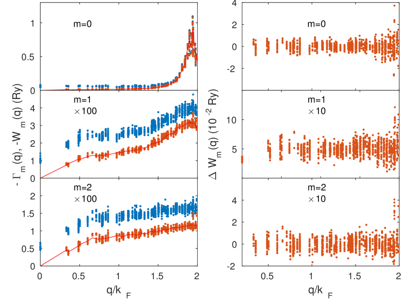
Figure 4: Scattering amplitude and the effective pairing interaction. Left: the values of $\Gamma_{\bm{k}_{1}\bm{k}_{2}}(\nu_{m})$ recast as a function of $q\equiv\left|\bm{k}_{1}-\bm{k}_{2}\right|$ for $0.9k_{F}<|\bm{k}_{1}|,|\bm{k}_{2}|<1.1k_{F}$ are shown as blue dots, and the values of $W_{\bm{k}_{1}\bm{k}_{2}}(\nu_{m})$ are shown as red dots. The red solid lines show the fitting to the model Eq. (78). Right: residues of the fitting by using $M_{m}(q)$ shown in the inset of Fig. 6.

III.1.4 Effective EPC matrix element

From Fig. 4, we observe that the effective pairing interaction vanishes at $q\rightarrow 0$ and peaks at $q\sim 2k_{\mathrm{F}}$. Similar behaviors are also observed in the density correlation function shown in Fig. 2. It suggests that the effective pairing interaction could be fitted by the relation:

$$W_{\bm{k}_{1}\bm{k}_{2}}(\nu_{m})=\left|M_{m}(q)\right|^{2}\chi_{\mathrm{i}}(\bm{k}_{1}-\bm{k}_{2},\nu_{m})$$ (78)

with $q\equiv\left|\bm{k}_{1}-\bm{k}_{2}\right|$, and $M_{m}(q)$ is interpreted as an effective EPC matrix element. We carry out the fitting by assuming $M_{m}(q)=f_{m}(q)v_{\mathrm{ei}}(q)/\epsilon_{\mathrm{et}}(q)$ with $f_{m}(q)$ being a smooth function of $q$. The smooth function is chosen to be an interpolation function of five control points at $q/2k_{F}=\{0.2,0.5,0.75,0.8725,1\}$. The values of the scaling function at these points are treated as fitting parameters. The resulting scaling functions are shown in the inset of Fig. 6. The residues of the fitting are shown in the right panel of Fig. 4. It is evident that the relation fits the numerical results remarkably well.

A good fitting to Eq. (78) is an indication of the soundness of our numerical implementation and formalism. This is because the existence of such a relation, while expected physically, is nowhere near an obvious result from our formalism. Since it takes many intermediate steps to obtain the effective pairing interaction numerically (see Fig. 1), it is unlikely that an relation like Eq. (78) could emerge from numerical results had inconsistency/inaccuracy existed in any of the intermediate steps.

III.1.5 Interaction parameters

We determine the interaction parameters $\lambda(n)$ by using Eq. (10) with the effective pairing interaction determined by:

$$W_{m}^{(\mathrm{o})}(q)=\left|M_{m}(q)\right|^{2}\chi_{\mathrm{i}}^{(\mathrm{o})}(q,\nu_{m}),$$ (79)

where $\chi_{\mathrm{i}}^{(\mathrm{o})}(q,\nu_{m})$ is the over-sampled density correlation function determined in Sec. III.1.1. The over-sampling is necessary to eliminate the discretization errors and to yield a correct asymptotic behavior of $\lambda(n)$ in the large $n$ limit. Figure 5 shows the dependence of $n^{2}\lambda(n)$ on $n$. Without the over-sampling, the values of $n^{2}\lambda(n)$ keeps increasing with $n$. With the over-sampling, $n^{2}\lambda(n)$ saturates at large $n$ as expected (Allen and Dynes, 1975). The saturation value yields an estimate of the average phonon frequency $\bar{\omega}_{2}=\lim_{n\rightarrow\infty}(2\pi/\hbar\beta)\sqrt{n^{2}\lambda(n)/\lambda}$, which enters into the Eliashberg equations by renormalizing $\mu^{\ast}$ when the equations are solved with a large-$n$ cutoff (Allen and Dynes, 1975). We take the recovery of the correct asymptotic behavior of $\lambda(n)$ as an indication of the soundness of our oversampling scheme discussed in Sec. III.1.1.

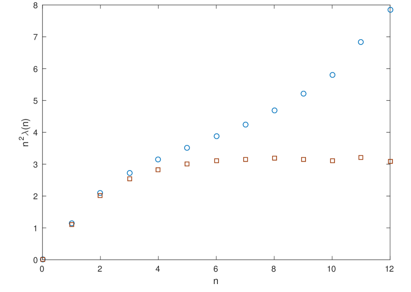
Figure 5: The values of $n^{2}\lambda(n)$ as a function of $n$. Both the values determined from the original $W_{m}(q)$ (blue circles) and the oversampled $W_{m}^{(\mathrm{o})}(q)$ (red squares) are shown.

III.2 Quasi-static approximation

An important approximation we adopt to simplify the calculation is the quasi-static approximation. Directly solving Eqs. (5–7) is numerically challenging. For instance, to solve Eq. (6) with a moderate setting of cutoffs, one may need $\sim 10^{5}$ frequency-wave-vector bases. Even worse, the solution may not have necessary accuracy because it is difficult to evaluate $\bar{\mathcal{G}}(\omega_{n})$ accurately in a PIMD simulation with a relatively small $N_{\mathrm{b}}$.

Fortunately, directly solving these time-dependent equations is not necessary. We can exploit the fact that ions move much slowly than electrons. As a result, the scattering potential $\hat{\mathcal{V}}(\tau)$ only has a few non-negligible low-frequency components. The resulting $T$-matrix will be dominated by its frequency-diagonal components $\hat{\mathcal{T}}_{nn}\equiv\hat{\mathcal{T}}(\omega_{n},\omega_{n})$, and the amplitudes of off-diagonal components $\hat{\mathcal{T}}_{mn}$ with $|\omega_{m}-\omega_{n}|\gtrsim\omega_{\mathrm{ph}}$ are negligible. For Eq. (6), we have:

$$\hat{\mathcal{T}}_{mn} =\hat{\mathcal{V}}_{m-n}+\frac{1}{\hbar}\hat{\mathcal{V}}_{m-n^{\prime}}\bar{\mathcal{G}}_{n^{\prime}}\hat{\mathcal{T}}_{n^{\prime}n}$$ (80)

$$\approx\hat{\mathcal{V}}_{m-n}+\frac{1}{\hbar}\hat{\mathcal{V}}_{m-n^{\prime}}\bar{\mathcal{G}}_{n}\hat{\mathcal{T}}_{n^{\prime}n},$$ (81)

where subscripts denote frequency components. The relative error induced by the approximation is proportional to $|\omega_{n}-\omega_{n^{\prime}}|/\omega_{n}$, and becomes negligible when $\omega_{n}\gg\left|\omega_{n}-\omega_{n^{\prime}}\right|\sim\omega_{\mathrm{ph}}$.

To solve the approximated equation, we choose $n$ to be a large integer $N_{\mathrm{s}}$ such that $\omega_{\mathrm{ph}}\ll\omega_{N_{\mathrm{s}}}\ll\epsilon_{\mathrm{F}}/\hbar$. The big disparity of the energy scales of electrons and phonons means that one can always have such a choice. The equation can be conveniently solved in the time-domain:

$$\hat{\mathcal{T}}\left(\nu_{m}+\omega_{N_{\mathrm{s}}},\omega_{N_{\mathrm{s}}}\right) =\frac{1}{\hbar\beta}\int_{0}^{\hbar\beta}\mathrm{d}\tau\hat{\mathcal{T}}_{N_{\mathrm{s}}}(\tau)e^{\mathrm{i}\nu_{m}\tau},$$ (82)

$$\hat{\mathcal{T}}_{N_{\mathrm{s}}}(\tau) =\hat{\mathcal{V}}(\tau)+\frac{1}{\hbar}\hat{\mathcal{V}}(\tau)\bar{\mathcal{G}}_{N_{\mathrm{s}}}\hat{\mathcal{T}}_{N_{\mathrm{s}}}(\tau),$$ (83)

where $\nu_{m}\equiv 2\pi m/\hbar\beta$ is a Bosonic Matsubara frequency. $\hat{\mathcal{T}}_{N_{\mathrm{s}}}(\tau)$ can be obtained for each $\tau$ by solving an elastic Lippmann-Schwinger equation by treating $\mathcal{V}(\tau)$ as if it is a static potential. We call the approximation quasi-static approximation. By inserting the solution into Eq. (5) and averaging all ionic configurations, we can obtain a scattering amplitude $\Gamma_{N_{\mathrm{s}}}(\nu_{m})\equiv\Gamma(\nu_{m}+\omega_{N_{\mathrm{s}}},\omega_{N_{\mathrm{s}}})$.

To solve the BS equation (7), we also apply the quasi-static approximation. This is to approximate the equation as

$$\hat{W}(\nu_{m}+\omega_{N_{\mathrm{s}}},\omega_{N_{\mathrm{s}}})\approx\hat{\Gamma}_{N_{\mathrm{s}}}(\nu_{m})+\frac{1}{\hbar^{2}\beta}\sum_{m^{\prime}}\\ \hat{\Gamma}_{N_{\mathrm{s}}}(\nu_{m}-\nu_{m^{\prime}})\left|\hat{\bar{\mathcal{G}}}_{N_{\mathrm{s}}}\right|^{2}\hat{W}(\nu_{m^{\prime}}+\omega_{N_{\mathrm{s}}},\omega_{N_{\mathrm{s}}}).$$ (84)

The resulting equation can then be solved in the time-domain in a similar way like Eq. (82) (See Sec. III.1.3).

It is reasonable to expect that the effective interaction $W(\nu_{m}+\omega_{n},\omega_{n})$ is close to $W(\nu_{m}+\omega_{N_{\mathrm{s}}},\omega_{N_{\mathrm{s}}})$ as long as $\hbar\left|\omega_{n}-\omega_{N_{\mathrm{s}}}\right|\ll\epsilon_{\mathrm{F}}$:

$$W(\omega_{n}+\nu_{m},\omega_{n})\approx W(\nu_{m}+\omega_{N_{\mathrm{s}}},\omega_{N_{\mathrm{s}}}).$$ (85)

It suggests that in the regime of interest with $|\omega_{n}|,|\omega_{n^{\prime}}|\ll\epsilon_{\mathrm{F}}/\hbar$, the effective interaction $\hat{W}(\omega_{n},\omega_{n^{\prime}})$ is approximately a function of $\omega_{n}-\omega_{n^{\prime}}$, and can be determined in the quasi-static limit.

We note that a similar approximation, i.e., treating $\hat{V}_{\mathrm{ei}}(\tau)$ as a static potential, is also adopted for PIMD simulations when determining atomic forces. It is customary to call the approximation as an “adiabatic approximation”. Since the particular approximation does not prevent us from determining the $\tau$-dependences of various physical quantities, it does not affect the determination of EPC in an equilibrium system. To avoid confusion, we call the approximation as a “quasi-static approximation” since it is known that EPC is intrinsically non-adiabatic and cannot be determined by an adiabatic approximation. The term “adiabatic approximation” is reserved only for the Born-Oppenheimer approximation employed by the classical molecular dynamics (see Sec. II.2.2).

III.3 Results

III.3.1 Metallic Hydrogen

We summarize the result for the case of $P=0.7\,\mathrm{TPa}$ and $T=350\,\mathrm{K}$ in Fig. 6. The effective pairing interaction matrix elements $W_{\bm{k}_{1}\bm{k}_{2}}(\omega_{N_{\mathrm{s}}}+\nu_{m},\omega_{N_{\mathrm{s}}})$ are recast as a function $W_{m}(q)$ with $q\equiv|\bm{k}_{1}-\bm{k}_{2}|$ for $\bm{k}_{1}$’s and $\bm{k}_{2}$’s close to the Fermi surface. The finiteness of the supercell of the PIMD simulation means that $W_{m}(q)$ is only defined for a discrete set of $q$-values. To this end, it is reasonable to assume that $W_{m}(q)$ is a smooth function of $q$ and can be interpolated from the discrete set of values. The effective EPC matrix element $M_{m}(q)$ is determined and shown in the inset. As opposed to the earlier theoretical effort (Jaffe and Ashcroft, 1981), the effective EPC matrix element can now be determined from first principles.

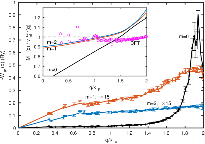
Figure 6: (Color online) Effective pairing interaction $W_{m}(q)$ with $N_{\mathrm{s}}=16$, $m=0,1,2$, and $q\equiv|\bm{k}_{1}-\bm{k}_{2}|$ with $0.9k_{F}<|\bm{k}_{1}|,|\bm{k}_{2}|<1.1k_{F}$ for a metallic hydrogen liquid at $P=700\,\mathrm{GPa}$ and $T=350\,\mathrm{K}$. The calculation is based on a PIMD simulation of $200$ hydrogen atoms and $6503$ samples of ion trajectories with the imaginary time discretized to $24$ beads (Chen et al., 2013). The scatter points and error-bars show the averages and standard deviations of $W_{m}(q)$ with same $q$ but different $\bm{k}_{1}$’s and $\bm{k}_{2}$’s. The solid lines show fittings to the model $W_{m}(q)\sim|M_{m}(q)|^{2}\chi_{\mathrm{i}}(\nu_{m},q)$. Inset: the effective EPC matrix elements $M_{m}(q)$ (solid lines), shown as ratios to the screened electron-ion potential $v_{\mathrm{ei}}^{\mathrm{scr.}}\equiv|v_{\mathrm{ei}}(q)/\epsilon_{\mathrm{et}}(q)$|. The scatter points show the ratios between the effective ionic potential determined from the DFT and that from the linear screening approximation, averaged over $1455$ ionic configurations randomly sampled from the PIMD simulation.

We carry out PIMD simulations, determine the interaction parameters and solve the Eliashberg equations for metallic hydrogen under a number of pressures and at $T=350\,\mathrm{K}$ and $450\,\mathrm{K}$. The results are summarized in Table 1. Based on the results, $T_{\mathrm{c}}$’s are estimated by linearly interpolating the values of $\rho_{\mathrm{m}}$ between the two calculated temperatures. For pressures ranging from $0.5\,\mathrm{TPa}$ to $1.5\,\mathrm{TPa}$, they are close to $400\,\mathrm{K}$, well above the melting temperatures determined in both Ref. (Chen et al., 2013) and (Geng et al., 2015).

$r_{\mathrm{s}}$		$1.226$	$1.197$	$1.17$	$1.149$	$1.113$	$1.049$
$P$		$0.5$	$0.6$	$0.7$	$0.8$	$1.0$	$1.5$
$350\mathrm{K}$	$\lambda$	$9.4(14)$	$8.5(11)$	$8.3(10)$	$6.9(9)$	$5.9(8)$	$4.8(4)$
	$\bar{\omega}_{2}$	$108(13)$	$116(13)$	$116(16)$	$129(13)$	$140(21)$	$167(26)$
	$\rho_{\mathrm{m}}$	$0.40(12)$	$0.38(11)$	$0.32(10)$	$0.30(8)$	$0.29(11)$	$0.21(9)$
$450\mathrm{K}$	$\lambda$	$7.4(13)$	$7.2(10)$	$7.2(11)$	$6.1(9)$	$5.2(7)$	$4.3(3)$
	$\bar{\omega}_{2}$	$121(27)$	$120(18)$	$121(19)$	$147(19)$	$156(20)$	$179(20)$
	$\rho_{\mathrm{m}}$	$\underline{0.06}(12)$	$\underline{0.08}(9)$	$\underline{0.31}(8)$	$\underline{0.08}(10)$	$\underline{0.12}(8)$	$\underline{0.15}(6)$
$T_{\mathrm{c}}\,(\text{K})$		$437(27)$	$433(22)$	$401(15)$	$429(25)$	$421(24)$	$408(19)$

Table 1: Mass enhancement factor $\lambda\equiv\lambda(0)$, average phonon frequency $\bar{\omega}_{2}$ (in meV), and the maximal eigenvalue $\rho_{\mathrm{m}}$ of the linearized Eliashberg equations, calculated for a number of temperatures and pressures $P$ (in $\mathrm{TPa}$). $\bar{\omega}_{2}$ is estimated by applying the asymptotic relation $\bar{\omega}_{2}=\lim_{n\rightarrow\infty}(2\pi/\hbar\beta)\sqrt{n^{2}\lambda(n)/\lambda}$ (Allen and Dynes, 1975). Negative values are indicated by underlined numbers. Numerical uncertainties are estimated by shifting the values of $W_{m}(q)$ up/down by a standard deviation simultaneously for all the discrete $q$-values, and indicated in parentheses. $T_{\mathrm{c}}$ is estimated from the linear interpolation of $\rho_{\mathrm{m}}$. We adopt $\mu^{\ast}\approx 0.089$ for the Coulomb pseudo-potential (McMahon and Ceperley, 2011). The band renormalization is found to be negligible for metallic hydrogen.

III.3.2 Metallic deuterium and isotope effect

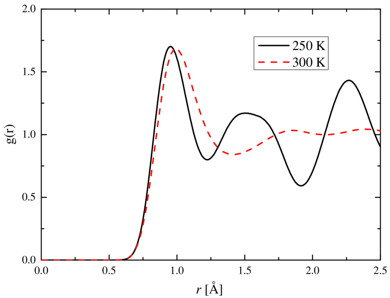
Figure 7: Radial pair distribution function $g(r)$ for deuterium at $P=1\,\mathrm{TPa}$. The functions for both $T=250\,\mathrm{K}$ (black solid line) and $T=300\,\mathrm{K}$ (red dashed line) are shown.

A test to our approach is to see whether or not it predicts the isotope effect as expected. For the purpose, we carry out PIMD simulations for metallic deuterium at $P=1\,\mathrm{TPa}$. The simulations are performed at 250, 300 and 350 K for a time interval of $5\,\mathrm{ps}$. The radial pair distribution function (RDF) $g(r)$ is calculated. As shown in Fig. 7, the RDF for $T=250\,\mathrm{K}$ shows sharp peaks, which indicates a solid state. At $T=300\,\mathrm{K}$, the sharp peaks after the first one become broad humps, which suggests a liquid state. We thus conclude that the melting temperature for deuterium at $P=1\,\mathrm{TPa}$ is between $250\,\mathrm{K}$ and $\mathrm{300\,\mathrm{K}}$.

We carry out analyses for the PIMD data. Figure 8 shows a comparison between results for hydrogen and deuterium. For the relation of $n^{2}\lambda(n)/\lambda$ vs. $n$ shown, the isotope effect predicts that the two traces would collapse into one if the deuterium data are scaled by factors $\sqrt{2}$ and 2 along the $x$- and $y$-directions, respectively. In the plot, we see that the respective factors are $\sqrt{2}$ and $2.5$. For deuterium, we determine $\hbar\bar{\omega}_{2}\approx 93\pm 9\,\mathrm{meV}$, while for hydrogen $\hbar\bar{\omega}_{2}\approx 140\pm 21\,\mathrm{meV}$ (Table 1). The ratio between the two is also close to $\sqrt{2}$ predicted by the isotope effect.

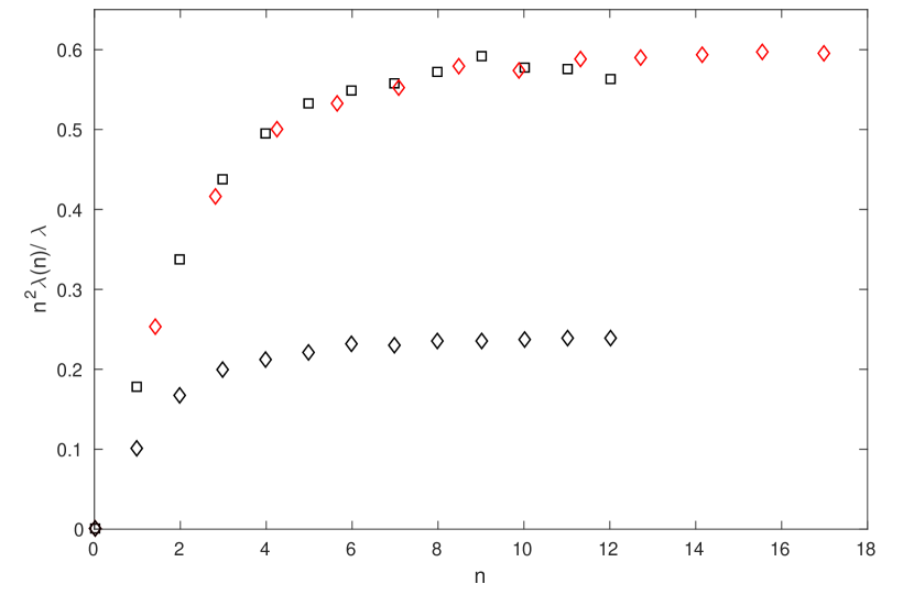
Figure 8: $n^{2}\lambda(n)/\lambda$ vs. $n$ for both metallic hydrogen (black squares) and metallic deuterium (black diamonds) at $T=350\,\mathrm{K}$ and $P=1\,\mathrm{TPa}$. For comparison, the deuterium data are also shown scaled (red diamonds) by factors $\sqrt{2}$ and 2.5 along the $x$- and $y$-directions, respectively.

To estimate $T_{\mathrm{c}}$, we analyze PIMD data at $300\,\mathrm{K}$ and $350\,\mathrm{K}$. The maximal eigenvalues of the Eliashberg equations are $-0.06\pm 0.08$ and $-0.30\pm 0.05$, respectively. It indicates that $T_{\mathrm{c}}$ is lower than $300\,\mathrm{K}$. An estimate by extrapolation yields $T_{\mathrm{c}}\approx 288\,\mathrm{K}$ for deuterium, close to the prediction of the isotope effect $421\,\mathrm{K}/\sqrt{2}\approx 298\,\mathrm{K}$.

IV Summary

In summary, we have developed a non-perturbative approach for calculating $T_{\mathrm{c}}$’s of liquids. The approach could be implemented as a first-principles tool of searching for EPC superconductivity in liquids. It predicts that a metallic hydrogen liquid is a superconducting liquid at room temperature. Experimentally, it implies that metallic hydrogen could be detected by measuring the diamagnetism induced by the Meissner effect.

Our approach can also be applied to more general systems such as (anharmonic) solids. The numerical implementation shown in this paper, however, is only applicable for metallic hydrogens for which the linear screening approximation is satisfactory. For the more general systems, it is desirable to eliminate the linear screening approximation and determine the ionic fields from first principles. This is still a work ongoing.