On the lower bound of the sum of
the algebraic connectivity of a graph and its complement

Abstract

For a graph $G$, let $\mu_{2}(G)$ denote its second smallest Laplacian eigenvalue. It was conjectured that $\mu_{2}(G)+\mu_{2}(\overline{G})\geq 1$, where $\overline{G}$ is the complement of $G$. This conjecture has been proved for various families of graphs. Here, we prove this conjecture in the general case. Also, we will show that $\max\{\mu_{2}(G),\mu_{2}(\overline{G})\}\geq 1-O(n^{-\frac{1}{3}})$, where $n$ is the number of vertices of $G$.

AMS Classification: 05C50

Keywords: Laplacian eigenvalues of graphs, Nordhaus-Gaddum type inequalities, Effective resistance, Laplacian spread

1 Introduction

Let $G$ be a simple graph with $n$ vertices. The Laplacian of $G$ is defined to be $L:=D-A$, where $A$ is the the adjacency matrix of $G$ and $D$ is the diagonal matrix of vertex degrees. The eigenvalues of $L$,

$$0=\mu_{1}(G)\leq\mu_{2}(G)\leq\cdots\leq\mu_{n}(G),$$

expose various properties of $G$. The “algebraic connectivity” of a graph $\mu(G):=\mu_{2}(G)$ is an efficient measure for connectivity of graphs.

The Laplacian spread of a graph $G$ is defined to be $\mu_{n}(G)-\mu_{2}(G)$. It was conjectured [YL12, ZSH11] that this quantity is at most $n-1$, or equivalently, $\mu_{2}(G)+\mu_{2}(\overline{G})$ is at least 1 (since $\mu_{n}(G)=n-\mu_{2}(\overline{G})$).

Conjecture.

For any graph $G$ of order $n\geq 2$, the following holds:

$$\mu(G)+\mu(\overline{G})\geq 1,$$

with equality if and only if $G$ or $\overline{G}$ is isomorphic to the join of an isolated vertex and a disconnected graph of order $n-1$.

This conjecture was proved for trees [FXWL08], unicyclic graphs [BTF09], bicyclic graphs [FLT10], tricyclic graphs [CW09], cactus graphs [Liu10], quasi-tree graphs [XM11], graphs with diameter not equal to 3 [ZSH11], bipartite graphs [ATR14], and $K_{3}$-free graphs [CD16]. Also, [AAMM18] provided a constant lower bound for $\mu(G)+\mu(\overline{G})$, by proving that $\max\{\mu(G),\mu(\overline{G})\}\geq\frac{2}{5}$.

Here, we prove the conjecture, in the general case. The main idea of the proof is as follows. Suppose that $x$ and $y$, respectively, are eigenvectors of $L(G)$ and $L(\overline{G})$, corresponding to the eigenvalues $\mu_{2}(G)$ and $\mu_{2}(\overline{G})$, with $\|x\|_{2}=\|y\|_{2}=1$. We have $\sum_{i}x_{i}=\sum_{i}y_{i}=0$ and

$$\mu(G)+\mu(\overline{G}) = {x^{T}L(G)x+y^{T}L(\overline{G})y}$$

$$= \sum_{\{i,j\}\in E(G)}(x_{i}-x_{j})^{2}+\sum_{\{i,j\}\notin E(G)}(y_{i}-y_{j})^{2}$$

$$\geq \sum_{i<j}\min\{(x_{i}-x_{j})^{2},(y_{i}-y_{j})^{2}\}.$$

So, it is enough to show that

$$\sum_{i<j}\min\{(x_{i}-x_{j})^{2},(y_{i}-y_{j})^{2}\}\geq 1.$$

Now, suppose that $M$ is the maximum of all of numbers $|x_{i}-x_{j}|^{2}$ and $|y_{i}-y_{j}|^{2}$, for every $1\leq i,j\leq n$. A simple algebraic identity (see Lemma 4), shows that $\sum_{i<j}\min\{|x_{i}-x_{j}|^{2},|y_{i}-y_{j}|^{2}\}\geq\frac{1}{M}.$ So, if $M\leq 1$, the proof is complete. It remains to consider the case $M>1$. We manage this case with some basic properties of the effective resistances between pairs of vertices of $G$ and a useful characterization of the algebraic connectivity of graphs due to Fiedler (see Lemma 2).

Moreover, here, we give an asymptotic lower bound for the maximum of $\mu(G)$ and $\mu(\overline{G})$ by proving the following theorem.

Theorem.

For all simple graphs $G$ with $n$ vertices,

$$\max\{\mu(G),\mu(\overline{G})\}\geq 1-O(n^{-\frac{1}{3}}).$$

Also, for each $n\geq 4$, there is a graph $G$ which has $n$ vertices such that the maximum of $\mu(G)$ and $\mu(\overline{G})$ is less than 1. So, if $c_{n}$ denote the minimum of $\max\{\mu(G),\mu(\overline{G})\}$ over all graphs $G$ with $n$ vertices, then $c_{n}=1-o(1)$.

The organization of the remaining of the paper is as follows. In Section 2, we gives some preliminaries and notations, which is necessary. In Section 3, we present two main results of the paper.

2 Preliminaries and notations

Throughout this paper $G$ is a simple graph, with $n\geq 2$ vertices $V(G):=\{v_{1},\ldots,v_{n}\}$ and edges $E(G)$. The notation $\{i,j\}\in E(G)$, for $i,j\in\{1,\ldots,n\}$, means that $v_{i}$ and $v_{j}$ are adjacent in $G$. Also, $A(G)$ denotes the adjacency matrix of $G$. $D(G)$ is the diagonal matrix of vertex degree. We denote the Laplacian matrix of $G$ by $L(G):=D(G)-A(G)$ and its eigenvalues by $0=\mu_{1}(G)\leq\mu_{2}(G)\leq\cdots\leq\mu_{n}(G)\leq n$ and the algebraic connectivity of $G$ by $\mu(G):=\mu_{2}(G)$. $\overline{G}$ and $\mathrm{diam}(G)$, respectively, denote the complement of $G$ and the diameter of $G$. If $v$ is a vertex of $G$, then $N_{G}(v)$ denotes the set of vertices which are adjacent to $v$ in $G$. Recall that for each $1\leq i<n$, we have $\mu_{i+1}(G)=n-\mu_{n+1-i}(\overline{G})$.

The “effective resistance” between two vertices $v_{r}$ and $v_{s}$ in a graph $G$ is denoted by $R^{G}_{r,s}$ and defined by:

$$\frac{1}{R^{G}_{r,s}}:=\min\sum_{\{i,j\}\in E(G)}(x_{i}-x_{j})^{2},$$

where the minimum runs over all $x\in\mathbb{R}^{n}$, with $x_{r}-x_{s}=1$. So for an arbitrary vector $x\in\mathbb{R}^{n}$ and $1\leq r<s\leq n$, we have

$$\sum_{\{i,j\}\in E(G)}(x_{i}-x_{j})^{2}\geq\frac{(x_{r}-x_{s})^{2}}{R^{G}_{r,s}}.$$

(In the nontrivial case $x_{r}-x_{s}\neq 0$, by dividing the vector $x$ by $x_{r}-x_{s}$, we can assume $x_{r}-x_{s}=1$ and use the defining formula for $R^{G}_{r,s}$.)

In this paper we only use some very basic properties of the effective resistance which are listed in the following lemma:

Lemma 1.

Let $G=(V,E)$ be a simple graph with $n\geq 2$ vertices. Then the following holds:

• For every subgraph $H$ of $G$ which contains the vertices $v_{1}$ and $v_{2}$, $R^{G}_{1,2}\leq R^{H}_{1,2}$.

• “Total resistance of parallel circuits”: Let $G_{1}$ and $G_{2}$ be two subgraphs of $G$, such that $V(G_{1})\cap V(G_{2})=\{v_{1},v_{2}\}$ and $E(G)$ be the disjoint union of $E(G_{1})$ and $E(G_{2})$. Then

  $$\frac{1}{R^{G}_{1,2}}=\frac{1}{R^{G_{1}}_{1,2}}+\frac{1}{R^{G_{2}}_{1,2}}.$$

• “Total resistance of series circuits”: For $n\geq 3$, let $G_{1}$ and $G_{2}$ be two induced subgraphs of $G$, such that $v_{1}\in V(G_{1})$, $v_{3}\in V(G_{2})$ and $V(G_{1})\cap V(G_{2})=\{v_{2}\}$. Suppose also that $E(G)$ be the disjoint union of $E(G_{1})$ and $E(G_{2})$. Then

  $$R^{G}_{1,3}=R^{G_{1}}_{1,2}+R^{G_{2}}_{2,3}$$

Proof.

The parts (a) and (b) are immediate from the defining equation of the effective resistance. For (c), we have:

$$\frac{1}{R^{G}_{1,3}} = \min_{x\in\mathbb{R}^{n},x_{1}=0,x_{3}=1}\sum_{\{i,j\}\in E(G)}(x_{i}-x_{j})^{2}$$

$$= \min_{x\in\mathbb{R}^{n},x_{1}=0,x_{3}=1}\sum_{\{i,j\}\in E(G_{1})}(x_{i}-x_{j})^{2}+\sum_{\{i,j\}\in E(G_{2})}(x_{i}-x_{j})^{2}$$

$$= \min_{x_{2}\in\mathbb{R},x_{1}=0,x_{3}=1}\frac{(x_{1}-x_{2})^{2}}{R^{G_{1}}_{1,2}}+\frac{(x_{2}-x_{3})^{2}}{R^{G_{2}}_{2,3}}$$

$$= \min_{x_{2}\in\mathbb{R}}\frac{x_{2}^{2}}{R^{G_{1}}_{1,2}}+\frac{(x_{2}-1)^{2}}{R^{G_{2}}_{2,3}}$$

$$= \frac{1}{R^{G_{1}}_{1,2}+R^{G_{2}}_{2,3}}.$$

(The equality of the second and the third line, uses the fact that $G_{1}$ and $G_{2}$ have only the vertex $v_{2}$ in common.) ∎

We conclude this section with a useful lemma, due to Fiedler.

Lemma 2 ([Fie75]).

Let $G=(V,E)$ be a connected graph. Then $\mu(G)$ is positive and equal to the minimum of the function

$$\varphi(x):=n\frac{\sum_{\{i,j\}\in E(G)}(x_{i}-x_{j})^{2}}{\sum_{i<j}(x_{i}-x_{j})^{2}}$$

over all nonconstant $n$-tuples $x=(x_{1},\ldots,x_{n})\in\mathbb{R}^{n}$ (i.e. $n$-tuples which are not of the form $x_{i}=c,i=1,\ldots,n$).

Therefore $\mu(G)$ is the largest real number for which the following inequality holds for every $x=(x_{1},\ldots,x_{n})\in\mathbb{R}^{n}$:

$$n\sum_{\{i,j\}\in E(G)}(x_{i}-x_{j})^{2}\geq\mu(G)\sum_{i<j}(x_{i}-x_{j})^{2}.$$ (1)

3 Main results

3.1 Sum of the algebraic connectivity of a graph and its complement

Theorem 1.

For any graph $G$ of order $n\geq 2$, the following holds:

$$\mu(G)+\mu(\overline{G})\geq 1,$$

with equality if and only if $G$ or $\overline{G}$ is isomorphic to the join of an isolated vertex and a disconnected graph of order $n-1$.

Note that for any connected graph $G$, $\mu(G)$ is a positive number. So, when $G$ is a disconnected graph, Theorem 1 can be reformulated as the following lemma:

Lemma 3.

If $G$ is a disconnected graph, then $\mu(\overline{G})\geq 1$, with equality if and only if $\overline{G}$ is the join of an isolated vertex and a disconnected graph.

Proof.

We know that the biggest Laplacian eigenvalue of every graph is at most the number of its vertices and the Laplacian eigenvalues of $G$ are the union of the eigenvalues of its connected components, where each of which has less than $n$ vertices. So, $\mu_{n}(G)\leq n-1$ and $\mu(\overline{G})=n-\mu_{n}(G)\geq 1$, with equality if and only if $G$ is the disjoint union of an isolated vertex and a connected graph $H$ with $n-1$ vertices, where $\mu_{n-1}(H)=n-1$. But, note that $\mu_{n-1}(H)=n-1-\mu_{2}(\overline{H})$. So, we have $\mu_{n-1}(H)=n-1$, if and only if $\overline{H}$ is disconnected. Therefore, we have equality $\mu(\overline{G})=1$, if and only if $\overline{G}$ is the join of an isolated vertex and a disconnected graph $\overline{H}$. ∎

Lemma 4.

Let $x=(x_{1},\ldots,x_{n})$ and $y=(y_{1},\ldots,y_{n})$ be two vectors in $\mathbb{R}^{n}$ with $\sum_{i}y_{i}=\sum_{i}x_{i}=0$. Then

$$\sum_{i<j}(x_{i}-x_{j})^{2}(y_{i}-y_{j})^{2}\geq\|x\|^{2}\|y\|^{2}.$$

Proof.

Denote $A=\sum_{i<j}(x_{i}-x_{j})^{2}(y_{i}-y_{j})^{2}$. We have

$$2A = \sum_{i\neq j}(x_{i}-x_{j})^{2}(y_{i}-y_{j})^{2}$$

$$= \sum_{i,j}(x_{i}-x_{j})^{2}(y_{i}-y_{j})^{2}\quad\mbox{(The terms corresponding to values $i=j$ are zero)}$$

$$= \sum_{i,j}(x_{i}^{2}+x_{j}^{2}-2x_{i}x_{j})(y_{i}^{2}+y_{j}^{2}-2y_{i}y_{j})$$

$$= \sum_{i,j}(x_{i}^{2}y_{i}^{2}+x_{j}^{2}y_{j}^{2})+\sum_{i,j}(x_{i}^{2}y_{j}^{2}+x_{j}^{2}y_{i}^{2})+4\sum_{i,j}x_{i}x_{j}y_{i}y_{j}$$

$$-2\sum_{i,j}\big{(}x_{i}^{2}y_{i}y_{j}+x_{j}^{2}y_{i}y_{j}+x_{i}x_{j}y_{i}^{2}+x_{i}x_{j}y_{j}^{2}\big{)}$$

$$= 2\sum_{i,j}x_{i}^{2}y_{i}^{2}+2\sum_{i,j}x_{i}^{2}y_{j}^{2}+4\sum_{i,j}x_{i}x_{j}y_{i}y_{j}-4\sum_{i,j}\Big{(}x_{i}^{2}y_{i}y_{j}+x_{i}x_{j}y_{i}^{2}\Big{)}$$

$$= 2n\sum_{i}x_{i}^{2}y_{i}^{2}+2\Big{(}\sum_{i}x_{i}^{2}\Big{)}\Big{(}\sum_{j}y_{j}^{2}\Big{)}+4\Big{(}\sum_{i}x_{i}y_{i}\Big{)}\Big{(}\sum_{j}x_{j}y_{j}\Big{)}$$

$$-4\Big{(}\sum_{i}x_{i}^{2}y_{i}\Big{)}\Big{(}\sum_{j}y_{j}\Big{)}-4\Big{(}\sum_{i}x_{i}y_{i}^{2}\Big{)}\Big{(}\sum_{j}x_{j}\Big{)}$$

$$= 2n\sum_{i}x_{i}^{2}y_{i}^{2}+2\Big{(}\sum_{i}x_{i}^{2}\Big{)}\Big{(}\sum_{i}y_{i}^{2}\Big{)}+4\Big{(}\sum_{i}x_{i}y_{i}\Big{)}^{2}\quad{(\mbox{by $\sum_{j}x_{j}=\sum_{j}y_{j}=0$})}$$

$$\geq 2\|x\|^{2}\|y\|^{2}.$$

∎

Lemma 5.

Suppose that $G$ is a connected graph with $n\geq 2$ vertices $\{v_{1},\ldots,v_{n}\}$. Let $x=(x_{1},\ldots,x_{n})$ be an eigenvector of $L(G)$ corresponding to $\mu_{2}(G)$. If

$$x_{1}=\max_{i}x_{i},\quad x_{2}=\min_{i}x_{i},$$

and the distance between $v_{1}$ and $v_{2}$ is at most equal to $2$, then $\mu(G)\geq 1$. In particular, for any graph with diameter less than $3$, we have $\mu(G)\geq 1$.

Proof.

Since $x$ is orthogonal to the constant-entries vector $(1,\ldots,1)$, $\sum_{i}x_{i}=0$. So, $x_{2}<0<x_{1}$. Now, from $L(G)x=\mu x$, we get $\mu x_{1}=\sum_{\{i,1\}\in E(G)}(x_{1}-x_{i})$. But, for each $i$, $x_{1}-x_{i}\geq 0$. Thus, for every $v_{i}\sim v_{1}$, we have $x_{1}-x_{i}\leq\mu x_{1}$, or equivalently, $x_{i}\geq(1-\mu)x_{1}$. Similarly, for every $v_{j}\sim v_{2}$, we have $x_{j}\leq(1-\mu)x_{2}$. Therefore, if $\mu<1$, for every $v_{i}\sim v_{1}$ and $v_{j}\sim v_{2}$ we have $x_{j}<0<x_{i}$. So $v_{1}$ and $v_{2}$ are not adjacent and have no common neighbor. Thus, the distance between $v_{1}$ and $v_{2}$ is greater than $2$. ∎

Proof of Theorem 1.

According to Lemma 3, we can suppose that both $G$ and $\overline{G}$ are connected. So, we have $n>2$. Denote $\mu_{2}(G)$ and $\mu_{2}(\overline{G})$, respectively by $\mu$ and $\overline{\mu}$. Let $x=(x_{1},\ldots,x_{n})$ be a normalized eigenvector of $L(G)$ corresponding to $\mu_{2}(G)$ and $y=(y_{1},\ldots,y_{n})$ be a normalized eigenvector of $L(\overline{G})$ corresponding to $\mu_{2}(\overline{G})$. Note that $y$ is also an eigenvector of $L(G)$ corresponding to $\mu_{n}(G)$. So $x$ and $y$ are two orthonormal vectors in $\mathbb{R}^{n}$ which are orthogonal to $e=(1,\ldots,1)$ (the eigenvector of $\mu_{1}(G)=0$). Now, without loss of generality, we can suppose that $\max_{i<j}|x_{i}-x_{j}|\geq\max_{i<j}|y_{i}-y_{j}|$ and

$$x_{1}=\max_{1\leq i\leq n}x_{i},\quad x_{2}=\min_{1\leq i\leq n}x_{i}.$$

Note that since $\sum_{i}x_{i}=0$ and $x$ is nonzero, we have $x_{2}<0<x_{1}$.

Step 1 (the case $x_{1}-x_{2}<1$).

We have

$$\mu+\overline{\mu} = \sum_{\{i,j\}\in E(G)}(x_{i}-x_{j})^{2}+\sum_{\{i,j\}\in E(\overline{G})}(y_{i}-y_{j})^{2}$$

$$\geq \sum_{i<j}\min\{(x_{i}-x_{j})^{2},(y_{i}-y_{j})^{2}\}$$

$$\geq \frac{\sum_{i<j}(x_{i}-x_{j})^{2}(y_{i}-y_{j})^{2}}{\max_{i<j}\max\{(x_{i}-x_{j})^{2},(y_{i}-y_{j})^{2}\}}$$

$$\geq \frac{\|x\|^{2}\|y\|^{2}}{(x_{1}-x_{2})^{2}}\qquad\mbox{(by Lemma \ref{lem:identity})}$$

$$= \frac{1}{(x_{1}-x_{2})^{2}}.\qquad\mbox{{(since $x$ and $y$ are normalized)}}$$

The first inequality is implied by the fact that, for every pair $i<j$, $\{i,j\}$ is an edge for exactly one of $G$ or $\overline{G}$. For the second inequality, note that:

$$(x_{i}-x_{j})^{2}(y_{i}-y_{j})^{2}\!\!\!\!\! = \!\!\!\min\{(x_{i}-x_{j})^{2},(y_{i}-y_{j})^{2}\}\max\{(x_{i}-x_{j})^{2},(y_{i}-y_{j})^{2}\}$$

$$\leq \!\!\!\!\min\{(x_{i}-x_{j})^{2},(y_{i}-y_{j})^{2}\}{\max_{k<l}\max\{(x_{k}-x_{l})^{2},(y_{k}-y_{l})^{2}\}}.$$

Thus, in the case $x_{1}-x_{2}<1$, we have $\mu+\overline{\mu}>1$ and the proof is complete. So, we can suppose that $x_{1}-x_{2}\geq 1$.

Step 2 (the case $x_{1}-x_{2}\geq 1$).

Since $\mu$ and $\overline{\mu}$ are positive, if one of them is greater than or equal to $1$ then $\mu+\overline{\mu}>1$. So, we can suppose that $\mu,\overline{\mu}<1$. Let $d$ be the distance between $v_{1}$ and $v_{2}$ in $G$.

Step 2.1 ($d\leq 2$ or $d>3$).

If $d\leq 2$ then, by Lemma 5, we have $\mu\geq 1$. On the other hand, if $d>3$ then $\mathrm{diam}(G)>3$. So the diameter of $\overline{G}$ is at most equal to $2$. Thus, by Lemma 5, $\overline{\mu}\geq 1$. Therefore, we can suppose that $d=3$.

Step 2.2 ($d=3$).

Now, suppose that $s\geq 1$ is the maximum number of vertex-disjoint paths with length 3 between two vertices $v_{1},v_{2}$ in $G$.

Let $S$ be the union of the vertices of $s$ disjoint paths between $v_{1}$ and $v_{2}$ with length $3$. Denote $S_{1}:=S\cap N_{G}(v_{2})$ and $S_{2}:=S\cap N_{G}(v_{1})$ (see Figure 1). Note that because $v_{1}$ and $v_{2}$ have no common neighbor in $G$, the vertices of $S_{1}$ are not adjacent to $v_{1}$ and the vertices of $S_{2}$ are not adjacent to $v_{2}$. Also, $|S_{1}|=|S_{2}|=s$ and $S=S_{1}\cup S_{2}\cup\{v_{1},v_{2}\}$. Therefore, if we denote $A:=N_{G}(v_{1})\setminus S$, $B:=N_{G}(v_{2})\setminus S,$ and $C:=V(G)\setminus(A\cup B\cup S)$ then $\{A,B,C,S_{1},S_{2},\{v_{1},v_{2}\}\}$ is a partition of the vertices of $G$ and because by the maximality of $s$, there is no path of length at most 3 between $v_{1}$ and $v_{2}$ in $G\setminus(S_{1}\cup S_{2})$, no vertex of $A\cup\{v_{1}\}$ is adjacent to any of the vertices of $B\cup\{v_{2}\}$.

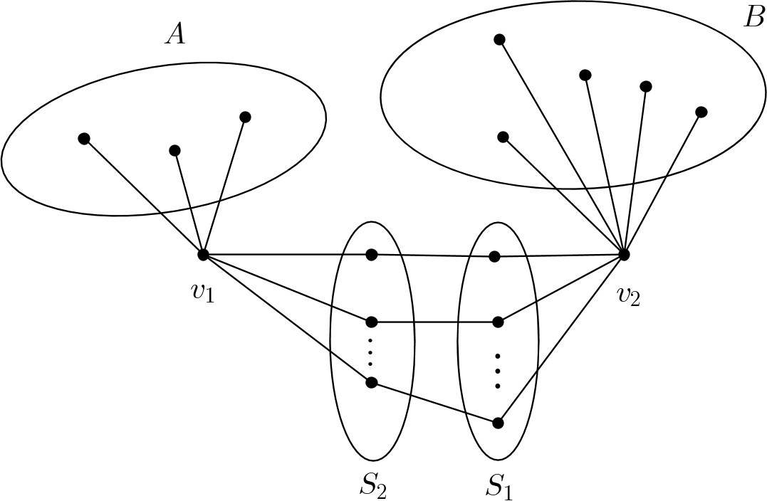
Figure 1: The subsets $S_{1},S_{2},A$ and $B$ of the vertices of $G$.

Now, if we let $a:=|A|,b:=|B|$ and $c:=|C|$, then

$$n=a+b+c+2s+2.$$ (2)

Furthermore we can suppose that $a\leq b$.

Suppose that $l$ is the maximum of $|N_{G}(v)\cap A|$ for all $v\in S_{1}$ and $|N_{G}(u)\cap B|$ for all $u\in S_{2}$. So $G$ contains a subgraph $G_{1}$, as illustrated in Figure 2. We have

$$\mu\geq\frac{(x_{1}-x_{2})^{2}}{R^{G}_{1,2}}\geq\frac{1}{R^{G}_{1,2}}.$$

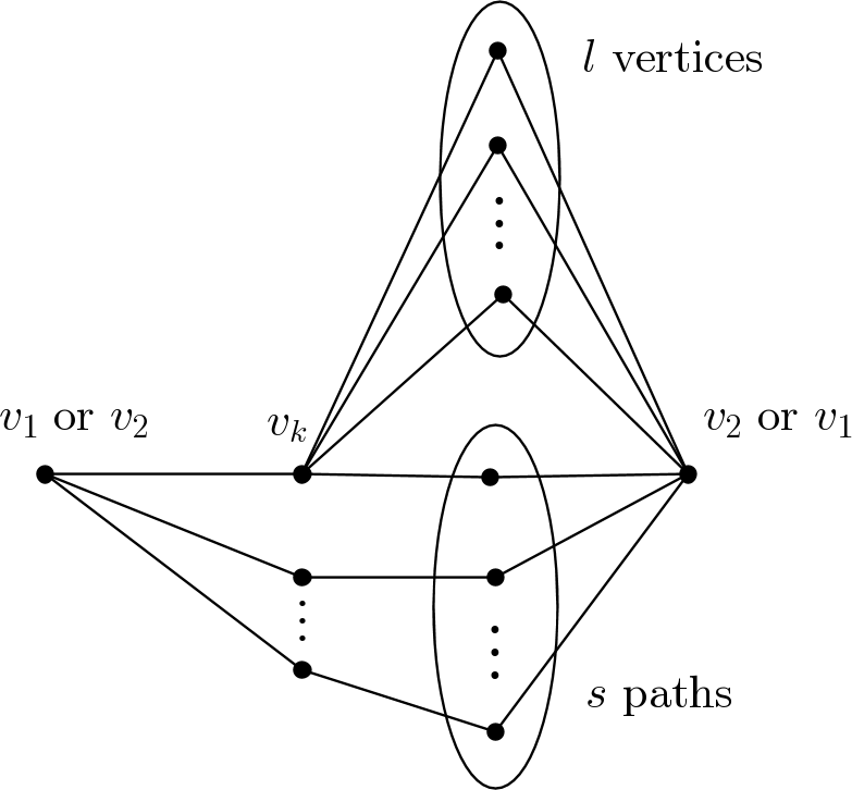
Figure 2: $G_{1}$: A subgraph of $G$.

By part (a) of Lemma 1, $R^{G}_{1,2}\leq R^{G_{1}}_{1,2}$. By multiple usage of the rules of total resistance for parallel and series circuits in Lemma 1, we have:

$$\frac{1}{R^{G_{1}}_{1,2}}=\frac{1}{1+\frac{1}{\underbrace{\frac{1}{2}+\cdots+\frac{1}{2}}_{l+1\text{ times}}}}+\underbrace{\frac{1}{3}+\cdots+\frac{1}{3}}_{s-1\text{ times}}+=\frac{1}{1+\frac{2}{l+1}}+\frac{s-1}{3}=\frac{l+1}{l+3}+\frac{s-1}{3}.$$

(The terms $\frac{1}{2}$ correspond to $l+1$ parallel paths of length $2$ between $v_{k}$ and $v_{2}$ or $v_{1}$ in $G_{1}$. Also the terms $\frac{1}{3}$ correspond to $s-1$ parallel paths of length $3$ not including $v_{k}$ between $v_{1}$ and $v_{2}$ in $G_{1}$, as in the Figure 2).

Finally we have a lower bound for $\mu$ in terms of $s$ and $l$:

$$\mu\geq\frac{s-1}{3}+\frac{l+1}{l+3}.$$ (3)

Next, we give a lower bound for $\overline{\mu}$. Note that $\overline{G}$ contains the edges of the graph illustrated in Figure 3, which hereafter is called $G_{2}$. Also, according to the definition of $l$, each vertex of $S_{1}$ are adjacent to at most $l$ vertices of $A$ in $G$ and each vertex of $S_{2}$ are adjacent to at most $l$ vertices of $B$ in $G$.

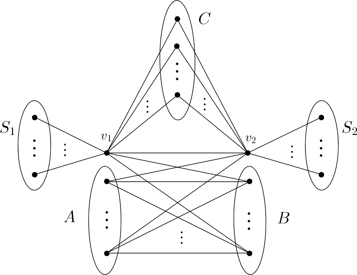
Figure 3: $G_{2}$: A subgraph of $\overline{G}$.

Now, we define the subgraphs $H_{1},H_{2}$ and $H_{3}$ of $\overline{G}$ as follows: (see figure 4)

Figure 4: Graphs $H_{1},H_{2}$ and $H_{3}$.

1. $H_{1}$ is the union of the edges which join $v_{1}$ to the vertices of $\{v_{2}\}\cup B\cup C\cup S_{1}$,

2. $H_{2}$ is the union of the edges which join $v_{2}$ to the vertices of $A\cup C\cup S_{2}$,

3. $H_{3}$ is the union of the edges which join $v_{2}$ to the vertices of $\{v_{1}\}\cup A\cup S_{2}$.

Next, note that each of $H_{1},H_{2},$ and $H_{3}$ is a star graph. Thus, $\mu(H_{i})=1,$ for $i=1,2,3.$ So, if we define

$$X = \{(i,j):(v_{i},v_{j})\in\mathrm{V}(H_{1})^{2}\cup\mathrm{V}(H_{2})^{2}\cup\mathrm{V}(H_{3})^{2}\}$$

$$= \{(i,j):(v_{i},v_{j}),(v_{j},v_{i})\not\in(S_{1}\times S_{2})\cup(S_{1}\times A)\cup(S_{2}\times B)\cup(A\times B)\},$$

by inequality (1), one can easily verify that

$$\begin{split}\sum_{\begin{subarray}{c}(i,j)\in X\\ i<j\end{subarray}}(y_{i}-y_{j})^{2}\quad\leq\quad&(b+c+s+2)\sum_{\{i,j\}\in E(H_{1})}(y_{i}-y_{j})^{2}\ \\ &+(a+c+s+1)\sum_{\{i,j\}\in E(H_{2})}(y_{i}-y_{j})^{2}\ \\ &+(a+s+2)\sum_{\{i,j\}\in E(H_{3})}(y_{i}-y_{j})^{2}\ .\end{split}$$ (4)

Since the resistance of a path with length $3$ is equal to $3$, we have

$$\sum_{\begin{subarray}{c}v_{i}\in S_{1}\\ v_{j}\in S_{2}\end{subarray}}(y_{i}-y_{j})^{2} \leq 3\sum_{\begin{subarray}{c}v_{i}\in S_{1}\\ v_{j}\in S_{2}\end{subarray}}\big{(}(y_{i}-y_{1})^{2}+(y_{1}-y_{2})^{2}+(y_{2}-y_{j})^{2}\big{)}$$

$$=3s\sum_{v_{i}\in S_{1}}(y_{1}-y_{i})^{2}+3s\sum_{v_{j}\in S_{2}}(y_{2}-y_{j})^{2}+3s^{2}(y_{1}-y_{2})^{2}.$$ (5)

Also, if we define $A_{i}:=A\setminus N_{\overline{G}}(v_{i})$, for each $v_{i}\in S_{1}$, then $|A_{i}|\leq l$, for each $v_{i}\in S_{i}$, and

$$\begin{split}\sum_{v_{i}\in S_{1}}\sum_{v_{j}\in A_{i}}(y_{i}-y_{j})^{2}\ &\leq 3\sum_{v_{i}\in S_{1}}\sum_{v_{j}\in A_{i}}\big{(}(y_{i}-y_{1})^{2}+(y_{1}-y_{2})^{2}+(y_{2}-y_{j})^{2}\big{)}\\ &\leq 3sl\Big{(}\sum_{v_{i}\in S_{1}}(y_{i}-y_{1})^{2}+\sum_{v_{j}\in A}(y_{2}-y_{j})^{2}+(y_{1}-y_{2})^{2}\Big{)}.\end{split}$$ (6)

Similarly, if we define $B_{i}:=B\setminus N_{\overline{G}}(v_{i})$, for each $v_{i}\in S_{2}$, we have

$$\sum_{\begin{subarray}{c}v_{i}\in S_{2}\\ v_{j}\in B_{i}\end{subarray}}(y_{i}-y_{j})^{2}\leq 3sl\Big{(}\sum_{v_{i}\in S_{2}}(y_{i}-y_{2})^{2}+\sum_{v_{j}\in B}(y_{1}-y_{j})^{2}+(y_{1}-y_{2})^{2}\Big{)}.$$ (7)

On the other hand, for all pairs $(i,j)$ such that $v_{i}\in S_{1}$ and $v_{j}\in A\setminus A_{i}$, or $v_{i}\in S_{2}$ and $v_{j}\in B\setminus B_{i}$, or $v_{i}\in A$ and $v_{j}\in B$, we have the trivial inequality

$$(y_{i}-y_{j})^{2}\leq(y_{i}-y_{j})^{2}.$$ (8)

Now, note that for all of the terms $(y_{i}-y_{j})^{2}$ which appear in the right hand side of the inequalities (4),(3.1),(6),(7), and (8), we have $\{i,j\}\in E(\overline{G})$, and on the other hand, for each $i<j$, one of $(y_{i}-y_{j})^{2}$ or $(y_{j}-y_{i})^{2}$ appears in the left hand side of one of these inequalities. Since $H_{1}$ and $H_{2}$ have no common edges, $b+c+s+2\geq a+c+s+1$, and the terms $(y_{i}-y_{j})^{2}$ which appear in (8) does not appear in other inequalities, by summing up both sides of these inequalities, we will get

$$\sum_{i<j}(y_{i}-y_{j})^{2} \leq \Big{(}(b+c+s+2)+(a+s+2)+3s^{2}+3sl+3sl\Big{)}$$ (9)

$$\times\sum_{\{i,j\}\in E(\overline{G})}(y_{i}-y_{j})^{2}$$

$$= (n+2+3s^{2}+6sl)\sum_{\{i,j\}\in E(\overline{G})}(y_{i}-y_{j})^{2}.\qquad{\mbox{(by \eqref{n})}}$$

But $y=(y_{1},\dots,y_{n})$ is an eigenvector of $L(\overline{G})$ corresponding to $\overline{\mu}$ with $\sum_{i}y_{i}=0$, so have

$$\sum_{\{i,j\}\in E(\overline{G})}(y_{i}-y_{j})^{2}=y^{T}L(\overline{G})\,y=\overline{\mu}\|y\|^{2}=\frac{\overline{\mu}}{n}\sum_{i<j}(y_{i}-y_{j})^{2}.$$

Therefore

$$\overline{\mu}\geq\frac{n}{n+2+3s^{2}+6sl}.$$ (10)

A lower bound for $\mu+\overline{\mu}$.

Therefore, by inequalities (3) and (10),

$$\mu+\overline{\mu}\geq\frac{n}{n+2+3s^{2}+6sl}+\frac{s-1}{3}+\frac{l+1}{l+3}.$$ (11)

Now by inequality (3), for $s\geq 3$, we have $\mu\geq 1$. So we can suppose that $s=1\,\text{or}\,2$.

The case $s=1$.

In this case,

$$\mu+\overline{\mu}\geq\frac{l+1}{l+3}+\frac{n}{n+5+6l}.$$

Thus, for each $n\geq 12$,

$$\mu+\overline{\mu}\geq 1-\frac{2}{l+3}+\frac{12}{17+6l}>1.$$

The case $s=2$.

Similarly, in this case,

$$\mu+\overline{\mu}\geq\frac{1}{3}+\frac{l+1}{l+3}+\frac{n}{n+14+12l}.$$

Note that, when $l\geq 3$, $\mu\geq\frac{1}{3}+\frac{l+1}{l+3}\geq 1$. So, $\mu+\overline{\mu}>1$. Also, for each of cases $l=0,1,2$, when $n\geq 10$,

$$l=0: \qquad\mu+\overline{\mu}\geq\frac{2}{3}+\frac{10}{24}>1,$$

$$l=1: \qquad\mu+\overline{\mu}\geq\frac{1}{3}+\frac{1}{2}+\frac{10}{36}>1,$$

$$l=2: \qquad\mu+\overline{\mu}\geq\frac{1}{3}+\frac{3}{5}+\frac{10}{48}>1.$$

For all of the remaining cases, the theorem can be checked numerically as follows:

• $n\leq 4$. The only connected graph $G$ with connected complement, is $P_{4}$ the path graph of length $3$. In this case:

  $$\mu+\overline{\mu}=2\mu(P_{4})=2(2-\sqrt{2})>1.$$

• $s=2,n\leq 9$. $G_{2}$ is a subgraph of $\overline{G}$ and so $\mu(G_{2})\leq\overline{\mu}$. The graph $G_{2}$ only depends on the nonnegative integers $a,b,c$ with constraints $s=2$ and $a+b+c+2s+2=n\leq 9$ (at most $n^{3}$ cases for each $n$). The minimum of the values of $\mu(G_{2})$ in all of these cases is approximately $0.357$, and so by (3) we have

  $$\mu+\overline{\mu}>\frac{2}{3}+0.35>1.$$

• $s=1,\;5\leq n\leq 11$. In these cases also the values of the second Laplacian eigenvalues of all graphs $G_{2}$ can be computed numerically and the minimum is approximately $0.429$. So again by (3), for $l\geq 2$ we have

  $$\mu+\overline{\mu}>\frac{l+1}{l+3}+0.42>1.$$

  For the remaining cases $l=0,1$, $|S_{1}|=|S_{2}|=s=1$ and note that by the definition of $l$, the vertex in $S_{1}=\{u\}$ is adjacent in $G$ to at most $l$ vertices in $A$, and also the vertex in $S_{2}=\{v\}$ is adjacent in $G$ to at most $l$ vertices in $B$. Let $G_{3}$ be the graph obtained from $G_{2}$ by adding the edges in $\overline{G}$ between $u$ and $A$ and also edges between $v$ and $B$.

  In the case $l=0$, $G_{3}$ is only dependent (up to isomorphism) on the size of the sets $A,B,C$ (at most $n^{3}$ cases for each $n$), and by computation for $5\leq n\leq 11$ the minimum of $\mu(G_{3})$ is approximately $0.697$. Now $G_{3}$ is a subgraph of $\overline{G}$ and again by (3),

  $$\mu+\overline{\mu}\geq\frac{1}{3}+\mu(G_{3})>\frac{1}{3}+0.69>1.$$

  In the case $l=1$, $u$ is adjacent in $G_{3}$ to all vertices in $A$ except at most one vertex and also the same happens for $v$ and $B$. By deletion of edges (if necessary) we can suppose that $A=\emptyset$ or $u$ is nonadjacent in $G_{3}$ to exactly one vertex in $A$, and also the simillar thing for $v$ with respect to $B$. Again the graph $G_{3}$ depends only (up to isomorphism) on the size of the sets $A,B,C$ and for $n\leq 11$ the minimum of $\mu(G_{3})$ is approximately $0.518$. So we have

  $$\mu+\overline{\mu}\geq\frac{l+1}{l+3}+\mu(G_{3})>\frac{1}{2}+0.51>1.$$

Thus, the theorem holds for every $n\geq 2$. ∎

3.2 Maximum of the algebraic connectivity of a graph and its compelement

As a by-product of the proof of Theorem 1, we prove the following theorem.

Theorem 2.

For all graphs $G$ with $n$ vertices,

$$\max\{\mu(G),\mu(\overline{G})\}\geq 1-O(n^{-\frac{1}{3}}).$$

Proof.

It is sufficient to prove the theorem for a connected graph $G$ with $n$ vertices, for sufficiently large integers $n$. With the notations and assumptions at the beginning of the proof of Theorem 1, we know

$$\mu+\overline{\mu}\geq\frac{1}{(x_{1}-x_{2})^{2}}.$$

So, if $(x_{1}-x_{2})^{2}\leq\frac{1}{2}$, then $\mu+\overline{\mu}\geq 2$ and the maximum of $\mu$ and $\overline{\mu}$ is at least $1$. Thus we can suppose that $(x_{1}-x_{2})^{2}\geq\frac{1}{2}$. Now, similar to Step 2 of the proof of Theorem 1, we can suppose that both $\mu$ and $\overline{\mu}$ are smaller than $1$. This implies that the distance between $v_{1}$ and $v_{2}$ in $G$ is equal to $3$. Let $s\geq 1$ be the maximum number of vertex-disjoint paths with length 3 between two vertices $v_{1}$ and $v_{2}$ in $G$. Therefore,

$$1>\mu\geq\frac{(x_{1}-x_{2})^{2}}{R^{G}_{1,2}}\geq\frac{1}{2}\times\frac{s}{3}=\frac{s}{6}.$$

So $s\leq 5$. Now, by (10), with the notations which was defined in Step 2.2 of the proof of Theorem 1, we have

$$\overline{\mu}\geq\frac{n}{n+2+3s^{2}+6sl}\geq\frac{n}{n+80+30l}.$$

On the other hand, note that according to the definition of $l$, $G$ contains the subgraph $G_{1}$ which is illustrated in Figure 2. Without loss of generality, we can assume that the left vertex in Figure 2 is $v_{1}$ and the right vertex is $v_{2}$. Now we have

$$\mu x_{1}=\sum_{\{1,i\}\in E(G)}(x_{1}-x_{i})\geq(x_{1}-x_{k}).$$

So $x_{k}\geq(1-\mu)x_{1}$ and $x_{k}-x_{2}\geq(1-\mu)(x_{1}-x_{2})$. Therefore,

$$1>\mu=\sum_{\{i,j\}\in E(G)}(x_{i}-x_{j})^{2}\geq\frac{(x_{k}-x_{2})^{2}}{R_{k,2}^{G}}\geq(1-\mu)^{2}\times\frac{1}{2}\times\frac{l+1}{2}.$$

Thus, $(1-\mu)^{2}\leq\frac{4}{l+1}$ and $\mu\geq 1-\frac{2}{\sqrt{l+1}}$. Now, we consider two cases:

1. $n<l^{\frac{3}{2}}$. Thus $n^{\frac{1}{3}}<l^{\frac{1}{2}}$ and

   $$\mu\geq 1-\frac{2}{\sqrt{l}}\geq 1-\frac{2}{n^{\frac{1}{3}}}.$$

2. $n\geq l^{\frac{3}{2}}$. So $l\leq n^{\frac{2}{3}}$, $\frac{l}{n}\leq n^{-\frac{1}{3}}$, and

   $$\overline{\mu}\geq 1-\frac{80+30l}{n+80+30l}\geq 1-\frac{80}{n}-\frac{30l}{n}\geq 1-\frac{110}{n^{\frac{1}{3}}}.$$

Therefore, in all cases we have $\max\{\mu,\overline{\mu}\}\geq 1-O(n^{-\frac{1}{3}})$. ∎

Remark.

For each $n\geq 4$, define a graph $G$ with vertices $\{v_{1},\ldots,v_{n}\}$ such that the induced subgraph on $\{v_{3},\ldots v_{n}\}$ is a complete graph, $v_{1}$ is only adjacent to $v_{3}$ and $v_{2}$ is only adjacent to $v_{4}$. One can observe that

$$\mu(G)=\mu(\overline{G})=\frac{n-\sqrt{n^{2}-4n+8}}{2}=1-\frac{1}{n}+O(\frac{1}{n^{2}})<1.$$

Therefore, for each $n\geq 4$, there exist a graph $G$ which has $n$ vertices and the maximum of $\mu(G)$ and $\mu(\overline{G})$ is less than 1.

Mostafa Einollahzadeh, Isfahan University of Technology, Isfahan, Iran

e-mail: m_einollahzadeh@iut.ac.ir

Mohammad Mahdi Karkhaneei, Hesaba Co., Tehran, Iran

e-mail: karkhaneei@hesaba.co

References

- [AAMM18] B. Afshari, S. Akbari, M. J. Moghaddamzadeh, and B. Mohar. The algebraic connectivity of a graph and its complement. Linear Algebra Appl., 555:157–162, 2018.
- [ATR14] F. Ashraf and B. Tayfeh-Rezaie. Nordhaus-Gaddum type inequalities for Laplacian and signless Laplacian eigenvalues. Electron. J. Combin., 21(3):Paper 3.6, 13, 2014.
- [BTF09] Yan-Hong Bao, Ying-Ying Tan, and Yi-Zheng Fan. The Laplacian spread of unicyclic graphs. Appl. Math. Lett., 22(7):1011–1015, 2009.
- [CD16] Xiaodan Chen and Kinkar Ch. Das. Some results on the Laplacian spread of a graph. Linear Algebra Appl., 505:245–260, 2016.
- [CW09] Yanqing Chen and Ligong Wang. The Laplacian spread of tricyclic graphs. Electron. J. Combin., 16(1):Research Paper 80, 18, 2009.
- [ESVM+11] Wendy Ellens, FM Spieksma, P Van Mieghem, A Jamakovic, and RE Kooij. Effective graph resistance. Linear Algebra Appl., 435(10):2491–2506, 2011.
- [Fie75] Miroslav Fiedler. A property of eigenvectors of nonnegative symmetric matrices and its application to graph theory. Czechoslovak Math. J., 25(100)(4):619–633, 1975.
- [FLT10] Yi Zheng Fan, Shuang Dong Li, and Ying Ying Tan. The Laplacian spread of bicyclic graphs. J. Math. Res. Exposition, 30(1):17–28, 2010.
- [FXWL08] Yi-Zheng Fan, Jing Xu, Yi Wang, and Dong Liang. The Laplacian spread of a tree. Discrete Math. Theor. Comput. Sci., 10(1):79–86, 2008.
- [Liu10] Ying Liu. The Laplacian spread of cactuses. Discrete Math. Theor. Comput. Sci., 12(3):35–40, 2010.
- [Lya99] O. V. Lyashko. Why resistance does not decrease [Kvant 1985, no. 1, 10–15]. In Kvant selecta: algebra and analysis, II, volume 15 of Math. World, pages 63–72. Amer. Math. Soc., Providence, RI, 1999.
- [XM11] Ying Xu and Jixiang Meng. The Laplacian spread of quasi-tree graphs. Linear Algebra Appl., 435(1):60–66, 2011.
- [YL12] Zhifu You and Bolian Liu. The Laplacian spread of graphs. Czechoslovak Math. J., 62(137)(1):155–168, 2012.
- [ZSH11] Mingqing Zhai, Jinlong Shu, and Yuan Hong. On the Laplacian spread of graphs. Appl. Math. Lett., 24(12):2097–2101, 2011.