Steady-state kinetic temperature distribution in a two-dimensional square harmonic scalar lattice lying in a viscous environment and subjected to a point heat source

Abstract

We consider heat transfer in an infinite two-dimensional square harmonic scalar lattice lying in a viscous environment and subjected to a heat source. The basic equations for the particles of the lattice are stated in the form of a system of stochastic ordinary differential equations. We perform a continualization procedure and derive an infinite system of linear partial differential equations for covariance variables. The most important results of the paper are the deterministic differential-difference equation describing non-stationary heat propagation in the lattice and the analytical formula in the integral form for its steady-state solution describing kinetic temperature distribution caused by a point heat source of a constant intensity. The comparison between numerical solution of stochastic equations and obtained analytical solution demonstrates a very good agreement everywhere except for the main diagonals of the lattice (with respect to the point source position), where the analytical solution is singular.

1 Introduction

At the macroscale, Fourier’s law of heat conduction is widely and successfully used to describe heat transfer processes. However, recent experimental observations demonstrate that Fourier’s law is violated at the microscale and nanoscale, in particular, in low-dimensional nanostructures chang2008breakdown ; xu2014length ; hsiao2015micron ; cahill2003nanoscale ; liu2012anomalous ; lepri2016thermal8 , where the ballistic heat transfer is realized. The anomalous heat transfer also may be related with the spontaneous emergence of long-range correlations; the latter is typical for momentum-conserving systems lepri2003thermal ; spohn2016fluctuating . The simplest theoretical approach to describe the ballistic heat propagation is to use harmonic lattice models. In some cases such models allow one to obtain the analytical description of thermomechanical processes in solids hoover2015simulation ; daly2002molecular ; krivtsov2003nonlinear ; berinskii2016elastic ; kuzkin2016lattice ; berinskii2015linear ; berinskii2016hyperboloid . In the literature, the problems concerning heat transfer in harmonic lattices are mostly considered in the stationary formulation bonetto2000mathematical ; lepri2003thermal ; 0295-5075-43-3-271 ; dhar2008heat ; rieder1967properties ; allen1969energy ; nakazawa1970lattice ; lee2005heat ; kundu2010heat ; lepri2016thermal2 ; bernardin2012harmonic ; freitas2014analytic ; freitas2014erratum ; hoover2013hamiltonian ; lukkarinen2016harmonic , the non-stationary heat propagation is discussed in le2008molecular ; gendelman2012nonstationary ; tsai1976molecular ; ladd1986lattice ; volz1996transient ; daly2002molecular ; gendelman2010nonstationary ; guzev2018 .

In previous studies krivtsov2014energy ; krivtsov2015heat ; krivtsov-da70 , a new approach was suggested which allows one to solve analytically non-stationary thermal problems for an infinite one-dimensional harmonic crystal — an infinite ordered chain of identical material particles, interacting via linear (harmonic) forces. In particular, a heat transfer equation was obtained that differs from the extended heat transfer equations suggested earlier chandrasekharalah1986thermoelasticity ; tzou2014macro ; cattaneo1958forme ; vernotte1958paradoxes ; however, it is in an excellent agreement with molecular dynamics simulations and previous analytical estimates gendelman2012nonstationary . The properties of the solutions describing heat transfer in a one-dimensional harmonic crystal were discussed in sokolov2017localized ; krivtsov2018one ; PhysRevE.99.042107 . Later this approach was generalized babenkov2016energy ; krivtsov2014energy ; krivtsov2015heat ; kuzkin2017analytical ; kuzkin2017high ; Kuzkin-Krivtsov-accepted ; murachev2018thermal to a number of systems, namely, to an infinite one-dimensional crystal on an elastic substrate babenkov2016energy , to an infinite one-dimensional diatomic harmonic crystal podolskaya2018anomalous , to a finite one-dimensional crystal murachev2018thermal , and to two and three-dimensional infinite harmonic lattices kuzkin2017analytical ; Kuzkin-Krivtsov-accepted ; kuzkin2017high . In the most of the above mentioned papers babenkov2016energy ; krivtsov2014energy ; krivtsov2015heat ; kuzkin2017analytical ; kuzkin2017high ; Kuzkin-Krivtsov-accepted ; murachev2018thermal ; sokolov2017localized only isolated systems were considered.

In recent paper gavrilov2018heat an infinite one-dimensional harmonic crystal that can exchange energy with its surroundings was considered. It was assumed that the crystal lies in a viscous environment (a gas or a liquid, e.g., the air) which causes an additional dissipative term in the equations of stochastic dynamics for the particles. Additionally, sources of heat supply were taken into account as an additional noise term in equations of motions. Unsteady heat conduction regimes as well as the steady-state kinetic temperature distribution caused by a point heat source of a constant intensity were investigated.

In the present paper we generalize to the two-dimensional case the results obtained in paper gavrilov2018heat . We use the model of an infinite two-dimensional harmonic square scalar lattice performing transverse oscillations. The schematic of the system is shown in Figure 1.

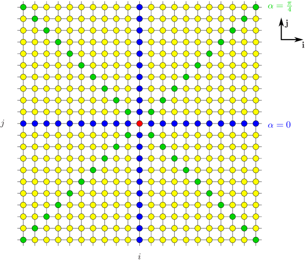
Figure 1: Schematic of the lattice subjected to a point heat source: the particle, where the point heat source is applied, is shown by the red color; two orthogonal rows of the lattice that contain the heat source are shown by the blue color; the main diagonals of the lattice (with respect to the point heat source position) are shown by the green color

The aim of the paper is to develop an equation describing non-stationary heat propagation in the lattice and use this equation to obtain analytical formulas describing the steady-state kinetic temperature distribution caused by a point heat source of a constant intensity. The differences in methodology between the present paper and gavrilov2018heat are:

• When deriving the differential-difference equation describing non-stationary propagation in the lattice, we avoid to use identities of the calculus of finite differences and instead inverse the corresponding finite difference operators, when necessary, in the Fourier domain. This significantly simplifies the formal procedure. Accordingly, we do not introduce into consideration the quantities, which we call “non-local temperatures” in gavrilov2018heat (Section 4) and deal with covariance variables only.

• Since the two-dimensional case is more complicated, the steady-state solution for the kinetic temperature is obtained as a solution of the stationary equations for covariances of the particle velocities (in gavrilov2018heat the steady-state solution was found as a limiting case for the corresponding unsteady solution).

• The investigation of unsteady heat conduction regimes is beyond the scope of this paper.

The paper is organized as follows. In Section 2, we consider the formulation of the problem. In Section 2.1, some general notation is introduced. In Section 2.2, we state the basic equations for the lattice particles in the form of a system of stochastic differential equations. In Section 2.3, we introduce and deal with infinite set of covariance variables. These are the mutual covariances of all the particle velocities and all the displacements for all pairs of particles. We use the Itô lemma to derive (see gavrilov2018heat , Appendix A) an infinite deterministic system of ordinary differential equations which follows from the equations of stochastic dynamics. This system can be transformed into an infinite system of differential-difference equations involving only the covariances for the particle velocities. In Section 3, we introduce a vectorial continuous spatial variable and write the finite difference operators involved in the equation for covariances as compositions of finite difference operators and operators of differentiation. In Section 4, we perform an asymptotic uncoupling of the equation for covariances. Provided that the introduced continuous spatial variable can characterize the behavior of the lattice, one can distinguish between slow motions, which are related to the heat propagation, and vanishing fast motions krivtsov2014energy ; babenkov2016energy ; kuzkin2017high ; Kuzkin-Krivtsov-accepted ; kuzkin2017analytical ; kuzkin2019thermal , which are not considered in the paper. Slow motions can be described by a coupled infinite system of second-order hyperbolic partial differential equations for the continualized covariances of velocities. The kinetic temperature is introduced as a quantity proportional to the variance of the particle velocities. In Section 5 we obtain an analytical expression in the integral form for the steady-state solution describing the kinetic temperature distribution caused by a point source of a constant intensity (the corresponding calculations can be found in Appendices A & B). In Section 6, we present the results of the numerical solution of the initial value problem for the system of stochastic differential equations and compare them with the obtained analytical solution. In the conclusion (Section 7), we discuss the basic results of the paper.

2 Mathematical formulation

2.1 Notation

In the paper, we use the following general notation:

$t$

is the time;

$H(\cdot)$

is the Heaviside function;

$\delta(\cdot)$

is the Dirac delta function in a two-dimensional space;

$\delta_{1}(\cdot)$

is the Dirac delta function in a one-dimensional space;

$\langle\cdot\rangle$

is the expected value for a random quantity;

$\delta_{p;q}$

is the Kronecker delta ($\delta_{p;q}=1$ if $p=q$, and $\delta_{p;q}=0$ otherwise);

$\mathbb{Z}$

is the set of all integers;

$\mathbb{R}$

is the set of all real numbers.

2.2 Stochastic lattice dynamics

Consider the following infinite system of stochastic ordinary differential equations kloeden1999 ; stepanov2013stochastic :

$$\mathrm{d}v_{i,j}=F_{i,j}\,\mathrm{d}t+b_{i,j}\,\mathrm{d}W_{i,j},\qquad\mathrm{d}u_{i,j}=v_{i,j}\,\mathrm{d}t,$$ (2.1)

where

$$F_{i,j}={\color[rgb]{0,0,0}\omega_{0}^{2}{\mathcal{L}}}_{i,j}u_{i,j}-\eta v_{i,j},$$ (2.2)

$$\mathrm{d}W_{i,j}=\rho_{i,j}\sqrt{\mathrm{d}t},$$ (2.3)

$$\omega_{0}\stackrel{{\scriptstyle\mbox{\scriptsize def}}}{{=}}\sqrt{C/m},$$ (2.4)

Here $i,j\in\mathbb{Z}$ are arbitrary integers which describes the position of a particle in the square lattice; the stochastic processes $u_{i,j}(t)$ and $v_{i,j}(t)$ are the displacement and the particle velocity, respectively; $F_{i,j}$ is the force on the particle; $W_{i,j}$ are uncorrelated Wiener processes kloeden1999 ; stepanov2013stochastic ; $b_{i,j}(t)$ is the intensity of the random external excitation; $\eta$ is the specific viscosity for the environment; $C$ is the bond stiffness; $m$ is the mass of a particle; ${\mathcal{L}}_{i,j}$ is the linear finite difference operator describing an infinite two-dimensional stretched square scalar lattice with nearest-neighbor interactions performing out-of-plane vibrations:

$${\mathcal{L}}_{i}u_{i,j}=u_{i+1,j}-2u_{i,j}+u_{i-1,j},$$ (2.5)

$${\mathcal{L}}_{i,j}u_{i,j}={\mathcal{L}}_{i}u_{i,j}+{\mathcal{L}}_{j}u_{i,j}$$ (2.6)

The normal random variables $\rho_{i,j}$ are such that

$$\langle{\rho_{i,j}}\rangle=0,\qquad\langle{\rho_{i,j}\rho_{k,l}}\rangle=\delta_{i;k}\delta_{j;l}$$ (2.7)

and they are assumed to be independent of $u_{i}$ and $v_{i}$. The initial conditions are zero: for all $i$, $j$

$$u_{i,j}(0)=0,\qquad v_{i,j}(0)=0.$$ (2.8)

In the case $b_{i,j}\equiv b$, equations (2.1) are the Langevin equations langevin1908theorie ; lemons1997paul for a two-dimensional harmonic stretched square lattice surrounded by a viscous environment (e.g., a gas or a liquid). Assuming that $b_{i,j}$ may depend on ${i,j}$, we introduce a natural generalization of the Langevin equation which allows one to describe the possibility of an external heat excitation (e.g., laser excitation) gavrilov2018heat . This external excitation is assumed to be localized in space:

$$b_{i,j}\equiv 0\quad\text{if}\quad\max\{i,j\}>R$$ (2.9)

for some $R>0$, and much more intensive than the stochastic influence caused by a non-zero temperature of the environment. Therefore, we neglect in (2.1) the stochastic term, which variance does not depend on $i$ and $j$, that models the influence from the environment. Note that zero initial conditions (2.8) and requirement (2.9) guarantee that there are no sources at the infinity, thus we do not need additional boundary conditions at the infinity.

2.3 The dynamics of covariances

According to (2.2), $F_{i,j}$ are linear functions of $u_{i,j},\ v_{i,j}$. Taking this fact into account together with (2.7) and (2.8), we see that for all $t$

$$\langle{u_{i,j}}\rangle=0,\qquad\langle{v_{i,j}}\rangle=0.$$ (2.10)

Following krivtsov2016ioffe ; gavrilov2018heat , consider the infinite sets of covariance variables

$$\xi_{p,q{;}r,s}\stackrel{{\scriptstyle\mbox{\scriptsize def}}}{{=}}\langle{u_{p,q}\,u_{r,s}}\rangle,\qquad\nu_{p,q{;}r,s}\stackrel{{\scriptstyle\mbox{\scriptsize def}}}{{=}}\langle{u_{p,q}\,v_{r,s}}\rangle,\qquad\kappa_{p,q{;}r,s}\stackrel{{\scriptstyle\mbox{\scriptsize def}}}{{=}}\langle{v_{p,q}\,v_{r,s}}\rangle,$$ (2.11)

and the quantities

$$\beta_{p,q{;}r,s}\stackrel{{\scriptstyle\mbox{\scriptsize def}}}{{=}}\delta_{p;r}\delta_{q;s}\,b_{p,q}b_{r,s}.$$ (2.12)

In the last formula, we take into account the second formula of (2.7). Thus the variables $\xi_{p,q{;}r,s}$, $\nu_{p,q{;}r,s}$, $\kappa_{p,q{;}r,s}$ are defined for any pair of lattice particles. For simplicity, in what follows we drop all the subscripts, i.e., $\xi\stackrel{{\scriptstyle\mbox{\scriptsize def}}}{{=}}\xi_{p,q{;}r,s}$ etc. By definition, we also put $\xi^{\top}\stackrel{{\scriptstyle\mbox{\scriptsize def}}}{{=}}\xi_{r,s{;}p,q}$ etc. Now we differentiate the variables (2.11) with respect to time taking into account the equations of motion (2.1). This yields the following closed system of differential equations for the covariances (see gavrilov2018heat , Appendix A):

$$\begin{gathered}\partial_{t}\xi=\nu+\nu^{\top},\\ \partial_{t}\nu+\eta\nu={\color[rgb]{0,0,0}\omega_{0}^{2}{\mathcal{L}}}_{r,s}\,\xi+\kappa,\\ \partial_{t}\kappa+2\eta\kappa={\color[rgb]{0,0,0}\omega_{0}^{2}{\mathcal{L}}}_{p,q}\nu+{\color[rgb]{0,0,0}\omega_{0}^{2}{\mathcal{L}}}_{r,s}\nu^{\top}+\beta,\end{gathered}$$ (2.13)

where $\partial_{t}$ is the operator of differentiation with respect to time; ${\mathcal{L}}_{p,q}$ and ${\mathcal{L}}_{r,s}$ are the linear difference operators defined by (2.6) that act on $\xi_{p,q{;}r,s}$, $\nu_{p,q{;}r,s}$, $\kappa_{p,q{;}r,s}$, $\beta_{p,q{;}r,s}$ with respect to the first pair of subscripts $p,\ q$ and the second one $r,\ s$, respectively. Now we introduce the symmetric and antisymmetric difference operators

$$2{\mathcal{L}}^{\mathrm{S}}\stackrel{{\scriptstyle\mbox{\scriptsize def}}}{{=}}{\mathcal{L}}_{p,q}+{\mathcal{L}}_{r,s},\qquad 2{\mathcal{L}}^{\mathrm{A}}\stackrel{{\scriptstyle\mbox{\scriptsize def}}}{{=}}{\mathcal{L}}_{p,q}-{\mathcal{L}}_{r,s},$$ (2.14)

and the symmetric and antisymmetric parts of the variable $\nu$:

$$2\nu^{\mathrm{S}}\stackrel{{\scriptstyle\mbox{\scriptsize def}}}{{=}}\nu+\nu^{\top},\qquad 2\nu^{\mathrm{A}}\stackrel{{\scriptstyle\mbox{\scriptsize def}}}{{=}}\nu-\nu^{\top}.$$ (2.15)

Note that $\xi$ and $\kappa$ are symmetric variables. Now equations (2.13) can be rewritten as follows:

$$\partial_{t}\xi=2\nu^{\mathrm{S}},\qquad(\partial_{t}+2\eta)\kappa=2{\color[rgb]{0,0,0}\omega_{0}^{2}{\mathcal{L}}}^{\mathrm{S}}\nu^{\mathrm{S}}+2{\color[rgb]{0,0,0}\omega_{0}^{2}{\mathcal{L}}}^{\mathrm{A}}\nu^{\mathrm{A}}+\beta,$$ (2.16)

$$(\partial_{t}+\eta)\nu^{\mathrm{A}}=-{\color[rgb]{0,0,0}\omega_{0}^{2}{\mathcal{L}}}^{\mathrm{A}}\xi,\qquad(\partial_{t}+\eta)\nu^{\mathrm{S}}={\color[rgb]{0,0,0}\omega_{0}^{2}{\mathcal{L}}}^{\mathrm{S}}\xi+\kappa.$$ (2.17)

This system of equations can be reduced (see gavrilov2018heat ) to one equation of the fourth order in time for covariances of the particle velocities $\kappa$:

$$\left((\partial_{t}+\eta)^{2}(\partial_{t}^{2}+2\eta\partial_{t}-4{\color[rgb]{0,0,0}\omega_{0}^{2}{\mathcal{L}}}^{\mathrm{S}})+4({\color[rgb]{0,0,0}\omega_{0}^{2}{\mathcal{L}}}^{\mathrm{A}})^{2}\right)\kappa=(\partial_{t}+\eta)(\partial_{t}^{2}+\eta\partial_{t}-2{\color[rgb]{0,0,0}\omega_{0}^{2}{\mathcal{L}}}^{\mathrm{S}})\beta.$$ (2.18)

In what follows, we deal with Eq. (2.18). This equation can describe a wide class of systems. For example, in the simplest particular case $\mathscr{L}_{i,j}u_{i,j}=-u_{i,j}$ it can be used to obtain the classical results wang1945theory ; stepanov2013stochastic concerning time evolution of the variance of the velocity for a single stochastic oscillator with additive noise.

According to Eqs. (2.8), (2.11), we supplement Eq. (2.18) with zero initial conditions. We state these conditions in the following form, which is conventional for distributions (or generalized functions) Vladimirov1971 :

$$\kappa\big{|}_{t<0}\equiv 0.$$ (2.19)

To take into account non-zero classical initial conditions, one needs to add the corresponding singular terms (in the form of a linear combination of $\delta(t)$ and its derivatives) to the right-hand sides of the corresponding equations Vladimirov1971 .

Let us note that equation (2.18) is a deterministic equation. What is also important is that (2.18) is a closed equation. Thus, the thermal processes do not depend on any property of the cumulative distribution functions for the displacements and the particle velocities other than the covariance variables used above.

3 Continualization of the finite difference operators

Following krivtsov2015heat ; krivtsov2016ioffe ; gavrilov2018heat , we introduce the discrete spatial variables

$$k\stackrel{{\scriptstyle\mbox{\scriptsize def}}}{{=}}p+r,\qquad l\stackrel{{\scriptstyle\mbox{\scriptsize def}}}{{=}}q+s$$ (3.1)

and the discrete correlational variables

$$m\stackrel{{\scriptstyle\mbox{\scriptsize def}}}{{=}}r-p,\qquad n\stackrel{{\scriptstyle\mbox{\scriptsize def}}}{{=}}s-q.$$ (3.2)

instead of discrete variables $p$, $q$, $r$, $s$. We can also formally introduce the continuous vectorial spatial variable

$$\mathbf{x}\stackrel{{\scriptstyle\mbox{\scriptsize def}}}{{=}}\frac{a}{2}(k\mathbf{i}+l\mathbf{j}),$$ (3.3)

where $a$ is the lattice constant (the distance between neighboring particles along a row), $\mathbf{i}$ and $\mathbf{j}$ are orthogonal unit vectors (the directions of the principal axes of the lattice, see Figure 1). In what follows, we represent $\mathbf{x}$ also in the following form:

$$\mathbf{x}\stackrel{{\scriptstyle\mbox{\scriptsize def}}}{{=}}x_{1}\mathbf{i}+x_{2}\mathbf{j},$$ (3.4)

where $x_{1},\ x_{2}$ are the spatial coordinates in the lattice.

To perform the continualization, we assume that the lattice constant is a small quantity and introduce a dimensionless formal small parameter $\epsilon$ in the following way:

$$a=\epsilon\bar{a},$$ (3.5)

where $\bar{a}=O(1)$. To preserve the speed of sound in the lattice

$$c\stackrel{{\scriptstyle\mbox{\scriptsize def}}}{{=}}a\omega_{0}$$ (3.6)

as a quantity of order $O(1)$, we additionally assume that

$$\omega_{0}=\epsilon^{-1}\bar{\omega}_{0},$$ (3.7)

where $\bar{\omega}_{0}=O(1)$. Thus $c=\bar{a}\bar{\omega}_{0}=O(1)$. The basic assumption that allows one to perform the continualization is that any quantity $\zeta_{p,q{;}r,s}$ defined by (2.11) or (2.12) can be calculated as a value of a smooth function $\hat{\zeta}_{m,n}(\mathbf{x})$ of the continuous spatial slowly varying coordinate $\mathbf{x}=\tfrac{1}{2}\epsilon\bar{a}(k\mathbf{i}+l\mathbf{j})$ and the discrete correlational variables $m$ and $n$:

$$\hat{\zeta}_{m,n}(\mathbf{x})=\zeta_{p,q{;}r,s}.$$ (3.8)

In accordance with Eqs. (3.1), (3.2), one has

$${\mathcal{L}}_{p,q}\zeta_{p,q{;}r,s}= \hat{\zeta}_{m-1,n}\left(\mathbf{x}+\tfrac{a}{2}\mathbf{i}\right)+\hat{\zeta}_{m+1,n}\left(\mathbf{x}-\tfrac{a}{2}\mathbf{i}\right)$$ (3.9)

$$+ \hat{\zeta}_{m,n-1}\left(\mathbf{x}+\tfrac{a}{2}\mathbf{j}\right)+\hat{\zeta}_{m,n+1}\left(\mathbf{x}-\tfrac{a}{2}\mathbf{j}\right)-4\hat{\zeta}_{m,n}(\mathbf{x}),$$

$${\mathcal{L}}_{r,s}\zeta_{p,q{;}r,s}= \hat{\zeta}_{m+1,n}\left(\mathbf{x}+\tfrac{a}{2}\mathbf{i}\right)+\hat{\zeta}_{m-1,n}\left(\mathbf{x}-\tfrac{a}{2}\mathbf{i}\right)$$

$$+ \hat{\zeta}_{m,n+1}\left(\mathbf{x}+\tfrac{a}{2}\mathbf{j}\right)+\hat{\zeta}_{m,n-1}\left(\mathbf{x}-\tfrac{a}{2}\mathbf{j}\right)-4\hat{\zeta}_{m,n}(\mathbf{x}).$$

Applying the Taylor theorem to these formulas yields

$${\mathcal{L}}_{p,q}\zeta_{p,q{;}r,s}={\mathcal{L}}_{m,n}\hat{\zeta}_{m,n} + \tfrac{a}{2}\,\partial_{x_{1}}(\hat{\zeta}_{m-1,n}-\hat{\zeta}_{m+1,n})$$ (3.10)

$$+ \tfrac{a}{2}\,\partial_{x_{2}}(\hat{\zeta}_{m,n-1}-\hat{\zeta}_{m,n+1})+o(\epsilon^{2}),$$

$${\mathcal{L}}_{r,s}\zeta_{p,q{;}r,s}={\mathcal{L}}_{m,n}\hat{\zeta}_{m,n} + \tfrac{a}{2}\,\partial_{x_{1}}(\hat{\zeta}_{m+1,n}-\hat{\zeta}_{m-1,n})$$

$$+ \tfrac{a}{2}\,\partial_{x_{2}}(\hat{\zeta}_{m,n+1}-\hat{\zeta}_{m,n-1})+o(\epsilon^{2}).$$

An alternative way of continualization can be realized by letting the number of particles diverge, rather than invoking an increasingly small separation lepri2010nonequilibrium . Despite the algorithmic difference, these approaches apparently lead to the same result, although application of the first approach to an infinite system seems to be more straightforward.

Now we perform the continualization of the operators ${\mathcal{L}}^{\mathrm{S}},\ {\mathcal{L}}^{\mathrm{A}}$. Using (3.10), we obtain

$${\mathcal{L}}^{\mathrm{S}}={\mathcal{L}}_{m,n}+O(\epsilon^{2}),$$ (3.11)

$${\mathcal{L}}^{\mathrm{A}}=-\tfrac{a}{2}\,\mathscr{D}_{m}\partial_{x_{1}}-\tfrac{a}{2}\,\mathscr{D}_{n}\partial_{x_{2}}+O(\epsilon^{2}).$$ (3.12)

where

$$\mathscr{D}_{n}f_{n}=f_{n+1}-f_{n-1}.$$ (3.13)

4 Slow motions

Taking into account assumption (3.7), Eq. (2.18) can be rewritten in the following form:

$$\bigg{(}(\partial_{t}+\eta)^{2}\big{(}\epsilon^{2}(\partial_{t}^{2}+2\eta\partial_{t})-4\bar{\omega}_{0}^{2}{\mathcal{L}}^{\mathrm{S}}\big{)}+4\frac{\bar{\omega}_{0}^{4}}{\epsilon^{2}}({\mathcal{L}}^{\mathrm{A}})^{2}\bigg{)}\kappa\\ =(\partial_{t}+\eta)\big{(}\epsilon^{2}(\partial_{t}^{2}+\eta\partial_{t})-2\bar{\omega}_{0}^{2}{\mathcal{L}}^{\mathrm{S}}\big{)}\beta.$$ (4.1)

Equation (4.1) is a differential equation whose highest derivative with respect to $t$ is multiplied by a small parameter. Therefore, one can expect the existence of two types of solutions, namely, solutions slowly varying in time and fast varying in time nayfeh2008perturbation ; kevorkian2012multiple . The presence of fast and slow motions is a standard property of statistical systems. Fast motions are oscillations of temperature caused by equilibration of kinetic and potential energies. Slow motions are related with macroscopic heat propagation.

Considering slow motions, we assume that

$$\epsilon^{2}(\partial_{t}^{2}+2\eta\partial_{t})\kappa\ll\bar{\omega}_{0}^{2}{\mathcal{L}}^{\mathrm{S}}\kappa,\qquad\epsilon^{2}(\partial_{t}^{2}+\eta\partial_{t})\beta\ll\bar{\omega}_{0}^{2}{\mathcal{L}}^{\mathrm{S}}\beta.$$ (4.2)

Vanishing solutions krivtsov2014energy ; babenkov2016energy ; kuzkin2017high ; Kuzkin-Krivtsov-accepted ; kuzkin2017analytical that characterize fast motions, which do not satisfy (4.2), are not considered in this paper.

Now, taking into account Eqs. (3.11), (3.12), we drop the higher order terms and rewrite equation (4.1) in the form of an equation for slow motions:

$$\Big{(}(\partial_{t}+\eta)^{2}{\mathcal{L}}_{m\,n}-\tfrac{c^{2}}{4}\big{(}\mathscr{D}_{m}\partial_{x_{1}}+\mathscr{D}_{n}\partial_{x_{2}}\big{)}^{2}\Big{)}\hat{\kappa}_{m,n}=\frac{1}{2}(\partial_{t}+\eta){\mathcal{L}}_{m,n}\hat{\beta}_{m,n},$$ (4.3)

where quantity $\hat{\beta}_{m,n}(\mathbf{x})$ is introduced in accordance with Eq. (3.8). Note that according to (2.12), $\hat{\beta}_{m,n}=0$ if $m\neq 0$ or $n\neq 0$, thus

$$\hat{\beta}_{m,n}=\hat{\beta}_{0,0}(\mathbf{x})\delta_{m;0}\delta_{n;0}.$$ (4.4)

We identify the following quantities depending on the continuous variable $\mathbf{x}$

$$T\equiv\theta_{0,0}(x,t)\stackrel{{\scriptstyle\mbox{\scriptsize def}}}{{=}}mk_{B}^{-1}\hat{\kappa}_{0,0}(\mathbf{x},t),$$ (4.5)

$$\chi(\mathbf{x},t)\stackrel{{\scriptstyle\mbox{\scriptsize def}}}{{=}}\tfrac{1}{2}mk_{B}^{-1}\hat{\beta}_{0,0}(\mathbf{x},t).$$ (4.6)

as the kinetic temperature and the heat supply intensity, respectively. Here $k_{B}$ is the Boltzmann constant. We also introduce the following notation:

$$\theta_{m,n}(x,t)\stackrel{{\scriptstyle\mbox{\scriptsize def}}}{{=}}mk_{B}^{-1}\hat{\kappa}_{m,n}(\mathbf{x},t).$$ (4.7)

Now Eq. (4.3) can be rewritten as the following infinite system of PDE describing non-stationary heat propagation in the lattice:

$$\Big{(}(\partial_{t}+\eta)^{2}{\mathcal{L}}_{m,n}-\tfrac{c^{2}}{4}\big{(}\mathscr{D}_{m}\partial_{x_{1}}+\mathscr{D}_{n}\partial_{x_{2}}\big{)}^{2}\Big{)}\,\theta_{m,n}=(\partial_{t}\chi+\eta\chi){\mathcal{L}}_{m,n}\delta_{m;0}\delta_{n;0}.$$ (4.8)

The initial conditions that corresponds to Eq. (2.19) are

$$\theta_{m,n}(\mathbf{x},t)\big{|}_{t<0}\equiv 0.$$ (4.9)

In the particular case where $\eta=0,\ \chi\propto\delta(t)$, system (4.8) was obtained and investigated in Kuzkin-Krivtsov-accepted . In the latter case the derivation of the corresponding system of PDE is much simpler, since it can be based on consideration of system of ordinary differential equations with random initial conditions instead of system of stochastic equations (2.1).

Note that equations (4.8) for slow motions involve only the product $c=\omega_{0}a$ and do not involve the quantities $\omega_{0}$ and $a$ separately, so they do not involve $\epsilon$. Provided that the initial conditions also do not involve $\epsilon$, the solution of the corresponding initial value problem and all its derivatives are quantities of order $O(1)$. The rate of vanishing for fast motions depends on $\epsilon$: the smaller $\epsilon$, the higher the rate. Thus, for sufficiently small $\epsilon$, exact solutions of Eq. (2.18) quickly transform into slow motions.

5 The steady-state solution of equation for slow motions

In what follows, we look for the steady-state solution of initial value problem for system of partial differential equations (4.8) where the heat supply is given in the form of a point source of a constant intensity. Accordingly, we take

$$\chi={\bar{\chi}_{0}}H(t)\delta(\mathbf{x}),$$ (5.1)

where $\bar{\chi}_{0}=\mathrm{const}$. Looking for the steady-state solution, we substitute $1(t)$ instead of $H(t)$ into Eq. (5.1), replace initial conditions (4.9) by the following boundary condition at infinity

$$\theta_{m,n}\to 0\quad\mathrm{for}\quad\mathbf{x}\to\infty,$$ (5.2)

and drop out the terms involving the time derivatives in (4.8). This yields the following equation

$$\Big{(}\eta^{2}{\mathcal{L}}_{m,n}-\tfrac{c^{2}}{4}\big{(}\mathscr{D}_{m}\partial_{x_{1}}+\mathscr{D}_{n}\partial_{x_{2}}\big{)}^{2}\Big{)}\,\theta_{m,n}=\eta\bar{\chi}_{0}\delta(\mathbf{x}){\mathcal{L}}_{m,n}\delta_{m;0}\delta_{n;0}.$$ (5.3)

Now we apply the discrete Fourier transform with respect to the variables $m,\ n$ to Eq. (5.3):

$$\theta_{{F}}(p_{1},p_{2},\mathbf{x},t)=\sum_{m,n=-\infty}^{\infty}\theta_{m,n}(\mathbf{x})\exp(-\mathrm{i}mp_{1}-\mathrm{i}np_{2}),$$ (5.4)

where subscript $F$ is the symbol of the discrete Fourier transform, $p_{1},\ p_{2}$ are the discrete Fourier transform parameters. Using the shift property for the discrete Fourier transform, one gets

$$\big{(}{\mathcal{L}}_{m\,n}\theta_{m,n}\big{)}_{F}=-4\left({\sin^{2}\frac{p_{1}}{2}+\sin^{2}\frac{p_{2}}{2}}\right)\theta_{F},$$ (5.5)

$$\big{(}\mathscr{D}_{m}\theta_{m,n}\big{)}_{F}=2\mathrm{i}\,\sin{p_{1}}\theta_{F},\qquad\big{(}\mathscr{D}_{n}\theta_{m,n}\big{)}_{F}=2\mathrm{i}\,\sin{p_{2}}\theta_{F},$$ (5.6)

$$\big{(}(\mathscr{D}_{m}\partial_{x_{1}}+\mathscr{D}_{n}\partial_{x_{2}})\theta_{m,n}\big{)}_{F}=2\mathrm{i}\,({\sin p_{1}\mathbf{i}+\sin p_{2}\mathbf{j}})\cdot\nabla\theta_{F},$$ (5.7)

$$(\delta_{m;0}\delta_{n;0})_{F}=1,$$ (5.8)

where

$$\nabla=\partial_{x_{1}}\mathbf{i}+\partial_{x_{2}}\mathbf{j},$$ (5.9)

and dot stands for the scalar product. Multiplying the both sides of the transformed equation (5.3) on $\big{(}{\mathcal{L}}_{m\,n}\big{)}_{F}^{-1}$ results in the following equation:

$$\eta^{2}\theta_{F}-(\boldsymbol{\mathscr{C}}\cdot\nabla)^{2}\theta_{F}=\eta\bar{\chi}_{0}\delta(\mathbf{x})$$ (5.10)

wherein

$$\boldsymbol{\mathscr{C}}={\mathscr{C}_{0}}({\sin p_{1}\mathbf{i}+\sin p_{2}\mathbf{j}}),$$ (5.11)

$${\mathscr{C}_{0}}=\frac{c}{2\sqrt{\sin^{2}\frac{p_{1}}{2}+\sin^{2}\frac{p_{2}}{2}}}.$$ (5.12)

Vector $\boldsymbol{\mathscr{C}}$ coincides with Kuzkin-Krivtsov-accepted the group velocity in the lattice under condition of zero dissipation $\eta=0$.

Thus, Eq. (5.10) describes the steady-state distribution for the Fourier images of the quantities $\theta_{m,n}$ defined by Eq. (4.7) (in particular, the kinetic temperature $T\equiv\theta_{0,0}$), caused by a point heat source of a constant intensity. According to conditions (5.2), Eq. (5.10) should be supplemented with the following boundary condition:

$$\theta_{F}\to 0\quad\mathrm{for}\quad\mathbf{x}\to\infty.$$ (5.13)

Equation (5.10) can be rewritten as

$$\eta^{2}\theta_{F}-(\boldsymbol{\mathscr{C}}\cdot\boldsymbol{\mathscr{C}})(\breve{\boldsymbol{\mathscr{C}}}\cdot\nabla)^{2}\theta_{F}=\bar{\chi}_{0}\eta\delta(\mathbf{x}).$$ (5.14)

Here and in what follows,

$$\breve{\mathbf{a}}=\frac{\mathbf{a}}{|\mathbf{a}|}$$ (5.15)

for any non-zero vector $\mathbf{a}$,

$$\breve{\mathbf{a}}_{\perp}=(\mathbf{i}\times\mathbf{j})\times\breve{\mathbf{a}}$$ (5.16)

for any unit vector $\breve{\mathbf{a}}$, $\times$ is the cross product. Delta-function in the right-hand side of (5.14) can be represented as

$$\delta(\mathbf{x})=\delta_{1}(x_{1})\,\delta_{1}(x_{2})=\delta_{1}(\mathbf{x}\cdot{\breve{\mathbf{n}}})\,\delta_{1}(\mathbf{x}\cdot{\breve{\mathbf{n}}}_{\perp}),$$ (5.17)

where $\breve{\mathbf{n}}$ is an arbitrary unit vector such that

$$\breve{\mathbf{n}}\cdot(\mathbf{i}\times\mathbf{j})=0.$$ (5.18)

We introduce angular variable $\alpha=\arctan\frac{x_{2}}{x_{1}}$ such that

$$\mathbf{x}=|\mathbf{x}|(\cos\alpha\,\mathbf{i}+\sin\alpha\,\mathbf{j}).$$ (5.19)

Due to symmetry, without loss of generality we can assume that (see Figure 1)

$$0\leq\alpha\leq\pi/4.$$ (5.20)

The solution of (5.14) satisfying (5.13) is

$$\theta_{F}=\frac{\bar{\chi}_{0}}{2|\boldsymbol{\mathscr{C}}|}\exp\Big{(}-\frac{\eta}{|\boldsymbol{\mathscr{C}}|}\,|\mathbf{x}\cdot\breve{\boldsymbol{\mathscr{C}}}|\Big{)}\,\delta_{1}(\mathbf{x}\cdot\breve{\boldsymbol{\mathscr{C}}}_{\perp})=\frac{\bar{\chi}_{0}}{2|\mathbf{x}|}\exp\Big{(}-\frac{\eta}{|\boldsymbol{\mathscr{C}}|}\,|\mathbf{x}\cdot\breve{\boldsymbol{\mathscr{C}}}|\Big{)}\,\delta_{1}(\breve{\mathbf{x}}_{\perp}\cdot{\boldsymbol{\mathscr{C}}}).$$ (5.21)

Here we have used Eq. (5.17) wherein $\breve{\mathbf{n}}=\breve{\boldsymbol{\mathscr{C}}}$, and the following formulas:

$$\delta_{1}(Ay)=\frac{1}{|A|}\delta_{1}(y),\qquad A\in\mathbb{R},\ A\neq 0;$$ (5.22)

$$\mathbf{x}\cdot\breve{\boldsymbol{\mathscr{C}}}_{\perp}=0\quad\Longleftrightarrow\quad\breve{\mathbf{x}}_{\perp}\cdot{\boldsymbol{\mathscr{C}}}=0.$$ (5.23)

Applying the inverse Fourier transform, one get the expression for the kinetic temperature $T=\theta_{0,0}$:

$$T=\frac{1}{4\pi^{2}}\iint_{-\pi}^{\pi}\theta_{{F}}\exp(\mathrm{i}mp_{1}+\mathrm{i}np_{2})\,\mathrm{d}y\,\bigg{|}_{m=n=0}\\ =\frac{1}{4\pi^{2}}\,\frac{\bar{\chi}_{0}}{2|\mathbf{x}|}\iint_{-\pi}^{\pi}\exp\Big{(}-\frac{\eta}{|\boldsymbol{\mathscr{C}}(p_{1},p_{2})|}\,|\mathbf{x}\cdot\breve{\boldsymbol{\mathscr{C}}}|\Big{)}\,\delta_{1}\big{(}\breve{\mathbf{x}}_{\perp}\cdot{\boldsymbol{\mathscr{C}}(p_{1},p_{2})}\big{)}\,\mathrm{d}p_{1}\,\mathrm{d}p_{2}.$$ (5.24)

Since the integrand in the right-hand side of Eq. (5.24) contains the Dirac delta-function $\delta_{1}$ in one-dimensional space, formula (5.24) can be rewritten in a simpler form involving a single integral (see Appendix A):

$$T=T_{1}+T_{2}\equiv\frac{\bar{\chi}_{0}}{4\pi^{2}|x_{1}|}\sum_{j=1}^{2}\int_{0}^{\pi}\frac{\exp\left(-\eta\left|\frac{x_{1}}{\sin p_{1}\,{{\mathscr{C}_{0}}\big{(}p_{1},p_{2}^{(j)}\big{)}}}\right|\right)}{{\mathscr{C}_{0}}\big{(}p_{1},p_{2}^{(j)}\big{)}\sqrt{1-\tan^{2}\alpha\,\sin^{2}p_{1}}}\,\mathrm{d}p_{1},$$ (5.25)

where ${\mathscr{C}_{0}}\big{(}p_{1},p_{2}^{(j)}\big{)}$ $(j=1,2)$ are defined by Eqs. (A.13), (A.14). If necessary, the far-field asymptotics of the solution (5.25) can be calculated by means of the Laplace method Fedoruk-Saddle .

5.1 The case $\alpha=0$

In the case $\alpha=0$, i.e. for two orthogonal rows of the lattice that contain the heat source located at $\mathbf{x}=\mathbf{0}$ (see Figure 1), it is possible to obtain the solution in a simpler form. This is done in Appendix B. The final result is $T=T_{1}+T_{2}$, where $T_{1}$ and $T_{2}$ are defined by Eqs.  (B.7), (B.9), respectively.

5.2 The case $\alpha=\pi/4$

Consider the particular case $\alpha=\pi/4$, i.e. the main diagonals of the lattice with respect to a point heat source position (see Figure 1). One has

$$\left.\frac{1}{\sqrt{1-\tan^{2}\alpha\sin^{2}p_{1}}}\right|_{\alpha=\frac{\pi}{4}}=\frac{1}{|\cos p_{1}|}\xrightarrow[p_{1}\to\pm\frac{\pi}{2}]{}+\infty,$$ (5.26)

$${\mathscr{C}_{0}}\big{(}p_{1},p_{2}^{(j)}\big{)}\Big{|}_{\alpha=\frac{\pi}{4},\ p_{1}=\pm\frac{\pi}{2}}=\frac{1}{2}\qquad(j=1,2).$$ (5.27)

Thus, the integrands in the right-hand side of (5.25) have non-integrable singularities at $p_{1}=\pm\pi/2$, and therefore $T=+\infty$. In presence of the dissipation, this seems to be a quite unexpected result, which is discussed in Section 6.

5.3 The solution for a row $x_{2}/a=j$

Consider now the distribution of the kinetic temperature over a row of the lattice $x_{2}/a=j\in\mathbb{Z}$. Provided that assumption (5.20) is true, the analytic expression for the stationary distribution of the kinetic temperature $T$ is (5.25), where

$$\tan\alpha=\frac{|x_{2}|}{|x_{1}|},\qquad|x_{2}|<|x_{1}|.$$ (5.28)

For $\alpha>\pi/4$, due to symmetry with respect to the main diagonal, one has

$$T=\frac{\bar{\chi}_{0}}{4\pi^{2}|x_{2}|}\sum_{j=1}^{2}\int_{0}^{\pi}\frac{\exp\left(-\eta\left|\frac{x_{2}}{\sin p_{1}\,{{\mathscr{C}_{0}}\big{(}p_{1},p_{2}^{(j)}\big{)}}}\right|\right)}{{\mathscr{C}_{0}}\big{(}p_{1},p_{2}^{(j)}\big{)}\sqrt{1-\tan^{2}\alpha\,\sin^{2}p_{1}}}\,\mathrm{d}p_{1},$$ (5.29)

where

$$\tan\alpha=\frac{|x_{1}|}{|x_{2}|},\qquad|x_{1}|<|x_{2}|.$$ (5.30)

6 Numerics

In this section, we present the results of the numerical solution of the system of stochastic differential equations (2.1)–(2.3) with initial conditions (2.8). It is useful to rewrite Eqs. (2.1)–(2.3) in the dimensionless form

$$\mathrm{d}{\tilde{v}}_{i,j}=({\mathcal{L}}_{i,j}{\tilde{u}}_{i,j}-\eta{\tilde{v}}_{i,j})\,\mathrm{d}\tilde{t}+\tilde{b}_{i,j}\rho_{i,j}\sqrt{\mathrm{d}\tilde{t}},$$ (6.1)

$$\mathrm{d}{\tilde{u}}_{i,j}={\tilde{v}}_{i,j}\,\mathrm{d}\tilde{t},$$

where

$$\tilde{u}\stackrel{{\scriptstyle\mbox{\scriptsize def}}}{{=}}\frac{u}{a},\quad\tilde{v}\stackrel{{\scriptstyle\mbox{\scriptsize def}}}{{=}}\frac{v}{c},\quad\tilde{t}\stackrel{{\scriptstyle\mbox{\scriptsize def}}}{{=}}{\omega_{0}}t,\quad\tilde{b}\stackrel{{\scriptstyle\mbox{\scriptsize def}}}{{=}}\frac{b}{c\sqrt{\omega_{0}}},\quad\tilde{\eta}\stackrel{{\scriptstyle\mbox{\scriptsize def}}}{{=}}\frac{\eta}{\omega_{0}}.$$ (6.2)

We consider the square lattice of $(2N+1)^{2}$ particles with the following boundary conditions

$$u_{-N,i} =u_{-N+1,i}, u_{N,i}=u_{N-1,i},$$ (6.3)

$$v_{-N,i} =v_{-N+1,i}, v_{N,i}=v_{N-1,i},$$

$$u_{i,-N} =u_{i,-N+1}, u_{i,N}=u_{i,N-1},$$

$$v_{i,-N} =v_{i,-N+1}, v_{i,N}=v_{i,N-1},$$

where $i=\overline{-N,N}$. Actually, the specific form of this boundary conditions is not very important in our calculations, since we take large enough $N$ such that the wave reflections from the boundaries do not occur. To obtain a numerical solution in the case of the point source of the heat supply located at $i=0$, $j=0$, we assume that $\tilde{b}_{i,j}\rho_{i,j}=\delta_{i;0}\delta_{j;0}\tilde{b}\rho_{i,j}$ and use the scheme

$$\Delta{\tilde{v}}_{i,j}^{k} =({\mathcal{L}}_{{i,j}}{\tilde{u}}_{i,j}^{k}-\eta{\tilde{v}}_{i,j}^{k})\Delta{\tilde{t}}+\tilde{b}\delta_{i;0}\delta_{j;0}\rho^{k}_{i,j}\sqrt{\Delta{\tilde{t}}},$$ (6.4)

$$\Delta{\tilde{u}}_{i,j}^{k} ={\tilde{v}}_{i,j}^{k+1}\Delta{\tilde{t}},$$

$$\tilde{v}^{k+1}_{{i,j}} =\tilde{v}^{k}_{{i,j}}+\Delta\tilde{v}^{k}_{{i,j}},$$

$$\tilde{u}^{k+1}_{{i,j}} =\tilde{u}^{k}_{{i,j}}+\Delta\tilde{u}^{k}_{{i,j}},$$

where $i,j=\overline{-N,N}$. Here the symbols with superscript $k$ denote the corresponding quantities at $\tilde{t}=\tilde{t}^{k}\stackrel{{\scriptstyle\mbox{\scriptsize def}}}{{=}}k\Delta\tilde{t}$: ${\tilde{u}}_{i,j}^{k}={\tilde{u}}_{i,j}(\tilde{t}^{k}),\ \tilde{v}_{i,j}^{k}=\tilde{v}_{i,j}(\tilde{t}^{k})$; $\rho^{k}$ are normal random numbers that satisfy (2.7) generated for all $\tilde{t}^{k}$. Without loss of generality we can take $\tilde{b}=1$. Due to symmetry of the problem we can perform the calculations only for $1/8$ of the whole lattice ($i=\overline{0,N}$, $j=\overline{0,i}$).

We perform a series of $r=1\dots R$ realizations of these calculations (with various independent $\rho^{k}_{(r)}$) and get the corresponding particle velocities $\tilde{v}^{k}_{(r)i,j}$. In accordance with (4.5), in order to obtain the dimensionless kinetic temperature

$$\tilde{T}=\frac{Tk_{B}}{mc^{2}},$$ (6.5)

we should average the doubled dimensionless kinetic energies:

$$\tilde{T}_{i,j}^{k}=\frac{1}{R}\sum_{r=1}^{R}(\tilde{v}^{k}_{(r)i,j})^{2}.$$ (6.6)

Numerical results (6.6) for the kinetic temperature can be compared with the analytical steady-state solution (5.25), expressed in the dimensionless form wherein $a=1,\ c=1$, $x_{1}=i$, $x_{2}=j$, and

$$\bar{\chi}_{0}=\frac{\tilde{b}^{2}}{2}.$$ (6.7)

Note that the factor $1/2$ in the right-hand sides of the last formula appears according to Eq. (4.6).

The comparison between analytical and numerical results is presented in Figures 2–6. All calculations were performed for the following values of the problem parameters: $\tilde{\eta}=0.1$, $N=100$, $\tilde{t}=100$, $R=100000$. The time step is $\Delta{\tilde{t}}=0.025$. To perform the numerical calculations we use SciPy software scipy .

In Figure 2 one can see the general view of a central zone of the kinetic temperature distribution pattern in the lattice. One can observe that most of the heat propagates along the main diagonals of the lattice (with respect to a point source position). This result is in a qualitative agreement with results obtained earlier in studies mielke2006macroscopic ; harris2008energy , where energy transport in lattices are discussed in the deterministic case, and also with results of Kuzkin-Krivtsov-accepted .

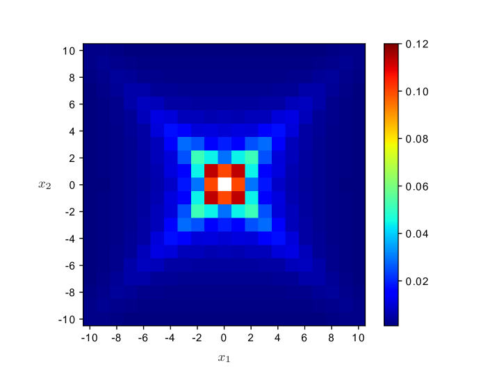
Figure 2: The central zone of the kinetic temperature distribution pattern in a square two-dimensional lattice, caused by a constant point source (the value at the central point $\tilde{T}_{0,0}\simeq 0.79$ is shown by the white color)

In Figure 3 we compare the steady-state analytical solution in the form of Eqs. (B.7), (B.9) for the row $x_{2}=0$ (the blue solid line) and the numerical solution (the red crosses).

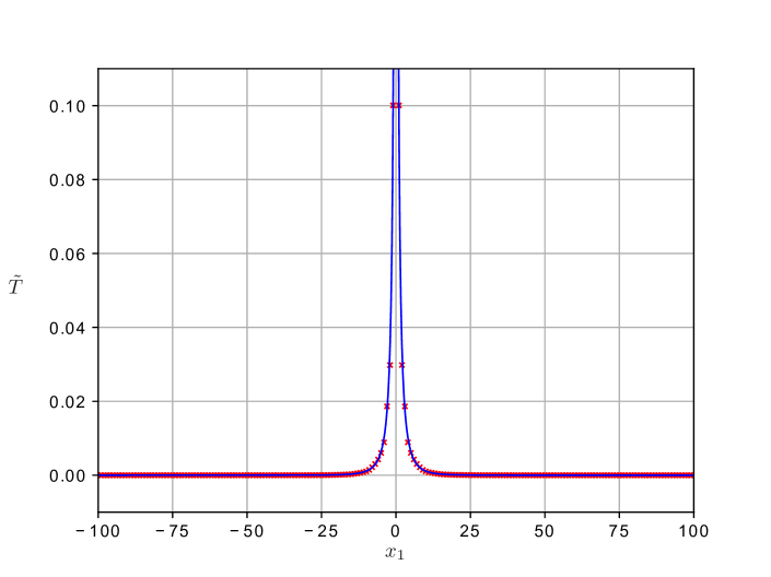
Figure 3: Comparing the steady-state analytical solution in the form of Eqs. (B.7), (B.9) for the row $x_{2}=0$ (the blue solid line) and the numerical solution (the red crosses)

In Figure 4 we compare the steady-state analytical solution in the form of Eqs. (5.25), (5.29) for the row $x_{2}=7$ (the blue solid line) and the numerical solution (the red crosses). The corresponding view of a central zone of the kinetic temperature distribution is given in Figure 5. One can see that numerical value at the point $|x_{1}|=7$ of the lattice at the main diagonal is finite, whereas the analytic continuum solution is singular at this point.

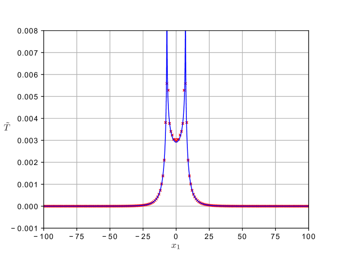
Figure 4: Comparing the steady-state analytical solution in the form of Eqs. (5.25), (5.29) for the row $x_{2}=7$ (the blue solid line) and the numerical solution (the red crosses)

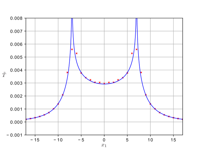
Figure 5: Comparing the steady-state analytical solution in the form of Eqs. (5.25), (5.29) for the central zone of row $x_{2}=7$ (the blue solid line) and the numerical solution (the red crosses)

Finally, in Figure 6 we compare the steady-state analytical solution in the form of Eqs. (5.25), (5.29) for the row $x_{2}=1$ (the blue solid line) and the numerical solution (the red crosses) in a central zone near the source.

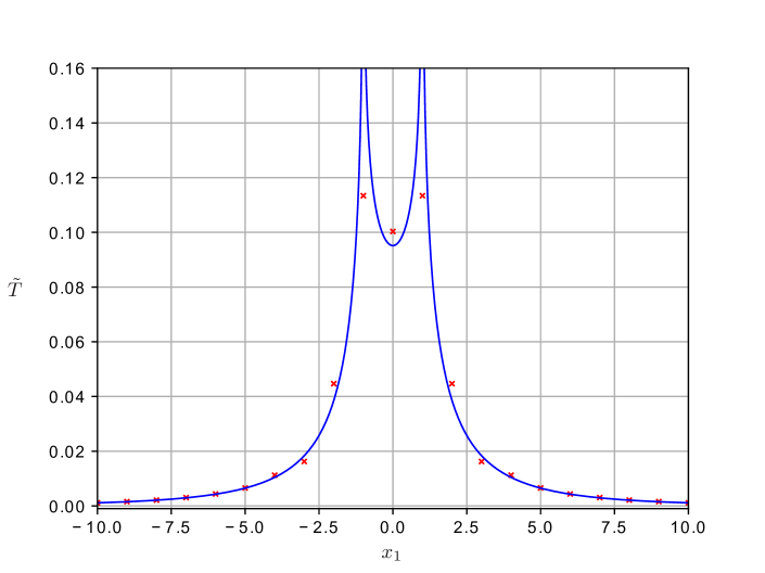
Figure 6: Comparing the steady-state analytical solution in the form of Eqs. (5.25), (5.29) for the central zone of row $x_{2}=1$ (the blue solid line) and the numerical solution (the red crosses)

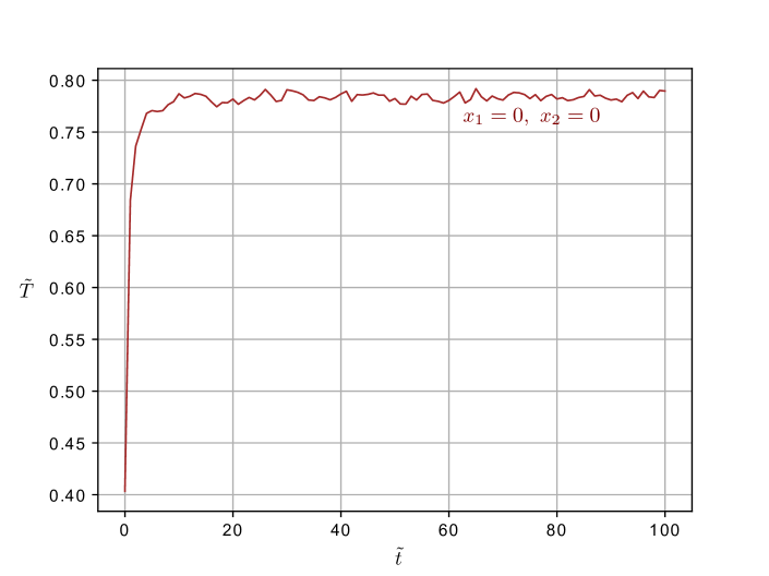
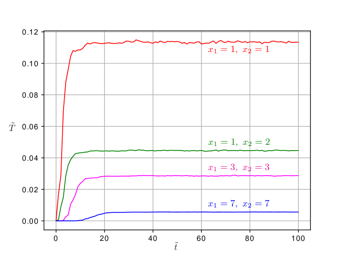
Figure 7: Plots of the numerical solution for the kinetic temperature at several fixed positions versus the time (the plots are drawn with time step $1.0$)

One can see that in all cases, the analytical and numerical solutions are in a very good agreement everywhere except the main diagonals of the lattice $|x_{1}|=|x_{2}|$ (see Figures 3–6). The continuous analytical solution predicts singularities in the stationary solution at the main diagonals (see Section 5.2). Usually, such a result means that a corresponding non-stationary solution grows with time, and a steady-state solution at singular points does not exist. However, the numerical calculations based on the original infinite system of stochastic ODE contradict with such a hypothesis and predict that despite most of the heat propagates along the main diagonals of the lattice (see Figure 2), the kinetic temperature at the main diagonals apparently converges to finite values (see Figure 7, where plots of the numerical solution for the kinetic temperature at several fixed positions versus the time are given). In particular, this is true for the point $x_{1}=x_{2}=0$ where the heat source is located (see Figure 7). Note that in one-dimensional case considered in gavrilov2018heat we also observe the singularity in the continuous solution at the point where heat source is applied, whereas the numerics predicts the finite value of the kinetic temperature at that point. In our opinion, such paradoxical result is caused by the continualization procedure (in particular, by the choice of heat supply intensity in singular form (5.1)), and it definitely needs an additional investigation. Note that in the conservative non-stochastic case the singularities at main diagonals were discovered in mielke2006macroscopic ; harris2008energy ; giannoulis2006continuum , where they are associated with non-smoothness of the dispersion relation.

7 Conclusion

In the paper, we started with equations (2.1) for stochastic dynamics of a two-dimensional harmonic square scalar lattice in a viscous environment. We introduced in the standard way the kinetic temperature in the lattice as a quantity proportional to the variance of the particle velocities. The most important results of the paper are the differential-difference equation (4.8) describing non-stationary heat propagation in the lattice and the analytical formula in the integral form (5.25) describing the steady-state kinetic temperature distribution in the lattice caused by a point heat source of a constant intensity.

The comparison between numerical solution of equations (2.1) and analytic steady-state solution (5.25) of differential-difference equation (4.8) demonstrates a a very good agreement everywhere except the main diagonals of the lattice with respect to the point source position (see Figures 3–6). The continuous analytical solution predicts singularities in the stationary solution at the main diagonals (see Section 5.2), whereas the numerical solution predicts that despite most of the heat propagates along the main diagonals of the lattice (see Figure 2), the kinetic temperature at the main diagonals apparently converges to finite values (see Figure 7). In our opinion, such a paradoxical result can be caused by the continualization procedure (in particular, by the choice of heat supply intensity in singular form (5.1)). Another possible oversimplification in physical modeling that makes the main diagonals to be preferable directions for heat propagation, apparently, is the choice of the potential of interaction involving for a given particle only four neighbours (as it is stated by Eqs. (2.5), (2.6)). This situation needs an additional investigation.

We expect that the results obtained in the paper can be used to describe the heat transfer in low-dimensional nanostructures and ultra-pure materials chang2008breakdown ; xu2014length ; goldstein2007mechanics . The subject of our future work is to generalize the theoretical results to the case of the graphene lattice and to verify the results by means of experiments with the laser heating of graphene hwang2016measuring ; indeitsev2017two .

Appendix A Calculation of the steady-state solution in the integral form

To calculate the right-hand side of Eq. (5.24), one needs to use the formula (see G-Sh-1 )

$$\int_{I}\delta_{1}\big{(}f({y})\big{)}\,\mathrm{d}{y}=\sum_{j}\frac{1}{|f^{\prime}({y}_{j})|}.$$ (A.1)

where $y_{j}$ are the roots of $f(y)$ lying inside the interval $I$.

One has

$$\mathbf{x}_{\perp}=|\mathbf{x}|(\cos\alpha\,\mathbf{j}-\sin\alpha\,\mathbf{i}),$$ (A.2)

$$\breve{\mathbf{x}}_{\perp}\cdot\boldsymbol{\mathscr{C}}={\mathscr{C}_{0}}(\cos\alpha\sin p_{2}-\sin\alpha\sin p_{1}),$$ (A.3)

$$\breve{\mathbf{x}}_{\perp}\cdot\boldsymbol{\mathscr{C}}=0\quad\Longleftrightarrow\quad\cos\alpha\sin p_{2}-\sin\alpha\sin p_{1}=0\quad\Longleftrightarrow\quad\frac{\sin p_{2}}{\sin p_{1}}=\tan\alpha\\ \Longleftrightarrow\quad p_{2}=p_{2}^{(j,k)},\quad j=1,2;\ k\in\mathbb{Z};$$ (A.4)

where

$$\begin{gathered}p_{2}^{(1,k)}\equiv\arcsin(\tan\alpha\sin p_{1})+2\pi k,\\ p_{2}^{(2,k)}\equiv\pi-\arcsin(\tan\alpha\sin p_{1})+2\pi k,\end{gathered}$$ (A.5)

such that $p_{2}^{(j,k)}\in[-\pi,\pi]$. The typical structure of roots $p_{2}^{(j,k)}$ in the case $0<\alpha<\pi/4$ is presented in Figure 8.

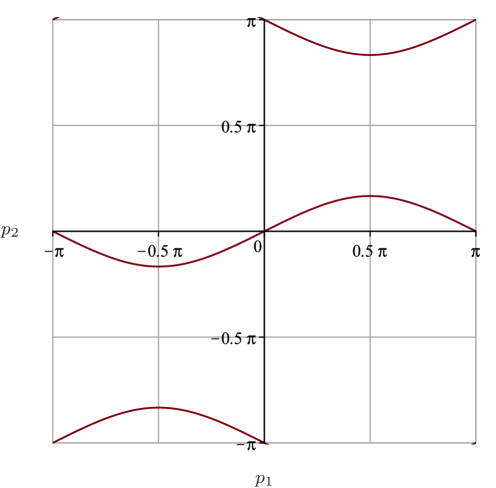
Figure 8: Structure of roots $p_{2}^{(j,k)}$ defined by (A.5) such that $p_{2}^{(j,k)}\in[-\pi,\pi]$ in the case $0<\alpha<\pi/2$ (here $\alpha=\arctan{\tfrac{1}{2}})$

For $p_{1}\neq 0$ there exist exactly two roots lying in the interval $[-\pi,\pi]$. The first one corresponds to the choice $j=1,\ k=0$, and the second one corresponds to the choice $j=2,\ k=0$ for $p_{1}>0$ and $j=2,\ k=-1$ for $p_{1}<0$. Thus, for $0<\alpha<\pi/4$ we put

$$\begin{gathered}p_{2}^{(1)}\equiv\arcsin(\tan\alpha\sin p_{1}),\\ p_{2}^{(2)}\equiv\pm\pi-\arcsin(\tan\alpha\sin p_{1}),\quad\pm p_{1}>0.\end{gathered}$$ (A.6)

Applying now formula (A.1), one gets

$$\delta_{1}(\breve{\mathbf{x}}_{\perp}\cdot\boldsymbol{\mathscr{C}})=\sum_{j=1}^{2}\frac{\delta_{1}\big{(}p_{2}-p_{2}^{(j)}\big{)}}{{\mathscr{C}_{0}}|\cos\alpha|\,\big{|}\cos p_{2}^{(j)}\big{|}},$$ (A.7)

$$T=\sum_{j}T_{j}\equiv\frac{\bar{\chi}_{0}}{8\pi^{2}|\mathbf{x}|\,|\cos\alpha|}\sum_{j=1}^{2}\int_{-\pi}^{\pi}\frac{1}{{\mathscr{C}_{0}}\big{|}\cos p_{2}^{(j)}\big{|}}\,{\exp\left(-\frac{\eta\,|\mathbf{x}\cdot\breve{\boldsymbol{\mathscr{C}}}|}{\big{|}\boldsymbol{\mathscr{C}}\big{|}}\right)}\,\mathrm{d}p_{1}.$$ (A.8)

According to (A.5) one has:

$$\cos\arcsin p=\sqrt{1-p^{2}},$$ (A.9)

$$|\cos p_{2}^{(j)}|=\sqrt{1-\tan^{2}\alpha\,\sin^{2}p_{1}},\quad j=1,2.$$ (A.10)

Using (5.12), and taking into account identities

$$\sin^{2}\frac{p}{2}=\frac{1-\cos p}{2},$$ (A.11)

$$\cos^{2}\alpha=\frac{1}{1+\tan^{2}\alpha},$$ (A.12)

one obtains

$${\mathscr{C}_{0}}\big{(}p_{1},p_{2}^{(1)}\big{)}=\frac{c}{2\sqrt{\sin^{2}\frac{p_{1}}{2}+\frac{1-\cos\arcsin(\tan\alpha\sin p_{1})}{2}}}=\frac{c}{2\sqrt{\sin^{2}\frac{p_{1}}{2}+\frac{1-\sqrt{1-\tan^{2}\alpha\,\sin^{2}p_{1}}}{2}}},$$ (A.13)

$${\mathscr{C}_{0}}\big{(}p_{1},p_{2}^{(2)}\big{)}=\frac{c}{2\sqrt{\sin^{2}\frac{p_{1}}{2}+\frac{1+\cos\arcsin(\tan\alpha\sin p_{1})}{2}}}=\frac{c}{2\sqrt{\sin^{2}\frac{p_{1}}{2}+\frac{1+\sqrt{1-\tan^{2}\alpha\,\sin^{2}p_{1}}}{2}}}.$$ (A.14)

According to (3.4), (5.11), one gets

$$\boldsymbol{\mathscr{C}}\big{(}p_{1},p_{2}^{(j)}\big{)}={\mathscr{C}_{0}}\big{(}p_{1},p_{2}^{(j)}\big{)}\sin p_{1}({\mathbf{i}+\tan\alpha\,\mathbf{j}}),$$ (A.15)

$$\Big{|}\boldsymbol{\mathscr{C}}\big{(}p_{1},p_{2}^{(j)}\big{)}\Big{|}={\mathscr{C}_{0}}\big{(}p_{1},p_{2}^{(j)}\big{)}|\sin p_{1}|\sqrt{1+\tan^{2}\alpha},$$ (A.16)

$$\breve{\boldsymbol{\mathscr{C}}}\big{(}p_{1},p_{2}^{(j)}\big{)}=\frac{\operatorname{sign}p_{1}}{\sqrt{1+\tan^{2}\alpha}}\,{(\mathbf{i}+\tan\alpha\,\mathbf{j})},$$ (A.17)

$$\mathbf{x}=x_{1}(\mathbf{i}+\tan\alpha\,\mathbf{j}),$$ (A.18)

$$\mathbf{x}\cdot\breve{\boldsymbol{\mathscr{C}}}\big{(}p_{1},p_{2}^{(j)}\big{)}={x_{1}\operatorname{sign}p_{1}}{\sqrt{1+\tan^{2}\alpha}},$$ (A.19)

$$\frac{\Big{|}\mathbf{x}\cdot\breve{\boldsymbol{\mathscr{C}}}\big{(}p_{1},p_{2}^{(j)}\big{)}\Big{|}}{\Big{|}\boldsymbol{\mathscr{C}}\big{(}p_{1},p_{2}^{(j)}\big{)}\Big{|}}=\left|\frac{x_{1}}{\sin p_{1}\,{{\mathscr{C}_{0}}\big{(}p_{1},p_{2}^{(j)}\big{)}}}\right|,$$ (A.20)

$$|\mathbf{x}|=\sqrt{x_{1}^{2}+x_{2}^{2}}=|x_{1}|\sqrt{1+\tan^{2}\alpha},$$ (A.21)

$$|\mathbf{x}|\,|\cos\alpha|=|x_{1}|,$$ (A.22)

where $j=1,2$. Finally, substituting of these expressions into Eq. (A.8) and simplifying of expression obtained, results in the formula for the solution in the solution in the integral form:

$$T=T_{1}+T_{2}=\frac{\bar{\chi}_{0}}{4\pi^{2}|x_{1}|}\sum_{j=1}^{2}\int_{0}^{\pi}\frac{\exp\left(-\eta\left|\frac{x_{1}}{\sin p_{1}\,{{\mathscr{C}_{0}}\big{(}p_{1},p_{2}^{(j)}\big{)}}}\right|\right)}{{\mathscr{C}_{0}}\big{(}p_{1},p_{2}^{(j)}\big{)}\sqrt{1-\tan^{2}\alpha\,\sin^{2}p_{1}}}\,\mathrm{d}p_{1},$$ (A.23)

Appendix B Calculation of the steady-state solution in the particular case $\alpha=0$

In the case under consideration, due to (A.5) one has

$$\begin{gathered}p_{2}^{(1,0)}=0,\\ p_{2}^{(2,0)}=\pi,\qquad p_{2}^{(2,-1)}=-\pi.\end{gathered}$$ (B.1)

Since in the case $p=p_{2}$ the roots lie at the boundaries of the interval $[-\pi,\pi]$, we take the corresponding contributions multiplied by $1/2$. Since these contributions are equal to each other, we can put

$$\begin{gathered}p_{2}^{(1)}=0,\\ p_{2}^{(2)}=\pi\end{gathered}$$ (B.2)

and use the formulas obtained above. According to Eqs. (A.13), (A.14) one gets

$${\mathscr{C}_{0}}\big{(}p_{1},p_{2}^{(1)}\big{)}=\frac{c}{2|\sin\frac{p_{1}}{2}|},$$ (B.3)

$${\mathscr{C}_{0}}\big{(}p_{1},p_{2}^{(2)}\big{)}=\frac{c}{2\sqrt{\sin^{2}\frac{p_{1}}{2}+1}},$$ (B.4)

Thus,

$$T_{1}=\frac{\bar{\chi}_{0}}{4\pi^{2}{|x_{1}|}}\int_{0}^{\pi}\frac{2}{c}\left|\sin\frac{p_{1}}{2}\right|\,{\exp\left(-\frac{\eta{|x_{1}|}}{c\left|\cos\frac{p_{1}}{2}\right|}\right)}\,\mathrm{d}p_{1}=\frac{\bar{\chi}_{0}}{\pi^{2}{|x_{1}|}c}\int_{0}^{\pi/2}\sin y\,{\exp\left(-\frac{\eta{|x_{1}|}}{c\cos y}\right)}\,\mathrm{d}y.$$ (B.5)

Let $\gamma=\frac{1}{\cos y}$. One has

$$\mathrm{d}\gamma=\frac{\sin y}{\cos^{2}y}\,\mathrm{d}y=\gamma^{2}\sin y\,\mathrm{d}y,$$ (B.6)

and, therefore,

$$T_{1}=\frac{\bar{\chi}_{0}}{\pi^{2}{|x_{1}|}c}\int_{1}^{\infty}\gamma^{-2}\,{\exp\left(-\frac{\eta{|x_{1}|}\gamma}{c}\right)}\,\mathrm{d}\gamma=\frac{\bar{\chi}_{0}}{\pi^{2}{|x_{1}|}c}\left(\exp\left(-\frac{\eta{|x_{1}|}}{c}\right)-\frac{\eta{|x_{1}|}}{c}\operatorname{E}_{1}\left(\frac{\eta{|x_{1}|}}{c}\right)\right),$$ (B.7)

where

$$\operatorname{E}_{1}(z)=\int_{1}^{\infty}\frac{\exp(-\gamma z)}{\gamma}\,\mathrm{d}\gamma,\quad\operatorname{Re}(z)>0$$ (B.8)

is the exponential integral abramowitz1972handbook . For $T_{2}$ one gets the solution in the integral form

$$T_{2}=\frac{\bar{\chi}_{0}}{2\pi^{2}{|x_{1}|}c}\int_{0}^{\pi}\sqrt{\sin^{2}\frac{p_{1}}{2}+1}\,\,{\exp\left(-\frac{2\eta{|x_{1}|}\sqrt{\sin^{2}\frac{p_{1}}{2}+1}}{c\sin{p_{1}}}\right)}\,\mathrm{d}p_{1}.$$ (B.9)

References

- (1) Chang, C., Okawa, D., Garcia, H., Majumdar, A., Zettl, A.: Breakdown of Fourier’s law in nanotube thermal conductors. Physical review letters 101(7), 075,903 (2008)
- (2) Xu, X., Pereira, L., Wang, Y., Wu, J., Zhang, K., Zhao, X., Bae, S., Bui, C., Xie, R., Thong, J., Hong, B., Loh, K., Donadio, D., Li, B., Özyilmaz, B.: Length-dependent thermal conductivity in suspended single-layer graphene. Nature communications 5 (2014)
- (3) Hsiao, T., Huang, B., Chang, H., Liou, S., Chu, M., Lee, S., Chang, C.: Micron-scale ballistic thermal conduction and suppressed thermal conductivity in heterogeneously interfaced nanowires. Physical Review B 91(3), 035,406 (2015)
- (4) Cahill, D., Ford, W., Goodson, K., Mahan, G., Majumdar, A., Maris, H., Merlin, R., Phillpot, S.: Nanoscale thermal transport. Journal of Applied Physics 93(2), 793–818 (2003)
- (5) Liu, S., Xu, X., Xie, R., Zhang, G., Li, B.: Anomalous heat conduction and anomalous diffusion in low dimensional nanoscale systems. The European Physical Journal B 85(337) (2012)
- (6) Chang, C.: Experimental probing of non-Fourier thermal conductors. In: S. Lepri (ed.) Thermal transport in low dimensions: from statistical physics to nanoscale heat transfer, Lecture Notes in Physics, vol. 921, pp. 305–338. Springer (2016)
- (7) Lepri, S., Livi, R., Politi, A.: Thermal conduction in classical low-dimensional lattices. Physics reports 377(1), 1–80 (2003)
- (8) Spohn, H.: Fluctuating hydrodynamics approach to equilibrium time correlations for anharmonic chains. In: S. Lepri (ed.) Thermal transport in low dimensions: from statistical physics to nanoscale heat transfer, Lecture Notes in Physics, pp. 107–158. Springer (2016)
- (9) Hoover, W., Hoover, C.: Simulation and Control of Chaotic Nonequilibrium Systems. World Scientific (2015)
- (10) Daly, B., Maris, H., Imamura, K., Tamura, S.: Molecular dynamics calculation of the thermal conductivity of superlattices. Physical review B 66(2), 024,301 (2002)
- (11) Krivtsov, A.: From nonlinear oscillations to equation of state in simple discrete systems. Chaos, Solitons & Fractals 17(1), 79–87 (2003)
- (12) Berinskii, I.: Elastic networks to model auxetic properties of cellular materials. International Journal of Mechanical Sciences 115, 481–488 (2016)
- (13) Kuzkin, V., Krivtsov, A., Podolskaya, E., Kachanov, M.: Lattice with vacancies: elastic fields and effective properties in frameworks of discrete and continuum models. Philosophical Magazine 96(15), 1538–1555 (2016)
- (14) Berinskii, I., Krivtsov, A.: Linear oscillations of suspended graphene. In: Shell and Membrane Theories in Mechanics and Biology, pp. 99–107. Springer (2015)
- (15) Berinskii, I., Krivtsov, A.: A hyperboloid structure as a mechanical model of the carbon bond. International Journal of Solids and Structures 96, 145–152 (2016)
- (16) Bonetto, F., Lebowitz, J., Rey-Bellet, L.: Fourier’s law: A challenge to theorists. In: A. Fokas, A. Grigoryan, T. Kibble, B. Zegarlinski (eds.) Mathematical physics 2000. World Scientific (2000)
- (17) Lepri, S., Livi, R., Politi, A.: On the anomalous thermal conductivity of one-dimensional lattices. Europhysics Letters 43(3), 271 (1998)
- (18) Dhar, A.: Heat transport in low-dimensional systems. Advances in Physics 57(5), 457–537 (2008)
- (19) Rieder, Z., Lebowitz, J., Lieb, E.: Properties of a harmonic crystal in a stationary nonequilibrium state. Journal of Mathematical Physics 8(5), 1073–1078 (1967)
- (20) Allen, K., Ford, J.: Energy transport for a three-dimensional harmonic crystal. Physical Review 187(3), 1132 (1969)
- (21) Nakazawa, H.: On the lattice thermal conduction. Progress of Theoretical Physics Supplement 45, 231–262 (1970)
- (22) Lee, L., Dhar, A.: Heat conduction in a two-dimensional harmonic crystal with disorder. Physical review letters 95(9), 094,302 (2005)
- (23) Kundu, A., Chaudhuri, A., Roy, D., Dhar, A., Lebowitz, J., Spohn, H.: Heat conduction and phonon localization in disordered harmonic crystals. Europhysics Letters 90(4), 40,001 (2010)
- (24) Dhar, A., Saito, K.: Heat transport in harmonic systems. In: S. Lepri (ed.) Thermal transport in low dimensions: from statistical physics to nanoscale heat transfer, Lecture Notes in Physics, vol. 921, pp. 39–106. Springer (2016)
- (25) Bernardin, C., Kannan, V., Lebowitz, J., Lukkarinen, J.: Harmonic systems with bulk noises. Journal of Statistical Physics 146(4), 800–831 (2012)
- (26) Freitas, N., Paz, J.: Analytic solution for heat flow through a general harmonic network. Physical Review E 90(4), 042,128 (2014)
- (27) Freitas, N., Paz, J.: Erratum: Analytic solution for heat flow through a general harmonic network. Physical Review E 90(6), 069,903 (2014)
- (28) Hoover, W., Hoover, C.: Hamiltonian thermostats fail to promote heat flow. Communications in Nonlinear Science and Numerical Simulation 18(12), 3365–3372 (2013)
- (29) Lukkarinen, J., Marcozzi, M., Nota, A.: Harmonic chain with velocity flips: thermalization and kinetic theory. Journal of Statistical Physics 165(5), 809–844 (2016)
- (30) Le-Zakharov, A., Krivtsov, A.: Molecular dynamics investigation of heat conduction in crystals with defects. Doklady Physics 53(5), 261–264 (2008)
- (31) Gendelman, O., Shvartsman, R., Madar, B., Savin, A.: Nonstationary heat conduction in one-dimensional models with substrate potential. Physical Review E 85(1), 011,105 (2012)
- (32) Tsai, D., MacDonald, R.: Molecular-dynamical study of second sound in a solid excited by a strong heat pulse. Physical Review B 14(10), 4714 (1976)
- (33) Ladd, A., Moran, B., Hoover, W.: Lattice thermal conductivity: A comparison of molecular dynamics and anharmonic lattice dynamics. Physical Review B 34(8), 5058 (1986)
- (34) Volz, S., Saulnier, J.B., Lallemand, M., Perrin, B., Depondt, P., Mareschal, M.: Transient Fourier-law deviation by molecular dynamics in solid argon. Physical review B 54(1), 340 (1996)
- (35) Gendelman, O., Savin, A.: Nonstationary heat conduction in one-dimensional chains with conserved momentum. Physical Review E 81(2), 020,103 (2010)
- (36) Guzev, M.: The exact formula for the temperature of a one-dimensional crystal. Far Eastern Mathematical Journal 18(1), 39–47 (2018)
- (37) Krivtsov, A.: Energy oscillations in a one-dimensional crystal. Doklady Physics 59(9), 427–430 (2014)
- (38) Krivtsov, A.: Heat transfer in infinite harmonic one-dimensional crystals. Doklady Physics 60(9), 407–411 (2015)
- (39) Krivtsov, A.: The ballistic heat equation for a one-dimensional harmonic crystal. In: H. Altenbach, et al. (eds.) Dynamical Processes in Generalized Continua and Structures, Advanced Structured Materials 103, pp. 345–358. Springer (2019). DOI 10.1007/978-3-030-11665-1˙19
- (40) Chandrasekharalah, D.: Thermoelasticity with second sound: a review. Appl. Mech. Rev. 39(3), 355 (1986)
- (41) Tzou, D.: Macro-to microscale heat transfer: the lagging behavior. John Wiley & Sons (2014)
- (42) Cattaneo, C.: Sur une forme de l’équation de la chaleur éliminant le paradoxe d’une propagation instantanée. Comptes Rendus de L’Academie des Sciences 247(4), 431–433 (1958)
- (43) Vernotte, P.: Les paradoxes de la théorie continue de léquation de la chaleur. Comptes Rendus de L’Academie des Sciences 246(22), 3154–3155 (1958)
- (44) Sokolov, A., Krivtsov, A., Müller, W.: Localized heat perturbation in harmonic 1D crystals: Solutions for the equation of anomalous heat conduction. Physical Mesomechanics 20(3), 305–310 (2017)
- (45) Krivtsov, A., Sokolov, A., Müller, W., Freidin, A.: One-dimensional heat conduction and entropy production. In: F. dell’Isola, V. Eremeyev, A. Porubov (eds.) Advances in Mechanics of Microstructured Media and Structures, pp. 197–213. Springer (2018)
- (46) Sokolov, A., Krivtsov, A., Müller, W., Vilchevskaya, E.: Change of entropy for the one-dimensional ballistic heat equation: Sinusoidal initial perturbation. Phys. Rev. E 99, 042,107 (2019). DOI 10.1103/PhysRevE.99.042107
- (47) Babenkov, M., Krivtsov, A., Tsvetkov, D.: Energy oscillations in a one-dimensional harmonic crystal on an elastic substrate. Physical Mesomechanics 19(3), 282–290 (2016)
- (48) Kuzkin, V., Krivtsov, A.: An analytical description of transient thermal processes in harmonic crystals. Physics of the Solid State 59(5), 1051–1062 (2017)
- (49) Kuzkin, V., Krivtsov, A.: High-frequency thermal processes in harmonic crystals. Doklady Physics 62(2), 85–89 (2017)
- (50) Kuzkin, V., Krivtsov, A.: Fast and slow thermal processes in harmonic scalar lattices. Journal of Physics: Condensed Matter 29(50), 505,401 (2017)
- (51) Murachev, A., Krivtsov, A., Tsvetkov, D.: Thermal echo in a finite one-dimensional harmonic crystal. Journal of Physics: Condensed Matter 31(9), 095,702 (2019). DOI 10.1088/1361-648X/aaf3c6
- (52) Podolskaya, E., Krivtsov, A., Tsvetkov, D.: Anomalous heat transfer in one-dimensional diatomic harmonic crystal. Materials Physics and Mechanics 40, 172–180 (2018)
- (53) Gavrilov, S., Krivtsov, A., Tsvetkov, D.: Heat transfer in a one-dimensional harmonic crystal in a viscous environment subjected to an external heat supply. Continuum Mechanics and Thermodynamics 31, 255–272 (2019). DOI 10.1007/s00161-018-0681-3
- (54) Mielke, A.: Macroscopic behavior of microscopic oscillations in harmonic lattices via Wigner-Husimi transforms. Archive for Rational Mechanics and Analysis 181(3), 401–448 (2006)
- (55) Harris, L., Lukkarinen, J., Teufel, S., Theil, F.: Energy transport by acoustic modes of harmonic lattices. SIAM Journal on Mathematical Analysis 40(4), 1392–1418 (2008)
- (56) Savin, A., Zolotarevskiy, V., Gendelman, O.: Normal heat conductivity in two-dimensional scalar lattices. Europhysics Letters 113(2), 24,003 (2016)
- (57) Nishiguchi, N., Kawada, Y., Sakuma, T.: Thermal conductivity in two-dimensional monatomic non-linear lattices. Journal of Physics: Condensed Matter 4(50), 10,227 (1992)
- (58) Kuzkin, V.A.: Thermal equilibration in infinite harmonic crystals. Continuum Mechanics and Thermodynamics (2019). DOI 10.1007/s00161-019-00758-2
- (59) Kloeden, P., Platen, E.: Numerical solution of stochastic differential equations. Springer (1999)
- (60) Stepanov, S.: Stochastic world. Springer (2013)
- (61) Langevin, P.: Sur la théorie du mouvement brownien. Comptes Rendus de L’Academie des Sciences 146(530-533), 530 (1908)
- (62) Lemons, D., Gythiel, A.: Paul Langevin’s 1908 paper “On the theory of Brownian motion”[“Sur la théorie du mouvement brownien”], CR Acad. Sci.(Paris) 146, 530–533 (1908)]. American Journal of Physics 65(11), 1079–1081 (1997)
- (63) Krivtsov, A.: Dynamics of heat processes in one-dimensional harmonic crystals. In: Problems of mathematical physics and applied mathematics: Proceedings of the Seminar in Honor of Prof. E.A. Tropp’s 75th Anniversary, pp. 63–81. Ioffe Institute, St. Petersburg (2016). In Russian
- (64) Wang, M., Uhlenbeck, G.: On the theory of the brownian motion II. Reviews of modern physics 17(2-3), 323 (1945)
- (65) Vladimirov, V.: Equations of Mathematical Physics. Marcel Dekker, New York (1971)
- (66) Lepri, S., Mejía-Monasterio, C., Politi, A.: Nonequilibrium dynamics of a stochastic model of anomalous heat transport. Journal of Physics A 43(6), 065,002 (2010)
- (67) Nayfeh, A.: Perturbation methods. John Wiley & Sons (2008)
- (68) Kevorkian, J., Cole, J.: Multiple scale and singular perturbation methods. Springer (2012)
- (69) Fedoryuk, M.: The Saddle-Point Method. Nauka, Moscow (1977). In Russian
- (70) Jones, E., Oliphant, T., Peterson, P., et al.: SciPy: Open source scientific tools for Python. URL http://www.scipy.org/
- (71) Giannoulis, J., Herrmann, M., Mielke, A.: Continuum descriptions for the dynamics in discrete lattices: derivation and justification. In: A. Mielke (ed.) Analysis, modeling and simulation of multiscale problems, pp. 435–466. Springer (2006)
- (72) Goldstein, R., Morozov, N.: Mechanics of deformation and fracture of nanomaterials and nanotechnology. Physical Mesomechanics 10(5-6), 235–246 (2007)
- (73) Hwang, G., Kwon, O.: Measuring the size dependence of thermal conductivity of suspended graphene disks using null-point scanning thermal microscopy. Nanoscale 8(9), 5280–5290 (2016)
- (74) Indeitsev, D., Osipova, E.: A two-temperature model of optical excitation of acoustic waves in conductors. Doklady Physics 62(3), 136–140 (2017)
- (75) Gel’fand, I., Shilov, G.: Generalized Functions. Volume I: Properties and Operations. Academic Press, New York (1964)
- (76) Abramowitz, M., Stegun, I.: Handbook of mathematical functions: with formulas, graphs, and mathematical tables. Dover, New York (1972)