marginparsep has been altered.
topmargin has been altered.
marginparwidth has been altered.
marginparpush has been altered.
The page layout violates the ICML style.
Please do not change the page layout, or include packages like geometry,
savetrees, or fullpage, which change it for you.
We’re not able to reliably undo arbitrary changes to the style. Please remove
the offending package(s), or layout-changing commands and try again.
Efficient Winograd Convolution via Integer Arithmetic
Anonymous Authors1
Abstract
Convolution is the core operation for many deep neural networks. The Winograd convolution algorithms have been shown to accelerate the widely-used small convolution sizes. Quantized neural networks can effectively reduce model sizes and improve inference speed, which leads to a wide variety of kernels and hardware accelerators that work with integer data. The state-of-the-art Winograd algorithms pose challenges for efficient implementation and execution by the integer kernels and accelerators. We introduce a new class of Winograd algorithms by extending the construction to the field of complex and propose optimizations that reduce the number of general multiplications. The new algorithm achieves an arithmetic complexity reduction of x over the direct method and an efficiency gain up to over the rational algorithms. Furthermore, we design and implement an integer-based filter scaling scheme to effectively reduce the filter bit width by without any significant accuracy loss.
Preliminary work. Under review by the Systems and Machine Learning (SysML) Conference. Do not distribute.
1 Introduction
Quantized convolutional neural networks (convnet) have been shown to work for inference with integer weights and activations Krishnamoorthi (2018); Warden (2015). By quantizing to 8-bit integers, model sizes can be reduced by a factor of four compared to the 32-bit floating-point models. Speedups of 2x-3x have been observed for quantized networks on CPUs compared to their floating-point counterparts. On hardware where optimized fixed-point capabilities are available, the speedup can reach up to 10x Warden (2017). Numerous efficient kernels with reduced-precision computation have achieved fast inference, such as ARM CMSIS Lai et al. (2018), GEMMLOWP GLP , Nvidia Tensor RT Migacz (2017). Custom hardware Sze et al. (2017); Han et al. (2016); Nvidia with reduced-precision has also been designed and built for fast inference.
Over of the computation in convnets during inference and training is in convolutions Krizhevsky et al. (2012); Szegedy et al. (2015). Different algorithmic methods have been devised to speed up this core operation. The methods include using the fast Fourier transform (FFT) Mathieu et al. (2013); Vasilache et al. (2014), or the Winograd convolution algorithms Winograd (1980); Lavin (2015). Particularly, the Winograd convolution has proved to work well for the typical small convolution sizes, such as in popular convnets, due to its arithmetic complexity reduction. However, the best-known Winograd algorithms for convnets are derived over the field of rationals Lavin (2015) which exhibit undesirable overhead for full-precision implementation on custom inference accelerators with integer arithmetic.
These recent advances and limitations lead to the question: can we design efficient Winograd convolution algorithms and optimizations that use only integer arithmetic? This paper answers the question from both the algorithm perspective and implementation perspective with the main contributions as follows:
-
1.
We derive new complex Winograd convolution algorithms by extending the construction field from rationals to complex for convnet acceleration (Section 3.3).
-
2.
We propose optimization techniques that effectively reduce the number of general multiplications in the complex algorithms, achieving an arithmetic reduction of x over the direct method with the example. We also provide a quantitative analysis on the efficiency gain which ranges from to over the best-known Winograd algorithms (Section 3.3).
-
3.
We design and implement a hardware-friendly precision scaling scheme for Winograd-domain filters using integer arithmetic. The analysis shows a reduction of for filter bit width with very small static errors added (Section 4.2).
-
4.
We evaluate modified quantized convnets where both the Winograd convolution and filter precision scaling are used. Compared to the reference models, there is no significant accuracy loss (Section 4.3).
2 Related Work
The Winograd convolution algorithm was first used to accelerate convnets by Lavin (2015). The authors derived several small fixed-size algorithms over the field of rationals based on the minimal filtering algorithm proposed by Winograd Winograd (1980), which achieve arithmetic complexity reductions ranging from x to x for the popular filter sizes.
Since then, many efforts have been made to improve the Winograd convolution. To address its numerical instability issue Lavin (2015); Budden et al. (2016), some mitigating techniques, such as using post-pass scaling of the convolution matrices, have been develped by Vincent et al. (2017) to enable larger tile sizes; Barabasz et al. (2018) found that the selection of good interpolation points depend on the values of the points and on symmetries between different points, meaning that sets of points with symmetric groups give better results.
The Winograd algorithms decrease the sparsity of activations and filters when they are transformed into the Winograd domain. Liu et al. (2018) proposed two modifications to Winograd-based convnets to enable network pruning Han et al. (2015) to exploit sparsity: (1) moving the ReLU operation into the Winograd domain to increase the sparsity of activations, and (2) pruning the weights in the Winograd domain to exploit static weight sparsity. Li et al. (2017) introduced a Winograd layer in place of a standard convolution layer, which enables native pruning of Winograd coefficients and obtaining sparsity level beyond .
Efficient software implementations of the Winograd algorithms have also been developed. Xygkis et al. (2018) focused on the edge Internet of Things (IoT) devices where the computational resources are limited. Jia et al. (2018) proposed an algorithm for arbitrary-size N-dimensional Winograd-based convolution optimized for many-core CPUs, which achieves high hardware utilization through a series of optimizations. Zlateski et al. proposed a performance model based on the Roofline mode Williams et al. (2008) to compare the Winograd approach and FFT-based approach and analyzed the conditions when one outperforms the other.
3 Fast Algorithms
In this section, we review the fast algorithms for integer and complex multiplication and for short convolutions, namely the Karatsuba algorithm and the Winograd convolution algorithm. We analyze the best-known Winograd algorithms in the rational field and expose the challenges for integer accelerators to adopt the more efficient algorithms. We derive new convolution algorithms by extending to the field of complex and analyze their arithmetic complexity and efficiency gains.
3.1 Karatsuba Multiplication
The Karatsuba multiplication method is a classical divide-and-conquer algorithm that performs the multiplication of two -digit numbers using at most single-digit multiplications in general.
Let and be two -digit numbers in some base . The basic step of Karatsuba algorithm computes the product of and using three multiplications and some additions and shifts. Let be any positive integer less than , we write and as
where and are the remainders of and modulo , and and are the quotients, respectively. With this representation, The product of and becomes
The Karatsuba algorithm computes the coefficient of as
which reuses and , leading to a multiplication of and with three multiplications instead of four.
The algorithm can also be used in complex multiplication, where the base is replaced with the imaginary unit . The product of and can be similarly computed with three multiplications as
3.2 Winograd Convolution
The Winograd convolution algorithm generalizes the well-known method of the convolution theorem and fast Fourier transfrom (FFT) and outperforms it for short convolutions, as measured by the number of general multiplications.
Define a polynomial over a field as a mathematical expression
where is symbolic and are elements of the field known as the coefficients. Then convolutions can be formulated as polynomial products:
-
•
Linear convolution can be written as ;
-
•
Cyclic convolution can be written as
.
Fast convolution algorithms can be constructed with the Lagrange interpolation or the Chinese remainder theorem (CRT) for polynomials. The Winograd convolution algorithm computes , where , and are polynomials in . The linear and cyclic convolutions can be trivially cast to this format. For example, setting yields the cyclic convolution. The algorithm breaks the problem into smaller pieces by factoring into pairwise coprime polynomials over a subfield of and constructs the solution using the CRT or interpolation.
As in Lavin (2015), let denote the computation of outputs with an -tap FIR filter. consumes input values, the same number of general multiplications when computed with the Winograd algorithm. We express the algorithms in matrix form as
where represents element-wise multiplication, also known as the Hadamard product.
Higher dimensional algorithms can be constructed by nesting the corresponding 1D algorithms and along each dimension. Particularly in convnets, square-shaped filters and activation patches are common, and a 2D algorithm can be written as
whose arithmetic complexity reduction can be computed as
Therefore, the commonly-used algorithms such as and achieve reductions of x and x, respectively.
In order to avoid additional general multiplications other than those in the Hadamard product , good interpolation points must be used in the derivation of Winograd algorithms Blahut (2010). For , are used to generate the auxiliary matrices that involve only additions, subtractions, and shifts by 1.
For , the best-known algorithm is derived using the interpolation points at . As introduced in Lavin (2015), the filter transform matrix is
and its transpose cause significant performance overhead for accelerators designed with integer arithmetic for quantized neural networks. Both matrices contain the large denominator of in its fractional values and have to be scaled up accordingly for full-precision integer arithmetic. This requires widening the spatial domain filter of -bit by at least bits when it is transformed into the Winograd domain with and , resulting a significant area increase for any custom integer multipliers that compute the element-wise multiplications in the Winograd domain.
To date, only the field of rationals has been used as the subfield of in the derivation of Winograd algorithms for neural network acceleration. Due to the undesirable numerical properties, most integer-based accelerators designed with Winograd convolution are limited to using with only x complexity reduction and its D variants.
3.3 Complex Winograd Convolution
We extend the subfield of from to the complex field to derive new complex Winograd algorithms. This may seem counter-intuitive, as each multiplication in takes four multiplications if implemented naively or three multiplications if the Karatsuba algorithm is used. Two key insights behind the complex Winograd are: (1) the symmetry of interpolation points and (2) the redundancy of information in complex arithmetic. The symmetry leads to the extension to the field of complex numbers. The redundancy leads to the optimization that exploits the complex conjugates. We will use as an example throughout this section for derivation and optimization.
Recall that requires five interpolation points. We replace the previously-known good points of in with in , where is the imaginary unit. Using the same construction technique as in , the new transform matrices for complex can be generated as above.
By extending to and using the symmetric interpolation points in the complex plane, the magnitudes of elements in all three transform matrices have been reduced. and now only involve additions and subtractions. And the largest denominator in has been reduced from to .
3.4 Complexity Analysis
This section analyzes the arithmetic complexity reduction of the new complex Winograd algorithm and shows how it reduces area and improves efficiency for integer arithmetic.
First, we show an optimization technique that reduces the number of complex multiplications by exploiting the underlying complex conjugate pairs. The idea is simple: if we have calculated , then no additional multiplication is needed for its complex conjugate .
We use as an example. Let for and , then we have for
The rows contain only additions and subtractions among the integer input values. The rows contain pairs of complex conjugates.
The same complex conjugate pattern can be found in the columns in after is right multiplied with . Composing the patterns in rows of and columns of , contains the complex conjugate pairs as
That is, the transformed activation contains pairs of complex conjugates and the other values in .
The same pattern can be found in the transformed filter by noticing the rows in are structurally the same as those in , in terms of producing complex conjugate pairs. Therefore, we have
Rewrite the 2D Winograd algorithm in matrix form:
Only the Hadamard product contains general multiplications. Furthermore, the complex values and their conjugates are at the matching positions in and . The pairs of rational elements, such as , require general multiplications; The complex multiplications can be grouped into pairs of complex conjugate multiplications, such as . Since , each set requires only one complex multiplication. Using the Karatsuba algorithm introduced in Section 3.1, each complex multiplication takes 3 real multiplications. Therefore, the complex performs a total of general multiplications, leading to an arithmetic complexity reduction of x as measured by the number of general multiplications.
Efficiency gain for hardware implementation. Recall for the in with x reduction, the bitwidth of Winograd-domain filters has to be widened by bits. With the in , the widening is reduced to bits. Given the typical bitwidth of spatial filters in quantized neural networks as -bit, using the complex instead of its rational counterpart reduces the bitwidth by and achieves an efficiency gain of with respect to the bitwidth. Comparing to the rational , the efficiency gain is .
Efficiency gain for software implementation. Software speedup by CPU/GPU benefits from improved SIMD vectorization. The complex F(4x4, 3x3) reduces the bitwidth from 18 to 12, enabling int-16 SIMD instructions where available and extending an -way vectorization to -way.
Additional optimizations include:
-
•
Keeping the Hadamard product in the Karatsuba format if the products are summed across multiple channels.
-
•
Skipping the calculations for the imaginary coefficients in the final results, as we know they will sum to because of the original computation of convolving two integer tensors and .
The optimization techniques and analysis developed in this section extend to the derivation of larger Winograd algorithms that require more good interpolations points in addition to .
4 Filter Precision Scaling
In this section, we propose an efficient precision scaling scheme for the Winograd-domain filters which further improves the efficiency of the Hadamard products without any significant accuracy loss. The scheme works in parallel with the complex Winograd algorithms introduced in Section 3.3.
4.1 Quantized Filters in Winograd Domain
For inference on mobile and edge devices, it has been shown that quantized neural network models can achieve comparable accuracies as the full-precision float-point (fp32) models. Mainstream machine learning frameworks such as TensorFlow Abadi et al. (2016) have also developed their quantization flows that convert fp32 models to int8 models. As summarized in Krishnamoorthi (2018), typical quantization methods include: (1) uniform affine quantization, (2) uniform symmetric quantization, and (3) stochastic quantization.
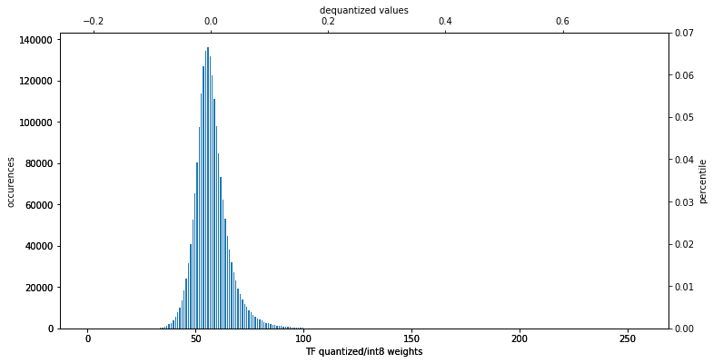
In this work, we assume the quantized filter weights are generated by the uniform affine quantization and represented in unsigned int8 (uint8) together with a dynamic range. Figure 1 illustrates an example of the quantized weights extracted from a fully-connected layer. The bottom x-axis shows the uint8 weights ranging from to ; the top x-axis shows the dequantized fp32 weights.
The spatial filters are transformed into the Winograd domain using the transform matrices. We use in as an example. The filter transform matrix is
which is produced by scaling up the original filter transform matrix Lavin (2015) by a factor of element-wise for integer arithmetic.
Let for , then becomes
Denote the elements in as in the row-major order for a simpler representation, then becomes
In order to adjust for the asymmetry introduced by the uniform affine quantization, the zero-point needs to be subtracted from the uint8 quantized weights, resulting in int9 weights ranging in . As a result, the worst-case magnitudes and bitwidths for each element in are
The same analysis can be applied to the activation transform whose results can be represented by 11-bit. In this paper, we focus on the filter precision scaling that can be preprocessed offline and incur no overhead at inference time.
4.2 Filter Precision Scaling
Targeting quantized filters in the Winograd domain, we propose an efficient lossy precision scaling scheme using only integer arithmetic. We continue to use as the running example.
The precision scaling is applied to the filters used to generate one output feature map (OFM). The scheme computes the minimum downscale factor at each X-Y location across all channels using the maximum magnitude. The scale factors are computed to put the transformed weights back into the int9 range which are then consumed by the multipliers. The downscaled Hadamard products are accumulated over all channels. Finally, the scaling is inverted before the final transforms and .
Since the maximum magnitude in is . The scale factors must cover the range of to . For cost reasons, we implement the scaling by (1) multiplying with a -bit number , and (2) shifting right by a variable amount . That is, the scale factor is in the form of . Recall that transforms a spatial filter to a Winograd-domain filter. Since we share the same scale factor at each X-Y location across all channels, scale factors are computed for a Winograd-domain filter where is the number of channels.
Next we describe the steps to compute the scale factors.
-
1.
Transform all weights for the current OFM.
-
2.
Compute maximum magnitudes for the Winograd-domain kernel.
-
3.
If the maximum magnitude for a given X-Y location , set and to , meaning no scaling applied.
-
4.
Otherwise, set the scale factor to the largest -bit over by
-
(a)
Compute
-
(b)
Compute
-
(c)
-
(d)
.
-
(a)
Note that ranges from to with an offset of , therefore can be represented with bits. As a result, a total of bits are used to specify each scale factor, with the value meaning “no scaling”. The scaling factors are summarized in Table 1 where the out-of-range and some duplicated scale factors are grayed out.
| N | P=0 | P=1 | P=2 | P=3 |
|---|---|---|---|---|
| 1 | 0.06250 | 0.03125 | 0.01563 | 0.00781 |
| 2 | 0.12500 | 0.06250 | 0.03125 | 0.01563 |
| 3 | 0.18750 | 0.09375 | 0.04688 | 0.02344 |
| 4 | 0.25000 | 0.12500 | 0.06250 | 0.03125 |
| 5 | 0.31250 | 0.15625 | 0.07813 | 0.03906 |
| 6 | 0.37500 | 0.18750 | 0.09375 | 0.04688 |
| 7 | 0.43750 | 0.21875 | 0.10938 | 0.05469 |
| 8 | 0.50000 | 0.25000 | 0.12500 | 0.06250 |
| 9 | 0.56250 | 0.28125 | 0.14063 | 0.07031 |
| 10 | 0.62500 | 0.31250 | 0.15625 | 0.07813 |
| 11 | 0.68750 | 0.34375 | 0.17188 | 0.08594 |
| 12 | 0.75000 | 0.37500 | 0.18750 | 0.09375 |
| 13 | 0.81250 | 0.40625 | 0.20313 | 0.10156 |
| 14 | 0.87500 | 0.43750 | 0.21875 | 0.10938 |
| 15 | 0.93750 | 0.46875 | 0.23438 | 0.11719 |
The reverse scaling before the final transforms is applied as a combination of 8-bit multiply and a right shift between 4 and 7 bits, which constitutes to a more precise approximation of the reciprocal of the corresponding scaling factor. During the application of and , note that the original matrix has been scaled up by to , thus a right shift by must be taken after each final transform to cancel the scaling.
4.3 Efficiency and Error Analysis
The transform and downscaling of the filters are performed before inference time, and Winograd-domain filters can be reused during inference. The downscaling step performs comparisons, -bit multiplications, and right shifts, where is the number of weights. The reverse scaling performs only -bit multiplications and right shifts for an entire filter in the Winograd-domain, which reduces the amortized overhead effectively.
Recall that subtracting the zero-point extends the range of quantized weights from uint8 to int9. In the example of , applying the Winograd transforms further extends the required range to 13-bit as calculated in Section 4.1. By using the proposed lossy filter precision scaling scheme, we reduce the range of Winograd weights back to 9-bit, leading to a filter bitwidth reduction of .
The integer approximations of scaling factors introduce errors. We analyze the static errors here and measure the dynamic data-driven errors in terms of inference accuracy loss in Section 4.4.
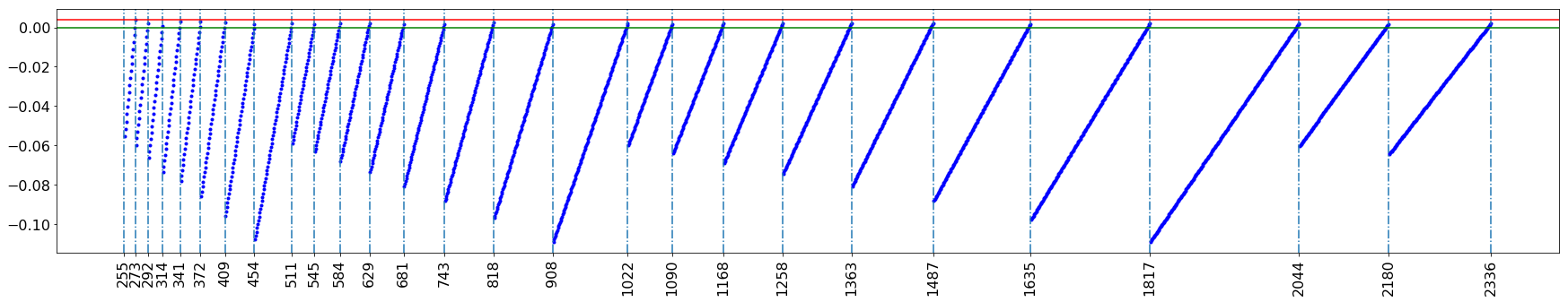
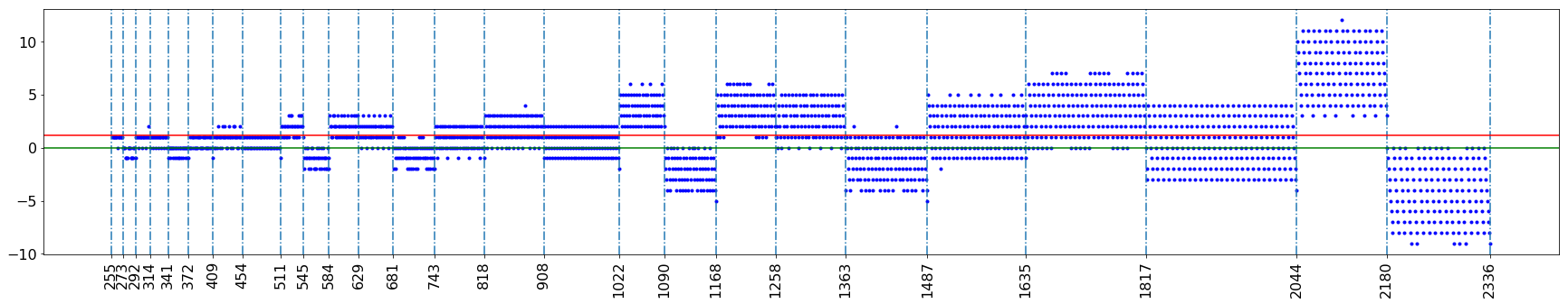
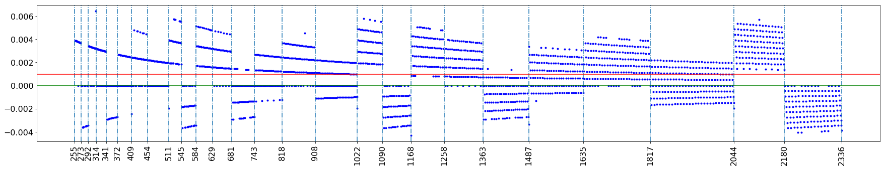
For static scaling errors, Figure 3 uses the dashed vertical lines to show the applicable boundaries and the proportional scaling errors of each unique scaling factor. Figure 4 and 5 describe the numerical and proportional errors of all the scalable weights after being downscaled and then upscaled by the best integer-approximated scaling factors. The average numerical errors is , and the average proportional error is , indicating the filter precision scaling scheme introduces a small positive-biased error overall.
4.4 Evaluation
The filter precision scaling scheme is tested on the combination of popular convnet models of Inception V3 Szegedy et al. (2015) and ResNet V2 50, and a benchmark dataset ILSCVR-12 Russakovsky et al. (2014). To produce the quantized models, we first obtain the pre-trained fp32 models published by TensorFlow-Slim Silberman & Guadarrama (2016). Then we apply the standard quantization approach recommended by TensorFlow TFQ .
The quantization method replaces the fp32 Conv2D nodes in the original pre-trained model with int8 QuantizedConv2D nodes (usually followed by Requantize), an example of which is illustrated by Figure 2 using the TensorBoard TB .
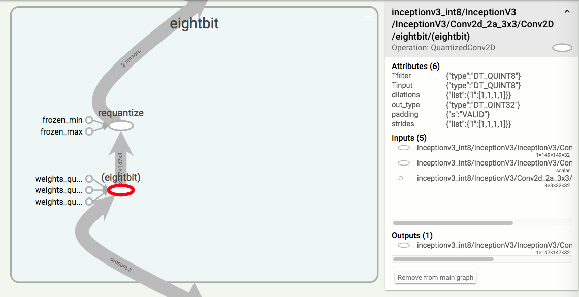
Our experiment captures a subset of QuantizedConv2D nodes in the quantized models where the filter height and width are both and the strides and dilations are both . Note that the nodes with non-unit strides or dilations or of D shapes ( or ) do not affect accuracy and are therefore skipped. The subsets of captured nodes, twelve for Inception V3 and sixteen for ResNet V2 50, are then edited dynamically using the Graph Editor library GE . The editing takes place on two levels:
-
•
On the graph level, the subgraph that contains the captured nodes is duplicated within the same graph, such that the same image will be processed by both the reference subgraph and the Winograd and scaling-enabled counterpart.
-
•
On the node level, each captured QuantizedConv2D node in the duplicated subgraph is replaced with a custom-built convolution scaled by the filter precision scaling method proposed in Section 4.2.
Inception V3. The quantized model records a top-1 accuracy and a top-5 accuracy, the precision-scaled Winograd model achieves a top-1 accuracy and a top-5 accuracy .
ResNet V2 50. The precision-scaled Winograd model leads to a small loss of for top-1 accuracy () and the same top-5 accuracy , compared to the quantized counterpart.
Both experiments confirmed the proposed precision scaling scheme leads to very small accuracy loss for quantized models. Extensive experiments on more neural networks are planned as part of the future work.
5 Conclusion
The Winograd convolution has proved its advantages for the small convolution sizes with the reduction in arithmetic complexity, but also poses challenges to efficient implementation by the emerging kernels and hardware accelerators with integer arithmetic.
This paper is the first to extend the algorithm construction to the field of complex and derive the new complex algorithms for convnets. As an example, the complex achieves a complexity reduction of x over the direct method and an efficiency gain in the range of to over the best-known rational Winograd algorithms with the hardware bitwidth is considered. The derivation method and optimization techniques developed in this paper extend to the construction of larger Winograd convolutions. This paper also answers the challenges from the implementation perspective. We proposed a fast integer-based precision scaling scheme for Winograd-domain filters. The scheme has been analyzed to show a significant reduction in filter bit width with very small static errors. Furthermore, we have shown the combination of Winograd convolution and the lossy scaling scheme can achieve good inference accuracy compared to the reference model without any significant loss.
For future work, a quantitative impact analysis of the additional optimizations listed for complex Winograd convolution will be extended, and more experiments on the impact of precision scaling in a wider range of neural networks will be performed.
Acknowledgements
The authors thank Jens Olson, Andrew Mundy, Rune Holm, Ian Bratt, Eric Kunze and Danny Loh for the insightful discussions and valuable feedback on this paper.
References
- (1) Graph editor (contrib). URL https://www.tensorflow.org/api_guides/python/contrib.graph_editor.
- (2) gemmlowp: a small self-contained low-precision gemm library. URL https://github.com/google/gemmlowp.
- (3) Tensorboard: Graph visualization. URL https://www.tensorflow.org/guide/graph_viz.
- (4) How to quantize neural networks with tensorflow. URL https://www.tensorflow.org/versions/r1.4/performance/quantization.
- Abadi et al. (2016) Abadi, M., Agarwal, A., Barham, P., Brevdo, E., Chen, Z., Citro, C., Corrado, G. S., Davis, A., Dean, J., Devin, M., et al. Tensorflow: Large-scale machine learning on heterogeneous distributed systems. arXiv preprint arXiv:1603.04467, 2016.
- Barabasz et al. (2018) Barabasz, B., Anderson, A., and Gregg, D. Improving accuracy of winograd convolution for dnns. CoRR, abs/1803.10986, 2018.
- Blahut (2010) Blahut, R. Fast Algorithms for Signal Processing. Cambridge University Press, 2010.
- Budden et al. (2016) Budden, D. M., Matveev, A., Santurkar, S., Chaudhuri, S. R., and Shavit, N. Deep tensor convolution on multicores. CoRR, abs/1611.06565, 2016.
- Han et al. (2015) Han, S., Mao, H., and Dally, W. J. Deep compression: Compressing deep neural network with pruning, trained quantization and huffman coding. CoRR, abs/1510.00149, 2015.
- Han et al. (2016) Han, S., Liu, X., Mao, H., Pu, J., Pedram, A., Horowitz, M. A., and Dally, W. J. EIE: efficient inference engine on compressed deep neural network. CoRR, abs/1602.01528, 2016.
- Jia et al. (2018) Jia, Z., Zlateski, A., Durand, F., and Li, K. Optimizing n-dimensional, winograd-based convolution for manycore cpus. SIGPLAN Not., 53(1):109–123, February 2018. ISSN 0362-1340. doi: 10.1145/3200691.3178496.
- Krishnamoorthi (2018) Krishnamoorthi, R. Quantizing deep convolutional networks for efficient inference: A whitepaper. ArXiv e-prints, June 2018.
- Krizhevsky et al. (2012) Krizhevsky, A., Sutskever, I., and Hinton, G. E. Imagenet classification with deep convolutional neural networks. In Proceedings of the 25th International Conference on Neural Information Processing Systems - Volume 1, NIPS’12, pp. 1097–1105, USA, 2012. Curran Associates Inc.
- Lai et al. (2018) Lai, L., Suda, N., and Chandra, V. CMSIS-NN: efficient neural network kernels for arm cortex-m cpus. CoRR, abs/1801.06601, 2018.
- Lavin (2015) Lavin, A. Fast algorithms for convolutional neural networks. CoRR, abs/1509.09308, 2015.
- Li et al. (2017) Li, S. R., Park, J., and Tang, P. T. P. Enabling sparse winograd convolution by native pruning. CoRR, abs/1702.08597, 2017.
- Liu et al. (2018) Liu, X., Pool, J., Han, S., and Dally, W. J. Efficient sparse-winograd convolutional neural networks. CoRR, abs/1802.06367, 2018.
- Mathieu et al. (2013) Mathieu, M., Henaff, M., and LeCun, Y. Fast training of convolutional networks through ffts. CoRR, abs/1312.5851, 2013.
- Migacz (2017) Migacz, S., 2017. URL http://on-demand.gputechconf.com/gtc/2017/presentation/s7310-8-bit-inference-with-tensorrt.pdf.
- (20) Nvidia. Nvidia deep learning accelerator. URL http://http://nvdla.org/.
- Russakovsky et al. (2014) Russakovsky, O., Deng, J., Su, H., Krause, J., Satheesh, S., Ma, S., Huang, Z., Karpathy, A., Khosla, A., Bernstein, M. S., Berg, A. C., and Li, F. Imagenet large scale visual recognition challenge. CoRR, abs/1409.0575, 2014.
- Silberman & Guadarrama (2016) Silberman, N. and Guadarrama, S. Tensorflow-slim image classification model library. 2016. URL https://github.com/tensorflow/models/tree/master/research/slim.
- Sze et al. (2017) Sze, V., Chen, Y., Yang, T., and Emer, J. S. Efficient processing of deep neural networks: A tutorial and survey. CoRR, abs/1703.09039, 2017. URL http://arxiv.org/abs/1703.09039.
- Szegedy et al. (2015) Szegedy, C., Vanhoucke, V., Ioffe, S., Shlens, J., and Wojna, Z. Rethinking the inception architecture for computer vision. CoRR, abs/1512.00567, 2015.
- Vasilache et al. (2014) Vasilache, N., Johnson, J., Mathieu, M., Chintala, S., Piantino, S., and LeCun, Y. Fast convolutional nets with fbfft: A GPU performance evaluation. CoRR, abs/1412.7580, 2014.
- Vincent et al. (2017) Vincent, K., Stephano, K., Michael, F., Boris, G., and Julien, D. On improving the numerical stability of winograd convolutions. 5th International Conference on Learning Representations, 2017.
- Warden (2015) Warden, P. Why are eight bits enough for deep neural networks?, 2015. URL https://petewarden.com/2015/05/23/why-are-eight-bits-enough-for-deep-neural-networks/.
- Warden (2017) Warden, P. Implementing the tensorflow deep learning framework on qualcomm’s low-power dsp, 2017. URL https://www.embedded-vision.com/platinum-members/embedded-vision-alliance/embedded-vision-training/videos/pages/may-2017-embedded-vision-summit-warden.
- Williams et al. (2008) Williams, S., Patterson, D., Oliker, L., Shalf, J., and Yelick, K. The roofline model: A pedagogical tool for program analysis and optimization. In 2008 IEEE Hot Chips 20 Symposium (HCS), pp. 1–71, Aug 2008. doi: 10.1109/HOTCHIPS.2008.7476531.
- Winograd (1980) Winograd, S. Arithmetic Complexity of Computations. CBMS-NSF Regional Conference Series in Applied Mathematics. Society for Industrial and Applied Mathematics, 1980.
- Xygkis et al. (2018) Xygkis, A., Papadopoulos, L., Moloney, D., Soudris, D., and Yous, S. Efficient winograd-based convolution kernel implementation on edge devices. In Proceedings of the 55th Annual Design Automation Conference, DAC ’18, pp. 136:1–136:6, New York, NY, USA, 2018. ACM.
- (32) Zlateski, A., Jia, Z., Li, K., and Durand, F. A deeper look at fft and winograd convolutions.