Optimization of Ride Sharing Systems Using Event-driven Receding Horizon Control^⋆

Abstract

We develop an event-driven Receding Horizon Control (RHC) scheme for a Ride Sharing System (RSS) in a transportation network where vehicles are shared to pick up and drop off passengers so as to minimize a weighted sum of passenger waiting and traveling times. The RSS is modeled as a discrete event system and the event-driven nature of the controller significantly reduces the complexity of the vehicle assignment problem, thus enabling its real-time implementation. Simulation results using actual city maps and real taxi traffic data illustrate the effectiveness of the RH controller in terms of real-time implementation and performance relative to known greedy heuristics.

I Introduction

It has been abundantly documented that the state of transportation systems worldwide is at a critical level. Based on the $2011$ Urban Mobility Report, the cost of commuter delays has risen by $260$% over the past $25$ years and $28$% of U.S. primary energy is now used in transportation [1]. Traffic congestion also leads to an increase in vehicle emissions; in large cities, as much as $90$% of CO emissions are due to mobile sources. Disruptive technologies that aim at dramatically altering the transportation landscape include vehicle connectivity and automation as well as shared personalized transportation through emerging mobility-on-demand systems. Focusing on the latter, the main idea of a Ride Sharing System (RSS) is to assign vehicles in a given fleet so as to serve multiple passengers, thus effectively reducing the total number of vehicles on a road network, hence also congestion, energy consumption, and adverse environmental effects.

The main objectives of a RSS are to minimize the total Vehicle-Miles-Traveled (VMT) over a given time period (equivalently, minimize total travel costs), to minimize the average waiting and traveling times experienced by passengers, and to maximize the number of satisfied RSS participants (both drivers and passengers) [2]. When efficiently managed, a RSS has the potential to reduce the total number of private vehicles in a transportation network, hence also decreasing overall energy consumption and traffic congestion, especially during peak hours of a day. From a passenger standpoint, a RSS is able to offer door-to-door transportation with minimal delays which makes traveling more convenient. From an operator’s standpoint a RSS provides a considerable revenue stream. A RSS also provides an alternative to public transportation or can work in conjunction with it to reduce possible low uitization of vehicles and long passenger delays.

In this paper, we concentrate on designing dynamic vehicle assignment strategies in a RSS aiming to minimize the system-wide waiting and traveling times of passengers. The main challenge in obtaining optimal vehicle assignments is the complexity of the optimization problem involved in conjunction with uncertainties such as random passenger service request times, origins, and destinations, as well as unpredictable traffic conditions which determine the times to pick up and drop off passengers. Algorithms used in RSS are limited by the NP-complete nature of the underlying traveling salesman problem [3] which is a special case of the much more complex problems encountered in RSS optimization. Therefore, a global optimal solution for such problems is generally intractable, even in the absence of the aforementioned uncertainties. Moreover, a critical requirement in such algorithms is a guarantee that they can be implemented in a real-time context.

Several methods have been proposed to solve the RSS problem addressing the waiting and traveling times of passengers. In [4], a greedy approach is used to match vehicles to passenger requests which can on one hand guarantee real-time assignments but, on the other, lacks performance guarantees. The optimization algorithm in [5] improves the average traveling time performance but limits the seat capacity of each vehicle to $2$ (otherwise, the problem becomes intractable for $4$ or more seats) and allows no dynamic allocation of new passengers after a solution is determined. Although vehicles can be dynamically allocated to passengers in [6], all pickup and drop-off events are constrained to take place within a specified time window. The RTV-graph algorithm [7] can also dynamically allocate passengers, but its complexity increases dramatically with the number of agents (passengers and vehicles) and the seat capacity of vehicles. To address the issue of increasing complexity with the size of a RSS, a hierarchical approach is proposed in [3] such that the system is decomposed into smaller regions. Within a region, a mixed-integer linear programs is formulated so as to obtain an optimal vehicle assignment over a sequence of fixed time horizons. Although this method addresses the complexity issue, it involves a large number of unnecessary calculations since there is no need to always re-evaluate an optimal solution over every such horizon. Another approach to reducing complexity, is to abstract a RSS model through passenger and vehicle flows as in [8],[9] and [10]. In [10], for example, the interaction between autonomous mobility-on-demand and public transportation systems is considered so as to maximize the overall social welfare.

In order to deal with the well-known “curse of dimensionality” [11] that characterizes optimization problem formulations for a RSS, we adopt an event-driven Receding Horizon Control (RHC) approach. This is in the same spirit as Model Predictive Control (MPC) techniques [12] with the added feature of exploiting the event-driven nature of the control process in which the RHC algorithm is invoked only when certain events occur. Therefore, compared with conventional time-driven MPC this approach can avoid unnecessary calculations and can significantly improve the efficiency of the RH controller by reacting to random events as they occur in real time. The basic idea of event-driven RHC introduced in [13] and extended in [14] is to solve an optimization problem over a given planning horizon when an event is observed in a way which allows vehicles to cooperate; the resulting control is then executed over a generally shorter action horizon defined by the occurrence of the next event of interest to the controller. Compared to methods such as [5]-[7], the RHC scheme is not constrained by vehicle seating capacities and is specifically designed to dynamically re-allocate passengers to vehicles at any time. Moreover, compared to the time-driven strategy in [3], the event-driven RHC scheme refrains from unnecessary calculations when no event in the RSS occurs. Finally, in contrast to models used in [9] and [10], we maintain control of every vehicle and passenger in a RSS at a microscopic level while ensuring that real-time optimal (over each receding horizon) vehicle assignments can be made.

The paper is organized as follows. We first present in Section II a discrete event system model of a RSS and formulate an optimization problem aimed at minimizing a weighted sum of passenger waiting and traveling times. Section III first reviews the basic RHC scheme previously used and then identifies how it is limited in the context of a RSS. This motivates the new RHC approach described in Section IV, specifically designed for a RSS. Extensive simulation results are given in Section V for actual maps in Ann Arbor, MI and New York City, where, in the latter case, real taxi traffic data are used to drive the simulation model. We conclude the paper in Section VI.

II Problem Formulation

We consider a Ride Sharing System (RSS) in a traffic network consisting of $N$ nodes $\mathcal{N}=\{1,...,N\}$ where each node corresponds to an intersection. Nodes are connected by arcs (i.e., road segments). Thus, we view the traffic network as a directed graph $\mathbb{G}$ which is embedded in a two-dimensional Euclidean space and includes all points contained in every arc, i.e., $\mathbb{G}\subset\mathbb{R}^{2}$. In this model, a node $n\in\mathcal{N}$ is associated with a point $\nu_{n}\in\mathbb{G}$, the actual location of this intersection in the underlying two-dimensional space. The set of vehicles present in the RSS at time $t$ is $\mathcal{A}(t)$, where the index $j\in\mathcal{A}(t)$ will be used to uniquely denote a vehicle, and let $A(t)=|\mathcal{A}(t)|$. The set of passengers is $\mathcal{P}(t)$, where the index $i$ will be used to uniquely denote a passenger, and let $P(t)=|\mathcal{P}(t)|$. Note that $\mathcal{A}(t)$ is time-varying since vehicles may enter or leave the RSS at any time and the same is true for $\mathcal{P}(t)$.

There are two points in $\mathbb{G}$ associated with each passenger $i$, denoted by $o_{i},r_{i}\in\mathbb{G}$: $o_{i}$ is the origin where the passenger issues a service request (pickup point) and $r_{i}$ is the passenger’s destination (drop-off point). Let ${O}(t)=\{o_{1},...,o_{P}\}$ be the set of all passenger origins and ${R}(t)=\{r_{1},...,r_{P}\}$ the corresponding destination set. Vehicles pick up passengers and deliver them to their destinations according to some policy. We assume that the times when vehicles join the RSS are not known in advance, but they become known as a vehicle joins the system. Similarly, the times when passenger service requests occur are random and their destinations become known only upon being picked up.

State Space: In addition to $\mathcal{A}(t)$ and $\mathcal{P}(t)$ describing the state of the RSS, we define the states associated with each vehicle and passenger as follows. Let $x_{j}(t)\in\mathbb{G}$ be the position of vehicle $j$ at time $t$ and let $N_{j}(t)\in\{0,1,...,C_{j}\}$ be the number of passengers in vehicle $j$ at time $t$, where $C_{j}$ is the capacity of vehicle $j$. The state of passenger $i$ is denoted by $s_{i}(t)$ where $s_{i}(t)=0$ if passenger $i$ is waiting to be picked up and $s_{i}(t)=j\in\mathcal{A}(t)$, where $j>0$, when the passenger is in vehicle $j$ after being picked up. Finally, we associate with passenger $i$ a left-continuous clock value $z_{i}(t)\in$ $\mathbb{R}$ whose dynamics are defined as follows: when the passenger joins the system and is added to $\mathcal{P}(t)$, the initial value of $z_{i}(t)$ is $0$ and we set $\dot{z}_{i}(t)=1$, as illustrated in Fig.1 where the passenger service request time is $\varphi_{i}$. Thus, $z_{i}(t)$ may be used to measure the waiting time of passenger $i$. When $i$ is picked up by some vehicle $j$ at time $\rho_{i,j}$ (see Fig.1), $z_{i}(t)$ is reset to zero and thereafter measures the traveling time until the passenger’s destination is reached at time $\sigma_{i,j}$. In summary, the state of the RSS is $\mathbf{X}(t)=\{\mathcal{A}(t),x_{1}(t),\dots,x_{A}(t),N_{1}(t),\dots,N_{A}(t),\mathcal{P}(t),s_{1}(t),\dots,s_{P}(t),\newline z_{1}(t),\dots,z_{P}(t)\}$.

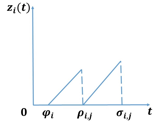
Figure 1: A typical sample path of passenger $i$’s clock state $z_{i}(t)$.

Events: All state transitions in the RSS are event-driven with the exception of the passenger clock states $z_{i}(t)$, $i\in\mathcal{P}(t)$, in which case it is the reset conditions (see Fig.1) that are event-driven. As we will see, all control actions (to be defined) affecting the state $\mathbf{X}(t)$ are taken only when an event takes place. Therefore, regarding a vehicle location $x_{j}(t)$, $j\in\mathcal{A}(t)$, for control purposes we are interested in its value only when events occur, even though we assume that $x_{j}(t)$ is available to the RSS for all $t$ based on an underlying localization system.

We define next the set $E$ of all events whose occurrence causes a state transition. We set $E=E_{U}\cup E_{C}$ to differentiate between uncontrollable events contained in $E_{U}$ and controllable events contained in $E_{C}$. There are six possible event types, defined as follows:

(1) $\alpha_{i}\in E_{U}$: a service request is issued by passenger $i$.

(2) $\beta_{j}\in E_{U}$: vehicle $j$ joins the RSS.

(3) $\gamma_{j}\in E_{U}$: vehicle $j$ leaves the RSS.

(4) $\pi_{i,j}\in E_{C}$: vehicle $j$ picks up passenger $i$ (at $o_{i}\in\mathbb{G}$).

(5) $\delta_{i,j}\in E_{C}$: vehicle $j$ drops off passenger $i$ (at $r_{i}\in\mathbb{G}$).

(6) $\zeta_{m,j}\in E_{C}$: vehicle $j$ arrives at intersection (node) $m\in\mathcal{N}$.

Note that events $\alpha_{i}$, $\beta_{j}$ are uncontrollable exogenous events. Event $\gamma_{j}$ is also uncontrollable, however it may not occur unless the “guard condition” $N_{j}(t)=0$ is satisfied, that is, the number of passengers in vehicle $j$ must be zero when it leaves the system. On the other hand, the remaining three events are controllable. First, $\pi_{i,j}$ depends on the control policy (to be defined) through which a vehicle is assigned to a passenger and is feasible only when $s_{i}(t)=0$ and $N_{j}(t)<C_{j}$. Second, $\delta_{i,j}$ is feasible only when $s_{i}(t)=j\in\mathcal{A}(t)$. Finally, $\zeta_{m,j}$ depends on the policy (to be defined) and occurs when the route taken by vehicle $j$ involves intersection $m\in\mathcal{N}$.

State Dynamics: The events defined above determine the state dynamics as follows.

(1) Event $\alpha_{i}$ adds an element to the passenger set $\mathcal{P}(t)$ and increases its cardinality, i.e., $P(t^{+})=P(t)+1$ where $t$ is the occurrence time of this event. In addition, it initializes the passenger state and associated clock:

$$s_{i}(t^{+})=0,\text{ \ \ }\dot{z}_{i}(t^{+})=1\text{ with }z_{i}(t)=0$$ (1)

and generates the origin information of this passenger $o_{i}\in\mathbb{G}$.

(2) Event $\beta_{j}$ adds an element to the vehicle set $\mathcal{A}(t)$ and increases its cardinality, i.e., $A(t^{+})=A(t)+1$. It also initializes $x_{j}(t)$ to the location of vehicle $j$ at time $t$.

(3) Event $\gamma_{j}$ removes vehicle $j$ from $\mathcal{A}(t)$ and decreases its cardinality, i.e., $A(t^{+})=A(t)-1$.

(4) Event $\pi_{i,j}$ occurs when $x_{j}(t)=o_{i}$ and it generates the destination information of this passenger $r_{i}\in\mathbb{G}$. This event affects the states of both vehicle $j$ and passenger $i$:

$$N_{j}(t^{+})=N_{j}(t)+1,\text{ \ \ }s_{i}(t^{+})=j$$

and, since the passenger was just picked up, the associated clock is reset to $0$ and starts measuring traveling time towards the destination $r_{i}$:

$$z_{i}(t^{+})=0,\text{ \ }\dot{z}_{i}(t^{+})=1$$ (2)

(5) Event $\delta_{i,j}$ occurs when $x_{j}(t)=r_{i}$ and it causes a removal of passenger $i$ from $\mathcal{P}(t)$ and decreases its cardinality, i.e., $P(t^{+})=P(t)-1$. In addition, it affects the state of vehicle $j$:

$$N_{j}(t^{+})=N_{j}(t)-1$$

(6) Event $\zeta_{m,j}$ occurs when $x_{j}(t)=\nu_{m}$. This event triggers a potential change in the control associated with vehicle $j$ as described next.

Control: The control we exert is denoted by $u_{j}(t)\in\mathbb{G}$ and sets the destination of vehicle $j$ in the RSS. We note that the destination $u_{j}(t)$ may change while vehicle $j$ is en route to it based on new information received as various events may take place. The control is initialized when event $\beta_{j}$ occurs at some point $x_{j}(t)$ by setting $u_{j}(t)=\nu_{m}$ where $m\in\mathcal{N}$ is the intersection closest to $x_{j}(t)$ in the direction vehicle $j$ is headed. Subsequently, the vector $\mathbf{u}(t)=\{u_{1}(t),\dots,u_{A}(t)\}$ is updated according to a given policy whenever an event from the set $E$ occurs (we assume that all events are observable by the RSS controller). Our control policy is designed to optimize the objective function described next.

Objective Function: Our objective is to minimize the combined waiting and traveling times of passengers in the RSS over a given finite time interval $[0,T]$. In order to incorporate all passengers who have received service over $[0,T]$, we define the set

$$\mathcal{P}_{T}=\cup_{t\in[0,T]}\mathcal{P}(t)$$

to include all passengers $i\in\mathcal{P}(t)$ for any $t\in[0,T]$. In simple terms, $\mathcal{P}_{T}$ is used to record all passengers who are either currently active in the RSS at $t=T$ or were active and departed at some time $t<T$ when the associated $\delta_{i,j}$ event occurred for some $j\in\mathcal{A}(t)$.

We define $w_{i}$ to be the waiting time of passenger $i$ and note that, according to (1), $w_{i}=z_{i}(t)$ where $t$ is the time when event $\pi_{i,j}$ occurs. Similarly, letting $y_{i}$ be the total traveling time of passenger $i$, according to (2) we have $y_{i}=z_{i}(t)$ where $t$ is the time when event $\delta_{i,j}$ occurs. We then formulate the following problem, given an initial state $\mathbf{X}_{0}$ of the RSS:

$$\min_{\mathbf{u}(t)}E\left[\sum_{i\in\mathcal{P}_{T}}[\mu_{w}w_{i}+\mu_{y}y_{i}]\right]$$ (3)

where $\mu_{w},\mu_{y}$ are weight coefficients defined so that $\mu_{w}=\frac{\omega}{W_{\max}}$ and $\mu_{y}=\frac{1-\omega}{Y_{\max}}$, $\omega\in[0,1]$, and $W_{\max}$ and $Y_{\max}$ are upper bounds of the waiting and traveling time of passengers respectively. The values of $W_{\max}$ and $Y_{\max}$ are selected based on user experience to capture the worst case tolerated for waiting and traveling times respectively. This construction ensures that $w_{i}$ and $y_{i}$ are properly normalized so that (3) is well-defined.

The expectation in (3) is taken over all random event times in the RSS defined in an appropriate underlying probability space. Clearly, modeling the random event processes so as to analytically evaluate this expectation is a difficult task. This motivates viewing the RSS as unfolding over time and adopting a control policy based on observed actual events and on estimated future events that affect the RSS state.

Assuming for the moment that the system is deterministic, let $t_{k}$ denote the occurrence time of the $k$th event over $[0,T]$. A control action $\mathbf{u}(t_{k})$ may be taken at $t_{k}$ and, for simplicity, is henceforth denoted by $\mathbf{u}_{k}$. Along the same lines, we denote the state $\mathbf{X}(t_{k})$ by $\mathbf{X}_{k}$. Letting $K_{T}$ be the number of events observed over $[0,T]$, the optimal value of the objective function when the initial state is $\mathbf{X}_{0}$ is given by

$$J(\mathbf{X}_{0})=\min_{u_{0},\cdots u_{K_{T}}}\left[\sum_{i\in\mathcal{P}_{T}}[\mu_{w}w_{i}+\mu_{y}y_{i}]\right]$$

We convert this into a maximization problem by considering $[-\mu_{w}w_{i}-\mu_{y}y_{i}]$ for each $i\in\mathcal{P}_{T}$. Moreover, observing that both $w_{i}$ and $y_{i}$ are upper-bounded by $T$, we consider the non-negative rewards $T-w_{i}$ and $T-w_{i}$ and rewrite the problem above as

$$J(\mathbf{X}_{0})=\max_{u_{0},\cdots u_{K_{T}}}\left[\sum_{i\in\mathcal{P}_{T}}[\mu_{w}(T-w_{i})+\mu_{y}(T-y_{i})]\right]$$ (4)

Then, determining an optimal policy amounts to solving the following Dynamic Programming (DP) equation [11]:

$$J(\mathbf{X}_{k})=\max_{\mathbf{u}_{k}\in\mathbb{G}}[C(\mathbf{X}_{k},\mathbf{u}_{k})+J_{{k+1}}(\mathbf{X}_{k+1})],\text{ \ }k=0,1,\ldots,K_{T}$$

where $C(\mathbf{X}_{k},\mathbf{u}_{k})$ is the immediate reward at state $\mathbf{X}_{k}$ when control $\mathbf{u}_{k}$ is applied and $J_{{k+1}}(\mathbf{X}_{k+1})$ is the future reward at the next state $\mathbf{X}_{k+1}$. Our ability to solve this equation is limited by the well-known “curse of dimensionality” [11] even if our assumption that the RSS is fully deterministic were to be valid. This further motivates adopting a Receding Horizon Control (RHC) approach as in similar problems encountered in [13] and [14]. This is in the same spirit as Model Predictive Control (MPC) techniques [12] with the added feature of exploiting the event-driven nature of the control process. In particular, in the event-driven RHC approach, a control action taken when the $k$th event is observed is selected to maximize an immediate reward defined over a planning horizon $H_{k}$, denoted by $C(\mathbf{X}_{k},\mathbf{u}_{k},H_{k})$, followed by an estimated future reward $\hat{J}_{{k+1}}(\mathbf{X(}t_{k}+H_{k}))$ when the state is $\mathbf{X(}t_{k}+H_{k})$. The optimal control action $\mathbf{u}_{k}^{\ast}$ is, therefore,

$$\mathbf{u}_{k}^{\ast}=\arg\max_{\mathbf{u}_{k}\in\mathbb{G}}[C(\mathbf{X}_{k},\mathbf{u}_{k},H_{k})+\hat{J}_{{k+1}}(\mathbf{X(}t_{k}+H_{k}))]$$ (5)

The control action $\mathbf{u}_{k}^{\ast}$ is subsequently executed only over a generally shorter action horizon $h_{k}\leq H_{k}$ so that $t_{k+1}=t_{k}+h_{k}$ (see Fig.2). The selection of $H_{k}$ and $h_{k}$ will be discussed in the next section.

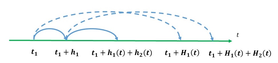
Figure 2: Event-Driven receding horizon control.

III Receding Horizon Control (RHC)

In this section, we first review the basic RHC scheme as introduced in [13], and a modified version in [14] intended to overcome some of the original scheme’s limitations. We refer to the RHC in [13] as RHC1 and the RHC in [14] as RHC2.

The basic RHC scheme in [13] considers a set of cooperating “agents” and a set of “targets” in a Euclidean space. The purpose of agents is to visit targets and collect a certain time-varying reward associated with each target. The key steps of the scheme are as follows: (1) Determine a planning horizon $H_{k}$ at the current time $t_{k}$. (2) Solve an optimization problem to minimize an objective function defined over the time interval $[t_{k},t_{k}+H_{k}]$. (3) Determine an action horizon $h_{k}$ and execute the optimal solution over $[t_{k},t_{k}+h_{k}]$. (4) Set $t_{k+1}=t_{k}+h_{k}$ and return to step (1).

Letting $\mathcal{A}(t)$ be the agent set and $\mathcal{P}(t)$ the target set, we define $d_{i,j}(t)$ for any $i\in\mathcal{P}(t)$, $j\in\mathcal{A}(t)$ to be the distance between target $i$ and agent $j$ at time $t$. In [13], the planning horizon $H_{k}$ is defined as the earliest time that any agent can visit any target in the system:

$$H_{k}=\min_{i\in\mathcal{P}(t),j\in\mathcal{A}(t)}\left\{\dfrac{d_{i,j}(t_{k})}{v}\right\}$$ (6)

where $v$ is the fixed speed of agents. The action horizon $h_{k}$ is defined to be the earliest time in $[t_{k},t_{k}+H_{k}]$ when an event in the system occurs (e.g., a new target appears). In some cases, $h_{k}$ is alternatively defined through $h_{k}=\epsilon H_{k}$ for some $\epsilon\in(0,1]$ so as to ensure that $h_{k}\leq H_{k}$.

In order to formulate the optimization problem to be solved at every control action point $t_{k}$, the concept of neighborhood for a target is defined in [13] as follows. The $k$th nearest agent neighbor to target $l$ is

$$\beta^{k}(l,t)=\underset{i\in\mathcal{A}(t),i\neq\beta_{l}^{1}(t),\dots,i\neq\beta_{l}^{k-1}(t)}{\operatorname{arg}\,\operatorname{min}}\;{d_{l,i}(t)}$$

where $k=1,2,\ldots$, and the $b$-neighborhood of the target is given by the set of the $b$ closest neighbors to it:

$$B_{l}^{b}(t)=\{\beta^{1}(l,t),\dots,\beta^{b}(l,t)\}$$ (7)

Based on (7), for any given $b\geq 1$ the relative distance between agent $i$ and target $l$ is defined as

$$\bar{d}_{l,i}(t)=\left\{\begin{array}[c]{l}\dfrac{d_{l.i}(t)}{\sum_{q\in B_{l}^{b}(t)}d_{l,q}(t)}\\ 1\end{array}\right.\begin{array}[c]{l}\text{if }i\in B_{l}^{b}(t)\\ \text{otherwise}\end{array}$$ (8)

Then, the relative responsibility function of agent $i$ for target $l$ is defined as:

$$p(\bar{d}_{l,i}(t))=\left\{\begin{array}[c]{l}1\\ \dfrac{1-\Gamma-\bar{d}_{l,i}}{1-2\Gamma}\\ 0\end{array}\right.\begin{array}[c]{l}\text{if }\bar{d}_{l,i}\leq\Gamma\\ \text{if }\Gamma\leq\bar{d}_{l,i}\leq 1-\Gamma\\ \text{otherwise}\end{array}$$ (9)

where $p(\bar{d}_{l,i}(t))$ can be viewed as the probability that agent $i$ is the one to visit target $l$. In particular, when the relative distance is small, then $i$ is committed to visit $l$, whereas if the relative distance is large, then $i$ takes no responsibility for $l$. All other cases define a “cooperative region” where agent $i$ visits $l$ with some probability dependent on the parameter $\Gamma$ which is selected so that $\Gamma\in[0,\frac{1}{2})$ and reflects a desired level of cooperation among agents; this cooperation level increases as $\Gamma$ decreases.

The use of $p(\bar{d}_{l,i}(t))$ allows the RHC to avoid early commitments of agents to target visits, since changes in the system state may provide a better opportunity for an agent to improve the overall system performance. A typical example arises when agent $i$ is committed to target $l$ and a new target, say $l^{\prime}$, appears which is in close proximity to $i$; in such a case, it may be beneficial for $i$ to visit $l^{\prime}$ and let $l$ become the responsibility of another agent that may be relatively close to $l$ and uncommitted. This is possible if $p(\bar{d}_{l,i}(t))<1$. In what follows, we will generalize the definition of distance $d_{i,j}(t)$ between target $i$ and agent $j$ to the distance between any two points $x,y\in\mathbb{R}^{2}$ expressed as ${d(x,y)}$.

Using the relative responsibility function, the optimization problem solved by the RHC at each control action point assigns an agent to a point which minimizes a given objective function and which is not necessarily a target point. Details of how this problem is set up and solved and the properties of the RHC1 scheme may be found in [13].

Limitations of RHC1: There are three main limitations of the original RHC scheme:

(1) Agent trajectory instabilities: A key benefit of RHC1 is the fact that early commitments of agents to targets are avoided. As already described above, if a new target appears in the system, an agent en route to a different target may change its trajectory to visit the new one if this is deemed beneficial to the cooperative system as a whole. This benefit, however, is also a cause of potential instabilities when agents frequently modify their trajectories, thus potentially wasting time. It is also possible that an agent may oscillate between two targets and never visit either one. In [13], necessary and sufficient conditions were provided for some simple cases to quantify such instabilities, but these conditions may not always be satisfied.

(2) Future cost estimation inaccuracies: The effectiveness of RHC1 rests on the accuracy of the future cost estimation term $\hat{J}_{{k+1}}(\mathbf{X(}t_{k}+H_{k})$ in (5). In [13], this future cost is estimated through its lower bound, thus resulting in an overly “optimistic” outlook.

(3) Algorithm complexity: In [13], the optimization problem at each algorithm iteration involves the selection of each agent’s heading over $[0,2\pi]$. This is because the planning horizon $H_{k}$ defines a set of feasible reachable points $F_{j}(t_{k},H_{k})=\{w:d(w,x_{j}(t_{k})=vH_{k}\}$ which is a disk of radius $H_{k}/v$ (where $v$ is each agent’s speed) around the agent’s position at time $t_{k}$. This problem must be solved over all agents and incurs considerable computational complexity: if $[0,2\pi]$ is discretized with discretization level $G$, then the complexity of this algorithm at each iteration is $O(G^{A(t)})$.

The modified RCH scheme RHC2 in [14] was developed to address these limitations. To deal with issues (1) and (3) above, a set of active targets $S_{j}(t_{k},H_{k})$ is defined for agent $j$ at each iteration time $t_{k}$. Its purpose is to limit the feasible reachable set $F_{j}(t_{k},H_{k})$ defined by all agent headings over $[0,2\pi]$ so that it is reduced to a finite set of points. Let $x\in F_{j}(t_{k},H_{k})$ be a reachable point and define a travel cost function $\eta_{i}(x,t)$ associated with every target $i\in\mathcal{P}(t)$ measuring the cost of traveling from a point $x$ at time $t$ to a target $i\in\mathcal{P}(t)$. The active target set is defined in [14] as

$$S_{j}(t_{k},H_{k})=\{l:l=\arg\min_{i\in\mathcal{P}(t)}\;\eta_{i}(x,t_{k}+H_{k})$$ (10)

$$\text{ for some }x\in F_{j}(t_{k},H_{k})\}$$

Clearly, $S_{j}(t_{k},H_{k})\subseteq\mathcal{P}(t)$ is a finite set of targets defined by the following property: an active target is closer to some reachable point $x$ than any other target in the sense of minimizing the metric $\eta_{i}(x,t_{k}+H_{k})$. Therefore, if there is some target $l^{\prime}\notin S_{j}(t_{k},H_{k})$, then there is no incentive in considering it as a candidate for agent $j$ to head towards. Restricting the feasible headings of an agent to its active target set not only reduces the complexity of optimally selecting a heading at $t_{k}$, but it also limits oscillatory trajectory behavior, since by (6) there is always an active target on the set $F_{j}(t_{k},H_{k})$ so that eventually all targets are guaranteed to be visited.

Let $\mathbf{u}_{k}$ be the control applied at time $t_{k}$ under planning horizon $H_{k}$. The $j$th component of $\mathbf{u}_{k}$ is the control $u_{j}(t_{k})$ applied to agent $j$, where $u_{j}(t_{k})\in S_{j}(t_{k},H_{k})$ as defined in (10). The estimated time for agent $j$ to reach a target $u_{j}(t_{k})$ is denoted by $\hat{\tau}_{u,j}(\mathbf{u}_{k},t_{k},H_{k})$ where (for notational simplicity) we set $u_{j}(t_{k})=u$. This time is given by

$$\hat{\tau}_{u,j}(\mathbf{u}_{k},t_{k},H_{k})=t_{k}+H_{k}+\frac{1}{v}d(x_{j}(t_{k}),x_{u}),\text{ \ \ }u\in S_{j}(t_{k},H_{k})$$ (11)

where $x_{u}$ is the location of target $u=u_{j}(t_{k})$.

To address issue (2) regarding future cost estimation inaccuracies, a new estimation framework is introduced in [14] by defining a set of targets $\mathcal{T}_{k,j}\subseteq\mathcal{P}(t)-\{u\}$ that agent $j$ would visit in the future, i.e., at $t>t_{k}+H_{k}$, as follows:

$$\mathcal{T}_{k,j}=\{l:p(\bar{d}_{l,j}(t_{k}))>p(\bar{d}_{l,q}(t_{k})),\text{ }\forall q\in\mathcal{A}(t)\}$$ (12)

This set limits the targets considered by agent $j$ to those with a current relative responsibility value in (9) which exceeds that of any other agent. The estimated time to reach a target $l\in\mathcal{T}_{k,j}$ under control $\mathbf{u}_{k}$ and planning horizon $H_{k}$ is denoted by $\hat{\tau}_{l,j}(\mathbf{u}_{k},t_{k},H_{k})$. The first target to be visited in $\mathcal{T}_{k,j}$, denoted by $l^{1}$, is the one with the minimal travel cost from target $u\in S_{j}(t_{k},H_{k})$, i.e., $l^{1}=\arg\min_{l\in\mathcal{T}_{k,j}}\{\eta_{l}(x_{u},\hat{\tau}_{u,j}(\mathbf{u}_{k},t_{k},H_{k}))\}$. Then, all subsequent targets in $\mathcal{T}_{k,j}-\{l^{1}\}$ are similarly ordered as $\{l^{2},l^{3},\ldots\}$. Therefore, setting $\mathcal{T}_{k,j}^{n}=\mathcal{T}_{k,j}-\{l^{1},\ldots,l^{n-1}\}$, $n=2,\ldots,|\mathcal{T}_{k,j}|$, we have

$$l^{n+1}=\arg\min_{l\in\mathcal{T}_{k,j}^{n}}\{\eta_{l}(x_{l^{n}},\hat{\tau}_{l^{n},j}(\mathbf{u}_{k},t_{k},H_{k}))\},\text{ \ }n=1,\ldots,|\mathcal{T}_{k,j}|$$

and

$$\hat{\tau}_{l^{n+1},j}(\mathbf{u}_{k},t_{k},H_{k})=\hat{\tau}_{l^{n},j}(\mathbf{u}_{k},t_{k},H_{k})+\frac{1}{v}d(x_{l^{n}},x_{l^{n+1}})$$ (13)

Limitations of the RHC2 with respect to a RSS:

(1) Euclidean vs. Graph topology: Both RHC1 and RHC2 are based on an underlying Euclidean space topology. In a RSS, however, we are interested in a graph-based topology which requires the adoption of a different distance metric.

(2) Future cost estimation inaccuracies: The travel cost metric $\eta_{i}(x,t)$ used in RHC2 assumes that all future targets to be visited at $t>t_{k}+H_{k}$ are independent of each other and that an agent can visit any target. However, in a RSS, each agent $j$ has a capacity limit $C_{j}$. This has two implications: $(i)$ If a vehicle is full, it must first be assigned to a drop-off point before it can visit a new pickup point, and $(ii)$ The number of future pickup points is limited by $C_{j}-N_{j}(t)$, the residual capacity of vehicle $j$.

The fact that there are two types of “targets” in a RSS (pickup points and drop-off points), also induces an interdependence in the rewards associated with target visits. Whereas in [14] a reward is associated with each target visit, in a RSS the rewards are $w_{i}$ and $y_{i}$ where $y_{i}$ can only be collected after $w_{i}$. This necessitates a new definition of the set $\mathcal{T}_{k,j}$ in (12). For example, if $i\in\mathcal{T}_{k,j}$ and vehicle $j$ is full and must drop off a passenger at a remote location, then using (12) would cause vehicle $j$ to first go to the drop-off location and then return to pick up $i$; however, there may be a free vehicle $k$ in the vicinity of $j$’s current location which is obviously a better choice to assign to passenger $i$.

(3) Agent trajectory instabilities: RHC2 does not resolve the possibility of agent trajectory instabilities. Moreover, the nature of such instabilities is different due to the graph topology used in a RSS.

In view of this discussion, we will present in the next section a new RHC scheme specifically designed for a RSS and addressing the issues identified above. We will keep using the term “target” to refer to points $o_{i}$ and $r_{i}$ for all $i\in\mathcal{P}(t)$.

IV The New RHC Scheme

We begin by introducing some variables used in the new RHC scheme as follows.

(1) $d(u,v)$ is defined as the Manhattan distance [15] between two points $u,v\in\mathbb{G}$. This measures the shortest path distance between two points on a directed graph that includes points on an arc of this graph which belong to $\mathbb{G}\subset\mathbb{R}^{2}$.

(2) $\mathcal{R}_{i,j}(t)$ is the set of the $n$ closest pickup locations in the sense of the Manhattan distance defined above, where $n=C_{j}-N_{j}(t)-1$ if $j$ picks up $i$ at $o_{i}$ at time $t$, and $n=C_{j}-N_{j}(t)+1$ if $j$ drops off $i$ at $r_{i}$ at time $t$. Clearly, the set may contain fewer than $n$ elements if there are insufficient pickup locations in the RSS at time $t$.

(3) $\hat{\mathcal{R}}_{i,j}(t)$ is the set of $n$ drop-off locations for $j$, where $n=N_{j}(t)+1$ if $j$ picks up $i$ at $o_{i}$, and $n=N_{j}(t)-1$ if $j$ drops off $i$ at $r_{i}$.

(4) $\varphi_{i}$ and $\rho_{{i,j}}$ denote the occurrence time of events $\alpha_{i}$ (passenger $i$ joins the RSS) and $\pi_{i,j}$ (pickup of passenger $i$ by vehicle $j$) respectively.

In the rest of this section we present the new RHC scheme which overcomes the issues previously discussed through four modifications: $(i)$ We define the travel value of a passenger for each vehicle considering the distance between vehicles and passengers, as well as the vehicle’s residual capacity. $(ii)$ Based on the new travel value and the graph topology of the map, we introduce a new active target set for each vehicle during $[t_{k},t_{k}+H_{k})$. This allows us to reduce the feasible solution set of the optimization problem (5) at each iteration. $(iii)$ We develop an improved future reward estimation mechanism to better predict the time that a passenger is served in the future. $(iv)$ To address the potential instability problem, a method to restrain oscillations is introduced in the optimization algorithm at each iteration.

Each of these modifications is described below, leading to the new RHC scheme. We begin by defining the planning horizon $H_{k}$ at the $k$th control update consistent with (6) as

$$H_{k}=\min_{i\in\mathcal{P}(t_{k}),j\in\mathcal{A}(t_{k})}\left\{\frac{d(x_{j}(t_{k}),c_{i})}{v_{j}(t_{k})}\right\}$$ (14)

where

$$c_{i}=\left\{\begin{array}[c]{l}o_{i}\\ r_{i}\\ \end{array}\right.\begin{array}[c]{l}\text{if }s_{i}(t)=0\text{ and }N_{j}(t_{k})<C_{j}\\ \text{if }s_{i}(t)=j\\ \end{array}$$ (15)

and $v_{j}(t_{k})$ is the maximal speed of vehicle $j$ at time $t_{k}$, assumed to be maintained over $[t_{k},t_{k}+H_{k}]$. Thus, $H_{k}$ is the shortest Manhattan distance from any vehicle location to any target (either $o_{i}$ or $r_{i}$) at time $t_{k}$. Note that $c_{i}$ is undefined if $s_{i}(t)=0$ and $N_{j}(t_{k})=C_{j}$. Formally, to ensure consistency, we set $d(x_{j}(t_{k}),c_{i})=\infty$ if $s_{i}(t)=0$ and $N_{j}(t_{k})=C_{j}$ since $o_{i}$ is not a valid pickup point for $j$ in this case.

The action horizon $h_{k}\leq H_{k}$ is defined by the occurrence of the next event in $E$, i.e., $h_{k}=\tau_{k+1}-t_{k}$ where $\tau_{k+1}$ is the time of the next event to occur after $t_{k}$. If no such event occurs over $[t_{k},t_{k}+H_{k}]$, we set $h_{k}=H_{k}$.

IV-A Vehicle Travel Value Function

Recall that in RHC2 a travel cost function $\eta_{i}(x,t)$ was defined for any agent measuring the cost of traveling from a point $x$ at time $t$ to a target $i\in\mathcal{P}(t)$. In our case, we define instead a travel value measuring the reward (rather than cost) associated with a vehicle $j$ when it considers any passenger $i\in\mathcal{P}(t)$. There are three cases to consider depending on the state $s_{i}(t)$ for any $i\in\mathcal{P}(t)$ as follows:

Case 1: If $s_{i}(t)=0$, then passenger $i$ is waiting to be picked up. From a vehicle $j$’s point of view, there are two components to the value of picking up this passenger at point $o_{i}$: $(i)$ The accumulated waiting time $t-\varphi_{i}$ of passenger $i$; the larger this waiting time, the higher the value of this passenger is. $(ii)$ The distance of $j$ from $o_{i}$; the shorter the distance, the higher the value of this passenger is. To ensure this value component is non-negative, we define $D$ to be the largest possible travel time between any two points in the RSS (often referred to as the diameter of the underlying graph) and consider $D-d(x_{j}(t),o_{i})$ as this value component.

In order to properly normalize each component and ensure its associated value is restricted to the interval $[0,1]$, we use the waiting time upper bound $W_{\max}$ introduced in (3) and the distance upper bound $D$ to define the total travel value function as

$$V_{i,j}(x_{j}(t),t)=(1-\mu)\cdot\dfrac{t-\varphi_{i}}{W_{\max}}+\mu\cdot\frac{D-d(x_{j}(t),o_{i})}{D}$$ (16)

where $\mu\in[0,1]$ is a weight coefficient depending on the relative importance the RSS places on passenger satisfaction (measured by waiting time) and vehicle distance traveled. In the latter case, a large value of $d(x_{j}(t),o_{i})$ implies that vehicle $j$ wastes time either traveling empty (if $N_{j}(t)=0$) or adding to the traveling time of passengers already on board (if $N_{j}(t)>0$).

Case 2: If $s_{i}(t)=j\in\mathcal{A}(t)$, then passenger $i$ is already on board with destination $r_{i}$. From vehicle $j$’s point of view, there are again two components to the value of delivering this passenger to point $r_{i}$: $(i)$ The accumulated travel time $t-\rho_{i,j}$ of passenger $i$. $(ii)$ The distance of $j$ from $r_{i}$. Similar to (16), we define

$$V_{i,j}(x_{j}(t),t)=(1-\mu)\cdot\dfrac{t-\rho_{i,j}}{Y_{\max}}+\mu\cdot\frac{D-d(x_{j}(t),r_{i})}{D}$$ (17)

where $Y_{\max}$ is the travel time upper bound introduced in (3).

Case 3: If $s_{i}(t)=k\neq j$, $k\in\mathcal{A}(t)$, then passenger $i$ is already on board some other vehicle $k\neq j$. Therefore, from vehicle $j$’s point of view, the value of this passenger is $V_{i,j}(x_{j}(t),t)=0$.

We summarize the definition of the travel value function as follows:

$$V_{i,j}(x_{j}(t),t)=\left\{\begin{array}[c]{cc}(1-\mu)\cdot\frac{t-\varphi_{i}}{W_{\max}}+\mu\cdot\frac{D-d(x_{j}(t),o_{i})}{D}&\text{if }s_{i}(t)=0\\ (1-\mu)\cdot\frac{t-\rho_{i,j}}{Y_{\max}}+\mu\cdot\frac{D-d(x_{j}(t),r_{i})}{D}&\text{if }s_{i}(t)=j\\ 0&\text{otherwise}\end{array}\right.$$ (18)

In addition to this “immediate” value associated with passenger $i$, there is a future value for vehicle $j$ to consider depending on the sets $\mathcal{R}_{i,j}(t)$ and $\hat{\mathcal{R}}_{i,j}(t)$ defined earlier. In particular, if $s_{i}(t)=0$ and vehicle $j$ proceeds to the pickup location $o_{i}$, then the value associated with $\mathcal{R}_{i,j}(t)$ is defined as

$$V_{i,j}^{\mathcal{R}}(x_{j}(t),t)=\max_{n\in\mathcal{R}_{i,j}(t)}V_{n,j}(o_{i},t)$$

which is the maximal travel value among all passengers in $\mathcal{R}_{i,j}(t)$ to be collected if vehicle $j$ selects $o_{i}$ as its destination at time $t$. On the other hand, if $s_{i}(t)=j$ and vehicle $j$ proceeds to the drop-off location $r_{i}$, then $V_{n,j}(o_{i},t)$ above is replaced by $V_{n,j}(r_{i},t)$. Since the value of $s_{i}(t)$ is known to $j$, we will use $c_{i}$ as defined in (15) and write

$$V_{i,j}^{\mathcal{R}}(x_{j}(t),t)=\max_{n\in\mathcal{R}_{i,j}(t)}V_{n,j}(c_{i},t)$$

Similarly, the value of $\hat{\mathcal{R}}_{i,j}(t)$ is defined as

$$V_{i,j}^{\hat{\mathcal{R}}}(x_{j}(t),t)=\max_{n\in\hat{\mathcal{R}}_{i,j}(t)}V_{n,j}(c_{i},t)$$

We then define the total travel value associated with a vehicle $j$ when it considers any passenger $i\in\mathcal{P}(t)$ as

$$\bar{V}_{i,j}(x_{j}(t),t)=V_{i,j}(x_{j}(t),t)+\max\{V_{i,j}^{\mathcal{R}}(x_{j}(t),t),V_{i,j}^{\hat{\mathcal{R}}}(x_{j}(t),t)\}$$ (19)

Figure 3 shows an example of how $\bar{V}_{i,j}(x_{j}(t),t)$ is evaluated by vehicle $j$ in the case where $c_{i}=o_{i}$ (i.e., $s_{i}(t)=0$). In this case, $\mathcal{R}_{i,j}(t)=\{k,l,p\}$ and $\hat{\mathcal{R}}_{i,j}(t)=\{m,n\}$.

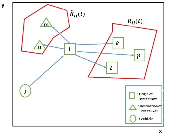
Figure 3: Travel value of passenger $i$ evaluated by vehicle $j$ when $s_{i}(t)=0$.

IV-B Active Target Sets

The concept of an active target set was introduced in [14]. Clearly, this cannot be used in a RSS since the topology is no longer Euclidean and the travel cost function $\eta_{i}(x,t)$ has been replaced by the travel value function (19).

We begin by defining the reachability (or feasible) set $F_{j}(t_{k},H_{k})$ for vehicle $j$ in the RSS topology specified by $\mathbb{G}\subset\mathbb{R}^{2}$. This is now a finite set consisting of horizon points in $\mathbb{G}$ reachable through some path starting from $x_{j}(t_{k})$ and assuming a fixed speed $v_{j}(t_{k})$ as defined in (14). This is illustrated in Fig. 4 where $F_{j}(t_{k},H_{k})$ consists of 10 horizon points (one-way streets have been taken into account as directed arcs in the underlying graph). Observe that $H_{k}$ in this example is defined by $o_{2}$, the pickup location of passenger 2 (horizon point $5$) in accordance with (14). Note that since the actual speed of the vehicle may be lower than $v_{j}(t_{k})$, it is possible that no horizon point is reached at time $t_{k}+h_{k}$ even if $h_{k}=H_{k}$. This simply implies that a new planning horizon $H_{k+1}$ is evaluated at $t_{k}+H_{k}$ (which might still be defined by $o_{2}$).

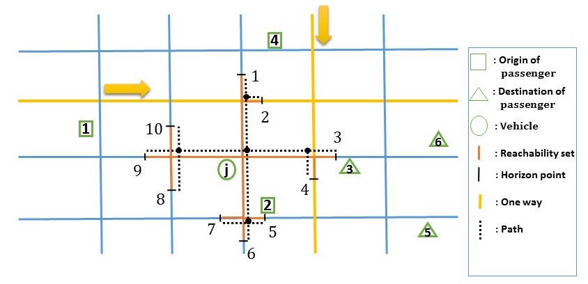
Figure 4: Example of the reachability set of vehicle $j$.

We can now define the active target set of vehicle $j$ to consist of any target (pickup or drop-off locations of passengers) which has the largest travel value to $j$ for at least one horizon point $x\in F_{j}(t_{k},H_{k})$.

Definition: The set of Active Targets of vehicle $j$ is defined as

$$S_{j}(t_{k},H_{k})=\{l:l=\arg\max_{i\in\mathcal{P}(t)}\;\bar{V}_{i,j}(x,t_{k}+H_{k})$$ (20)

$$\text{ for some }x\in F_{j}(t_{k},H_{k})\}$$

Observe that $S_{j}(t_{k},H_{k})\subseteq\mathcal{P}(t_{k})$ and may reduce the number of passengers to consider as potential destinations assigned to $j$ when $S_{j}(t_{k},H_{k})\subset\mathcal{P}(t_{k})$ since

$$u_{j}(t_{k})\in S_{j}(t_{k},H_{k})$$

In the example of Fig. 4, $\mathcal{P}(t_{k})$ contains 6 passengers where $s_{1}(t_{k})=s_{2}(t_{k})=s_{4}(t_{k})=0$ and $s_{3}(t_{k})=s_{5}(t_{k})=s_{6}(t_{k})=j$. Thus, we can immediately see that $P(t_{k})=6<$ $\left|F_{j}(t_{k},H_{k})\right|=10$. Further, observe that the drop-off points $r_{5}$ and $r_{6}$ are such that $r_{5},r_{6}\notin S_{j}(t_{k},H_{k})$ since both points are farther away from $x_{j}(t_{k})$ than $r_{3}$ and $o_{2}$ respectively. Therefore, the optimal control selection to be considered at $t_{k}$ is reduced to $u_{j}(t_{k})\in S_{j}(t_{k},H_{k})=\{o_{1},o_{2},r_{3},o_{4}\}$. In addition, if the capacity $C_{j}$ happens to be such that $C_{j}=3$, then the only feasible control would be $u_{j}(t_{k})=r_{3}$.

IV-C Future Reward Estimation

In order to solve the optimization problem (5) at each RHC iteration time $t_{k}$, we need to estimate the time that a future target is visited when $t>t_{k}+H_{k}$ so as to evaluate the term $\hat{J}_{{k+1}}(\mathbf{X(}t_{k}+H_{k}))$. Let us start by specifying the immediate reward term $C(\mathbf{X}_{k},\mathbf{u}_{k},H_{k})$ in (5). In view of (4), there are three cases: $(i)$ As a result of $\mathbf{u}_{k}$, an event $\pi_{i,j}$ (where $s_{i}(t)=j$) occurs at time $t_{k+1}$ with an associated reward $C(\mathbf{X}_{k},\mathbf{u}_{k},H_{k})=\mu_{w}(T-w_{i})$ where $w_{i}=t_{k+1}-\varphi_{i}$, $(ii)$ As a result of $\mathbf{u}_{k}$, an event $\delta_{i,j}$ occurs at time $t_{k+1}$ with an associated reward $C(\mathbf{X}_{k},\mathbf{u}_{k},H_{k})=\mu_{y}(T-y_{i})$ where $y_{i}=t_{k+1}-\rho_{{i,j}}$, and $(iii)$ Any other event results in no immediate reward. In summary, adopting the notation $C(\mathbf{u}_{k},t_{k+1})$ for the immediate reward resulting from control $\mathbf{u}_{k}$, we have

$$C(\mathbf{u}_{k},t_{k+1})=\left\{\begin{array}[c]{cc}\mu_{w}(T-w_{i})&\text{if event }\pi_{i,j}\text{ occurs at }t_{k+1}\\ \mu_{y}(T-y_{i})&\text{if event }\delta_{i,j}\text{ occurs at }t_{k+1}\\ 0&\text{otherwise}\end{array}\right.$$ (21)

In order to estimate future rewards at times $t>t_{k+1}$, recall that $\mathcal{T}_{k,j}\subseteq\mathcal{P}(t)-\{u_{j}(t_{k})\}$ is a set of targets that vehicle $j$ would visit in the future, after reaching $u_{j}(t_{k})$. This set was defined in [14] through (12) and a new definition suitable for the RSS will be given below. Then, for each target $n\in\mathcal{T}_{k,j}$ the associated reward is $C(\mathbf{u}_{k},\hat{\tau}_{n,j})$ where $\hat{\tau}_{n,j}$ is the estimated time that vehicle $j$ reaches target $n$. If $n=o_{i}$ for some passenger $i$, then, from (21), $C(\mathbf{u}_{k},\hat{\tau}_{n,j})=\mu_{w}(T-\hat{w}_{i})$ where $\hat{w}_{i}=\hat{\tau}_{n,j}-\varphi_{i}$, whereas if $n=r_{i}$ for some passenger $i$, then $C(\mathbf{u}_{k},\hat{\tau}_{n,j})=\mu_{y}(T-\hat{y}_{i})$ where $\hat{y}_{i}=\hat{\tau}_{n,j}-\rho_{{i,j}}$. Further, we include a discount factor $\lambda_{n}(\hat{\tau}_{n,j})$ to account for the fact that the accuracy of our estimate $\hat{\tau}_{n,j}$ is monotonically decreasing with time, hence $\lambda_{n}(\hat{\tau}_{n,j})\in(0,1]$. Therefore, for each vehicle $j$ the associated term for $\hat{J}_{{k+1}}(\mathbf{X(}t_{k}+H_{k}))$ is

$$\hat{J}_{j}(\mathbf{X}(t_{k}+H_{k}))=\sum_{n=1}^{\left|\mathcal{T}_{k,j}\right|}\lambda_{n}(\hat{\tau}_{n,j})C(u_{k,j},\hat{\tau}_{n,j})$$ (22)

and

$$\hat{J}(\mathbf{X}(t_{k}+H_{k}))=\sum_{j\in\mathcal{A}(t_{k})}\hat{J}_{j}(\mathbf{X}(t_{k}+H_{k}))$$ (23)

We now need to derive estimates $\hat{\tau}_{n,j}$ for each $n\in\mathcal{T}_{k,j}$. These estimates clearly depend on the order imposed on the elements of $\mathcal{T}_{k,j}$, i.e., the expected order that vehicle $j$ follows in reaching the targets (after it reaches $u_{j}(t_{k})$) contained in this set. As already explained under (2) at the end of the last section, this order depends on the passenger states and the residual capacity of the vehicle. Suppose that the order is specified through $\theta_{n}^{j}$ defined as the $n$th target label in $\mathcal{T}_{k,j}$ (e.g., $\theta_{1}^{j}=4$ indicates that target $4$ is the first to be visited). Then, (22) is rewritten as

$$\hat{J}_{j}(\mathbf{X}(t_{k}+H_{k}))=\sum_{n=1}^{\left|\mathcal{T}_{k,j}\right|}\lambda_{\theta_{n}^{j}}(\hat{\tau}_{\theta_{n}^{j},j})C(u_{k,j},\hat{\tau}_{\theta_{n}^{j},j})$$ (24)

It now remains to $(i)$ define the set $\mathcal{T}_{k,j}$, suitably modified from (12) to apply to a RSS, so as to address the inaccuracy limitation (2) described at the end of the last section, and $(ii)$ Specify the ordering $\{\theta_{1}^{j},\ldots,\theta_{\left|\mathcal{T}_{k,j}\right|}^{j}\}$ imposed on the elements of $\mathcal{T}_{k,j}$.

We proceed by defining target subsets of $\mathcal{T}_{k,j}$ ordered in terms of the priority of vehicle $j$ to visit these targets compared to other vehicles. This is done using the relative responsibility function in (9) with the Manhattan distance used in evaluating $\bar{d}_{l,i}(t)$. Thus, let $\mathcal{T}_{k,j}=\mathcal{T}_{k,j}^{1}\cup\dots\cup\mathcal{T}_{k,j}^{M}$ where $\mathcal{T}_{k,j}^{m}$ has the $m$th highest priority among all subsets and $M\leq P(t)$ is the number of subsets. When $m=1$, we have

$$\mathcal{T}_{k,j}^{1}=\{l:p(\bar{d}_{l,j}(t_{k}))>p(\bar{d}_{l,q}(t_{k})),\text{ }\forall q\in\mathcal{A}(t),\text{ \ }\forall l\in\mathcal{P}(t)\}$$

which is the same as (12): this is the passenger “responsibility set” of vehicle $j$ in the sense that this vehicle has a higher responsibility value in (9) for each passenger in $\mathcal{T}_{k,j}^{1}$ than that of any other vehicle. Note that if $s_{l}(t_{k})=j$, then by default we have $l\in T_{k,j}^{1}$ since the drop-off location $r_{i}$ is the exclusive responsibility of vehicle $j$. For passengers with $s_{l}(t_{k})=0$, they are included in $T_{k,j}^{1}$ as long as there is no other vehicle $q\neq j$ with a higher relative responsibility for $l$ than that of $j$.

Next, let $\mathcal{A}_{l,m}(t)$ be a subset of vehicles defined as

$$\mathcal{A}_{l,m}(t_{k})=\{j:l\notin\mathcal{T}_{k,j}^{n},\text{ }n<m,\text{ \ }j\in\mathcal{A}(t_{k})\}$$

This subset contains all vehicles which do not have target $l$ included in any of their top $m-1$ priority subsets. We then define $\mathcal{T}_{k,j}^{m}$ when $m>1$ as follows:

$$\mathcal{T}_{k,j}^{m}=\{l:p(\bar{d}_{l,j}(t_{k}))>p(\bar{d}_{l,q}(t_{k})),\text{ }\forall q\in\mathcal{A}_{l,m}(t_{k}),$$ (25)

$$\text{ }\forall l\notin\mathcal{T}_{k,j}^{n},n<m\text{\ }\}$$

This set contains all targets for which $j$ has a higher relative responsibility than any other vehicle and which have not been included in any higher priority set $\mathcal{T}_{k,j}^{n},$ $n<m$. As an example, suppose passenger $i$ is waiting to be picked up and belongs to $T_{k,j_{1}}^{1}$, $T_{k,j_{2}}^{2}$ and $T_{k,j_{3}}^{3}$, where $j_{1}$ is the closest vehicle to $i$. Suppose vehicle $j_{1}$ is full and needs to drop off a passenger first whose destination is far away. Because vehicle $j_{2}$ has the $2$nd highest priority, then $j_{2}$ may serve $i$ provided it has available seating capacity. If $j_{2}$ cannot serve $i$, then vehicle $j_{3}$ with a lower priority is the next to consider serving $i$. In this manner, we overcome the limitation of (12) where no agent capacity is taken into account.

The last step is to specify the ordering $\{\theta_{1}^{j},\ldots,\theta_{\left|T_{k,j}^{m}\right|}^{j}\}$ imposed on each set $T_{k,j}^{m},$ $j\in\mathcal{A}(t)$, $m=1,\ldots,M$. This is accomplished by using the travel value function $\bar{V}_{i,j}(x_{j}(t),t)$ in (19) as follows:

$$\bar{V}_{\theta_{n+1}^{j},j}(c_{\theta_{n}^{j}},\hat{\tau}_{\theta_{n}^{j},j}) \leq\bar{V}_{i,j}(c_{\theta_{n}^{j}},\hat{\tau}_{\theta_{n}^{j},j})$$ (26)

$$\text{for all }i \in T_{k,j}^{m}-\{\theta_{1}^{j},\dots,\theta_{n}^{j}\}$$

where we have used the definition of $c_{i}$ in (15). Setting $u=u_{j}(t_{k})$, the estimated times are given by

$$\hat{\tau}_{\theta_{1}^{j},j} =t_{k}+\frac{1}{v}d(x_{j}(t_{k}),x_{u})+\frac{1}{v}d(u,c_{\theta_{1}^{j},j})$$ (27)

$$\hat{\tau}_{\theta_{n}^{j},j} =\hat{\tau}_{\theta_{n-1}^{j},j}+\frac{1}{v}d(c_{\theta_{n-1}^{j},j},c_{\theta_{n}^{j},j}),\text{ \ }n>1$$ (28)

where $\hat{\tau}_{\theta_{1}^{j},j}$ is the estimated time of reaching the target with the highest travel value beyond the one selected as $u_{j}(t_{k})$ among all targets in $T_{k,j}^{m}$ and $\hat{\tau}_{\theta_{n}^{j},j}$ for $n>1$ is the estimated time of reaching the $n$th target in the order established through (26). Note that this approach takes into account the state of vehicle $j$; in particular, if $N_{j}(t)=C_{j}$, then the ordering of targets in $T_{k,j}^{m}$ is limited to those such that $s_{i}(t_{k})=j$.

This completes the evaluation of the estimated future reward in (23) based on (21) and (22), along with the ordering of future targets specified through (26).

IV-D Preventing Vehicle Trajectory Instabilities

Our final concern is the issue of instabilities discussed under (3) at the end of the last section. This problem arises when a new passenger joins the system and introduces a new target for one or more vehicles in its vicinity which may have higher travel value in the sense of (19) than current ones. As a result, a vehicle may switch its current destination $u_{j}(t_{k})$ and this process may repeat itself with additional future new passengers. In order to avoid frequent such switches, we introduce a threshold parameter denoted by $\Theta$ and react to any event $\alpha_{i}$ (a service request issued by a new passenger $i$) that occurs at time $t_{k}$ as follows:

$$u_{j}(t_{k})=\left\{\begin{array}[c]{cc}o_{i}&\begin{array}[c]{c}\text{if }\bar{V}_{i,j}(x_{j}(t_{k}),o_{i})-\bar{V}_{u,j}(x_{j}(t_{k}),x_{u})>\Theta\text{,}\\ N_{j}(t)<C_{j}\text{, }j=1,\ldots,A(t_{k})\end{array}\\ u&\text{otherwise}\end{array}\right.$$ (29)

where $u=u_{j}(t_{k-1})$ is the current destination of $j$. In simple terms, the current control remains unaffected unless the new passenger provides an incremental value relative to this control which exceeds a given threshold. Since (29) is applied to all vehicles in the current vehicle set $\mathcal{A}(t)$, the vehicle with the largest incremental travel value ends up with $o_{i}$ as its control as long as it exceeds $\Theta$. Note that the new passenger may not be assigned to $j$ unless this vehicle has a positive residual capacity.

IV-E RHC optimization scheme

The RHC scheme consists of a sequence of optimization problems solved at each event time $t_{k}$, $k=1,2,\ldots$with each problem of the form

$$\mathbf{u}_{k}^{\ast}= \arg\max_{\begin{subarray}{c}u_{k,j}\in S_{j}(t_{k},H_{k})\\ j\in\mathcal{A}(t_{k})\end{subarray}}[C(\mathbf{u}_{k},t_{k+1})$$ (30)

$$+\sum_{j\in\mathcal{A}(t_{k})}\sum_{n=1}^{\left|T_{k,j}^{m}\right|}\lambda_{\theta_{n}^{j}}(\hat{\tau}_{\theta_{n}^{j},j})C(u_{k,j},\hat{\tau}_{\theta_{n}^{j},j})]\text{, \ }m=1,\ldots,M$$

where $S_{j}(t_{k},H_{k})$ is the active target of vehicle $j$ at time $t_{k}$ obtained through (20), $C(\mathbf{u}_{k},t_{k+1})$ is given by (21), and $\hat{\tau}_{\theta_{n}^{j},j}$ is evaluated through (27)-(28) with the ordering $\{\theta_{1}^{j},\ldots,\theta_{\left|T_{k,j}^{m}\right|}^{j}\}$ given by (26) and the sets $\mathcal{T}_{k,j}^{m}$, $m=1,\ldots,M$, defined through (25). Note that (30) must be augmented to include (29) when the event occurring at $t_{k}$ is of type $\alpha_{i}$.

An algorithmic description of the RHC scheme is given in Algorithm $1$

1) Determine $H_{k}$ through (14);

2) Determine the active target set $S_{j}(t_{k},H_{k})$ through (20) for all $j\in\mathcal{A}(t)$;

3) Evaluate the estimated future reward through (27) and (28) for all candidate optimal controls;

4) Determine the optimal control $\mathbf{u^{*}_{k}}$ in (30);

5) Execute $\mathbf{u^{*}_{k}}$ until an event occurs;

if a new passenger $i$ enters the system then

      

      for each vehicle $j$ with $N_{j}(t)<C_{j}$ do

             calculate $\bar{V}_{i,j}(x_{j}(t_{k}),o_{i})$;

             if  $\bar{V}_{i,j}(x_{j}(t_{k}),o_{i})-\bar{V}_{u,j}(x_{j}(t_{k}),x_{u})>\Theta$ then

                   we set $i$ as the new target;

                   break;

                  

             end if

            

       end for

      

end if

Algorithm 1 RHC Algorithm.

Complexity of Algorithm $1$: The complexity of the original RHC in [13] was discussed in Section III. For the new RHC we have developed, the optimal control for vehicle $j$ at any iteration is selected from the finite set $S_{j}(t_{k},H_{k})$ defined by active targets. Thus, the complexity is $O(\Omega^{A(t)})$ where $\Omega\leq P(t)$ (the number of targets) is the maximum number of active targets. Observe that $\Omega$ decreases as targets are visited if new ones are not generated.

V Simulation Results

We use the SUMO (Simulation of Urban Mobility) [16] transportation system simulator to evaluate our RHC for a RSS applied to two traffic networks (in Ann Arbor, MI and in New York City, NY). Among other convenient features, SUMO may be employed to simulate large-scale traffic networks and to use traffic data and maps from other sources, such as OpenStreetMap and VISUM. Vehicle speeds are set by the simulation and they include random factors like different road speed limits, turns, traffic lights, etc.

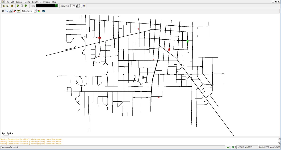
Figure 5: A RSS in the Ann Arbor map.

V-A RHC for a RSS in the Ann Arbor map

A RSS for part of the Ann Arbor map is shown in Fig.5. Green colored vehicles are idle while red colored ones contain passengers to be served. A triangle along a road indicates a waiting passenger. We pre-load in SUMO a fixed number of vehicles, while passengers request service at random points in time as the simulation runs. Passenger arrivals are modeled as a Poisson process with a rate of $3$ passengers/min. The remaining RSS system parameters are selected as follows: $C_{j}=4$, $T=300$ min, $W_{max}=47$ min, $Y_{max}=47$ min, $D=3000$ m and the threshold in (29) is set at $\Theta=0.3$.

Figure 6: Waiting and traveling time histograms under different weights $\omega$ for the Ann Arbor RSS.

In Table I, the average waiting and traveling times under RHC are shown for different weights $\omega$ in the Ann Arbor RSS. The results are averaged over three independent simulation runs. In this example, the number of pre-loaded vehicles is $7$ and simulations end after $30$ passengers are delivered to associated destinations (which is within T=300 min set above). In order to evaluate the performance of the RSS at steady state, we allow a simulation to “warm up” before starting to measure the $30$ passengers served over the course of a simulation run.

The first column of Table I shows different values of the weights $\omega$ as defined in (3) specifying the relative importance assigned to passenger waiting and traveling respectively. As expected, emphasizing waiting results in larger vehicle occupancy and longer average travel times. In Fig. 6 we provide the waiting and traveling time histograms for all cases in Table I.

In Table II, we compare our RHC method with a greedy heuristic (GH) algorithm (similar to [4]) which operates as follows. When passenger $i$ joins the RSS and generates the pickup point $o_{i}$, we evaluate the incremental cost this point incurs to vehicle $j\in\mathcal{A}(t)$ when placed in every possible position in this vehicle’s current destination sequence, as long as the capacity constraint $N_{j}(t)<C_{j}$ is never violated. The optimal position is the one that minimizes this incremental cost. Once this is done for all vehicles $j\in\mathcal{A}(t)$, we select the minimal incremental cost incurred among all vehicles. Then, passenger $i$ is assigned to the associated vehicle. As seen in Table II with $\omega=0.5$, the RHC algorithm achieves a substantially better weighted sum performance (approximately by a factor of $2$) which are averaged over three independent simulation runs. In Fig. 7 we compare the associated waiting and traveling time histograms showing in greater detail the substantially better performance of RHC relative to GH. Table III compares different vehicle numbers when the delivered passenger number is $30$ showing waiting and traveling times, vehicle occupancy and the objective in (3). The larger the vehicle number, the better the performance can be achieved.

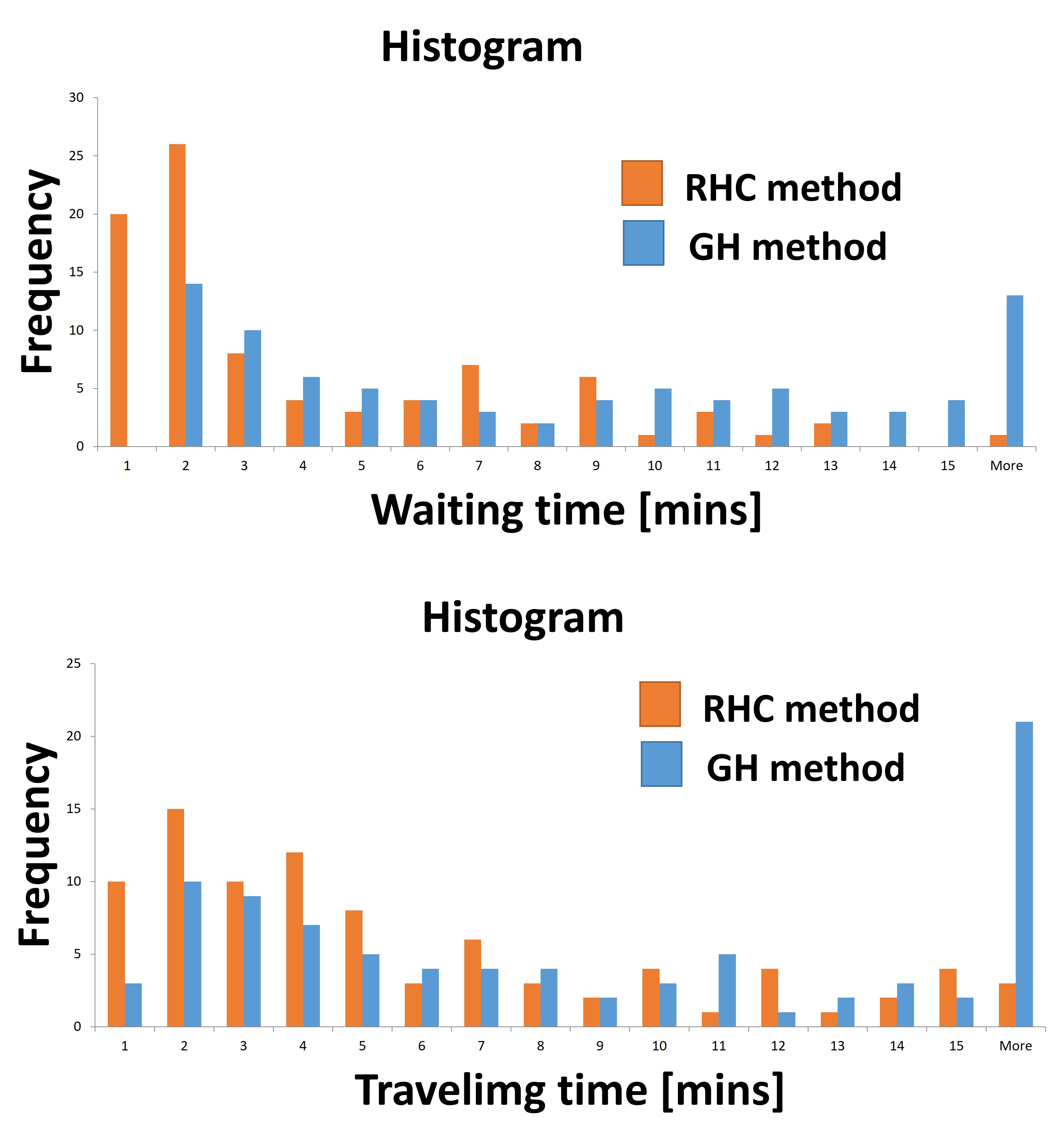
Figure 7: Comparison of waiting and traveling time histograms under RHC and GH for the Ann Arbor RSS ($\omega=0.5$).

TABLE I: Average waiting and traveling times under RHC for different weights $\omega$ in the Ann Arbor RSS

$[\omega,1-\omega]$	Waiting Time [mins]	Traveling Time [mins]	Vehicle Occupancy
$[0.05,0.95]$	6.5	4.1	1.62
$[0.5,0.5]$	6.0	5.2	2.64
$[0.95,0.05]$	6.2	5.6	3.02

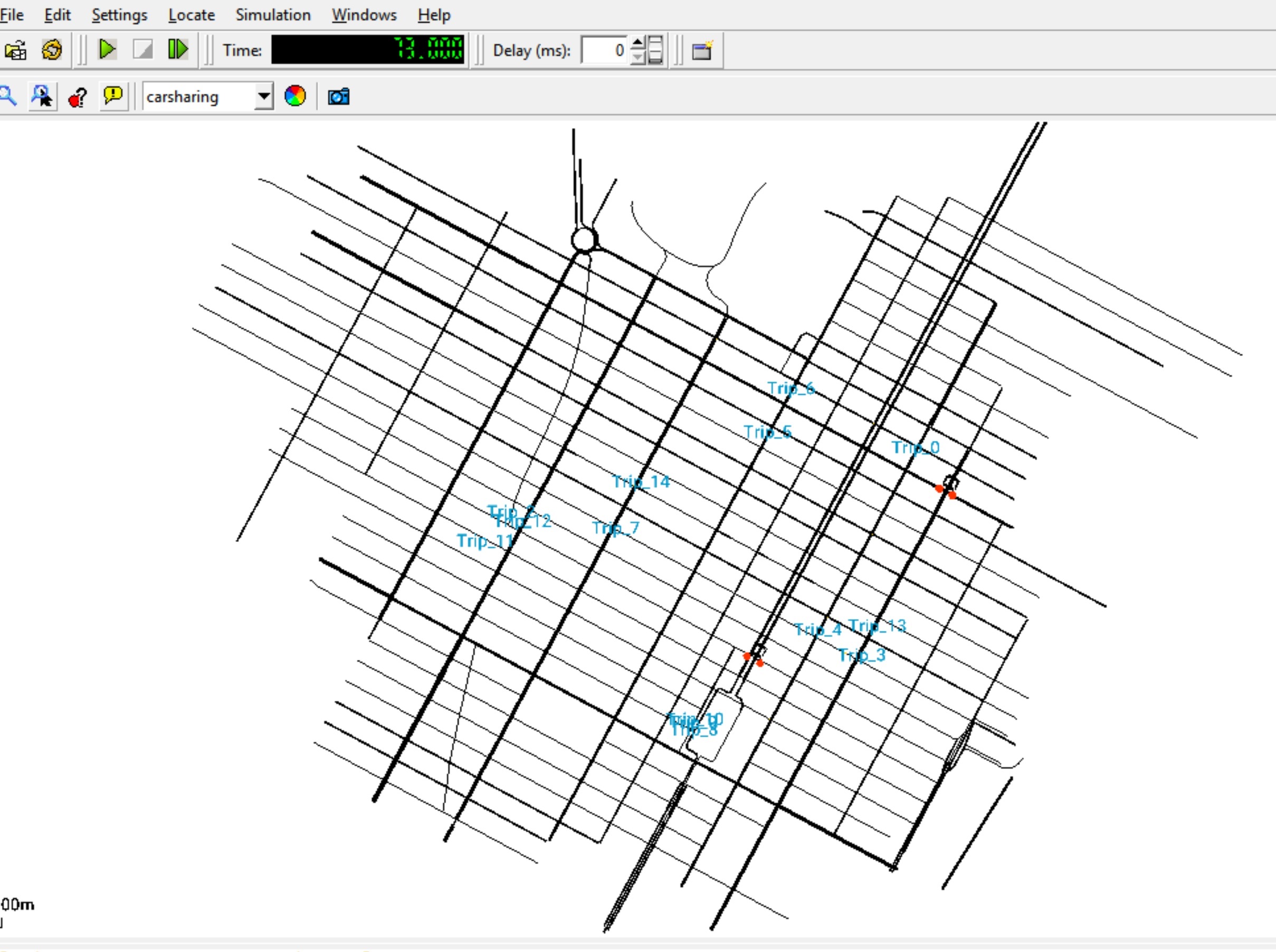
Figure 8: A RSS covering an area of $10\times 10$ blocks in New York City.

TABLE II: Average waiting and traveling time [mins] comparisons for different RSS control methods in the Ann Arbor RSS when $\omega=0.5$

Method	Waiting Time	Traveling Time	Weighted Sum in (3)
RHC	6.5	4.1	0.113
GH	9.6	9.7	0.205

TABLE III: Average waiting and traveling time [mins] comparisons for different numbers of vehicles in the Ann Arbor RSS when $\omega=0.5$ under the RHC method

Vehicle Numbers	Waiting Time	Traveling Time	Vehicle Occupancy	Weighted Sum in (3)
4	11.0	5.5	2.93	0.176
7	6.5	4.1	2.64	0.113

V-B RHC for a RSS in the New York City map

A RSS covering an area of $10\times 10$ blocks in New York City is shown in Fig.8. In this case, we generate passenger arrivals based on actual data from the NYC Taxi and Limousine Commission which provides exact timing of arrivals and the associated origins and destinations. We pre-loaded $8$ vehicles and run the simulations until $50$ passengers are served based on actual data from a weekday of January, 2016 (the approximate passenger rate is $16$ passengers/min). All other RSS settings are the same as before.

TABLE IV: Average waiting and traveling times under RHC for different weights $\omega$ in the New York City RSS with $8$ vehicles.

$[\omega,1-\omega]$	Waiting Time [mins]	Traveling Time [mins]	Vehicle Occupancy
$[0.05,0.95]$	9.1	7.8	1.96
$[0.5,0.5]$	11.9	9.0	2.59
$[0.95,0.05]$	10.3	10.2	3.06

Figure 9: Waiting and traveling time histograms under different weights $\omega$ for the New York City RSS with $8$ vehicles.

TABLE V: Average waiting and traveling time [mins] comparisons for different RSS control methods in the New York City RSS with $8$ vehicles and $\omega=0.5$.

Method	Waiting Time	Traveling Time	Weighted Sum in (3)
RHC	11.9	9.0	0.222
GH	21.5	17.0	0.410

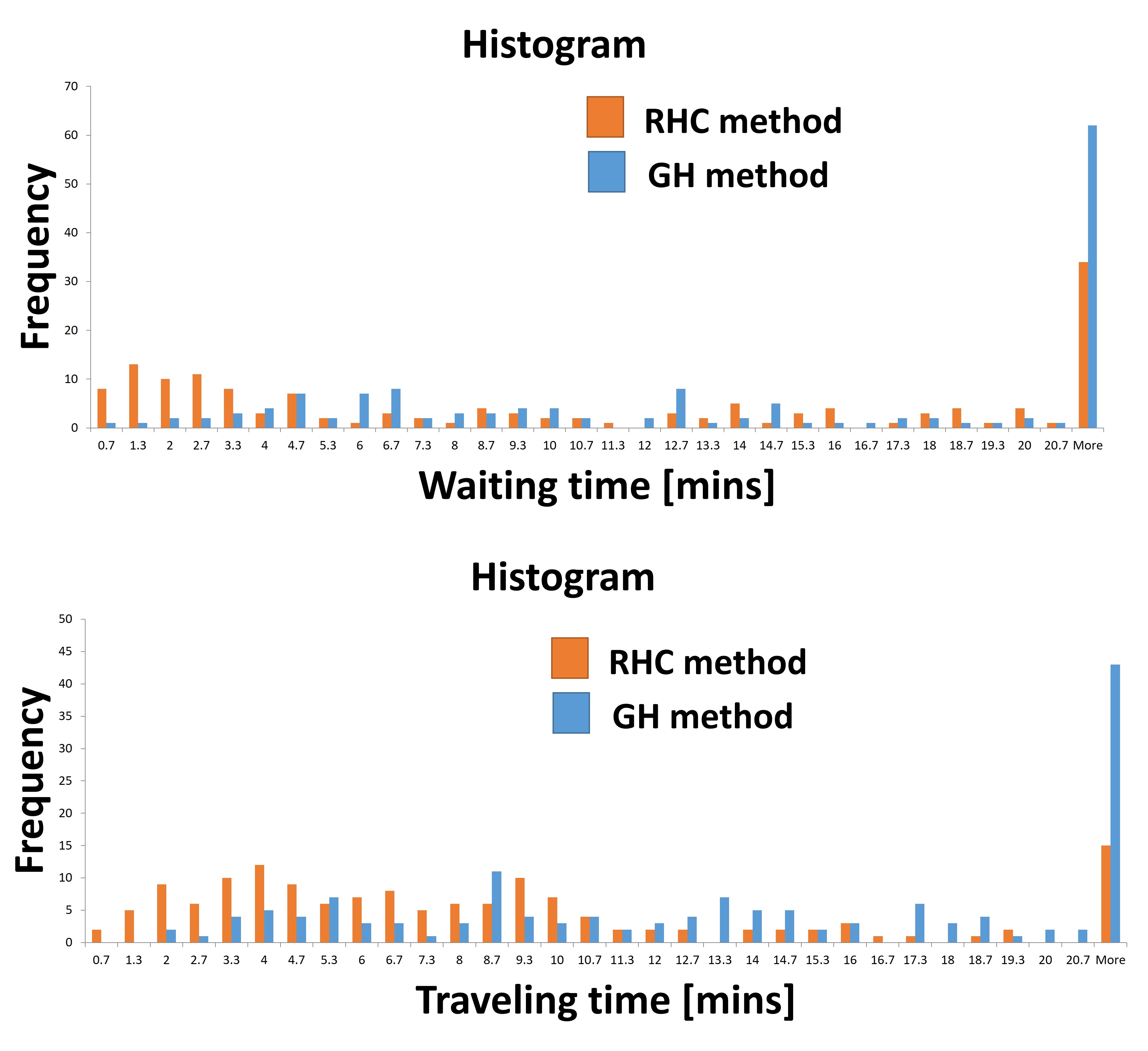
Figure 10: Comparison of waiting and traveling time histograms under RHC and GH in the New York City RSS with $8$ vehicles.

Figure 11: Waiting and traveling time histograms under different weights $\omega$ for the New York City RSS with $28$ vehicles.

TABLE VI: Average waiting and traveling times under RHC for different weights $\omega$ in the New York City RSS with $28$ vehicles.

$[\omega,1-\omega]$	Waiting time [mins]	Traveling time [mins]	Vehicle Occupancy
$[0.05,0.95]$	4.1	8.1	2.07
$[0.5,0.5]$	5.2	12.4	2.79
$[0.95,0.05]$	7.0	12.6	2.83

TABLE VII: Average waiting and traveling time [mins] comparisons under RHC and GH in the New York City RSS with $28$ vehicles and $\omega=0.5$.

Method	Waiting time	Traveling time	Weighted Sum in (3)
RHC	5.2	12.4	0.187
GH	16.1	16.6	0.348

Figure 12: Comparisons of waiting and traveling time histograms between the RHC and GH methods in the New York City RSS when the vehicle number is $28$.

In Table IV, the average waiting and traveling times under RHC are shown for different weights $\omega$ in the New York City RSS. The results are averaged over three independent simulation runs. The first column of Table IV shows different values of the weights $\omega$ as defined in (3) specifying the relative importance assigned to passenger waiting and traveling resepctively. As in the case of the Ann Arbor RSS, emphasizing waiting results in larger vehicle occupancy with longer average travel times. In Fig. 9 we provide the waiting and traveling time histograms for all cases in Table IV.

In Table V, we compare RHC with $\omega=0.5$ with the aforementioned greedy heuristic algorithm GH in terms of the average waiting and traveling times. We can see once again that the RHC algorithm achieves a substantially better performance. In Fig.10 we compare the associated waiting and traveling time histograms for RHC relative to GH.

We have also tested a relatively long RSS operation based on actual passenger data from a weekday of January 2016 which is the same as before for the shorter time intervals. We pre-loaded $28$ vehicles and run simulations until $160$ passengers are served. All other settings are the same as before.

Table VI shows the associated waiting and traveling times under different weights with similar results as before. Figure 11 shows the associated waiting and traveling time histograms for all cases in Table VI.

In Table VII, we compare RHC to the GH algorithm in terms of the average waiting and traveling times with results consistent with those of Table V.

TABLE VIII: Average waiting and traveling time [mins] comparisons for different numbers of vehicles in the New York City RSS when $\omega=0.5$ and the delivered passenger number is $160$ under the RHC method

Vehicle Numbers	Waiting Time	Traveling Time	Vehicle Occupancy	Weighted Sum in (3)
28	5.2	12.4	2.79	0.187
38	3.5	10.7	2.31	0.151

TABLE IX: Average real execution time for our RHC ALGO. when $\omega=0.5$

Vehicle Numbers	Passenger Numbers	Average Execution Time [sec]
8	50	3
28	160	17
38	160	19

Table VIII compares different vehicle numbers when the delivered passenger number is $160$ showing waiting and traveling times, vehicle occupancy and the objective in (3) whose performance is consistent with that of Table III.

Table IX shows real execution times for our RHC regarding different vehicle and passenger numbers.

TABLE X: Average waiting and traveling time [mins] comparisons under RHC and GH in the New York City RSS with $38$ vehicles and $\omega=0.5$.

Method	Waiting time	Traveling time	Weighted Sum in (3)
RHC	19.1	13.7	0.349
GH	61.4	19.0	0.855

Finally, we tested a relatively longer RSS operation with $38$ vehicles based on the same actual passenger data as before which generates $1000$ passengers over approximately $1.2$ ’real’ operation hours. Simulations will not end until $900$ passengers are delivered. In Table X, we compare RHC to the GH algorithm in terms of the average waiting and traveling times with results consistent with those of Table V.

VI Conclusions and Future Work

An event-driven RHC scheme is developed for a RSS where vehicles are shared to pick up ad drop off passengers so as to minimize a weighted sum of passenger waiting and traveling times. The RSS is modeled as a discrete event system whose event-driven nature significantly reduces the complexity of the vehicle assignment problem, thus enabling its implementation in a real-time context. Simulation results adopting actual city maps and real taxi traffic data show the effectiveness of the RHC controller in terms of real-time implementation and performance relative to known greedy heuristics. In our ongoing work, an important problem we are considering is where to optimally position idle vehicles so that they are best used upon receiving future calls. Moreover, depending on real execution times of our RHC algorithm (see Table IX), we will use this information as a rational measure for decomposing a map into regions such that within each region the RHC vehicle assignment response times remain manageable.

References

- [1] D. Schrank, T. Lomax, and B. E. TTI’s, “Urban mobility report. texas transportation institute, the texas a and m university system, 2007,” 2011.
- [2] N. Agatz, A. Erera, M. Savelsbergh, and X. Wang, “Optimization for dynamic ride-sharing: A review,” European Journal of Operational Research, vol. 223, no. 2, pp. 295–303, 2012.
- [3] X. Chen, F. Miao, G. J. Pappas, and V. Preciado, “Hierarchical data-driven vehicle dispatch and ride-sharing,” in Decision and Control (CDC), 2017 IEEE 56th Annual Conference on. IEEE, 2017, pp. 4458–4463.
- [4] N. A. Agatz, A. L. Erera, M. W. Savelsbergh, and X. Wang, “Dynamic ride-sharing: A simulation study in metro atlanta,” Transportation Research Part B: Methodological, vol. 45, no. 9, pp. 1450–1464, 2011.
- [5] P. Santi, G. Resta, M. Szell, S. Sobolevsky, S. H. Strogatz, and C. Ratti, “Quantifying the benefits of vehicle pooling with shareability networks,” Proceedings of the National Academy of Sciences, vol. 111, no. 37, pp. 13 290–13 294, 2014.
- [6] G. Berbeglia, J.-F. Cordeau, and G. Laporte, “Dynamic pickup and delivery problems,” European journal of operational research, vol. 202, no. 1, pp. 8–15, 2010.
- [7] J. Alonso-Mora, S. Samaranayake, A. Wallar, E. Frazzoli, and D. Rus, “On-demand high-capacity ride-sharing via dynamic trip-vehicle assignment,” Proceedings of the National Academy of Sciences, vol. 114, no. 3, pp. 462–467, 2017.
- [8] G. C. Calafiore, C. Novara, F. Portigliotti, and A. Rizzo, “A flow optimization approach for the rebalancing of mobility on demand systems,” in Decision and Control (CDC), 2017 IEEE 56th Annual Conference on. IEEE, 2017, pp. 5684–5689.
- [9] M. Tsao, R. Iglesias, and M. Pavone, “Stochastic model predictive control for autonomous mobility on demand,” arXiv preprint arXiv:1804.11074, 2018.
- [10] M. Salazar, F. Rossi, M. Schiffer, C. H. Onder, and M. Pavone, “On the interaction between autonomous mobility-on-demand and public transportation systems,” arXiv preprint arXiv:1804.11278, 2018.
- [11] D. P. Bertsekas, D. P. Bertsekas, D. P. Bertsekas, and D. P. Bertsekas, Dynamic programming and optimal control. Athena scientific Belmont, MA, 2005, vol. 1, no. 3.
- [12] E. F. Camacho and C. B. Alba, Model predictive control. Springer Science & Business Media, 2013.
- [13] W. Li and C. G. Cassandras, “A cooperative receding horizon controller for multivehicle uncertain environments,” IEEE Transactions on Automatic Control, vol. 51, no. 2, pp. 242–257, 2006.
- [14] Y. Khazaeni and C. G. Cassandras, “Event-driven cooperative receding horizon control for multi-agent systems in uncertain environments,” IEEE Transactions on Control of Network Systems, 2016.
- [15] J. S. Farris, “Estimating phylogenetic trees from distance matrices,” The American Naturalist, vol. 106, no. 951, pp. 645–668, 1972.
- [16] G. A. C. (DLR). (2017) Simulation of urban mobility. [Online]. Available: http://www.sumo.dlr.de/userdoc/Contact.html