A comprehensive spectroscopic and photometric analysis of DA and DB white dwarfs from SDSS and Gaia

Abstract

We present a detailed spectroscopic and photometric analysis of DA and DB white dwarfs drawn from the Sloan Digital Sky Survey with trigonometric parallax measurements available from the Gaia mission. The temperature and mass scales obtained from fits to $ugriz$ photometry appear reasonable for both DA and DB stars, with almost identical mean masses of $\langle M\rangle=0.617~{}M_{\odot}$ and $0.620~{}M_{\odot}$, respectively. The comparison with similar results obtained from spectroscopy reveals several problems with our model spectra for both pure hydrogen and pure helium compositions. In particular, we find that the spectroscopic temperatures of DA stars exceed the photometric values by $\sim$10% above $T_{\rm eff}\sim 14,000$ K, while for DB white dwarfs, we observe large differences between photometric and spectroscopic masses below $T_{\rm eff}\sim 16,000$ K. We attribute these discrepancies to the inaccurate treatment of Stark and van der Waals broadening in our model spectra, respectively. Despite these problems, the mean masses derived from spectroscopy — $\langle M\rangle=0.615~{}M_{\odot}$ and $0.625~{}M_{\odot}$ for the DA and DB stars, respectively — agree extremely well with those obtained from photometry. Our analysis also reveals the presence of several unresolved double degenerate binaries, including DA+DA, DB+DB, DA+DB, and even DA+DC systems. We finally take advantage of the Gaia parallaxes to test the theoretical mass-radius relation for white dwarfs. We find that 65% of the white dwarfs are consistent within the 1$\sigma$ confidence level with the predictions of the mass-radius relation, thus providing strong support to the theory of stellar degeneracy.

1 Introduction

Our understanding of white dwarf stars relies heavily on the determination of their physical parameters, such as effective temperature, surface gravity, luminosity, mass, radius, atmospheric composition, and cooling age. Several independent methods have been developed over the years to measure directly some of these parameters, while others are obtained indirectly through detailed evolutionary models.

The most widely used method, at least until now, to measure the effective temperature ($T_{\rm eff}$) and the surface gravity ($\log g$) of white dwarfs involves the comparison of the observed and model spectra, known as the spectroscopic technique. First applied to a large sample of DA stars by Bergeron et al. (1992), this technique has been used repeatedly since then in several other studies (see, e.g., Liebert et al. 2005, Koester et al. 2009a, Koester et al. 2009b, Tremblay et al. 2011, Gianninas et al. 2011, Genest-Beaulieu & Bergeron 2014). A similar approach has also been applied in the context of DB white dwarfs (Eisenstein et al. 2006, Voss et al. 2007, Bergeron et al. 2011, Koester & Kepler 2015, Rolland et al. 2018); in this case, the hydrogen abundance is also being measured spectroscopically.

Another method that can be applied to large ensembles of white dwarfs is the photometric technique, where the observed energy distribution, built from magnitudes in various bandpasses, is compared to the predictions from model atmospheres (see, e.g., Bergeron et al., 1997). This method yields the effective temperature and the solid angle $\pi(R/D)^{2}$ of the star; if the trigonometric parallax (or distance) is known, the radius can be obtained directly. Until recently, trigonometric parallaxes were available for only a few hundreds, mostly cool white dwarfs (Bergeron et al. 2001, Holberg et al. 2012, Tremblay et al. 2017, Bédard et al. 2017). In the absence of trigonometric parallax measurements, one usually assumes a value of $\log g=8$, in which case the photometric method can be applied to large white dwarf samples, such as those identified in the Sloan Digital Sky Survey (SDSS, Genest-Beaulieu & Bergeron 2014). In some situations, the photometric technique is the only method applicable, for example for cool white dwarfs, which present no absorption features.

With either the spectroscopic or photometric techniques, the mass of the white dwarf can only be obtained from detailed evolutionary models, which provide the required temperature-dependent relation between the mass and the radius, as well as cooling ages. This theoretical mass-radius relation for white dwarfs has recently been tested, but only for relatively small samples (Tremblay et al. 2017, Parsons et al. 2017, Bédard et al. 2017), a situation that is about to change by taking advantage of the recently measured trigonometric parallaxes from Gaia (Gaia Collaboration et al., 2018).

One of the most important issue regarding both the spectroscopic and photometric techniques is the precision and accuracy of each method. Statistically speaking, the precision of the method describes random errors, a measure of statistical variability, repeatability, or reproducibility of the measurement, while the accuracy represents the proximity of the measurements to the true value being measured, in our case, the true $T_{\rm eff}$ and $\log g$ (or mass) values. It has been argued repeatedly in the literature that the spectroscopic technique yields more precise atmospheric parameters than the photometric technique, in general because of the moderate quality of photometric and parallax measurements. However, the exquisite parallax data from Gaia and photometric data from SDSS or Pan-STARRS may change this picture drastically in favor of the photometric approach.

Another advantage of the photometric technique is that the synthetic photometry is less sensitive to the input physics included in the model atmospheres. Indeed, the shape and strength of the spectral lines are affected by a number of factors (line broadening, convective energy transport, etc.), which in turn affect the atmospheric parameters measured spectroscopically. One well-known example is the so-called high-$\log g$ problem in cool DA white dwarfs, which was explained by an inadequate treatment of convection in standard 1D model atmospheres (Tremblay et al., 2013).

The question of the precision and accuracy of the spectroscopic and photometric methods using various white dwarf samples and photometric data sets has been discussed at length by Tremblay et al. (2019, see also ). Because of the utmost importance of this issue for the white dwarf field, and also because of our different approach to the problem, we present in this paper our own independent assessment of the internal consistency between both fitting techniques by comparing the atmospheric and physical parameters of DA and DB white dwarfs obtained from spectroscopy with those derived from the photometric technique. The white dwarf samples used in this study are presented in Section 2, followed by a brief description of our models in Section 3. Our photometric and spectroscopic analyses are presented in Sections 4 and 5, respectively. Section 6 is dedicated to the comparison of the atmospheric parameters obtained from photometry and spectroscopy. Using these results, the theoretical mass-radius relation is then put to the test in Section 7. We conclude in Section 8.

2 Sample

The primary goal of this study is to compare the atmospheric parameters of DA and DB white dwarfs obtained from different techniques and data types. Given that the Sloan Digital Sky Survey (SDSS) provides photometry and spectroscopy for over 30,000 white dwarfs, we base our analysis on this particular data set. We started by retrieving all spectroscopic and photometric data for all DA and DB white dwarfs — including all subtypes (DAH, DB:, DBZ, etc.) — spectroscopically identified in the SDSS, up to the Data Release 12 (Kleinman et al., 2013; Kepler et al., 2015a, b). This represents a total of 27,217 DA and 2227 DB spectra, with corresponding $ugriz$ photometric data sets. We also want to take advantage of the Gaia DR2 catalog (Gaia Collaboration et al., 2018), which contains precise trigonometric parallax measurements for a large number of SDSS objects. In order to ensure that the atmospheric parameters we derive are reliable, we need to apply a few criteria to keep only the best SDSS and Gaia data sets.

We first removed every object with a spectral type indicating a magnetic object (H), a known companion (+ and/or M), emission lines (E), or an uncertain spectral type (:). For the DA sample, we also removed any spectral type indicating the presence of helium (B or O) or metals (Z). Therefore, our sample contains only the spectral types DA, DB, DBA(Z), and DBZ(A). We then applied a lower limit on the signal-to-noise ratio (S/N) of the SDSS optical spectra. Given the very large number of DA white dwarfs, we chose to keep only those with ${\rm S/N}\geq 25$. For the DB white dwarfs, which are not as common as DA stars, we chose to set the limit at a lower value of ${\rm S/N}\geq 10$. The S/N distribution of spectra in our sample is displayed in Figure 1. Finally, we kept only the objects with Gaia parallax measurements more precise than 10% ($\sigma_{\pi}/\pi\leq 0.1$).

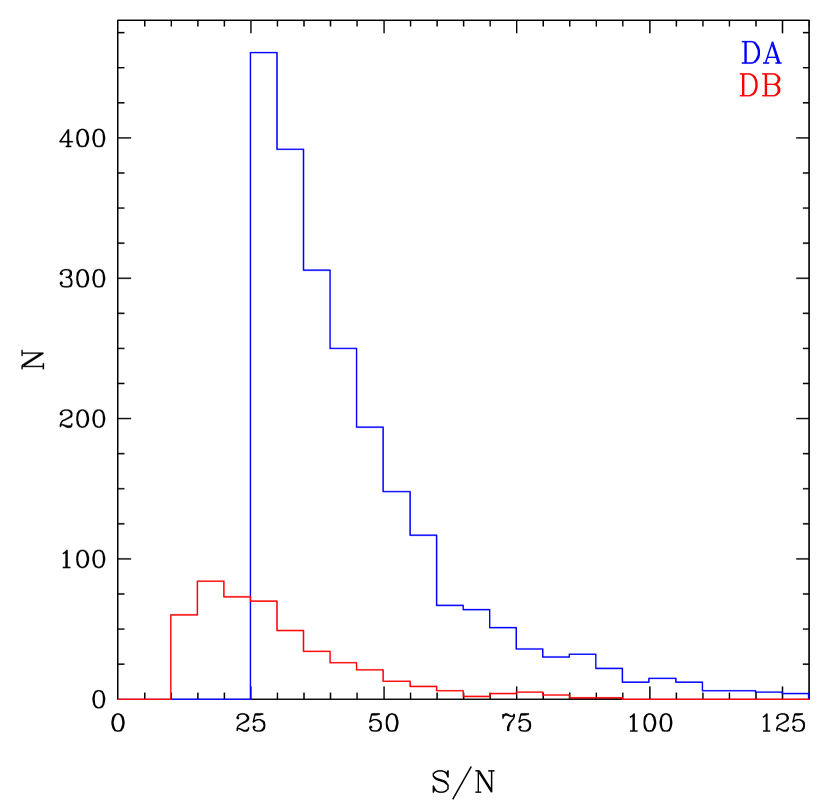
Figure 1: Distribution of signal-to-noise ratios of the DA (blue) and DB (red) white dwarfs in our sample.

After applying all these criteria, we are left with 2236 and 461 individual spectra and corresponding $ugriz$ data sets for DA and DB white dwarfs, respectively. Since the calibration algorithm has changed between DR7 and DR8, and that the $ugriz$ zeropoints have been recalibrated in DR13, we use the $ugriz$ magnitudes from the SDSS DR14 instead of the values given in the aforementioned catalogs.

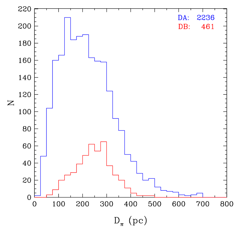
Figure 2: Distribution of parallactic distances for the DA (blue) and DB (red) white dwarfs in our sample.

Figure 2 presents the distribution of the white dwarfs in our sample as a function of distance and spectral type. We note that most of the objects in our sample are located at large distances where interstellar reddening becomes important ($D\gtrsim 100$ pc). This will be discussed in section 4.1.

3 Theoretical Framework

Since our sample contains both DA and DB white dwarfs, we require two different grids of model atmospheres and synthetic spectra.

3.1 DA Model Atmospheres

Our pure hydrogen grid for the DA stars is calculated with two different codes. For $T_{\rm eff}<30,000~{}{\rm K}$, we use the LTE version described at length in Tremblay & Bergeron (2009). Convective energy transport, which becomes important below $T_{\rm eff}\sim 15,000~{}{\rm K}$, is treated with the ML2/$\alpha=0.7$ version of the mixing-length theory (MLT). The adopted parameterization of the MLT is important, particularly for cool DA white dwarfs, and it affects mostly the atmospheric parameters determined from spectroscopic data (see section 5.3). Above 30,000 K, NLTE effects are taken into account using TLUSTY (Hubeny & Lanz, 1995). Combining both grids, we obtain model spectra ranging from $T_{\rm eff}=1500~{}{\rm K}$ up to $120,000~{}{\rm K}$, with surface gravities between $\log g=6.5$ and $9.0$. Note that both model grids rely on the improved Stark profiles of Tremblay & Bergeron (2009).

3.2 DB/DBA Model Atmospheres

Our DB/DBA model grid is similar to that described in Bergeron et al. (2011) (but see section 5.2). These models are in LTE and calculated using the ML2/$\alpha=1.25$ parameterization of the MLT. Our grid covers effective temperatures between 11,000 K and 50,000 K, surface gravities ranging from $\log g=7.0$ to $9.0$, and hydrogen abundances from $\log N({\rm H})/N({\rm He})=-6.5$ to $-2.0$, and an additional pure helium grid.

Below $T_{\rm eff}\sim 16,000$ K, He i line broadening by neutral particles becomes important. We can divide this into two parts: van der Waals and resonance broadening. In our models, these two broadening mechanisms are combined following the procedure described in detail by Beauchamp (1995), which we summarize here. Resonance broadening is treated according to the theory of Ali & Griem (1965), while van der Waals broadening requires a more elaborate approach. The width of the Lorentzian profile ($\omega_{\rm vdW}$) is calculated twice, once with the theory described in Unsold (1955), and the second time by following the approach discussed in Deridder & van Rensbergen (1976). The Deridder & van Rensbergen theory systematically predicts a larger profile if the initial and final effective quantum numbers of the transition are higher than 2 or 3. Since they used the Smirnov potential, which becomes invalid below these numbers, we keep the following conservative value for the width of the Lorentzian profile:

$$\omega_{\rm vdW}={\rm max}(\omega_{\rm Unsold},\omega_{\rm Deridder})\ .$$ (1)

It was also found empirically by Beauchamp (1995) that the neutral helium lines of cool DB stars at $\lambda=4121$ Å and 4713 Å could be better reproduced it they were strictly treated within the Unsold (1955) theory, which is the procedure we adopt here as well.

Finally, Lewis (1967) found that the combination of the resonance and van der Waals broadening led to a profile with $\omega_{\rm neutral}\sim 0.6-0.8\,(\omega_{\rm resonance}+\omega_{\rm vdW})$. However, that study was only valid for temperatures around 100 K, hardly applicable to our DB models. Therefore, the conservative value of

$$\omega_{\rm neutral}={\rm max}(\omega_{\rm resonance},\omega_{\rm vdW})$$ (2)

is adopted instead. For simplicity, we will refer to the above procedure as the Deridder & van Rensbergen theory.

Note that more recent self-broadening calculations of helium lines have been performed by Leo et al. (1995), but their results are only available at temperatures of $T=80~{}{\rm K}$ and $300~{}{\rm K}$, hardly applicable in the context of our DB models, as before.

4 Photometric Analysis

The first step in our analysis is to measure the atmospheric and physical parameters derived from photometry. Before presenting the results, we first describe the technique used to determine these parameters, and we also explore the effects of the presence of atmospheric hydrogen on the photometric solutions of DB white dwarfs.

4.1 Photometric Technique

The photometric technique relies on the energy distribution to measure the effective temperature and stellar radius. We use here the method described at length in Bergeron et al. (1997), which is the same for both DA and DB stars. Since we are using the SDSS $ugriz$ photometry, we first need to apply the corrections to the $u$, $i$, and $z$ bands to account for the transformation from the SDSS to the AB magnitude system. These corrections, given in Eisenstein et al. (2006), are

$$\begin{split}u&=u_{\rm SDSS}-0.040\\ i&=i_{\rm SDSS}+0.015\\ z&=z_{\rm SDSS}+0.030\end{split}$$ (3)

For completeness, we repeated the experiment displayed in Figure 8 of Genest-Beaulieu & Bergeron (2014) where observed magnitudes are compared with those predicted by the photometric technique, and we found that the above constants are still appropriate, and lead to a better agreement between bots sets of magnitudes.

One important aspect to consider while dealing with photometric observations is interstellar reddening, which becomes important for $D\gtrsim 100$ pc. As can be seen from Figure 2, the majority of our objects are located beyond 100 pc, implying that interstellar extinction cannot be neglected in our analysis. The procedure used here is based on the approach described by Harris et al. (2006), where the extinction is assumed to be negligible for stars with distances less than 100 pc, to be maximum for those located at $|z|>250$ pc from the galactic plane, and to vary linearly along the line of sight between these two regimes. We also explore in Section 6.1 an alternative procedure proposed by Gentile Fusillo et al. (2019). Since the trigonometric parallax is known for every object in our sample, magnitudes can be dereddened directly. This procedure is accomplished using the $E(B-V)$ values from Schlafly & Finkbeiner (2011).

Every dereddened magnitude $m_{\nu}$ is then converted into an average flux $f^{m}_{\nu}$ using the relation

$$m_{\nu}=-2.5\log f^{m}_{\nu}-48.60$$ (4)

where

$$f^{m}_{\nu}=\frac{\int f_{\nu}S_{m}(\nu)\,d\log\nu}{\int S_{m}(\nu)\,d\log\nu}\ ,$$ (5)

and where $f_{\nu}$ is the monochromatic flux from the star received at Earth, and $S_{m}(\nu)$ is the total system response, including atmospheric transmission and mirror reflectance.

The same conversion is performed using our synthetic spectra. We obtain the average synthetic fluxes, $H_{\nu}^{m}$, by substituting $f_{\nu}$ in equation 5 with the monochromatic Eddington flux $H_{\nu}$. The average observed and model fluxes are related through the equation

$$f^{m}_{\nu}=4\pi\left(R/D\right)^{2}H_{\nu}^{m}$$ (6)

where $R$ is the radius of the white dwarf, and $D$ its distance from Earth. We then proceed to minimize the $\chi^{2}$ value, which is defined in terms of the difference between observed and model fluxes over all bandpasses, properly weighted by the photometric uncertainties. Our minimization procedure relies on the non-linear least-squares method of Levenberg-Marquardt, described in Press et al. (1986), which is based on a steepest descent method. This first step is done by assuming a surface gravity of $\log g=8.0$. This yields an estimate of the effective temperature, $T_{\rm eff}$, and the solid angle, $\pi\left(R/D\right)^{2}$ — or the radius $R$ of the star since $D$ is known from the trigonometric parallax. Evolutionary models are then used to obtain the stellar mass $M$, and a new estimate of the surface gravity, which will be different from our initial assumption of $\log g=8.0$. The entire fitting procedure is then repeated until all parameters are consistent. The uncertainties associated with the fitted parameters are obtained directly from the covariance matrix of the Levenberg-Marquardt minimization procedure (see Press et al. 1986). Here we rely on C/O-core envelope models similar to those described in Fontaine et al. (2001) with thick hydrogen layers of $q({\rm H})\equiv M_{\rm H}/M_{\star}=10^{-4}$ for DA stars, and much thinner hydrogen layers of only $q({\rm H})=10^{-10}$ for DB stars, given that such thin layers are representative of helium-atmosphere white dwarfs. Finally, depending on the spectral type, we use either pure hydrogen, pure helium, or mixed H/He model atmospheres (see section 4.2). Examples of the photometric technique for both a DA and a DBA white dwarf are illustrated in Figure 3.

Figure 3: Examples of the photometric technique for the DA white dwarf SDSS J110515.32+001626.10 (top) and the DBA SDSS J083542.23+040817.50 (bottom). The error bars represent the observed data, while the best-fit model is shown by the filled circles. The resulting atmospheric parameters are given in each panel.

The precision of the photometric technique is limited by the sensitivity of the photometric measurements (here SDSS $ugriz$) to variations in effective temperature. At high $T_{\rm eff}$ values, the energy distribution sampled by the $ugriz$ photometry is in the Rayleigh-Jeans regime. This is illustrated in Figure 4 where we show magnitude differences (i.e., color indices) with respect to the $g$ magnitude for all SDSS bandpasses, as a function of effective temperature and atmospheric composition. In the case of pure hydrogen atmospheres, the energy distribution varies considerably up to $T_{\rm eff}\sim 35,000~{}{\rm K}$, and very little above this temperature. This means that the photometric technique becomes less reliable above 35,000 K for DA white dwarfs. The situation is similar in the case of DB stars. For DA stars, the Balmer jump affects the $u-g$ color index significantly, which can be observed here as the flat plateau between $\sim$8000 K and 15,000 K. Also of interest is the behavior below $\sim$5000 K where collision-induced absorption by molecular hydrogen becomes important. These two features are of course not observed in pure helium atmospheres.

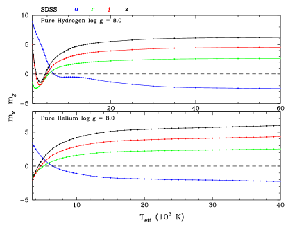
Figure 4: Magnitude differences between the SDSS $u$ (blue), $r$ (green), $i$ (red), and $z$ (black) bands and the SDSS $g$ band, as a function of effective temperature, for pure hydrogen (top) and pure helium (bottom) models at $\log g=8.0$ (note the difference in temperature scales). The dots correspond to individual model values.

4.2 Effect of the Presence of Hydrogen on the Photometric Solutions

When using the photometric technique, one usually assumes either pure hydrogen or pure helium atmospheres to determine the stellar parameters. However, most DB stars contain a certain amount of hydrogen (Koester & Kepler, 2015; Rolland et al., 2018). We show in Figure 5 the hydrogen abundance (or upper limits) as a function of effective temperature for all the DB and DBA stars in our sample. In some cases the hydrogen abundance can be as large as $\log N(\rm{H})/N(\rm{He})\sim-3$. Since the presence of additional free electrons in helium-rich atmospheres may affect significantly the photometric solutions — see, e.g., Figure 8 of Dufour et al. (2005) in the context of DQ white dwarfs —, we explore here the effect of the hydrogen abundance on the atmospheric parameters obtained for DBA stars using the photometric technique.

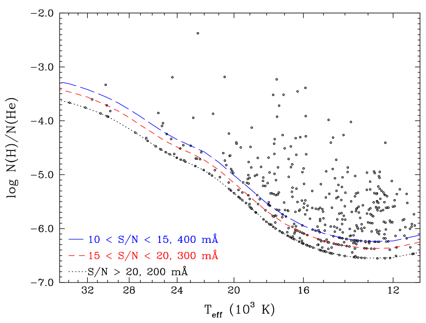
Figure 5: Spectroscopic hydrogen abundance as a function of effective temperature for the DB and DBA stars in our sample. Also shown are the H$\alpha$ detection limits for ${\rm S/N}>20$, $15<{\rm S/N}<20$, and $10<{\rm S/N}<15$, corresponding to equivalent widths (FWHM) of 200 mÅ (black, dotted line), 300 mÅ (red, short-dashed line), and 400 mÅ (blue, long-dashed line), respectively.

To do so, we use the same procedure as before, but instead of using pure helium models, we force the hydrogen abundance to the spectroscopic value. The effects on the effective temperature and stellar mass are displayed in Figure 6. The top panel shows that by using pure helium models, we tend to overestimate the effective temperature, but not significantly. For most objects, the difference in temperature is less than 1% to 2%, which is smaller than the uncertainty associated with the photometric technique. The objects for which the difference in temperature is the largest, between $\sim$2.5 and 5%, are all found below $T_{\rm eff}\sim 14,000~{}{\rm K}$, and these correspond to the few DBA stars in this temperature range with the largest hydrogen abundances around $\log N({\rm H})/N({\rm He})\sim-4.0$.

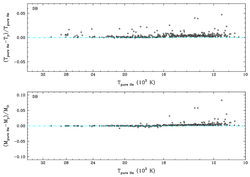
Figure 6: Top panel: Effect of the hydrogen abundance on the effective temperature determined photometrically, as a function of $T_{\rm eff}$. $T_{\rm pure~{}He}$ is the effective temperature obtained from pure helium models, while $T_{y}$ is that obtained by forcing the hydrogen abundance to the spectroscopic value. The dashed line corresponds to $T_{\rm pure~{}He}=T_{y}$. Bottom panel: Same as top panel, but for stellar masses. The cyan dashed line corresponds to $M_{\rm pure~{}He}=M_{y}$.

The bottom panel of Figure 6 shows the effect on the mass determinations. Above $T_{\rm eff}\sim 16,000~{}{\rm K}$, the effect is completely negligible. Below this temperature, the masses obtained under the assumption of a pure helium atmosphere are slightly overestimated, by about 0.01 $M_{\odot}$ for the bulk of our sample, but these differences can be as large as 0.05 to 0.1 $M_{\odot}$ in some cases. These correspond also to the objects that show the largest temperature differences in the upper panel. Since the luminosity $L\propto R^{2}T_{\rm eff}^{4}$, a lower temperature implies a larger radius, or a smaller mass (see also Figure 8 of Dufour et al., 2005).

Overall, we conclude that the use of mixed composition atmospheres for measuring the photometric mass and effective temperature of DBA white dwarfs yields values very similar to those obtained under the assumption of pure helium compositions. Nevertheless, to be fully consistent, we adopt in what follows the spectroscopic hydrogen abundance to measure the stellar parameters using the photometric technique.

4.3 Photometric Results

Using the photometric technique described in Section 4.1, we determined the effective temperature and stellar mass of every object in our sample. As mentioned in the previous section, for the DB/DBA stars, the hydrogen abundance (or limit) was forced to its spectroscopic value. The resulting mass distributions for the DA and DB stars in our sample are displayed as a function of effective temperature in the top panels of Figures 7 and 8, respectively.

Below $T_{\rm eff}\sim 45,000$ K, the mass distribution for the DA white dwarfs appears well-centered around 0.6 $M_{\odot}$, regardless of the effective temperature. This is expected since it is believed that white dwarfs cool with a constant mass. Above this temperature, however, the DA stars in our sample appear to have larger than average masses, around $\sim 0.7~{}M_{\odot}$. This is probably due to the limitations of the photometric technique using $ugriz$ data in this temperature range (see Figure 4). The distribution of objects in the upper panel of Figure 7 also appears uniform as a function of $T_{\rm eff}$, i.e., there are no gaps in the temperature distribution, except perhaps around 12,000 K where there seems to be a slight depletion of objects. This might be caused by selection effects in the SDSS, or it could also be due to spectral evolution mechanisms, such as the transformation of DA into non-DA white dwarfs resulting from convective mixing in this temperature range. But such considerations are outside the scope of this paper.

We can also identify a significant number of DA stars with very low photometric masses ($M\lesssim 0.45\ M_{\odot}$). These objects are most likely unresolved double degenerate binaries. In these cases, the object appears overluminous because of the presence of two stars in the system, and the radius determined photometrically is thus overestimated. Because of the mass-radius relation, the stellar mass inferred from this radius is underestimated. These objects will be discussed further in Sections 6.2 and 7. Finally, the mass distribution also reveals the existence of high-mass white dwarfs ($M\gtrsim 0.8M_{\odot}$). These high-mass DA stars are usually thought to be the end result of stellar mergers (Iben, 1990; Kilic et al., 2018), or alternatively, they can also be explained as a result of the initial-to-final mass relation (El-Badry et al., 2018).

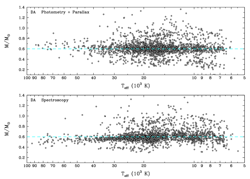
Figure 7: Stellar mass as a function of effective temperature obtained from photometry (top) and spectroscopy (bottom), for the DA white dwarfs in our sample. The dashed cyan line represents a constant mass of 0.6 $M_{\odot}$.

As for the DA white dwarfs, the mass distribution for the DB stars (top panel of Figure 8) shows a rather uniform distribution as a function of $T_{\rm eff}$, with no obvious gaps. Unlike for the DA mass distribution, however, which was centered around $\sim$0.6 $M_{\odot}$ regardless of $T_{\rm eff}$, the mean mass for DB stars appears well-centered around 0.6 $M_{\odot}$ for $T_{\rm eff}\lesssim 16,000~{}{\rm K}$, but systematically above this value at higher temperatures. Also, the most striking feature in the photometric mass distribution is that there is no significant increase in mass below $T_{\rm eff}\sim 16,000~{}{\rm K}$, in sharp contrast with the spectroscopic mass distributions reported for instance by Bergeron et al. (2011) and Koester & Kepler (2015). We come back to these points further in Sections 5.2 and 6.2.

We also note the presence of a few low-mass DB white dwarfs ($M\lesssim 0.45~{}M_{\odot}$). Again, these are most likely unresolved double degenerate candidates, which will be discussed in more detail in Sections 6.2 and 7.

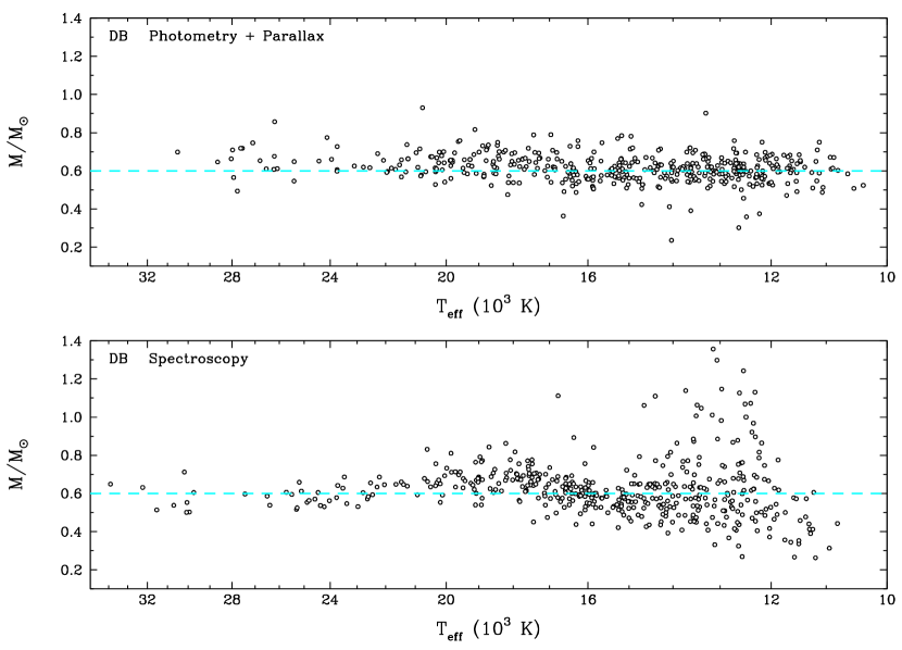
Figure 8: Same as Figure 7, but for the DB white dwarfs in our sample.

5 Spectroscopic Analysis

5.1 Spectroscopic Technique

The most widely used technique to measure the atmospheric parameters — $T_{\rm eff}$, $\log g$, and atmospheric composition — of white dwarf stars is the so-called spectroscopic technique, which relies on normalized spectral line profiles. Unlike the photometric technique, which is the same regardless of the atmospheric composition, the spectroscopic technique differs slightly depending on the spectral type of the object. We describe in turn the fitting procedures used for both DA and DB stars in our SDSS sample.

5.1.1 DA White Dwarfs

For DA white dwarfs, we use a technique similar to that described in Bergeron et al. (1992), Bergeron et al. (1995), and Liebert et al. (2005). The first step is to normalize the hydrogen lines, from H$\beta$ to H8, for both the observed and synthetic spectra, convolved with the appropriate Gaussian instrumental profile (3 Å FHWM in the case of the SDSS spectra). The comparison is then carried out in terms of these normalized line profiles only. In order to properly define the continuum on each side of the line, we use two different procedures depending on the temperature range. For $16,000~{}{\rm K}<T_{\rm eff}<9000~{}{\rm K}$, we fit the entire spectrum using a sum of pseudo-Gaussian profiles, as they reproduce quite well the spectral line profiles in this temperature range, an example of which is shown in the top right panel of Figure 9. Outside of this temperature range, we rely on our synthetic spectra to reproduce the observed spectrum, including a wavelength shift, as well as several order terms in $\lambda$ (up to $\lambda^{6}$), to obtain a smooth fitting function. This is achieved using the Levenberg-Marquardt method described above. Since the hydrogen lines reach their maximum strength around $T_{\rm eff}=14,000~{}{\rm K}$, both the cool and hot solutions are tested and the one with the lowest $\chi^{2}$ is kept. The resulting best fit is then used to normalize the line profiles to a continuum set to unity, although the atmospheric parameters obtained at this point are meaningless because of the high number of fitting parameters used in the normalization procedure. However, these $T_{\rm eff}$ and $\log g$ estimates can be used as a starting point for the full $\chi^{2}$ minimization procedure since they are usually quite close to the physical solution. This also helps us to determine on which side of the maximum line strength our object is located. In principle, the photometric temperature could also be used to distinguish between the cool and hot solutions, but we want our spectroscopic fitting procedure to be as independent as possible from the photometric approach.

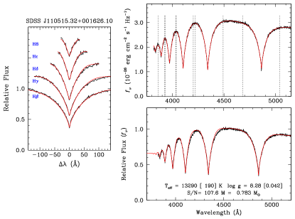
Figure 9: Example of the spectroscopic technique for the DA white dwarf SDSS J110515.32+001626.10. Top right panel: The smooth fitting function (red) used to define the continuum is plotted over the observed spectrum (black). Left panel: Best model fit (red) to the observed (normalized) hydrogen line profiles (black). Bottom right panel: Final solution (red) superposed on the observed spectrum (black), both normalized at 4600 Å. The derived stellar parameters are also given in the figure.

Once the lines are properly normalized, the effective temperature and surface gravity are determined using the Levenberg-Marquardt procedure. Finally, the 3D corrections from Tremblay et al. (2013) are applied to both $T_{\rm eff}$ and $\log g$. A full example of the fitting procedure for DA white dwarfs is presented in Figure 9.

The uncertainties associated with spectroscopic $T_{\rm eff}$ and $\log g$ values were estimated by Liebert et al. (2005) for the DA stars in the Palomar-Green survey. Multiple measurements of the same stars were used to determine that the overall errors are 1.4% in $T_{\rm eff}$ and 0.042 dex in $\log g$. Note that these values were obtained using a spectroscopic sample with ${\rm S/N}>50$. In our SDSS sample, however, most of our DA spectra have ${\rm S/N}\lesssim 50$ (see Figure 1), with very few objects at higher values. Nevertheless, we will assume here the same uncertainties as those of Liebert et al., but we keep in mind that these are most likely underestimated.

5.1.2 DB/DBA White Dwarfs

The spectroscopic technique used for the DB/DBA white dwarfs differs slightly from that used for DA stars since there is a third parameter to measure: the hydrogen abundance. We use a technique similar to that described in Bergeron et al. (2011). The normalization procedure for the DB spectra relies on our synthetic spectra to obtain a smooth fitting function used to determine the continuum, as described above for the DA stars. Again, we find a solution on each side of the maximum line strength, which occurs near 25,000 K for DB white dwarfs, and the solution with the smallest $\chi^{2}$ is used to define the continuum. As before, this normalization procedure uses too many fitting parameters for the values of $T_{\rm eff}$, $\log g$, and $\log N({\rm H})/N({\rm He})$ to be meaningful.

Once the observed spectrum is normalized, the first step is to obtain an estimate of the effective temperature and surface gravity, using the blue part of the spectrum ($\lambda=3750-5150$ Å). Keeping those parameters fixed, the hydrogen abundance is obtained by fitting the region near H$\alpha$ ($\lambda=6400-6800$ Å). For some stars, this part of the spectrum is problematic, so the hydrogen abundance is determined using H$\beta$ instead. The entire procedure is then repeated in an iterative fashion, until the value of $N({\rm H})/N({\rm He})$ has converged. In several cases, only upper limits on the hydrogen abundance could be obtained based on the absence of H$\alpha$ within the detection limit (see Figure 5). An example of the fitting procedure for a typical DBA white dwarf is shown in Figure 10.

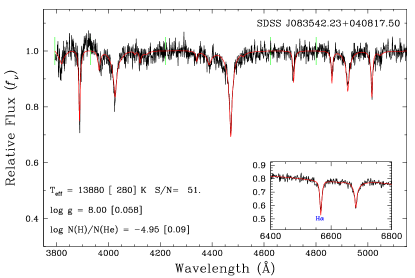
Figure 10: Example of the spectroscopic technique for the DBA white dwarf SDSS J083542.23+040817.50. The best fit (red) is plotted over the normalized observed spectrum (black). The inset shows the region near H$\alpha$ used to determine the hydrogen abundance, or upper limits. The derived atmospheric parameters are also given in the figure.

Bergeron et al. (2011) determined, in the same manner as Liebert et al. (2005), that the overall error on the effective temperature and surface gravity were 2.3% and 0.052 dex, respectively. Although we will be using those estimates, it should be noted that they determined those values with much higher signal-to-noise spectra than what is use in the present study (${\rm S/N}\gtrsim 50$ in Bergeron et al. 2011 vs ${\rm S/N}>10$ here, see Figure 1). Therefore, our uncertainties are most likely underestimated.

Cukanovaite et al. (2018) calculated a series of 3D hydrodynamical white dwarf atmosphere models with pure helium compositions, similar to those for DA stars by Tremblay et al. (2013). They also published 3D corrections to be applied to 1D spectroscopic solutions, which are found to be important in the range $T_{\rm eff}\sim 17,000~{}{\rm K}-20,000~{}{\rm K}$. However, since it is expected that the presence of hydrogen will affect these corrections, and that such calculations are currently underway, we refrain from applying any correction to our spectroscopic solutions at this stage. We will keep this in mind, however, when we compare the photometric and spectroscopic results in Section 6. Note that these more realistic 3D hydrodynamical models should not affect in any way the photometric analyses presented above for both DA and DB white dwarfs.

5.2 van der Waals Broadening in DB White Dwarfs

A well-known problem in the case of DB white dwarfs is the apparent increase in $\log g$, or mass, at low effective temperatures ($T_{\rm eff}\lesssim 15,000~{}{\rm K}$). This phenomenon has been reported repeatedly, for instance, in Beauchamp et al. (1996), Bergeron et al. (2011), and Koester & Kepler (2015). The photometric mass distribution displayed in the top panel of Figure 8 reveals that this increase in mass occurs only when the atmospheric parameters are determined using the spectroscopic technique, a conclusion also reached by Tremblay et al. (2019). A similar phenomenon was also observed in the $\log g$ distribution of cool DA stars — the so-called high-$\log g$ problem — but in this case, Tremblay et al. (2013) showed that the problem lies in the use of the mixing-length theory to treat convective energy transport, and that more realistic 3D hydrodynamical calculations could solve this high-$\log g$ problem.

The high-$\log g$ values inferred for cool DB white dwarfs most likely have a different origin, however, since in the temperature regime where the problem is observed, convection is almost completely adiabatic (Cukanovaite et al., 2018). Instead, it has been generally argued that van der Waals broadening was the source of the problem (Bergeron et al. 2011 and references therein). In their paper, Bergeron et al. (2011, see also ) erroneously mention that they used the Deridder & van Rensbergen theory to treat van der Waals broadening, as defined in Section 3.2, while they were in fact relying on the more simple theory of Unsold (1955). To clarify this situation, we fitted all the DB stars in our SDSS sample using both the Unsold and the Deridder & van Rensbergen theories, the results of which are displayed in Figure 11.

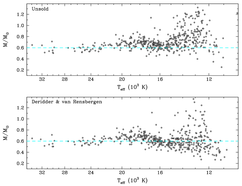
Figure 11: Spectroscopic mass distribution as a function of effective temperature for the DB white dwarfs in the SDSS sample, using the van der Waals broadening theory of Unsold (1955, top) and Deridder & van Rensbergen (bottom; as defined in Section 3.2). The dashed line in both panels corresponds to a constant mass of 0.6 $M_{\odot}$.

Our results using the Unsold theory can be compared directly with those shown, for instance, in Figure 6 of Rolland et al. (2018). Although the sample analyzed by Rolland et al. is significantly smaller than our SDSS sample, both distributions are qualitatively similar. In particular, they both show a large increase in mass below $T_{\rm eff}\sim 15,000$ K. By using instead the Deridder & van Rensbergen theory (bottom panel of Figure 11), we still find white dwarfs with large masses ($M\sim 1.2-1.3~{}M_{\odot}$) at low temperatures, but more importantly, the mass of the bulk of our sample has been reduced from a value above 0.6 $M_{\odot}$ to a value significantly below this mark. Furthermore, the mass distribution now contains several objects with low masses ($M\lesssim 0.45\ M_{\odot}$). Finally, the scatter at low temperatures remains large with both theories. Note that the stellar masses are relatively unaffected above $\sim$16,000 K, where Stark broadening dominates.

The results displayed in Figure 11 indicate that the theory of van der Waals broadening still requires significant improvement before any meaningful spectroscopic analysis of cool DB/DBA white dwarfs can be achieved. For instance, our particular choice (see Section 3.2) — based on the results of Lewis (1967) — to use $\omega_{\rm neutral}={\rm max}(\omega_{\rm resonance},\omega_{\rm vdW})$ instead of the sum of the two contributions, might not be appropriate. Mullamphy et al. (1991) indeed found that a simple sum, $\omega_{\rm neutral}=\omega_{\rm resonance}+\omega_{\rm vdW}$, provided a better agreement between theory and experiment. However, the inadequacy in the treatment of He i line broadening by neutral particles is outside the scope of this paper, and further improvements will be explored elsewhere. For the lack of a better theory for van der Waals broadening, we use in the remainder of our analysis the Deridder & van Rensbergen theory, as defined in Section 3.2.

For completeness, we show in Figure 12 the differences in effective temperature, mass, and hydrogen abundance obtained from models using the Deridder & van Rensbergen and Unsold theories, but only for the objects in our sample with $T_{\rm eff}<17,000~{}{\rm K}$. The maximum differences occur near $T_{\rm eff}\sim 13,000~{}{\rm K}$, and are of the order of 2.5% in temperature, 0.2 $M_{\odot}$ in mass, but only 0.2 dex in $\log N({\rm H})/N({\rm He})$.

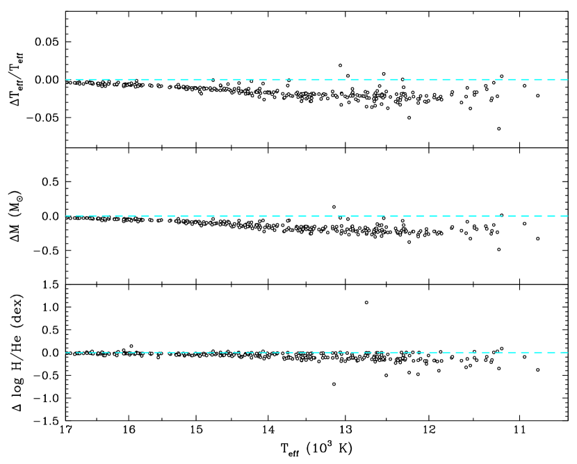
Figure 12: Differences in effective temperature, mass, and hydrogen abundances as a function of $T_{\rm eff}$ obtained between models using the van der Waals broadening theory of Deridder & van Rensbergen (as defined in Section 3.2) and the Unsold (1955) theory.

5.3 Spectroscopic Results

Using the spectroscopic techniques described in section 5.1, we measured the atmospheric parameters of all the DA and DB stars in our SDSS sample. Stellar masses were then obtained by converting the spectroscopic $\log g$ values into mass using the same evolutionary models as those described in Section 4.1. We discuss these results in turn.

The spectroscopic mass distribution for the DA white dwarfs is shown as a function of effective temperature in the bottom panel of Figure 7, which can be contrasted with the photometric distribution in the upper panel. Both distributions reveal several high-mass white dwarfs ($M\gtrsim 0.8~{}M_{\odot}$), which, as mentioned above, are believed to be the product of stellar mergers, or alternatively, the result of the initial-to-final mass relation. We also note the presence of low-mass white dwarfs ($M\lesssim 0.4~{}M_{\odot}$) in both distributions, most likely unresolved double degenerate binaries (see Section 6.2).

The spectroscopic mass distribution of DA stars shows a rather uniform distribution as a function of $T_{\rm eff}$, with the exception of an obvious gap near 14,000 K. Similar but less obvious gaps were mentioned in the photometric mass distribution as well (see Section 4.3), but these occur at different temperatures and are probably unrelated. The gap observed in the spectroscopic mass distribution of DA stars actually corresponds to the temperature where hydrogen lines reach their maximum strength. If our models predict lines that are stronger than what is actually observed, the spectroscopic technique will push the stars away from the maximum, either on the cool or hot side, to match the observed spectrum, as observed here. On the other hand, if the predicted lines are weaker than observed, stars would tend to accumulate near $T_{\rm eff}\sim 14,000~{}{\rm K}$. Both situations are illustrated in Figure 3 of Bergeron et al. (1995) where the mass distribution of bright DA stars is shown as a function of effective temperatures for different parameterizations of the MLT, which affect significantly the predicted maximum line strength. Also of importance are the adopted Stark broadening profiles used in the synthetic spectrum calculations — those of Tremblay & Bergeron (2009) in our models. The gap observed in Figure 7 suggests that Stark broadening or the treatment of convection, or even both, might need to be revisited.

There is even a third alternative explanation for the presence of this gap. Indeed, Genest-Beaulieu & Bergeron (2014) reported a similar deficit of objects near 14,000 K in the spectroscopic temperature distribution of DA stars from the SDSS (see their Section 3.4 and their Figures 14 and 15), while an accumulation of objects was observed instead when using the DA spectra from Gianninas et al. (2011). Furthermore, they also found that while the mass distribution as a function of $T_{\rm eff}$ followed a constant mean value of $\sim$0.6 $M_{\odot}$ when using the Gianninas sample, the spectroscopic masses at higher temperatures were lower than this canonical value when using SDSS spectra, as also observed here in the lower panel of Figure 7 (for $T_{\rm eff}\gtrsim 30,000~{}{\rm K}$). Based on these results, Genest-Beaulieu & Bergeron concluded that the SDSS spectra may still suffer from calibration issues.

The spectroscopic mass distribution for the DB stars, presented in the bottom panel of Figure 8, is much more complex than in the case of DA white dwarfs. The most striking detail about this distribution is the very large scatter in mass for $T_{\rm eff}\lesssim 15,000~{}{\rm K}$. This was also discussed in Section 5.2, and the most likely cause of this scatter is the improper treatment of van der Waals broadening in our model atmospheres. Also, contributing to this scatter is the lack of sensitivity of the spectroscopic technique below $T_{\rm eff}\sim 12,000~{}{\rm K}$, when the helium lines become too weak (see, e.g., Figure 3 of Rolland et al. 2018).

The spectroscopic mass distribution for DB stars also shows a significant increase in mass of $\sim$0.1 $M_{\odot}$ in the range $20,000~{}{\rm K}>T_{\rm eff}>16,000~{}{\rm K}$. As discussed above, this corresponds to the temperature range where 3D hydrodynamical effects are expected to become important in pure helium DB stars (Cukanovaite et al., 2018). Cukanovaite et al. showed that the largest differences in spectroscopic $\log g$ values inferred from both 1D and 3D models occur at $T_{\rm eff}\sim 18,000~{}{\rm K}$, and that 1D models tend to overestimate the surface gravities, and thus masses, as observed here. But as discussed above, the photometric masses also lie above 0.6 $M_{\odot}$ in the same temperature range. We come back to this point in the next section.

6 Comparison of Photometric and Spectroscopic Atmospheric Parameters

In this section we compare the effective temperatures and stellar masses obtained from the photometric and spectroscopic techniques (Sections 4 and 5) for both the DA and DB white dwarfs in our SDSS sample.

6.1 Effective Temperatures

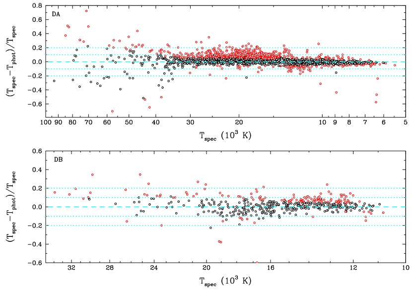
Figure 13: Differences between spectroscopic and photometric effective temperatures as a function of $T_{\rm spec}$ for the DA (top) and DB (bottom) white dwarfs in our SDSS sample. Objects with temperature differences within (outside) the 1$\sigma$ confidence level are shown in black (red). The dashed line corresponds to $T_{\rm spec}=T_{\rm phot}$, while the dotted lines show $\pm 10$% and $\pm 20$% differences in temperature.

The differences between the spectroscopic and photometric effective temperatures — $T_{\rm spec}$ and $T_{\rm phot}$ — for the DA white dwarfs in our sample are shown as a function of $T_{\rm spec}$ in the top panel of Figure 13. Here and below, we use black (red) symbols to indicate white dwarfs whose temperature estimates are within (outside) the 1$\sigma$ confidence level, where $\sigma$ is defined as the combined photometric and spectroscopic uncertainties, $\sigma^{2}\equiv\sigma^{2}_{T_{\rm phot}}+\sigma^{2}_{T_{\rm spec}}$. Using this definition, we find that 63.3% of the DA white dwarfs in our sample have temperature estimates that agree within 1$\sigma$. This is somewhat lower than expected from Gaussian statistics (68%), but as mentioned in Sections 5.1.1 and 5.1.2, we are most likely underestimating the uncertainties associated with our spectroscopic parameters, for both the DA and DB white dwarfs.

Despite this overall agreement between the photometric and spectroscopic temperatures, we can observe some obvious systematic effects in the top panel of Figure 13, which depend on the range of temperatures considered. For instance, below $T_{\rm eff}\sim 14,000$ K, as much as 76% of the objects agree within 1$\sigma$, with no obvious systematic trend. Above this temperature, however, only 58% of the sample is within 1$\sigma$, and more importantly, spectroscopic temperatures are about 5% to 10% higher than those inferred from photometry. This systematic offset also appears to be fairly constant through the entire temperature range above 14,000 K. A similar offset has been reported before by Genest-Beaulieu & Bergeron (2014, see their Figure 20 and the discussion in their Section 4) using similar SDSS photometric and spectroscopic data. The authors note that this effect is also observed (see their Figure 22) when using the DA spectra from Gianninas et al. (2011), and is thus not related to the particular use of SDSS spectra. Tremblay et al. (2019) also observed a similar systematic offset using Gaia photometry, but in their case, the offset is seen for all temperatures.

Since interstellar reddening is important for the SDSS sample, in particular for the hotter and thus intrinsically more luminous and more distant objects, we explore in Figure 14 the exact same results as in Figure 13, but this time as function of the parallactic distance $D_{\pi}$. We can see here that the systematic offset in temperature is not a function of distance, and more importantly, it is also present below 100 pc where interstellar reddening is negligible according to the dereddening procedure described in Harris et al. (2006). Gentile Fusillo et al. (2019) proposed an alternative dereddening procedure (see their Section 4) that differs slightly from that used by Harris et al., in particular for $D<100$ pc. We explore in Figure 15 the differences between these two recipes, but only for the DA stars in our sample. As can be seen, the results are virtually identical. Actually, the fraction of white dwarfs whose temperature estimates are within the 1$\sigma$ confidence level decreases from a value of 63.3% with the Harris et al. procedure, to a value of 61.2% with the Gentile Fusillo et al. approach. We thus conclude that our dereddening procedure described in Section 4.1 is probably reliable, and that it is not the source of the systematic temperature discrepancy observed in Figure 13.

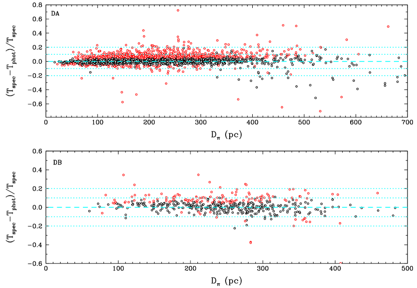
Figure 14: Same as Figure 13 but as a function of parallactic distances.

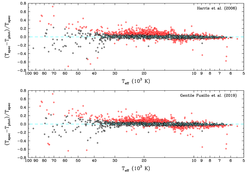
Figure 15: Same as the upper panel of Figure 13 (DA stars only), where interstellar extinction is taken into account by following the approach described by Harris et al. (2006, upper panel) and by Gentile Fusillo et al. (2019, lower panel).

One possible reason for the temperature discrepancy might be related to the physics of line broadening theory, which is likely to affect more importantly the spectroscopic parameters than those obtained from photometry, a solution also proposed by Tremblay et al. (2019). For instance, Genest-Beaulieu & Bergeron (2014) compared in their Figure 23 the photometric and spectroscopic temperatures for the DA stars in the Gianninas et al. sample, but by using model spectra calculated with the Stark profiles of Lemke (1997) — with twice the value of the critical electric microfield $\beta_{\rm crit}$ in the Hummer-Mihalas occupation probability formalism (see Bergeron et al. 1992 and references therein) — instead of those of Tremblay & Bergeron (2009) used in our analysis. They obtained a much better agreement with these older profiles above $T_{\rm eff}\sim 20,000$ K, although other systematic effects were introduced between 13,000 K and 19,000 K. Nevertheless, these results strongly suggest that Stark broadening probably needs further improvements, for instance along the lines of the promising work of Gomez et al. (2017).

The region around $T_{\rm eff}=14,000~{}{\rm K}$ in Figure 13 also appears problematic. As mentioned above, this corresponds to the temperature at which the hydrogen lines reach their maximum strength. The spectroscopic solutions in this region are particularly sensitive to the treatment of atmospheric convection, to 3D hydrodynamical effects, to the physics of Stark broadening, and even to flux calibration issues. All these effects are responsible for moving the objects around the region where the lines reach their maximum strength, and for producing the increased scatter near 14,000 K in Figure 13. It is even possible that for some objects, the spectroscopic technique did not pick the correct solution, cool or hot, in particular when both are close to the photometric temperature, in which case it is virtually impossible to discriminate between both solutions.

Finally, we note in Figure 13 that the scatter increases significantly for $T_{\rm spec}>40,000~{}{\rm K}$. This is obviously caused by the lack of sensitivity of the $ugriz$ photometry in the Rayleigh-Jeans regime (see Figure 4). This scatter could possibly be reduced if we were to extend our set of photometric data towards shorter wavelengths, by using Galex photometry, for instance.

In some cases, the large differences between the photometric and spectroscopic solutions may be indicative of the presence of an unresolved double degenerate binary. An example of such a candidate in our sample is SDSS J143809.25+221242.26, displayed in Figure 16. The best photometric fit indicates a temperature of 9329 K and a rather low value of $\log g=7.78$. We also note that this is a particularly bad photometric fit, especially at $ugr$. If we drop the $u$ bandpass, we can achieve a much better fit (not shown here) with $T_{\rm eff}=8700$ K and $\log g=7.63$, in good agreement with the pure hydrogen fit from the Montreal White Dwarf Database (Dufour et al., 2017), based on Pan-STARRS $grizy$ photometry ($T_{\rm eff}=8444$ K, $\log g=7.56$). In the bottom panels of Figure 16, we show our best spectroscopic fits for the same object assuming a hot and a cool solution. The hot solution provides a much better fit to the observed hydrogen line profiles, while the cool solution predicts lines that are way too deep; both spectroscopic temperatures are significantly different from the photometric value, however. This large temperature discrepancy as well as the distortion of the photometric fit suggest that SDSS J143809.25+221242.26 is an unresolved degenerate binary composed of a DA+DC, where the hydrogen lines of the DA component are being diluted by the DC white dwarf in the system. Note that Kepler et al. (2015a) reported values of $T_{\rm eff}=10,049$ K and $\log g=9.04$ for the same object. A more detailed analysis of this system, and other such binary candidates in our sample, is outside the scope of this paper.

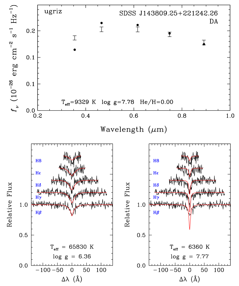
Figure 16: Top panel: Best photometric fit to SDSS J143809.25+221242.26 — a double degenerate DA+DC candidate — assuming a single DA star with a pure hydrogen atmosphere. Bottom panels: Best spectroscopic fits for the same object showing the hot (left) and cool (right) solutions.

The differences between the spectroscopic and photometric effective temperatures for the DB white dwarfs in our sample are displayed in the bottom panel of Figure 13. Overall, the photometric and spectroscopic temperatures are within the 1$\sigma$ confidence level for 69.6% of the objects in our sample, as expected from Gaussian statistics. As discussed in section 5.2, neutral broadening dominates below 16,000 K, and improvement in the treatment of van der Waals broadening is required in our models. If we exclude the objects cooler than this temperature, 71.8% of our sample is now within 1$\sigma$. Since the use of the Deridder & van Rensbergen theory rather than the Unsold theory has lowered the effective temperatures obtained with the spectroscopic technique (see top panel of Figure 12), a more refined treatment of van der Waals broadening will most likely lower those temperatures even further, giving us a better agreement between $T_{\rm spec}$ and $T_{\rm phot}$ in this regime.

We mentioned earlier that the SDSS spectroscopic data might still have a calibration issue, and that this could be the cause of the systematic offset in temperature ($T_{\rm spec}>T_{\rm phot}$) observed in Figure 13 for the DA stars. However, residual calibration problems would also affect the DB spectroscopic data. The fact that the offset in temperature is not seen in the DB sample — except for $T_{\rm spec}\lesssim 16,000$ K where we know our spectroscopic effective temperatures are more uncertain — suggests that the root of the problem most likely lies within our models, and not in the data.

Finally, the increased scatter at the high end of the temperature distribution for the DB white dwarfs in Figure 13 is again due to the lack of sensitivity of the photometric technique, and could possibly be reduced by combining multiple photometric systems.

6.2 Stellar Masses

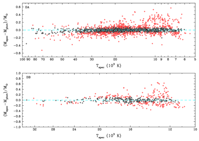
Figure 17: Differences between spectroscopic and photometric masses as a function of $T_{\rm spec}$ for the DA (top) and DB (bottom) white dwarfs in our SDSS sample. Objects with mass estimates within 1$\sigma$ are shown in black, and those outside are in red. The dashed line corresponds to $M_{\rm spec}=M_{\rm phot}$.

The differences between the spectroscopic and photometric masses — $M_{\rm spec}$ and $M_{\rm phot}$ — for the DA white dwarfs in our sample are shown as a function of $T_{\rm spec}$ in the top panel of Figure 17. Unlike for the effective temperature, the distribution of mass differences shows no obvious systematic effect, which suggests that the spectroscopic mass scale is more reliable than the corresponding temperature scale, and less affected by the problems with Stark broadening profiles discussed above.

Overall, the photometric and spectroscopic masses agree within the 1$\sigma$ confidence level for 60.9% of the objects in our sample, slightly below what is expected from Gaussian statistics. However, we can see in Figure 17 a significant number of DA stars with $M_{\rm spec}-M_{\rm phot}\gtrsim 0.2\ M_{\odot}$, which most likely correspond to unresolved DA+DA double degenerate binaries. As discussed in Section 4.3, these objects have very low inferred photometric masses, while the combined spectrum resembles that of a single DA white dwarf with intermediate effective temperature and mass (Liebert et al., 1991). An example of such a double degenerate candidate in our sample is SDSS J154130.76+032313.00, shown in Figure 18. The photometric fit indicates a very low surface gravity for this object, $\log g=7.29$, while the spectroscopic solution yields a normal value of $\log g=7.98$. Hence this system is most likely composed of two normal mass DA stars. Note that both the spectroscopic and photometric fits appear totally normal. This means that DA+DA unresolved binaries can be difficult to detect if one relies only on spectroscopic data. If we omit the binary candidates from our sample, we now find that 64% of the DA stars have photometric and spectroscopic masses that agree within 1$\sigma$, closer to what is expected from Gaussian statistics.

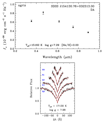
Figure 18: Best photometric (top) and spectroscopic (bottom) fits to SDSS J154130.76+032313.00, a DA+DA double degenerate candidate.

The mass comparison for the DB white dwarfs is presented in the bottom panel of Figure 17. For this sample, only half of the objects are within the 1$\sigma$ confidence level, significantly below the Gaussian statistics. However, the number of DB stars outside 1$\sigma$ is dominated by objects at low temperatures, where van der Waals broadening in our models yields uncertain spectroscopic masses. If we restrict our sample to $T_{\rm eff}>16,000$ K, the proportion of objects within 1$\sigma$ increases to 60.5%, much closer to the expectation from Gaussian statistics. The second factor that could improve the agreement between spectroscopic and photometric masses is the use of 3D hydrodynamical models, which are expected to affect the masses mostly between 20,000 K and 16,000 K, as discussed in Section 5.3. However, we note in Figure 17 that our mass estimates already agree fairly well in this particular range of temperature, suggesting that 3D effects must be small.

As for DA white dwarfs, our DB sample is likely to contain unresolved double degenerate binaries, an example of which is the DBA white dwarf SDSS J150506.24+383017.39, displayed in Figure 19. The photometric fit indicates an extremely low surface gravity of $\log g=7.37$, or a mass of 0.302 $M_{\odot}$. Also, our spectroscopic fit for the same object, under the assumption of a single star, reproduces the hydrogen lines very poorly (middle panel of Figure 19). However, if we attempt to fit the same spectrum as a combination of a DB and a DA white dwarf (here we assume $\log g=8.0$ for both components for simplicity), we are able to reproduce both the hydrogen and helium lines perfectly, as shown in the bottom panel of Figure 19.

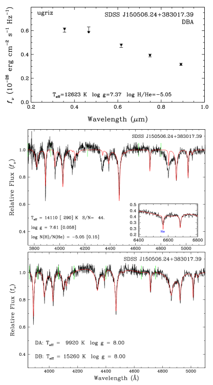
Figure 19: Top panel: Best photometric fit to the DBA white dwarf SDSS J150506.24+383017.39. Middle panel: Best spectroscopic fit of the same white dwarf under the assumption of a single star. Bottom panel: same as middle panel, but by assuming a DB+DA double degenerate binary.

The DB white dwarf SDSS J064452.30+371144.30 is another example. Its photometric fit, shown in the top panel of Figure 20, indicates a surface gravity of $\log g=7.66$, or a mass of $M=0.412~{}M_{\odot}$. In this case, however, we are able to successfully reproduce the optical spectrum with single star models, as shown in the bottom panel of Figure 20. Furthermore, the spectroscopic surface gravity has a normal value of $\log g=7.96$. This suggests that this object is an unresolved double degenerate binary composed of two DB stars with more normal masses, where the combined spectrum resembles that of a single DB white dwarf with intermediate atmospheric parameters. The deconvolution of this system will be presented elsewhere.

Bergeron et al. (2011, see also ) found no evidence for the existence of low-mass ($M<0.5\ M_{\odot}$) DB white dwarfs in their sample, suggesting that common envelope scenarios, which are often invoked to explain low-mass DA white dwarfs, are not producing DB stars. If we exclude all double degenerate binary candidates from our DB sample, as well as all cool DB white dwarfs for which spectroscopic masses are unreliable due our improper treatment of van der Waals broadening, we find no evidence for low-mass DB white dwarfs, in agreement with the conclusions of previous investigations.

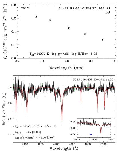
Figure 20: Best photometric (top) and spectroscopic (bottom) fits to SDSS J064452.30+371144.30, an unresolved DB+DB double degenerate candidate.

To end our mass comparison, we present in Figure 21 the cumulative photometric and spectroscopic mass distributions for both the DA and DB white dwarfs in our sample. For the DA stars, the photometric and spectroscopic distributions are in excellent agreement, in particular the mean mass values, $\langle M_{\rm phot}\rangle=0.617~{}M_{\odot}$ and $\langle M_{\rm spec}\rangle=0.615~{}M_{\odot}$. These values are entirely consistent with previous spectroscopic studies, for instance Liebert et al. (2005) using the PG sample ($\langle M\rangle=0.603~{}M_{\odot}$), Tremblay et al. (2011) using DA white dwarfs from the SDSS DR4 ($\langle M\rangle=0.613~{}M_{\odot}$), and Genest-Beaulieu & Bergeron (2014) using DA white dwarfs from the SDSS DR7 ($\langle M\rangle=0.609~{}M_{\odot}$). The dispersion of the photometric distribution ($\sigma_{\rm phot}=0.147~{}M_{\odot}$) is somewhat larger than that of the spectroscopic distribution ($\sigma_{\rm spec}=0.125~{}M_{\odot}$), which is caused by the presence of unresolved double degenerates in our sample. These objects form the small bump at $\sim 0.4~{}M_{\odot}$, and affect the photometric masses more significantly.

In the case of DB stars, the photometric and spectroscopic mass distributions have very different shapes (right panel of Figure 21) despite the fact that the mean masses, $\langle M_{\rm phot}\rangle=0.620~{}M_{\odot}$ and $\langle M_{\rm spec}\rangle=0.625~{}M_{\odot}$, are in excellent agreement. In particular, the spectroscopic distribution shows both a low-mass and a high-mass tails that are not observed in the photometric distribution. An examination of Figure 8 (bottom panel) reveals that all spectroscopic low-mass and high-mass DB stars in our sample are at low temperatures, $T_{\rm eff}<16,000~{}{\rm K}$, where the treatment of van der Waals broadening is problematic. Hence both tails are simple artifacts due to unreliable spectroscopic masses. As discussed above, we find no evidence for low-mass DB stars in the photometric mass distribution, with the exception of a small bump around 0.3 $M_{\odot}$ caused by the unresolved double degenerates in our sample.

Other mean mass values for DB white dwarfs, determined from spectroscopy, are reported in the literature — $\langle M\rangle=0.596~{}M_{\odot}$ (Voss et al., 2007, based on SPY spectra) and $0.671~{}M_{\odot}$ (Bergeron et al., 2011). Similarly, Koester & Kepler (2015) obtained a mean mass of $0.706~{}M_{\odot}$ for their complete sample of DB stars from the SDSS DR10 and 12, but a lower value of $\langle M\rangle=0.606~{}M_{\odot}$ when their sample was restricted to $16,000~{}{\rm K}\leq T_{\rm eff}\leq 22,000~{}{\rm K}$. Note that these mean mass values cannot be compared easily because of differences in the treatment of van der Waals broadening in the models, and even in the assumed convective efficiency.

Finally, we note that the mean masses for white dwarfs in the SDSS obtained by Tremblay et al. (2019, see their Figure 13, right panel) based on Gaia photometry — $\langle M\rangle=0.586~{}M_{\odot}$ and $0.580~{}M_{\odot}$ for DA and DB stars, respectively — are 0.03 to $0.04~{}M_{\odot}$ smaller than our own photometric masses based on $ugriz$ photometry. We will explore these differences in a future publication.

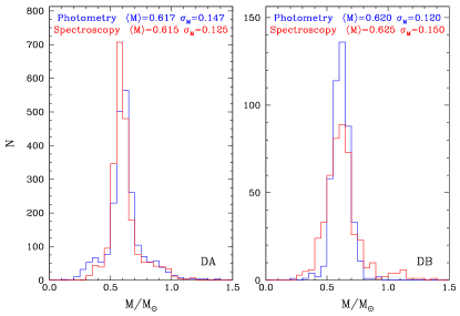
Figure 21: Photometric (blue) and spectroscopic (red) cumulative mass distributions for the DA (left) and DB (right) white dwarfs in our sample. The corresponding mean masses and dispersions are given in each panel.

7 The Mass-Radius Relation for White Dwarfs

The photometric technique allows us to measure the effective temperature $T_{\rm eff}$ and the solid angle $\pi(R/D)^{2}$, and thus the stellar radius $R$ if the distance $D$ is known from trigonometric parallax measurements. The spectroscopic technique, on the other hand, yields $T_{\rm eff}$, $\log g$, and the hydrogen abundance (or limits) in the case of DB white dwarfs. In both cases, however, the mass of the object can only be obtained from the theoretical mass-radius relation for white dwarfs, which we put to the test in this section using the results obtained so far.

Since we have trigonometric parallax measurements, we know the precise distance to every white dwarf in our sample. We can thus compare this parallactic distance $D_{\pi}$ to the distance obtained from the mass-radius relation, $D_{\rm MR}$, calculated using the procedure outlined in Bédard et al. (2017). First, the spectroscopic $\log g$ value is converted into radius $R$ using evolutionary models, which is then combined with the photometric solid angle $\pi(R/D)^{2}$ to obtain the desired distance $D_{\rm MR}$. When using this approach, the solid angle $\pi(R/D)^{2}$ can be measured in two different ways. The first one is to consider both the effective temperature and the solid angle free parameters in the minimization procedure; the second is to force the effective temperature to the spectroscopic value and to fit only the solid angle. Given the uncertainties with the spectroscopic temperature scales discussed in Section 6, we adopt the former approach. Also, it is justified to rely on spectroscopic $\log g$ values for this exercise since the surface gravity (or mass) scale appears reasonably accurate according to the results shown in Figure 17.

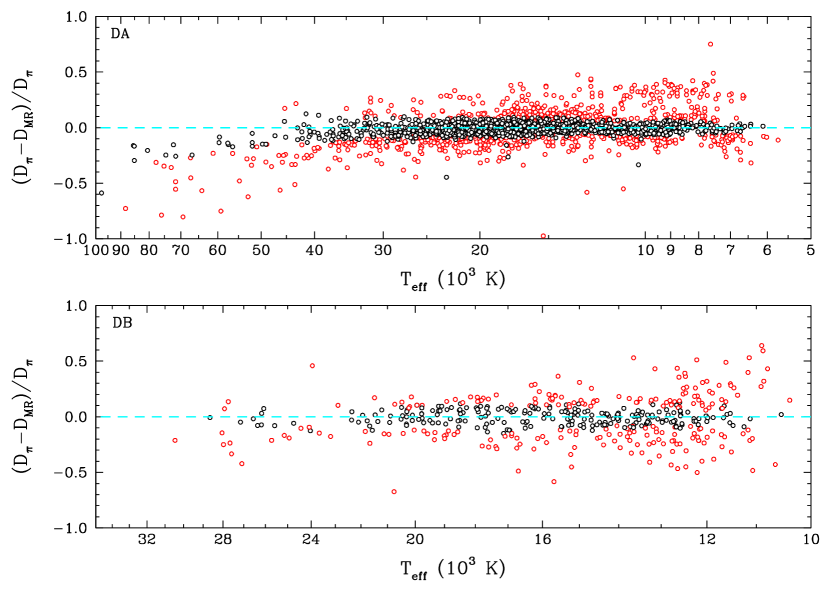
Figure 22: Comparison between the parallactic distance $D_{\pi}$ and the distance obtained from the mass-radius relation $D_{\rm MR}$, as a function of effective temperature, for both the DA (top) and DB (bottom) white dwarfs in our sample. The objects for which the distance estimates are within the 1$\sigma$ confidence level are shown in black.

Figure 22 shows the difference between $D_{\pi}$ and $D_{\rm MR}$ as a function of effective temperature, for both the DA and DB white dwarfs in our sample. For the DA stars, these distance estimates are within the 1$\sigma$ confidence level for $61.4\%$ of the objects in our sample, a value somewhat lower than what is expected from Gaussian statistics. However, we can see from this figure that most of the outliers are found (1) at high temperatures ($T_{\rm eff}\gtrsim 40,000~{}{\rm K}$) where the energy distribution sampled by the $ugriz$ photometry is in the Rayleigh-Jeans regime, and (2) at the top of the figure where unresolved double degenerate binaries are expected. If we drop all the objects above 40,000 K, as well as all the binary candidates, the fraction of objects within 1$\sigma$ increases to $64.6\%$, again much closer to the expected value of $68\%$.

For the DB stars in Figure 22, we find only 49.2% of the objects in our sample with distance estimates that are within the 1$\sigma$ confidence level, a value significantly lower than the expected 68%. Here we see, however, that most of the outliers are located at low effective temperatures where van der Waals broadening becomes important. If we restrict our sample to $T_{\rm eff}>16,000~{}{\rm K}$, and also omit the double degenerate binary candidates, the fraction of objects within 1$\sigma$ increases to $58.5\%$. This is still short of the expected fraction, but the number of objects left in our sample if we exclude the cool DB stars is admittedly small.

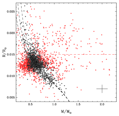
Figure 23: Radius as a function of mass for all the DA (circles) and DB (triangles) white dwarfs in our sample. The cross in the lower right corner represents the average uncertainties. Objects for which the difference between $D_{\pi}$ and $D_{\rm MR}$ exceeds the 1$\sigma$ confidence level are shown in red. Also shown are the theoretical mass-radius relations for C/O-core, thick hydrogen envelope models at $T_{\rm eff}=8000$, 15,000, and 25,000 K (black dashed lines, from left to right). The dashed red horizontal line is located at $R=0.015~{}R_{\odot}$ (see text).

Another way to test the mass-radius relation is to plot the stellar radius $R$, obtained directly from the photometric technique, against the mass obtained by combining this photometric radius with the spectroscopic $\log g$ ($g=GM/R^{2}$). This procedure allows us to measure the radius and the mass of an object without the use of any theoretical mass-radius relation. Our results for all the DA and DB white dwarfs in our sample are displayed in Figure 23, together with theoretical mass-radius relations (see Section 4.1) for C/O-core, thick hydrogen envelope models at various representative $T_{\rm eff}$ values. Note that in such a diagram, thin layer models would be almost impossible to distinguish from thick layer models (see Bédard et al. 2017). As in Bédard et al., we use different color symbols to indicate objects that exhibit differences larger than the 1$\sigma$ confidence level between the two distance estimates $D_{\pi}$ and $D_{\rm MR}$ introduced above.

While most of the data points (the black symbols) align well on the expected mass-radius relation, we see a very large scatter, especially towards higher masses. As discussed in Bédard et al. (2017), the upper right corner of this diagram is populated by unresolved double degenerate binaries. For such overluminous systems, the stellar radius is overestimated, while the spectroscopic $\log g$ value appears normal, resulting into a large inferred mass in the mass-radius diagram. For example, for the DA+DA binary candidate SDSS J154130.76+032313.00 displayed in Figure 18, we obtain from the photometric technique $R=0.02093~{}R_{\odot}$ and a spectroscopic value of $\log g_{\rm spec}=7.98$, resulting in a large mass of $M=1.513~{}M_{\odot}$, well above the Chandrasekhar limit.

Single star evolution predicts that white dwarfs with masses below $M\sim 0.45\ M_{\odot}$ should not have formed within the lifetime of the Galaxy. This corresponds to a stellar radius of $\sim$0.015 $R_{\odot}$ at 10,000 K, represented by the horizontal dashed line in Figure 23. We see that the most massive objects below this line — with normal photometric radii around 0.012 $R_{\odot}$ — are DB white dwarfs. More specifically, these correspond to the cool DB stars in our sample with $T_{\rm eff}<16,000~{}{\rm K}$, and with uncertain high $\log g$ values (see bottom panel of Figure 11). Similarly, we see a large concentration of low-mass DB white dwarfs (red triangles) on the extreme left around 0.012 $R_{\odot}$. These correspond to DB stars in the same temperature range, but this time with low spectroscopic $\log g$ values (see again bottom panel of Figure 11). All of these cool DB white dwarfs are expected to align on the mass-radius relation once a proper treatment of van der Waals broadening becomes available.

If we remove the DB stars from our sample, we are still left with a fairly large number of DA stars to the left of the theoretical curves with discrepant ($>$1$\sigma$) distance estimates (red circles). Provencal et al. (1998) proposed that these white dwarfs might not have a C/O core, but rather an iron core. Bédard et al. (2017) tested this hypothesis and found that Fe-core models could indeed explain the location of these objects in the mass-radius diagram, but they could not completely rule out that these were not normal C/O-core white dwarfs, within the uncertainties. The most compelling case of an Fe-core white dwarf was G87-7, with a parallactic distance of $D_{\pi}=15.7$ pc based on Hipparcos. The distance obtained from C/O-core models, $D_{\rm MR}=17.5$ pc, was found to be significantly different from the parallactic distance, while the distance inferred from Fe-core models, $D_{\rm MR}=15.9$ pc, was in much better agreement. This discrepancy has now been resolved with the Gaia parallax, which yields $D_{\pi}=17.07$ pc, in excellent agreement with the distance inferred from C/O-core models.

To summarize, if we restrict our analysis to single white dwarfs ($M_{\rm spec}-M_{\rm phot}<0.2\ M_{\odot})$, and to the temperature range where the physics of our model atmospheres is better understood ($T_{\rm eff}<40,000~{}{\rm K}$ for DA stars, and $T_{\rm eff}>16,000~{}{\rm K}$ for DB stars), we find that about 65% are within the 1$\sigma$ confidence level of the mass-radius relation (based on the distance comparison), and about 92% are within 2$\sigma$. We stress again the fact that we are probably underestimating in our analysis the uncertainties associated with the spectroscopic atmospheric parameters, thus these numbers represent only lower limits. With these caveats in mind, we conclude that the theoretical mass-radius relation for white dwarfs rests on solid empirical grounds, a conclusion also reached by Holberg et al. (2012), Tremblay et al. (2017), Parsons et al. (2017), and Bédard et al. (2017), but for significantly smaller samples.

8 Conclusion

We performed a detailed spectroscopic and photometric analysis of 2236 DA and 461 DB white dwarfs from the Sloan Digital Sky Survey with trigonometric parallax measurements available from the Gaia mission. The temperature and mass scales obtained from fits to $ugriz$ photometry appear reasonable for both DA and DB stars. The photometric mass distributions for DA and DB stars are comparable, with almost identical mean masses of $\langle M\rangle=0.617~{}M_{\odot}$ and $0.620~{}M_{\odot}$, respectively. However, the DA mass distribution shows well-defined low-mass and high-mass tails, which are not observed in the DB photometric mass distribution. In particular, we find no evidence in our sample for single, low-mass DB white dwarfs.

The comparison of the effective temperatures and stellar masses obtained from the photometric and spectroscopic techniques reveals several problems with the model spectra for both pure hydrogen and pure helium compositions. For DA stars, we found a systematic offset in temperature, with the spectroscopic temperatures exceeding the photometric values by $\sim$10% above 14,000 K. Since this offset is not observed for DB stars in the same temperature range, we believe that some inaccuracy in the theory of Stark broadening for hydrogen lines is at the origin of the observed temperature discrepancies. Despite these problems, the $\log g$ and mass scales derived from spectroscopy appear unaffected since the spectroscopic mass distribution agrees extremely well with that obtained from photometry. For instance, the spectroscopic mean mass for the DA stars, $\langle M\rangle=0.615~{}M_{\odot}$, differs from the photometric mean value by only $0.002~{}M_{\odot}$.

For the DB white dwarfs, both the temperature and mass scales agree well above 16,000 K, but abnormally low and high spectroscopic masses are found at lower temperatures that are significantly different from the corresponding photometric masses. We attribute these discrepancies to the inaccurate treatment of van der Waals broadening in our model spectra for DB white dwarfs, as well as to the limitations of the spectroscopic technique at low effective temperatures, when the neutral helium lines become too weak. Despite these problems, the spectroscopic mean mass for the DB stars, $\langle M\rangle=0.625~{}M_{\odot}$, differs by only $0.005~{}M_{\odot}$ from the photometric mean value.

By comparing the physical parameters using both the photometric and spectroscopic techniques, we were able to identify very easily several unresolved double degenerate binaries in our sample with various spectral types, including DA+DA, DB+DB, DA+DB, and even DA+DC systems. All of these appear overluminous, and thus have extremely low photometric masses. Double degenerates composed of identical spectral types may have normal spectroscopic $\log g$ values, however.

We finally took advantage of the Gaia parallaxes to test the theoretical mass-radius relation for white dwarfs. If we exclude the double degenerate binary candidates from our sample, and restrict our analysis to the temperature range where the spectroscopic $\log g$ values are reasonably accurate, we find that the parallactic distance and the distance obtained from the mass-radius relation are within the 1$\sigma$ confidence level for about 65% of the white dwarfs in our sample, which confirms the validity of the theoretical mass-radius relation for white dwarfs.

References

- Ali & Griem (1965) Ali, A. W., & Griem, H. R. 1965, Phys. Rev., 140, A1044
- Beauchamp (1995) Beauchamp, A. 1995, PhD thesis, Université de Montréal
- Beauchamp et al. (1996) Beauchamp, A., Wesemael, F., Bergeron, P., Liebert, J., & Saffer, R. A. 1996, in Astronomical Society of the Pacific Conference Series, Vol. 96, Hydrogen Deficient Stars, ed. C. S. Jeffery & U. Heber, 295
- Bédard et al. (2017) Bédard, A., Bergeron, P., & Fontaine, G. 2017, ApJ, 848, 11
- Bergeron et al. (2001) Bergeron, P., Leggett, S. K., & Ruiz, M. T. 2001, ApJS, 133, 413
- Bergeron et al. (1997) Bergeron, P., Ruiz, M. T., & Leggett, S. K. 1997, ApJS, 108, 339
- Bergeron et al. (1992) Bergeron, P., Saffer, R. A., & Liebert, J. 1992, ApJ, 394, 228
- Bergeron et al. (1995) Bergeron, P., Wesemael, F., Lamontagne, R., et al. 1995, ApJ, 449, 258
- Bergeron et al. (2011) Bergeron, P., Wesemael, F., Dufour, P., et al. 2011, ApJ, 737, 28
- Cukanovaite et al. (2018) Cukanovaite, E., Tremblay, P. E., Freytag, B., Ludwig, H. G., & Bergeron, P. 2018, MNRAS, 481, 1522
- Deridder & van Rensbergen (1976) Deridder, G., & van Rensbergen, W. 1976, A&AS, 23, 147
- Dufour et al. (2005) Dufour, P., Bergeron, P., & Fontaine, G. 2005, ApJ, 627, 404
- Dufour et al. (2017) Dufour, P., Blouin, S., Coutu, S., et al. 2017, in Astronomical Society of the Pacific Conference Series, Vol. 509, 20th European White Dwarf Workshop, ed. P.-E. Tremblay, B. Gaensicke, & T. Marsh, 3
- Eisenstein et al. (2006) Eisenstein, D. J., Liebert, J., Koester, D., et al. 2006, AJ, 132, 676
- El-Badry et al. (2018) El-Badry, K., Rix, H.-W., & Weisz, D. R. 2018, ApJ, 860, L17
- Fontaine et al. (2001) Fontaine, G., Brassard, P., & Bergeron, P. 2001, PASP, 113, 409
- Gaia Collaboration et al. (2018) Gaia Collaboration, Brown, A. G. A., Vallenari, A., et al. 2018, A&A, 616, A1
- Genest-Beaulieu & Bergeron (2014) Genest-Beaulieu, C., & Bergeron, P. 2014, ApJ, 796, 128
- Gentile Fusillo et al. (2019) Gentile Fusillo, N. P., Tremblay, P.-E., Gänsicke, B. T., et al. 2019, MNRAS, 482, 4570
- Gianninas et al. (2011) Gianninas, A., Bergeron, P., & Ruiz, M. T. 2011, ApJ, 743, 138
- Gomez et al. (2017) Gomez, T. A., Montgomery, M. H., Nagayama, T., Kilcrease, D. P., & Winget, D. E. 2017, in Astronomical Society of the Pacific Conference Series, Vol. 509, 20th European White Dwarf Workshop, ed. P.-E. Tremblay, B. Gaensicke, & T. Marsh, 143
- Harris et al. (2006) Harris, H. C., Munn, J. A., Kilic, M., et al. 2006, AJ, 131, 571
- Holberg et al. (2012) Holberg, J. B., Oswalt, T. D., & Barstow, M. A. 2012, AJ, 143, 68
- Hubeny & Lanz (1995) Hubeny, I., & Lanz, T. 1995, ApJ, 439, 875
- Iben (1990) Iben, Jr., I. 1990, ApJ, 353, 215
- Kepler et al. (2015a) Kepler, S. O., Pelisoli, I., Koester, D., et al. 2015a, VizieR Online Data Catalog, 744
- Kepler et al. (2015b) —. 2015b, MNRAS, 446, 4078
- Kilic et al. (2018) Kilic, M., Hambly, N. C., Bergeron, P., Genest-Beaulieu, C., & Rowell, N. 2018, MNRAS, 479, L113
- Kleinman et al. (2013) Kleinman, S. J., Kepler, S. O., Koester, D., et al. 2013, ApJS, 204, 5
- Koester & Kepler (2015) Koester, D., & Kepler, S. O. 2015, A&A, 583, A86
- Koester et al. (2009a) Koester, D., Kepler, S. O., Kleinman, S. J., & Nitta, A. 2009a, in Journal of Physics Conference Series, Vol. 172, 012006
- Koester et al. (2009b) Koester, D., Voss, B., Napiwotzki, R., et al. 2009b, A&A, 505, 441
- Lemke (1997) Lemke, M. 1997, A&AS, 122, 285
- Leo et al. (1995) Leo, P. J., Peach, G., & Whittingham, I. B. 1995, Journal of Physics B: Atomic, Molecular and Optical Physics, 28, 591
- Lewis (1967) Lewis, E. L. 1967, in Proc. Phys. Soc., Vol. 92, 817
- Liebert et al. (2005) Liebert, J., Bergeron, P., & Holberg, J. B. 2005, ApJS, 156, 47
- Liebert et al. (1991) Liebert, J., Bergeron, P., & Saffer, R. A. 1991, in NATO Advanced Science Institutes (ASI) Series C, Vol. 336, NATO Advanced Science Institutes (ASI) Series C, ed. G. Vauclair & E. Sion, 409
- Mullamphy et al. (1991) Mullamphy, D. F. T., Peach, G., & Whittingham, I. B. 1991, Journal of Physics B: Atomic, Molecular and Optical Physics, 24, 3709
- Parsons et al. (2017) Parsons, S. G., Gänsicke, B. T., Marsh, T. R., et al. 2017, MNRAS, 470, 4473
- Press et al. (1986) Press, W. H., Flannery, B. P., & Teukolsky, S. A. 1986, Numerical recipes. The art of scientific computing (Cambridge: University Press)
- Provencal et al. (1998) Provencal, J. L., Shipman, H. L., Høg, E., & Thejll, P. 1998, ApJ, 494, 759
- Rolland et al. (2018) Rolland, B., Bergeron, P., & Fontaine, G. 2018, ApJ, 857, 56
- Schlafly & Finkbeiner (2011) Schlafly, E. F., & Finkbeiner, D. P. 2011, ApJ, 737, 103
- Tremblay & Bergeron (2009) Tremblay, P.-E., & Bergeron, P. 2009, ApJ, 696, 1755
- Tremblay et al. (2011) Tremblay, P.-E., Bergeron, P., & Gianninas, A. 2011, ApJ, 730, 128
- Tremblay et al. (2019) Tremblay, P. E., Cukanovaite, E., Gentile Fusillo, N. P., Cunningham, T., & Hollands, M. A. 2019, MNRAS, 482, 5222
- Tremblay et al. (2013) Tremblay, P.-E., Ludwig, H.-G., Steffen, M., & Freytag, B. 2013, A&A, 552, A13
- Tremblay et al. (2017) Tremblay, P.-E., Gentile-Fusillo, N., Raddi, R., et al. 2017, MNRAS, 465, 2849
- Unsold (1955) Unsold, A. 1955, Physik der Sternatmospharen, MIT besonderer Berucksichtigung der Sonne., Vol. 2 (Springer)
- Voss et al. (2007) Voss, B., Koester, D., Napiwotzki, R., Christlieb, N., & Reimers, D. 2007, A&A, 470, 1079