ALIS: An efficient method to compute high spectral resolution polarized solar radiances using the Monte Carlo approach

Abstract

An efficient method to compute accurate polarized solar radiance spectra using the (three-dimensional) Monte Carlo model MYSTIC has been developed. Such high resolution spectra are measured by various satellite instruments for remote sensing of atmospheric trace gases. ALIS (Absorption Lines Importance Sampling) allows the calculation of spectra by tracing photons at only one wavelength: In order to take into account the spectral dependence of the absorption coefficient a spectral absorption weight is calculated for each photon path. At each scattering event the local estimate method is combined with an importance sampling method to take into account the spectral dependence of the scattering coefficient. Since each wavelength grid point is computed based on the same set of random photon paths, the statistical error is the almost same for all wavelengths and hence the simulated spectrum is not noisy. The statistical error mainly results in a small relative deviation which is independent of wavelength and can be neglected for those remote sensing applications where differential absorption features are of interest.

Two example applications are presented: The simulation of shortwave-infrared polarized spectra as measured by GOSAT from which CO₂ is retrieved, and the simulation of the differential optical thickness in the visible spectral range which is derived from SCIAMACHY measurements to retrieve NO₂. The computational speed of ALIS (for one- or three-dimensional atmospheres) is of the order of or even faster than that of one-dimensional discrete ordinate methods, in particular when polarization is considered.

1 Introduction

Monitoring of atmospheric trace gases is important to understand atmospheric composition and global climate change. In particular climate models require information about the concentration and global distribution of trace gases like e.g. H₂O, CO₂, O₃, or CH₄. The trace gases can be observed by measuring solar radiation which is scattered and absorbed by the molecules. Several instruments have been developed: satellite instruments provide global observations, local measurements can be taken from the ground, from air-plane, or from a balloon. Most instruments designed for trace gas concentrations observations measure radiance spectra with high spectral resolution. In the UV-Vis spectral range, absorption of radiation is due to molecular transitions; at the same time vibrational and rotational transitions can take place, which results in band spectra where the individual absorption lines can not be distinguished. Nevertheless each molecule type has its specific absorption features so that the measured spectra include information about the various trace gas concentrations. In the near-infrared spectral range there are mainly vibrational transitions; here individual lines can be identified and used for trace gas measurements.

Examples for currently operating satellite instruments that measure high resolution radiance spectra of scattered solar radiation are SCIAMACHY on the ENVISAT satellite (Gottwald et al. [1]), OMI on AURA (Levelt et al. [2]), GOME-2 on METOP (Callies et al. [3]) and TANSO-FTS on GOSAT (Kuze et al. [4]). SCIAMACHY and TANSO-FTS have the advantage of measuring not only the radiance but also the polarization state of the radiation. While extraterrestrial solar radiation is unpolarized, the radiance arriving at the satellite is polarized due to scattering by molecules, aerosols, or clouds and due to surface reflection. The polarization information may therefore be used to reduce the uncertainties in trace gas retrievals introduced by aerosols, clouds and surface reflection.

The retrieval of trace gas concentrations from radiance spectra requires a so called forward model, which can simulate such measurements for given realistic atmospheric conditions. For the often used optimal estimate retrieval method (Rodgers [5]) it is important that the forward model is fast because it has to be run several times until iteratively the atmospheric composition is found which best matches the measured spectra.

A commonly used method to simulate solar radiative transfer is the discrete ordinate method which was first described by Chandrasekhar [6] and which has been implemented for instance into the freely available well known software DISORT (Stamnes et al. [7]). The DISORT code however has the limitations that it assumes a plane-parallel atmosphere (i.e. horizontal inhomogeneities can not be taken into account) and that it neglects polarization. Polarization has been included in the VDISORT code (Schulz et al. [8]). The SCIATRAN code (Rozanov et al. [9]) is also based on the discrete ordinate method. It can optionally take into account spherical geometry as well as polarization (Rozanov and Kokhanovsky [10]).

Another method for the simulation of solar radiative transfer is the Monte Carlo method (Marchuk et al. [11], Marshak and Davis [12]), which is usually much slower than the discrete ordinate method. For this reason Monte Carlo methods have mostly been used for simulations including inhomogeneous clouds (e.g. Zinner et al. [13]) for which the plane-parallel approximation can not be applied. We have developed a new Monte Carlo method which calculates high spectral resolution radiance spectra very efficiently. The algorithm, named ALIS (Absorption Lines Importance Sampling), does not require any approximations, in particular it can easily take into account polarization and horizontal inhomogeneity. We show that the computational time of ALIS for high resolution radiance spectra is comparable to or even faster than the discrete ordinate approach, especially if polarization is included. This means that the algorithm is sufficiently fast to be used as forward model for trace gas retrieval algorithms. The basis of the ALIS method is that all wavelengths are calculated at the same time based on the same random numbers. This method which is sometimes called “method of dependent sampling” (Marchuk et al. [11]) has been used for various applications, e.g. to calculate mean radiation fluxes in the near-IR spectral range (Titov et al. [14]), to compute multiple-scattering of polarized radiation in circumstellar dust shells (Voshchinnikov and Karjukin [15]), or to calculate Jacobians (Deutschmann et al. [16]). We have validated ALIS by comparison to the well-known and well-tested DISORT program, originally developed and implemented by Stamnes et al. [7] in FORTRAN77. We use a new version of the code implemented in C (Buras et al. [17]) with increased efficiency and numerical accuracy.

2 Methodology

The new method Absorption Lines Importance Sampling (ALIS), which allows fast calculations of spectra in high spectral resolution, has been implemented into the radiative transfer model MYSTIC (Monte Carlo code for the phYsically correct Tracing of photons In Cloudy atmospheres; Mayer [18]). MYSTIC is operated as one of several solvers of the libRadtran radiative transfer package (Mayer and Kylling [19]). The common model geometry of MYSTIC is a 3D plane-parallel atmosphere to simulate radiances or irradiances in inhomogeneous cloudy conditions. The model can also be operated in 1D spherical model geometry (Emde and Mayer [20]) which makes it suitable also for limb sounding applications. Recently MYSTIC has been extended to handle polarization due to scattering by randomly oriented particles, i.e. clouds, aerosols, and molecules (Emde et al. [21]), and to handle topography (Mayer et al. [22]). Several variance reduction techniques were also introduced to MYSTIC in order to speed up the computation of radiances in the presence of clouds and aerosols (Buras and Mayer [23]).

2.1 Monte Carlo method for solar atmospheric radiative transfer

This section briefly describes the implementation of solar radiative transfer in MYSTIC which is explained in detail in Mayer [18]. We describe only those details which are required to understand the following sections about the ALIS method.

In the forward tracing mode “photons” are traced on their way through the atmosphere. The photons are generated at the top of the atmosphere where their initial direction is given by the solar zenith angle and the solar azimuth angle.

Absorption and scattering are treated separately: Absorption is considered by a photon weight according to Lambert-Beer’s law:

$$w_{\rm abs}=\exp\left(-\int_{0}^{s}\beta_{\rm abs}(s^{\prime}){\rm d}s^{\prime}\right)$$ (1)

Here ${\rm d}s^{\prime}$ is a path element of the photon path and $\beta_{\rm abs}=\sum_{i=1}^{N}{\beta_{\rm abs,i}}$ is the total absorption coefficient which is the sum of the $N$ individual absorption coefficients $\beta_{\rm abs,i}$ of molecules, aerosols, water droplets, and ice crystals. The integration is performed over the full photon path.

The free path of a photon until a scattering interaction takes place is sampled according to the probability density function (PDF):

$$P(s)=\beta_{\rm sca}(s)\exp\left({-\int_{0}^{s}\beta_{\rm sca}(s^{\prime}){\rm d}s^{\prime}}\right)$$ (2)

Here $\beta_{\rm sca}=\sum_{i=1}^{N}{\beta_{\rm sca,i}}$ is the total scattering coefficient of $N$ interacting particle and molecule types.

We use a random number $r\in[0,1]$ to decide which interaction takes place. If there are $N$ types of particles and molecules at the place of scattering, the photon interacts with the $j^{th}$ type if the random number fulfills the following condition:

$$\frac{\sum_{i=1}^{j-1}\beta_{\rm sca,i}}{\beta_{\rm sca}}<r\leq\frac{\sum_{i=1}^{j}\beta_{\rm sca,i}}{\beta_{\rm sca}}$$ (3)

At each scattering event the “local estimate” weight is calculated which corresponds to the probability that the photon is scattered into the direction of the detector and reaches it without further interactions:

$$w_{{\rm le},is}=\frac{P_{\rm 11}(\theta_{p})\exp\left(-\int{(\beta_{\rm abs}+\beta_{\rm sca}){\rm d}s^{\prime}}\right)}{\cos(\theta_{d})}$$ (4)

Here $\theta_{p}$ is the angle between photon direction (before scattering) and the radiance direction. The phase function P₁₁ (first element of the scattering matrix) gives the probability that the photon is scattered into the direction of the detector, “$is$” denotes the scattering order. In order to calculate the probability that the photon actually reaches the detector the Lambert-Beer term for extinction $\exp\left(-\int{(\beta_{\rm abs}+\beta_{\rm sca}){\rm d}s^{\prime}}\right)$ needs to be included. Finally we have to divide by the zenith angle of the detector direction $\theta_{d}$ to account for the slant area in the definition of the radiance. The contribution of the photon to the radiance measured at the detector is then given as

$$I_{i}=\sum_{is=1}^{\rm N_{s}}w_{{\rm abs},is}w_{{\rm le},is}$$ (5)

Here $i$ is the index of the photon, $N_{s}$ is the number of scattering events along the photon path, and $w_{{\rm abs},is}$ is the absorption weight (Eq. 1) evaluated at the scattering order $is$. One can show formally that the sum over the local estimate weights corresponds to a von Neumann series which is a solution of the integral form of the radiative transfer equation (see e.g. Marshak and Davis [12]).

Additional weights are required to take into account polarization (Emde et al. [21]) and variance reduction techniques (Buras and Mayer [23]).

After tracing $N_{p}$ photons the radiance is given by the average contribution of all photons:

$$I=\frac{\sum_{1}^{N_{p}}I_{i}}{N_{p}}$$ (6)

The methods described above are implemented for monochromatic radiative transfer. If one wants to calculate a radiance spectrum using these methods one has to calculate all spectral points subsequently. Here usually a very high accuracy is required in order to distinguish spectral features from statistical noise which means that such calculations are computationally expensive.

2.2 Calculation of high spectral resolution clear-sky radiance spectra

In the following an efficient method how to compute high spectral resolution radiance spectra will be described and demonstrated on the example of the spectral region from 765–768 nm in the O₂A absorption band where we calculate the spectrum with a resolution of 0.003 nm. The line-by-line gas absorption coefficients have been computed using the ARTS model (Buehler et al. [25], Eriksson et al. [26]) for the standard mid-latitude summer atmosphere (Anderson et al. [27]). Fig. 1 shows the vertically integrated optical thickness of molecular absorption $\tau_{\rm abs,v}$ (top) and scattering $\tau_{\rm sca,v}$ (bottom). Whereas the scattering optical thickness for the cloudless, aerosol-free atmosphere is rather small and almost constant, it varies only from about 0.0239 to 0.0243, the absorption optical thickness varies over five orders of magnitude, from about 10^-3 to 10² (note the logarithmic scale).

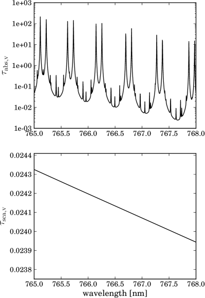
Figure 1: Integrated vertical optical thickness of molecular absorption (top) and molecular scattering (bottom).

As mentioned in the previous section, absorption is considered separately by calculating the absorption weight $w_{\rm abs}$ (Eq. 1). In order to calculate a radiance spectrum taking into account the spectral variation of the absorption coefficient $\beta_{\rm abs}$ we can easily calculate the absorption weight for each wavelength and get a spectrally dependent absorption weight vector:

$$w_{\rm abs}(\lambda)=\exp\left(-\int_{0}^{s}\beta_{\rm abs}(\lambda,s^{\prime}){\rm d}s^{\prime}\right)$$ (7)

Here $\lambda$ denotes the wavelength of the radiation. In practice the integral corresponding to the absorption optical thickness $\tau_{\rm abs}=\int_{0}^{s}\beta_{\rm abs}{\rm d}s^{\prime}$ is calculated step by step while the photon moves through the layers/boxes of the discretized model atmosphere (see Mayer [18]):

$$\tau_{\rm abs}(\lambda)=\sum_{p}{\beta_{\rm abs}(\lambda,p){\rm\Delta s}_{p}}$$ (8)

Here the $p$ denotes the step index along the photon path, and ${\rm\Delta s}_{p}$ is the pathlength of step $p$. We also include the spectrally dependent absorption coefficient $\beta_{\rm abs}(\lambda)$ in the local estimate weight $w_{{\rm le},is}(\lambda)$. Thus we only need to trace the photons for one wavelength, calculate the spectral absorption weights and get the full radiances spectrum with high spectral resolution. For each photon we get (compare Eq. 5):

$$I_{i}(\lambda)=\sum_{is=1}^{\rm N_{s}}w_{{\rm abs},is}(\lambda)w_{{\rm le},is}(\lambda)$$ (9)

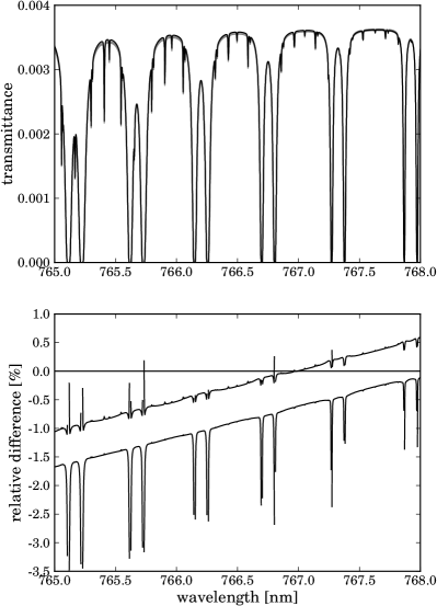
Figure 2: Radiance spectra calculated with MYSTIC in comparison to DISORT calculations. The top panel shows the transmittance (radiance normalized to extraterrestrial irradiance) spectra of two independent MYSTIC runs (grey lines) and the DISORT result (black line) and the bottom panel shows the relative differences between the MYSTIC runs and DISORT in percent.

Fig. 2 shows two spectral calculations using this method. Here we assumed that the sun is in the zenith and the sensor is on the ground and measures with a viewing angle of 60^∘. We did not include any sensor response function. The upper panel shows the transmittance spectra (radiance divided by extraterrestrial irradiance) and the lower panel shows the relative difference to the DISORT solver operated with 32 streams. The MYSTIC calculations with 10⁶ photons took 13 s on a single processor with 2 GHz CPU (all computational times in the following refer to this machine), the DISORT calculation took 25 s. The relative difference between MYSTIC and DISORT is less than about 2% with some exceptions where the transmittance is almost zero. The spectral features in the MYSTIC calculations are well resolved. The two MYSTIC runs used exactly the same setup but the results show a deviation between each other and with respect to the DISORT result. This deviation is due to the statistical error of the Monte Carlo calculation, with 10⁶ photons the standard deviation is 0.66%. Hence the deviation can be reduced by running more photons. Since the same photon paths are used to compute all wavelengths the deviation is the same at all spectral data points and the spectra are not noisy. However the deviation shows a spectral dependence which is not a statistical error but can be attributed to the spectral dependence of Rayleigh scattering which has been neglected so far. In the calculation $\beta_{\rm sca}$ was set to a constant value corresponding to $\beta_{\rm sca}$ at 766.5 nm. In the next section we will describe how to include the spectral dependence of the scattering coefficient.

2.3 Importance sampling for molecular scattering

Eq. 2 is the PDF which we use for sampling the free pathlength of the photons, where the scattering coefficient $\beta_{\rm sca}$ now becomes wavelength dependent. We want to use this PDF for sampling the pathlength for all wavelengths. In order to ensure that the results are correct for all wavelength we introduce a correction weight (importance sampling method, see e.g. Ripley [28]):

$$w_{\rm sca1}(\lambda,s)$$ (10)

$$=\frac{\beta_{\rm sca}(\lambda,s)\exp\left(-\int_{0}^{s}\beta_{\rm sca}(\lambda,s^{\prime}){\rm d}s^{\prime}\right)}{\beta_{\rm sca}(\lambda_{c},s)\exp\left(-\int_{0}^{s}\beta_{\rm sca}(\lambda_{c},s^{\prime}){\rm d}s^{\prime}\right)}$$

$$=\frac{\beta_{\rm sca}(\lambda,s)}{\beta_{\rm sca}(\lambda_{c},s)}\exp\left(-\int_{0}^{s}(\beta_{\rm sca}(\lambda,s^{\prime})-\beta_{\rm sca}(\lambda_{c},s^{\prime})){\rm d}s^{\prime}\right)$$

Here $\lambda_{c}$ ($c$ for “computational”) is the wavelength corresponding to the scattering coefficient that is used to sample the photon free path. As in the previous section we write the second part of this expression as a sum over the model layers/boxes:

$$w_{\rm sca1}(\lambda,s) =\frac{\beta_{\rm sca}(\lambda,s)}{\beta_{\rm sca}(\lambda_{c},s)}$$ (11)

$$\times\exp\left(-\sum_{p}{(\beta_{\rm sca}(\lambda,p)-\beta_{\rm sca}(\lambda_{c},p))\Delta s_{p}}\right)$$

The probability that the photon is scattered into a direction with scattering angle $\theta_{p}$ is given by the phase function $P_{11}(\lambda,\theta_{p})$. So we need another weight to correct for the spectral dependence of the phase function which can again easily be derived using the importance sampling method:

$$w_{{\rm sca2},is}(\lambda,s)=\frac{P_{11}(\lambda,\theta_{p},s)}{P_{11}(\lambda_{c},\theta_{p},s)}$$ (12)

Here $s$ is the location at which the photon is scattered. Note that in the case where we have only molecules as interacting particles and neglect depolarization $P_{11}$ is the Rayleigh phase function

$$P_{11}(\theta_{p})=\frac{3}{4}(1+\cos^{2}\theta_{p})$$ (13)

Also, as long as we neglect the wavelength dependence of the Rayleigh depolarization factor (see e.g. Hansen and Travis [29]) the Rayleigh phase function is wavelength-independent and $w_{{\rm sca2},is}(\lambda)=1$.

The final result for the contribution of a photon including the spectral dependence of absorption and scattering to the spectral radiance is:

$$I_{i}(\lambda)=$$ (14)

$$\sum_{\rm is=1}^{\rm N_{s}}w_{{\rm abs},is}(\lambda)\left(\prod_{is^{\prime}=1}^{is}w_{{\rm sca1},is^{\prime}}(\lambda,s^{\prime})w_{{\rm sca2},is^{\prime}}(\lambda,s^{\prime})\right)w_{{\rm le},is}(\lambda)$$

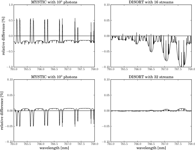
Figure 3: Relative differences of various model setups with respect to a DISORT calculation with 64 streams. The left panels show MYSTIC calculations with 10⁶ and 10⁹ photons respectively. The right panels show DISORT calculations with 16 and 32 streams respectively.

Now we calculate again the spectrum in the O₂A-band from 765–768 nm with $\lambda_{c}=$765 nm and compare the result with an accurate DISORT calculation using 64 streams. The top left panel of Fig. 3 shows the relative difference of a MYSTIC run with 10⁶ photons, which takes 14.6 s, to DISORT. We see that there is still a relative deviation of about 0.4% which is due to the statistical error of the Monte Carlo calculation, but the spectral dependence of the deviation is now removed because we have corrected the spectral dependence of the scattering coefficient. In order to check whether the method is correctly implemented without any bias (apart from the statistical error) we performed a MYSTIC run with 10⁹ photons. The result is shown in the lower left panel. The spectrally independent deviation has almost vanished ($<$0.01%) and the relative difference between MYSTIC and DISORT is below 0.05%. For comparison we show in the right panels of the figure DISORT runs with 16 and 32 streams respectively compared to the DISORT run with 64 streams. The difference between DISORT (16 streams) and DISORT (64 streams) is actually larger than the difference between MYSTIC (10⁹ photons) and DISORT (64 streams).

It should be noted that this Monte Carlo method does only work well as long as the scattering coefficient does not vary too much within the simulated wavelength region. Else the scattering weights can obtain values very far from 1, resulting in large statistical noise and slow convergence.

2.4 Calculation of high resolution spectra including aerosol and cloud scattering

It is straightforward to apply the method to an atmosphere including clouds and/or aerosols. We just need to use the total absorption and scattering coefficients

$$\beta_{\rm abs}(\lambda)=\sum_{i=1}^{N}{\beta_{\rm abs,i}}(\lambda)$$ (15)

$$\beta_{\rm sca}(\lambda)=\sum_{i=1}^{N}{\beta_{\rm sca,i}}(\lambda)$$ (16)

and the average phase function given by

$$P_{\rm 11}(\lambda)=\frac{\sum_{i=1}^{N}{\beta_{\rm sca,i}(\lambda)P_{\rm 11,i}(\lambda)}}{\beta_{\rm sca}(\lambda)}$$ (17)

Here $N$ is the number of interacting particles/molecules. These quantities can be used to compute the wavelength dependent weights $w_{\rm abs}(\lambda)$ (Eq. 7), $w_{\rm sca1}(\lambda)$ (Eq. 11) and $w_{\rm sca2}(\lambda)$ (Eq. 12). In MYSTIC we so far consider only the spectral dependence of molecular scattering because the spectral dependence of cloud and aerosol scattering can safely be neglected in narrow wavelength intervals.

3 Applications

3.1 Simulation of polarized near infrared spectra in cloudless conditions

The Greenhouse Gases Observing Satellite (GOSAT) determines the concentrations of carbon dioxide and methane globally from space. The spacecraft was launched on January 23, 2009, and has been operating properly since then. Information about the project can be found on the web-page http://www.gosat.nies.go.jp. GOSAT carries the Thermal and Near Infrared Sensor for Carbon Observation Fourier-Transform Spectrometer (TANSO-FTS) (Kuze et al. [4]) which measures in 4 spectral bands (band 1: 0.758–0.775 $\mu$m, band 2: 1.56–1.72 $\mu$m, band 3: 1.92–2.08 $\mu$m, band 4: 5.56–14.3 $\mu$m). The spectral resolution in all bands is 0.2 cm^-1. For the visible spectral range (bands 1–3) polarized observations are performed. In order to analyze this data a fast polarized radiative transfer code is required. The Monte Carlo approach which is described in this study is an alternative to commonly used discrete ordinate or doubling and adding codes. The approach is fully compatible to the implementation of polarization in MYSTIC as described in Emde et al. [21] and validated in Kokhanovsky et al. [30], because the weight vector which is calculated to take into account the polarization state of the photon does not interfere with the spectral weights. An advantage of the Monte Carlo approach is of course that it is easy to take into account horizontal inhomogeneities of clouds, aerosols, and molecules.

In the following we show an example simulation where we selected a spectral window of band 3 from 4815–4819 cm^-1 (corresponding to $\approx$2.075–2.077 $\mu$m) in the near infrared. The radiance simulation is performed with a spectral resolution of 0.01 cm^-1. The atmospheric profiles (pressure, temperature, trace gases) correspond to the standard mid-latitude summer atmosphere as defined by Anderson et al. [27]. The molecular absorption coefficients have been computed using the ARTS line-by-line model. We assume a thin maritime aerosol layer with an optical thickness of 0.05 at 2 $\mu$m. We took the refractive indices and the size distribution data from Hess et al. [31] (maritime clean aerosol mixture) and performed Mie calculations to obtain the aerosol optical properties including the phase matrix. We assume an underlying water surface which is modeled using the reflectance matrix as defined in Mishchenko and Travis [32]. The reflectance matrix is based on the Fresnel equations, on Cox and Munk [33, 34] to describe the wind-speed dependent slope of the waves, and on Tsang et al. [35] to account for shadowing effects. The wind speed was taken to be 5m/s. The viewing angle of the FTS is 30^∘ and simulations have been performed for the principal plane assuming different solar zenith angles $\theta_{0}$. The full Stokes vector has been computed for all setups.

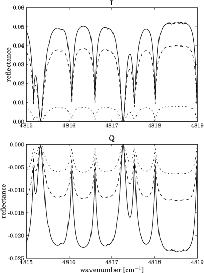
Figure 4: Simulated GOSAT spectra over ocean. The assumed wind speed is 5 m/s. The viewing angle of the FTS is 30^∘. The line-styles correspond to different solar zenith angles, the solid line corresponds to 30^∘, i.e. the sun glint is observed, the dashed and the dash-dotted lines correspond to 20^∘ and 60^∘, respectively. All simulations are in the principal plane. The upper panel shows the normalized reflected intensity $I$ and the lower panel shows the polarization difference $Q$.

Fig. 4 shows the simulated GOSAT spectra. The solid lines correspond to $\theta_{0}$=30^∘, in this case the FTS observes the center of the sun glint, therefore this spectrum shows the highest reflectance. The dashed lines are for $\theta_{0}$=20^∘, still in the sun-glint region and the dashed-dotted lines are for $\theta_{0}$=60^∘ which is not influenced much by the sun glint. The computation time for each polarized spectrum using 10⁶ photons was 2 minutes and 25 seconds, the standard deviation (approximately the same for each Stokes vector component) for $\theta_{0}$=20^∘ and $\theta_{0}$=30^∘ is 0.03%, for $\theta_{0}$=60^∘ it is 0.16%.

3.2 Simulations of differential optical thickness in broken cloud conditions

Retrievals of the tropospheric NO₂ column from SCIAMACHY data are based on the differential optical absorption spectroscopy (DOAS) method (Richter and Burrows [36], Richter et al. [37]). For this method the measured spectra are converted to so-called differential optical thicknesses defined as

$$D(\lambda)=\ln(I_{\rm TOA}(\lambda))-P_{3}(\lambda)$$ (18)

where $I_{\rm TOA}(\lambda)$ is the reflectance at the top of the atmosphere. $P_{3}(\lambda)$ is a third degree least square polynomial fit of the logarithm of $I_{\rm TOA}(\lambda)$ with respect to the wavelength, which removes the slowly varying part of the spectrum. The conversion of $I_{\rm TOA}(\lambda)$ into $D(\lambda)$ improves the contrast of the NO₂ absorption line depths and thereby the accuracy of the retrieval. The retrieval algorithm minimizes the function

$$F(\lambda,V_{\rm NO_{2},ret})=\left|D(\lambda,V_{\rm NO_{2},true})-D(\lambda,V_{\rm NO_{2},ret})\right|$$ (19)

where $V_{\rm NO_{2},true}$ and $V_{\rm NO_{2},ret}$ are the true and the retrieved tropospheric NO₂ columns, respectively.

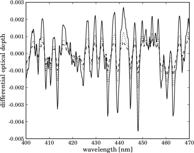
Figure 5: Differential optical thickness calculated for three different NO₂ profiles, corresponding to low (- -), medium ($\cdots$) and highly polluted (—) conditions. The spectra have been computed using MYSTIC with 10⁵ photons.

Our new method allows efficient computations of $D(\lambda)$. As an example Fig. 5 shows spectra for three different NO₂ profiles, corresponding to low, medium and highly polluted conditions. The Lambertian surface albedo was set to 0.1 and the solar zenith angle to 32^∘. NO₂ and O₃ profiles are the same as used in the study by Vidot et al. [38]. The NO₂ absorption cross sections have been taken from Burrows et al. [39], ozone absorption was also included in the simulations using the cross sections by Molina and Molina [40]. The spectral resolution of the simulation is 0.1 nm.

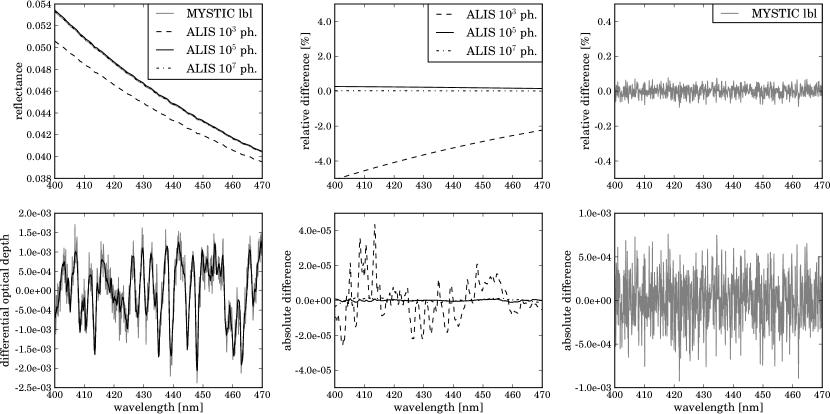
Figure 6: Simulations for NO₂ profile corresponding to medium polluted conditions. The top left panel shows the reflectance and the bottom left panel the differential optical thickness. The black lines correspond to Monte Carlo simulations using the ALIS method with different number of photons (10³, 10⁵, and 10⁷), the grey line shows a Monte Carlo simulation without ALIS (all wavelengths are calculated independently). The middle panels show differences w.r.t. DISORT for the ALIS simulations and the right plots show differences w.r.t. DISORT for the MYSTIC calculation without using ALIS.

Fig. 6 shows calculations for the NO₂ profile corresponding to medium polluted conditions. The top left panel shows the reflectance, where the grey line corresponds to a MYSTIC calculation without using ALIS, i.e. all wavelengths are simulated subsequently using 10⁷ photons for each wavelength. The standard deviation for each wavelength is about 0.03%. This calculation took 33 h 12 min on one CPU. The black line shows the calculations using ALIS with different numbers of photons. The calculation using 10³ photons took 0.9 s, the one with 10⁵ photons took 38 s, and the one with 10⁷ photons took 63 min 53 s. Obviously the absorption features of NO₂ are barely visible in the reflectance plot. There is a deviation between the simulations which is due to the statistical error of the simulation using ALIS with 10³ or 10⁵ photons. The top middle panel shows the relative differences of the ALIS simulations w.r.t. DISORT, which requires 30 s computation time with 32 streams. Obviously the relative difference decreases with increasing number of photons. The top right panel shows the relative difference between the MYSTIC calculation without ALIS and DISORT. The relative difference is less than 0.1% and shows the typical Monte Carlo noise.

The bottom left panel shows the differential optical thicknesses derived from the simulations. Here the statistical noise of the MYSTIC calculation without ALIS (grey line) is clearly visible. All ALIS simulations result in a smooth differential optical thickness because all wavelengths are calculated based on the same photon paths. This yields a relative deviation in the reflectance which is independent of wavelengths and can be removed completely by subtracting the fitted polynomial. The bottom middle panel shows the absolute difference between the differential optical thicknesses derived from the ALIS simulations and the one derived from the DISORT simulation. Even for the simulation with only 10³ photons the differential optical thickness is quite accurate, the difference w.r.t. DISORT is of the order of a few per-cent. Using 10⁵ photons or more yields very accurate differential optical thicknesses, the difference is here well below 1%. The bottom right panel shows the difference between the MYSTIC calculation without ALIS and the DISORT calculation. The difference is of the same order of magnitude as the differential optical thickness itself and hence the accuracy of this simulation would not be sufficient for NO₂ retrievals.

Fig. 6 clearly demonstrates that a common Monte Carlo approach which calculates wavelength by wavelength sequentially is extremely inefficient for simulations of the differential optical thickness because each wavelength has an independent statistical error which is larger than the absorption features unless a huge number of photons is used. In order to obtain a result with an accuracy comparable to ALIS with 10³ photons (0.9 s computation time), MYSTIC without ALIS would require at least 10⁹ photons per wavelength which would take about 138 days computation time.

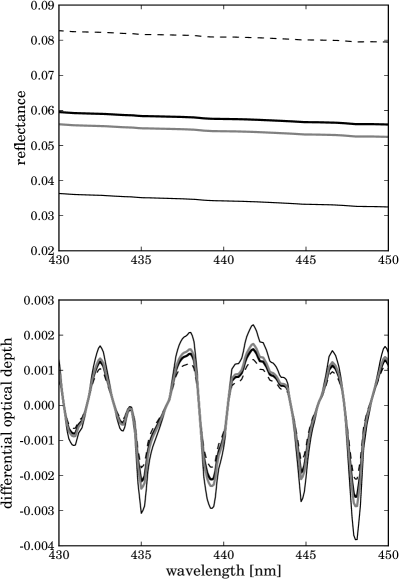
Figure 7: Impact of cirrus clouds on a spectrum used for NO₂ retrievals. The cirrus clouds are modeled as 1$\times$1$\times$1 km³ cubes, the cloud fraction in the model domain is 0.5. Black lines correspond to the independent pixel (IPA) calculation and grey lines to the 3D calculation. Upper panel: The thick lines show the reflectance $R$ of the full domain. The dashed line shows the the clear-sky pixels only ($R_{\rm clear}$) and the thin solid line shows the cloudy pixels ($R_{\rm cloud}$) for the IPA calculation. The lower panel shows corresponding differential optical thicknesses, where the lines styles are defined as above.

The impact of cirrus clouds on tropospheric NO₂ retrievals has been investigated in a sensitivity study by Vidot et al. [38]. They take into account the sub-pixel inhomogeneity by a simple independent pixel approach. Using our Monte Carlo approach we can take into account full 3-dimensional radiative transfer, e.g. the interaction between the cloudy and the clear-sky part of the domain. Fig. 7 shows an example where the setup is similar to the study by Vidot et al. [38]. We have taken a very simple 3D cloud field, the cirrus clouds were modeled as 1$\times$1$\times$1 km³ cubes and arranged as a chess-board, hence the cloud fraction $c$ is 0.5. The surface albedo is 0.05 and the solar zenith angle is 30^∘. The optical thickness of the clouds is 3, the geometrical thickness is 1 km, the cloud base height is 10 km and the effective radius is 30 $\mu$m where the parameterization by Baum et al. [41, 42] was used for the cirrus optical properties. The solar zenith angle is 30^∘ and the wavelength range is 400 nm to 470 nm. We performed 3D calculation and also used the independent pixel approximation (IPA) for comparison. All simulations shown in Fig. 7 were calculated using MYSTIC with ALIS. The reflectance for the IPA simulation is calculated as the sum of the reflectance of the clear-sky part $R_{\rm clear}$ and the reflectance of the cloudy part $R_{\rm cloud}$ weighted with the cloud fraction:

$$R=cR_{\rm cloud}+(1-c)R_{\rm clear}$$ (20)

In order to speed up the calculations in the presence of clouds, the variance reduction technique VROOM (Buras and Mayer [23]) was used. Using VROOM the simulation 10⁵ photons are sufficient to obtain an accurate result with a standard deviation of approximately 0.5%. The 3D calculation using these settings took 1 min 34 s, an IPA calculation using DISORT with 32 streams takes 58 s.

Fig. 7 shows a part of the spectrum where we have pronounced features in the differential optical depth. In the top panel one can see that for all wavelengths the reflectance in the 3D calculation is smaller than in the IPA calculation, because photons which are scattered out of the clouds on the sides have a higher probability of being transmitted to the surface.

The bottom panel of Fig. 7 shows the differential optical thickness. The difference between IPA and 3D is in this case about 10% which will cause an error of some per cent in the tropospheric NO₂ retrievals. Note that this calculation is only an example to demonstrate the new algorithm to calculate high spectral resolution spectra using the Monte Carlo method. With different setups the error on the retrieval can be completely different.

4 Conclusions

We have developed the new method ALIS (absorption lines importance sampling) that allows to compute polarized radiances in high spectral resolution using the Monte Carlo method in a very efficient way. We sample random photon paths at one wavelength. For these random paths we calculate a spectral absorption weight using the wavelength dependent absorption coefficients of the model boxes. In order to correct for the wavelength dependence of Rayleigh scattering an importance sampling method is applied. If necessary the same method can be applied to correct for the spectral dependence of cloud and aerosol scattering. The method allows us to calculate radiances for many wavelengths at the same time without significantly increasing the computational cost. ALIS has been implemented in the MYSTIC model which handles three-dimensional radiative transfer in cloudy atmospheres including polarization and complex topography.

The new algorithm ALIS has been validated by comparison to the well-known and well-tested DISORT solver. It has been shown that ALIS does not produce any bias apart from the statistical noise. Since all wavelengths are computed at once, the statistical error is the same at all wavelength which results mainly in a relative deviation which is independent of wavelength. However, for remote sensing applications, where mostly differential absorption features are of interest, this deviation does not matter.

Two example applications are shown. First the simulation of polarized near-infrared spectra over an ocean surface as measured by e.g. GOSAT. Here we simulated the Stokes vector with a standard deviation smaller than 0.05% for 400 spectral points in 2 minutes 25 seconds on a single PC. For a standard deviation of 0.5% the calculation would be 100 times faster. These short computation times show that the algorithm has the potential to be used as a forward model for trace gas retrievals from polarized radiance measurements, in particular since commonly used discrete ordinate methods become much slower when they include polarization.

The second example is the simulation of the differential optical thickness from 400 nm to 470 nm which is used to retrieve NO₂ from e.g. SCIAMACHY. Here the computation time for accurate (scalar) simulations was comparable to DISORT. We performed this calculation also for an inhomogeneous cloud scene where cirrus clouds are approximated by simple cubes. We compared the result of the 3D simulation with an independent pixel calculation and found a difference of about 10 % in the differential optical thickness for this example. The calculations show that ALIS is suitable to study effects of horizontal inhomogeneity on trace gas retrievals in presence of cirrus clouds.

References

References

- Gottwald et al. [2006] M. Gottwald, H. Bovensmann, G. Lichtenberg, S. Noel, A. von Bargen, S. Slijkhuis, A. Piters, R. Hoogeveen, C. von Savigny, M. Buchwitz, A. Kokhanovsky, A. Richter, A. Rozanov, T. Holzer-Popp, K. Bramstedt, J.-C. Lambert, J. Skupin, F. Wittrock, H. Schrijver, J. Burrows, SCIAMACHY, Monitoring the Changing Earth’s Atmosphere, DLR, 2006.
- Levelt et al. [2006] P. F. Levelt, G. H. J. van den Oord, M. R. D. adm A. Mälkki, H. Visser, J. de Vries, P. Stammes, J. Lundell, H. Saari, The Ozone Monitoring Instrument, IEEE Transactions on Geoscience and Remote Sensing 44 (5) (2006) 1093–1101.
- Callies et al. [2000] J. Callies, E. Corpaccioli, M. Eisinger, A. Hahne, A. Lefebvre, GOME-2 - Metop’s Second Generation sensor for Operational Ozone Monitoring, ESA Bulletin 102.
- Kuze et al. [2009] A. Kuze, H. Suto, M. Nakajima, T. Hamazaki, Thermal and near infrared sensor for carbon observation Fourier-transform spectrometer on the Greenhouse Gases Observing Satellite for greenhouse gases monitoring, Appl. Opt. 48 (2009) 6716–6733.
- Rodgers [2000] C. Rodgers, Inverse Methods for Atmospheric Sounding: Theory and Practice, World Scientific, 2000.
- Chandrasekhar [1950] S. Chandrasekhar, Radiative transfer, Oxford Univ. Press, UK, 1950.
- Stamnes et al. [2000] K. Stamnes, S.-C. Tsay, W. Wiscombe, I. Laszlo, DISORT, a General-Purpose Fortran Program for Discrete-Ordinate-Method Radiative Transfer in Scattering and Emitting Layered Media: Documentation of Methodology, Tech. Rep., Dept. of Physics and Engineering Physics, Stevens Institute of Technology, Hoboken, NJ 07030, 2000.
- Schulz et al. [1999] F. M. Schulz, K. Stamnes, F. Weng, VDISORT: An improved and generalized discrete ordinate method for polarized (vector) radiative transfer, J. Quant. Spectrosc. Radiat. Transfer 61 (1) (1999) 105–122.
- Rozanov et al. [2005] A. Rozanov, V. Rozanov, M. Buchwitz, A. Kokhanovsky, J. P. Burrows, SCIATRAN 2.0 A new radiative transfer model for geophysical applications in the 175–2400 nm spectral region, Adv. Space Res. 36 (2005) 1015–1019.
- Rozanov and Kokhanovsky [2006] V. V. Rozanov, A. A. Kokhanovsky, The solution of the vector radiative transfer equation using the discrete ordinates technique: Selected applications, Atmospheric Research 79 (2006) 241–265.
- Marchuk et al. [1980] G. I. Marchuk, G. A. Mikhailov, M. A. Nazaraliev, The Monte Carlo methods in atmospheric optics, Springer Series in Optical Sciences, Berlin: Springer, 1980.
- Marshak and Davis [2005] A. Marshak, A. Davis, 3D Radiative Transfer in Cloudy Atmospheres, Springer, iSBN-13 978-3-540-23958-1, 2005.
- Zinner et al. [2010] T. Zinner, G. Wind, S. Platnick, A. S. Ackerman, Testing remote sensing on artificial observations: impact of drizzle and 3-D cloud structure on effective radius retrievals, Atmos. Chem. Phys. 10 (19) (2010) 9535–9549.
- Titov et al. [1997] G. Titov, T. B. Zhuravleva, V. E. Zuev, Mean radiation fluxes in the near-IR spectral range: Algorithms for calculation, J. Geophys. Res. 102 (D2) (1997) 1819–1832.
- Voshchinnikov and Karjukin [1994] N. V. Voshchinnikov, V. V. Karjukin, Multiple scattering of polarized radiation in circumstellar dust shells, Astron. Astrophys. 288 (1994) 883–896.
- Deutschmann et al. [2011] T. Deutschmann, S. Beirle, U. Frieß, M. Grzegorski, C. Kern, L. Kritten, U. Platt, C. Prados-Román, J. Puķite, T. Wagner, B. Werner, K. Pfeilsticker, The Monte Carlo atmospheric radiative transfer model McArtim: Introduction and validation of Jacobians and 3D features, Journal of Quantitative Spectroscopy and Radiative Transfer 112 (6) (2011) 1119 – 1137.
- Buras et al. [2011] R. Buras, T. Dowling, C. Emde, New secondary-order intensity correction in DISORT with increased efficiency for forward scattering, J. Quant. Spectrosc. Radiat. Transfer Submitted 2011.
- Mayer [2009] B. Mayer, Radiative transfer in the cloudy atmosphere, European Physical Journal Conferences 1 (2009) 75–99.
- Mayer and Kylling [2005] B. Mayer, A. Kylling, Technical note: The libRadtran software package for radiative transfer calclations – description and examples of use, Atmos. Chem. Phys. 5 (2005) 1855–1877.
- Emde and Mayer [2007] C. Emde, B. Mayer, Simulation of solar radiation during a total solar eclipse: A challenge for radiative transfer, Atmos. Chem. Phys. 7 (2007) 2259–2270.
- Emde et al. [2010] C. Emde, R. Buras, B. Mayer, M. Blumthaler, The impact of aerosols on polarized sky radiance: model development, validation, and applications, Atmos. Chem. Phys. 10 (2) (2010) 383–396.
- Mayer et al. [2010] B. Mayer, S. W. Hoch, C. D. Whiteman, Validating the MYSTIC three-dimensional radiative transfer model with observations from the complex topography of Arizona’s Meteor Crater, Atmos. Chem. Phys. 10 (18) (2010) 8685–8696.
- Buras and Mayer [2011] R. Buras, B. Mayer, Efficient unbiased variance reduction techniques for Monte Carlo simulations of radiative transfer in cloudy atmospheres: The solution, J. Quant. Spectrosc. Radiat. Transfer 112 (3) (2011) 434–447.
- Mishchenko [2009] M. I. Mishchenko, Gustav Mie and the fundamental concept of electromagnetic scattering by particles: A perspective, J. Quant. Spectrosc. Radiat. Transfer 110 (14-16) (2009) 1210–1222.
- Buehler et al. [2005] S. A. Buehler, P. Eriksson, T. Kuhn, A. von Engeln, C. Verdes, ARTS, the atmospheric radiative transfer simulator, J. Quant. Spectrosc. Radiat. Transfer 91 (1) (2005) 65–93.
- Eriksson et al. [2011] P. Eriksson, S. Buehler, C. Davis, C. Emde, O. Lemke, ARTS, the atmospheric radiative transfer simulator, version 2, J. Quant. Spectrosc. Radiat. Transfer In Press, Uncorrected Proof.
- Anderson et al. [1986] G. Anderson, S. Clough, F. Kneizys, J. Chetwynd, E. Shettle, AFGL atmospheric constituent profiles (0-120 km), Tech. Rep. AFGL-TR-86-0110, Air Force Geophys. Lab., Hanscom Air Force Base, Bedford, Mass., 1986.
- Ripley [2006] B. D. Ripley, Stochastic Simulation, Wiley, New York, 2006.
- Hansen and Travis [1974] J. E. Hansen, L. D. Travis, Light scattering in planetary atmospheres, Space Science Reviews 16 (1974) 527–610.
- Kokhanovsky et al. [2010] A. A. Kokhanovsky, V. P. Budak, C. Cornet, M. Duan, C. Emde, I. L. Katsev, D. A. Klyukov, S. V. Korkin, L. C-Labonnote, B. Mayer, Q. Min, T. Nakajima, Y. Ota, A. S. Prikhach, V. V. Rozanov, T. Yokota, E. P. Zege, Benchmark results in vector atmospheric radiative transfer, J. Quant. Spectrosc. Radiat. Transfer 111 (12-13) (2010) 1931–1946.
- Hess et al. [1998] M. Hess, P. Koepke, I. Schult, Optical Properties of Aerosols and Clouds: The Software Package OPAC, Bulletin of the American Meteorological Society 79 (5) (1998) 831–844.
- Mishchenko and Travis [1997] M. I. Mishchenko, L. D. Travis, Satellite retrieval of aerosol properties over the ocean using polarization as well as intensity of reflected sunlight, J. Geophys. Res. 102 (1997) 16989–17013.
- Cox and Munk [1954a] C. Cox, W. Munk, Measurement of the roughness of the sea surface from photographs of the sun’s glitter, Journal of the Optical Society of America 44 (11) (1954a) 838–850.
- Cox and Munk [1954b] C. Cox, W. Munk, Statistics of the sea surface derived from sun glitter, Journal of Marine Research 13 (1954b) 198–227.
- Tsang et al. [1985] L. Tsang, J. A. Kong, R. T. Shin, Theory of Microwave Remote Sensing, John Wiley, New York, 1985.
- Richter and Burrows [2002] A. Richter, J. P. Burrows, Tropospheric NO2 from GOME measurements, Advances in Space Research 29 (11) (2002) 1673 – 1683.
- Richter et al. [2005] A. Richter, J. P. Burrows, H. Nüß, C. Granier, U. Niemeier, Increase in tropospheric nitrogen dioxide over China observed from space, Nature 437 (2005) 129–132.
- Vidot et al. [2010] J. Vidot, O. Jourdan, A. A. Kokhanosvky, F. Szczap, V. Giraud, V. V. Rozanov, Retrieval of tropospheric NO2 columns from satellite measurements in presence of cirrus: A theoretical sensitivity study using SCIATRAN and prospect application for the A-Train, J. Quant. Spectrosc. Radiat. Transfer 111 (4) (2010) 586–601.
- Burrows et al. [1998] J. P. Burrows, A. Dehn, B. Deters, S. Himmelmann, A. Richter, S. Voigt, J. Orphal, Atmospheric remote–sensing reference data from GOME: Part 1. Temperature–dependent absorption cross sections of NO2 in the 231–794 nm range, J. Quant. Spectrosc. Radiat. Transfer 60 (1998) 1025–1031.
- Molina and Molina [1986] L. T. Molina, M. J. Molina, Absolute absorption cross sections of ozone in the 185 to 350 nm wavelength range, J. Geophys. Res. 91 (1986) 14501–14508.
- Baum et al. [2005a] B. Baum, A. Heymsfield, P. Yang, S. Bedka, Bulk scattering models for the remote sensing of ice clouds. Part 1: Microphysical data and models, J. of Applied Meteorology 44 (2005a) 1885–1895.
- Baum et al. [2005b] B. Baum, P. Yang, A. Heymsfield, S. Platnick, M. King, Y.-X. Hu, S. Bedka, Bulk scattering models for the remote sensing of ice clouds. Part 2: Narrowband models, J. of Applied Meteorology 44 (2005b) 1896–1911.