Errors induced by the neglect of polarization in radiance calculations for three-dimensional cloudy atmospheres

Abstract

Remote sensing instruments observe radiation being scattered and absorbed by molecules, aerosol particles, cloud droplets and ice crystals. In order to interpret and accurately model such observations, the vector radiative transfer equation needs to be solved, because scattering polarizes the initially unpolarized incoming solar radiation. A widely used approximation in radiative transfer theory is the neglect of polarization which allows to greatly simplify the radiative transfer equation.

It is well known that the error caused by multiple Rayleigh scattering can be larger than 10%, depending on wavelength and sun-observer geometry [1]. For homogeneous plane-parallel layers of liquid cloud droplets the error is comparatively small (below 1%) [2]. Therefore, in radiative transfer modelling for cloud remote sensing polarization is mostly neglected. However, in reality clouds are not plane-parallel layers of water droplets but complex three-dimensional (3D) structures and observations of clouds usually include pixels consisting of clear and cloudy parts. In this study we revisit the question of the magnitude of error due to the neglect of polarization in radiative transfer theory for a realistic 3D cloudy atmosphere.

We apply the Monte Carlo radiative transfer model MYSTIC with and without neglecting polarization and compare the results. At a phase angle of 90^∘ and 400 nm wavelength we find the maximum overestimation error of about 8% for complete clear-sky conditions. The error is reduced to about 6% in clear-sky regions surrounded by clouds due to scattering from clouds into the clear regions. Within the clouds the error is up to 4% with the highest values in cloud shadows. In backscattering direction the radiance is underestimated by about 5% in clear regions between clouds. For other sun-observer geometries, the error ranges between the two extremes. The error decreases with wavelength and in the absorption bands.

1 Introduction

The vector radiative transfer equation is an integro-differential equation for the so-called Stokes vector [3], which can be solved numerically using a variety of approaches (e.g. , the doubling-and-adding method [4, 5], the spherical harmonics discrete ordinate method [6] or the Monte Carlo method [7, 8, 9]). A commonly used approximation to the rigorous vector radiative transfer equation is the scalar radiative transfer equation, which simplifies the numerical solution and allows much faster calculations of radiances. Widely used radiative transfer codes as for example DISORT (discrete ordinate method [10, 11]) use the scalar approximation.

In his pioneering book, Chandrasekhar [3] already pointed out that accurate radiative transfer calculations for Rayleigh scattering need to consider that radiation is polarized. Several studies followed and consistently found errors above 10% for light reflected by pure Rayleigh scattering layers (e.g. Adams and Kattawar [12], Mishchenko et al. [1] and references therein, Kotchenova et al. [13]).

The most detailed and comprehensive work by Mishchenko et al. [1] has shown, that for clear-sky molecular atmospheres the error due to the neglect of polarization is larger than 10% when the Rayleigh scattering optical thickness is about 1 for phase angles close to 90^∘ and in backscattering directions. The phase angle is the defined as the angle between incident solar radiation and viewing direction. Mishchenko et al. [1] have performed extensive simulations for various optical thicknesses, single scattering albedos, surface albedos, Rayleigh depolarization factors and sun-observer geometries to provide the information, under which conditions it is important to use the full vector radiative transfer equation.

Hansen [2] examined the error of the scalar approximation for particles as large as the wavelength or larger by simulating radiances for a plane-parallel layer including cloud particles. He found the largest error for a cloud optical thickness of about 1. At wavelengths of 1.2 $\mu$m and 2.25 $\mu$m it was typically about 0.1%, and at 3.4 $\mu$m the error was commonly about 1%. Hansen [2] explains that radiances calculated using the scalar approximation are much more accurate for scattering in clouds than for Rayleigh scattering because of the greater amount of forward scattering and the smaller polarization by single scattering. The largest error results from “photons” that are scattered a few times (more than once). For an optically thick cloud the number of photons being scattered a few times is small compared to total number of photons contributing to the radiance. This argument holds for spherical and non-spherical particles, thus Hansen [2] concludes that in most cases the error of the scalar approximation should be smaller than 1% for reflection from a cloud of particles which are at least as large as the wavelength.

For aerosol scattering, Kotchenova et al. [13] find errors up to about 5% at 670 nm wavelength for biomass burning aerosol with an optical thickess of about 0.7. The assumed aerosol size distribution is dominated by small particles with a mean radius of approximately 0.15 $\mu$m, thus significant errors due to the neglect of polarization can be expected since the mean particle size is smaller than the wavelength of the radiation. In this size range the shape of the aerosol particles also has a significant impact on the polarization (e.g., [15]), thus the error might also depend on the particle shape and particle orientation. Barlakas [16] calculated the error at 532 nm for larger mineral dust particles with strong forward scattering and found errors below 1%.

Since for liquid water and ice clouds the particle size is always larger than the wavelength in optical remote sensing, polarization is commonly neglected. Algorithms to retrieve cloud microphysical properties often rely on lookup-tables including pre-calculated (scalar) radiances (e.g. [17, 18, 19]). An advanced tomographic retrieval method [20, 21] which considers the 3D structure of the clouds applies the 3D scalar model SHDOM by Evans [22]. So far, polarization is only considered in cloud remote sensing algorithms for polarized observations (e.g. POLDER [23, 24, 25]).

Yi et al. [26] investigated the influence of polarization on cloud-property retrievals from Moderate Resolution Imaging Spectroradiometer (MODIS) satellite observations and found differences in retrieved water and ice cloud effective radius and optical thickness differences of as much as $\pm$15%. They attribute those differences to the neglect of polarization in the one-dimensional forward model calculations.

In this study, we revisit the question of whether it is important to consider polarization in radiative transfer simulations for cloud remote sensing. In particular for coarse resolution satellite observations, coarse pixels may actually be partially cloudy – a fraction of the pixel may be clear-sky. Additionally, the cloud itself is often not horizontally homogeneous and significant cloud top height inhomogeneity can result in cloud shadowing effects. Together these effects result in observed cloudy pixels that include a significant Rayleigh scattering contribution. In order to calculate the error due to the neglect of polarization, we performed radiative transfer simulations using the Monte Carlo model MYSTIC [27, 8] for a realistic three-dimensional cloud field generated by a Large Eddy Simulation (LES) model. We run MYSTIC in full vector mode and in scalar approximation mode, respectively, and by comparing the results, we obtain the error due to the neglect of polarization. In order to mimic satellite observations, we spatially average the results to obtain coarser spatial resolutions including partially cloudy pixels.

The paper is organized as follows: In Section 2 the vector radiative transfer equation and its scalar approximation are given. Section 3 briefly describes the radiative transfer model and the atmospheric input parameters. Section 4 shows the error of the scalar approximation for the various setups. Finally, in Section 5 we summarize the results and discuss their importance for cloud remote sensing.

2 Radiative transfer equation

Multiple scattering and absorption of solar radiation in the atmosphere is described by the matrix integro-differential equation called the vector radiative transfer equation (VRTE). A phenomenological derivation of the VRTE can be found in e.g. Hansen and Travis [4]. Mishchenko et al. [28] rigorously derived the VRTE for a plane-parallel medium from Maxwell’s equations. Mishchenko [29] has generalized the derivation to clouds with inhomogeneities that are small with respect to the photon’s mean-free-path, which is not necessarily fulfilled in realistic three-dimensional cloud fields. Unfortunately, a rigorous derivation of the three-dimensional VRTE from Maxwell’s equations for inhomogeneous media is not yet available. We will nevertheless use the phenomenologically derived VRTE in the following form:

$$(\hat{\bf n}\cdot\gradient){\bf I}(\hat{\bf n},{\bf x})=$$

$$-{\bf K}({\bf x}){\bf I}(\hat{\bf n},{\bf x})+ \frac{k_{\rm sca}}{4\pi}\int_{4\pi}\diffd\hat{\bf n}^{\prime}{\bf L}(\sigma_{2}){\bf P}(\Theta,{\bf x}){\bf L}(\sigma_{1}){\bf I}(\hat{\bf n}^{\prime},{\bf x})$$ (1)

where $\hat{\bf n}$ is the propagation direction of the radiation, ${\bf x}$ is the position vector in the three-dimensional medium, ${\bf K}$ is the extinction matrix, $k_{\rm sca}$ is the scattering coefficient, ${\bf P}$ is the scattering phase matrix, which for spherical or randomly oriented particles depends only on the scattering angle $\Theta=\arccos(\hat{\bf n}\cdot\hat{\bf n}^{\prime})$, and ${\bf L}$ is the Stokes rotation matrix (see e.g. Mishchenko et al. [1]), which transforms the Stokes vector ${\bf I}$ from its reference frame to the scattering frame and vice versa. The reference frame of the Stokes vector is defined by the zenith direction and the propagation direction of the radiation. The scattering frame is defined by the incoming and outgoing directions. The angles $\sigma_{1}$ and $\sigma_{2}$ are the angles between scattering frame and reference frames of the Stokes vector before and after being scattered. ${\bf I}$ is the four component Stokes vector defined as follows:

$${\bf I}=\begin{pmatrix}I\\ Q\\ U\\ V\end{pmatrix}=\frac{1}{2}\sqrt{\frac{\epsilon}{\mu_{p}}}\begin{pmatrix}\langle E_{\parallel}E_{\parallel}^{\ast}+E_{\perp}E_{\perp}^{\ast}\rangle\\ \langle E_{\parallel}E_{\parallel}^{\ast}-E_{\perp}E_{\perp}^{\ast}\rangle\\ \langle-E_{\parallel}E_{\perp}^{\ast}-E_{\perp}E_{\parallel}^{\ast}\rangle\\ \langle i(E_{\parallel}E_{\perp}^{\ast}-E_{\perp}E_{\parallel}^{\ast})\rangle\end{pmatrix}$$ (2)

Here, $E_{\parallel}$ and $E_{\perp}$ are the components of the electric field vector parallel and perpendicular to the reference plane, respectively. The brackets $\langle$ … $\rangle$ denote that the electric field is averaged over random realizations of the phases, i.e. over a certain space-time domain. The pre-factor on the right hand side contains the electric permittivity $\epsilon$ and the magnetic permeability $\mu_{p}$.

Often, only the scalar radiance, i.e. the first Stokes component $I$ is required. In order to calculate this, the radiative transfer equation can be approximated in scalar form:

$$(\hat{\bf n}\cdot\gradient)I(\hat{\bf n},{\bf x})=-k_{\rm ext}({\bf x})I(\hat{\bf n},{\bf x})+\frac{k_{\rm sca}}{4\pi}\int_{4\pi}\diffd\hat{\bf n}^{\prime}P(\Theta,{\bf x})I(\hat{\bf n}^{\prime},{\bf x})$$ (3)

Here $k_{\rm ext}$ is the $(1,1)$-element of the extinction matrix and $P(\Theta,{\bf x})$ is the scattering phase function, which corresponds to the $(1,1)$-element of the scattering phase matrix.

In this study we investigate the error $E(\hat{\bf n},{\bf x})$ induced by the scalar approximation of the radiative transfer equation:

$$E(\hat{\bf n},{\bf x})=\frac{I^{v}(\hat{\bf n},{\bf x})-I^{s}(\hat{\bf n},{\bf x})}{I^{v}(\hat{\bf n},{\bf x})}$$ (4)

$I^{v}(\hat{\bf n},{\bf x})$ is the radiance calculated by solving the vector radiative transfer Eq. 2 and $I^{s}(\hat{\bf n},{\bf x})$ is calculated using its scalar approximation Eq. 3.

3 Methodology and model setup

3.1 Radiative transfer model MYSTIC

We apply the libRadtran [30, 31] radiative transfer model with the Monte Carlo solver MYSTIC [27, 8], which can be run in scalar mode neglecting polarization, and in vector mode, where polarization is fully considered. For both runs we use exactly the same input, the only difference is, that in vector mode, the full phase matrix is used when photons are scattered whereas in scalar mode, only the $P_{11}$ element of the phase matrix is used. The implementation of polarization in MYSTIC is described in detail in Emde et al. [8]. Since highly peaked phase matrices cause convergence problems in Monte Carlo simulations, we apply sophisticated variance reduction techniques [32], which work in the same way for scalar and vector simulations.

MYSTIC applies periodic boundary conditions in $x$- and $y$-direction, which means that photons that leave the domain on one side at a certain vertical position re-enter the domain on the opposite side at the same vertical position without changing their propagation direction.

MYSTIC has participated in various model intercomparison studies [33, 34, 35, 36] and always agreed perfectly to commonly established benchmark results.

3.2 Atmosphere and cloud definition

As atmospheric background we use the US standard atmosphere as defined by Anderson et al. [37]. Molecular scattering coefficients and the Rayleigh depolarization factor $\delta$, that accounts for the anisotropy of the molecules, are calculated according to Bodhaine et al. [38]. For molecular absorption we used the REPTRAN absorption parameterization [39]. At 400 nm we obtain an integrated Rayleigh scattering optical thickness of 0.36 and a small molecular absorption optical thickness of 3.7$\cdot$10^-3. The Rayleigh depolarization factor at 400 nm is 0.03. Rayleigh scattering is characterized by the phase matrix [4]:

$$\begin{array}[]{l}{\bf P}_{\rm R}(\Theta)=\\[8.61108pt] \Delta\left[\begin{array}[]{cccc}\frac{3}{4}(1+\cos^{2}\Theta)&-\frac{3}{4}\sin^{2}\Theta&0&0\\ -\frac{3}{4}\sin^{2}\Theta&\frac{3}{4}(1+\cos^{2}\Theta)&0&0\\ 0&0&\frac{3}{2}\cos\Theta&0\\ 0&0&0&\Delta^{\prime}\frac{3}{2}\cos\Theta\end{array}\right]\\[25.83325pt] \hskip 43.05542pt+(1-\Delta)\left[\begin{array}[]{cccc}\ 1&\ 0&\ 0&\ 0\\ \ 0&\ 0&\ 0&\ 0\\ \ 0&\ 0&\ 0&\ 0\\ \ 0&\ 0&\ 0&\ 1\end{array}\ \right],\end{array}$$ (16)

where

$$\Delta=\frac{1-\delta}{1+\delta/2},\qquad\Delta^{\prime}=\frac{1-2\delta}{1-\delta},$$ (17)

and $\delta$ is the depolarization factor and $\Theta$ is the scattering angle. The elements of the Rayleigh phase matrix are shown in Figure 2.

We include a shallow cumulus cloud field from large-eddy simulations (LES) by Stevens et al. [40] in the model domain. This cloud field has already been used for various model intercomparison studies [33, 36]. The cloud field includes 100$\times$100$\times$36 grid cells with a size of 66.7$\times$66.7$\times$40 m³. For each grid cell the cloud extinction coefficient and the effective droplet radius is given.

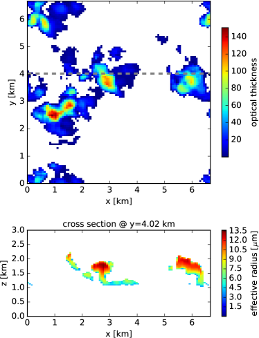
Figure 1: Definition of cumulus cloud field. The upper figure shows the integrated vertical optical thickness and the lower figure shows the effective radius for a vertical cross section (gray dashed line in upper figure) through the domain at $y$ = 4.02 km.

The upper panel in Figure 1 shows the vertically integrated optical thickness of the clouds and the lower panel shows the effective radius for a vertical cross section at y = 4.02 km.

The cloud optical properties have been computed using Mie theory [41, 42]. We assumed a gamma size distribution with an effective variance of 0.1, a value typical for liquid water clouds. The phase matrix ${\bf P}_{\rm C}$ for spherical particles has only 4 independent elements and it has the following form:

$${\bf P}_{\rm C}(\Theta)=\left[\begin{array}[]{cccc}P_{11}(\Theta)&P_{12}(\Theta)&0&0\\ P_{12}(\Theta)&P_{11}(\Theta)&0&0\\ 0&0&P_{33}(\Theta)&P_{34}(\Theta)\\ 0&0&-P_{34}(\Theta)&P_{33}(\Theta)\end{array}\right]$$ (18)

Figure 2 shows the scattering phase matrix at 400 nm for effective radii of 5 $\mu$m, 10 $\mu$m, and 15 $\mu$m, this is roughly the range we find in the cumulus cloud field.

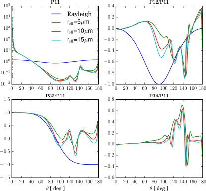
Figure 2: Phase matrix for Rayleigh scattering and liquid water cloud scattering.

We assumed that the surface is purely absorbing, i.e. the surface albedo was set to zero.

4 Results

4.1 Results for one-dimensional clear atmosphere

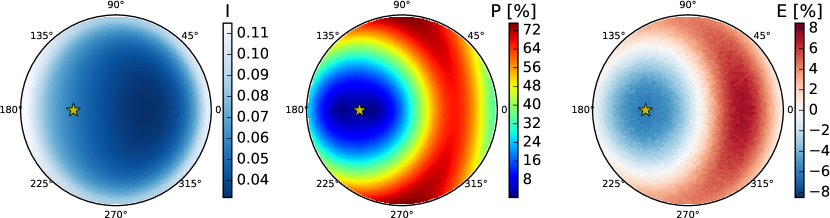
Figure 3: Normalized radiance, degree of polarization and error of scalar approximation at a wavelenth of 400 nm for the US-standard atmosphere for a down-looking observer at 120 km altitude. The sun position is ($\theta_{0},\phi_{0}$)=(40^∘, 0^∘) and the yellow star shows the viewing direction where the sun is in the back of the sensor ($\theta,\phi$)=(140^∘, 180^∘). The maximum overestimation is obtained for phase angles around 90^∘, and the maximum underestimation for backscattering directions close to a phase angle of 0^∘.

In order to provide an overview of the error due to neglecting polarization depending on viewing direction we calculate the radiance field at 120 km altitude (top of US-standard atmosphere) for a solar zenith angle $\theta_{0}$ of 40^∘ and a solar azimuth angle $\phi_{0}$ of 0^∘. The radiance in this and all other simulations has been normalized to the extraterrestrial irradiance. The left plot in Figure 3 shows the radiance for all viewing directions as a polar plot for the US-standard atmosphere at a wavelength of 400 nm. We see the typical Rayleigh scattering pattern with increasing radiances towards the horizon and smallest radiance values for directions, where the angle between incident solar radiation and viewing direction, the so-called phase angle, is about 90^∘. The middle plot shows the corresponding degree of polarization, which is smallest around the backscattering direction and largest at a phase angle of 90^∘. The right plot shows the error due to the scalar approximation. We find an overestimation of up to about 8% at a phase angle of about 90^∘ and an underestimation of up to about 7% in the backscattering region. These results are consistent with Mishchenko et al. [1], who explains the under- and overestimation by second-order and further low-order scattering processes. We also calculated the error for a sensor at the surface. The pattern of the results (not shown) is very similar to that for the sensor at the top of the atmosphere. For phase angles about 90^∘ the maximum overestimation of about 8% is obtained. In forward scattering directions, when the observer “looks” in a direction close to the sun, the radiance is underestimated by about 7%.

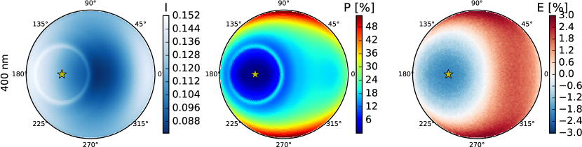
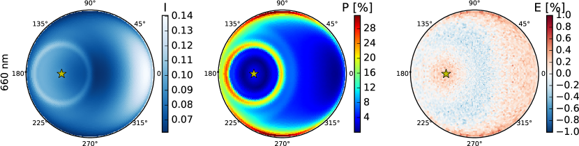
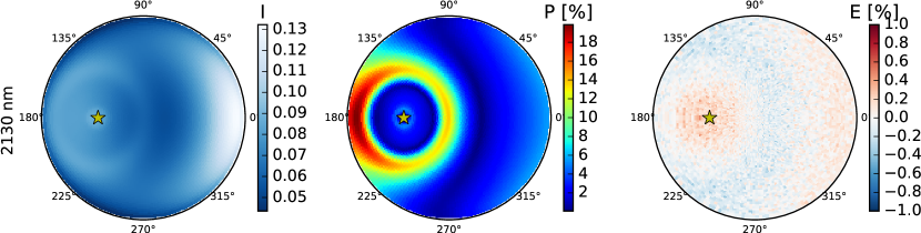
Figure 4: Normalized radiance, degree of polarization and error of scalar approximation for a down-looking observer at 120 km altitude. The sun position is ($\theta_{0},\phi_{0}$)=(40^∘, 0^∘) and the yellow star shows the viewing direction where the sun is in the back of the sensor ($\theta,\phi$)=(140^∘, 180^∘). A cloud layer with an optical thickness of 6 and droplets with an effective radius of 10 $\mu$m has been included at an altitude from 2–3 km into the US-standard molecular atmosphere. The rows correspond to wavelengths of 400 nm, 660 nm and 2130 nm.

Figure 4 shows the radiance, the degree of polarization and the error due to the neglect of polarization for a one-dimensional cloud layer. The rows correspond to wavelengths of 400 nm, 660 nm, and 2130 nm. The cloud consists of liquid water droplets with an effective radius of 10$\mu$m, is included in the layer from 2–3 km into the US-standard atmosphere, and it has an optical thickness of 6. The intensity and the degree of polarization show the strongly polarized cloudbow. At 400 nm the pattern is very similar as in Figure 3, thus the error is clearly dominated by Rayleigh scattering. The magnitude of the error is reduced from the range of $\pm$8% to about $\pm$3% due to multiple scattering.

At larger wavelengths (660 nm and 2130 nm) the angular pattern of the error changes: We find an overestimation due to the neglect of polarization around the backscattering direction and an underestimation in the cloudbow region. At scattering angles larger than about 90^∘ the scalar approximation slightly overestimates the radiance. Overall, for wavelengths of 660 nm and 2130 nm, the error is well below 1% for all viewing directions. For 95% of viewing directions the error is $<$0.3% at 660 nm, and $<$0.2% at 2130 nm. This result is not consistent with the calculations by Yi et al. [26] who investigated the impact of the neglect of polarization in radiative transfer calculations on cloud microphysical properties from MODIS observations: A closer look at Figure 4 (upper panel) in Yi et al. [26] reveals that for a cloud layer with an optical thickness of 6 and an effective droplet radius of 10 $\mu$m the differences between their vector and scalar radiance calculations at 650 nm is about 2%, certainly larger than the differences in our 1D cloud simulations. In order to explain these differences a radiative transfer model intercomparison would be required.

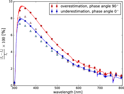
Figure 5: Maximum errors (overestimation in red and underestimation in blue) by the scalar approximation for US-standard atmosphere and a solar zenith angle of 40^∘ as a function of wavelength. The circles are simulations for a pure molecular atmosphere and the triangles are simulations with additional aerosols (continental average from OPAC). The small error bars correspond to 2 standard deviations of the Monte Carlo results.

Figure 5 shows the spectral dependence of the maximum overestimation and the maximum underestimation due to the scalar approximation. As in the previous simulation, we set the solar zenith angle to 40^∘ and the solar azimuth angle to 180^∘. The observer is located at the top of the atmosphere and we simulate two viewing directions given by the viewing zenith angle $\theta$ and the viewing azimuth angle $\phi$: (1) $(\theta,\phi)$=(50^∘, 0^∘) – for this direction the phase angle is 90^∘. (2) $(\theta,\phi)$=(40^∘, 180^∘) – this direction corresponds to backscattering (phase angle 0^∘), i.e. the sun is behind the observer. We choose these directions to estimate the maximum errors to be expected for Rayleigh scattering. The circles represent monochromatic simulations and the errorbars correspond to two standard deviations of the Monte Carlo results. In order to obtain the continuous spectrum including absorption features (solid lines) we have applied the absorption lines importance sampling method [43]. We find the maximum overestimation error of 9.5% at 335.5 nm and the maximum underestimation error of 8% at 329.5 nm. For smaller wavelenths the errors decrease due to strong ozone absorption and due to an increasing amount of multiple scattering and for larger wavelengths they decrease with decreasing Rayleigh scattering coefficient. The errors are also decreased in the absorption bands (e.g., oxygen-A absorption about 760 nm). Those results are consistent with Mishchenko et al. [1], who obtained decreasing errors for decreasing Rayleigh scattering optical thicknesses and decreasing single scattering albedos. The triangles in the figure show simulations including the US-standard atmosphere and in addition standard continental aerosol particles. We used the “continental average” aerosol as defined in the OPAC database and included in the libRadtran radiative transfer package [44, 30]. We find that the errors are only slightly reduced in presence of aerosols but are still significant (in the range between 8% at 350 nm and 1.5% at 800 nm).

Kotchenova et al. [13] have shown that for longer wavelengths and higher aerosol load, the error for aerosol scattering can be larger than for pure Rayleigh scattering. They find errors up to 5.3% at 670 nm wavelengths for an optically thick ($\tau$=0.728) biomass burning smoke aerosol model. The focus of this study is the error for realistic 3D atmospheres including clouds, therefore aerosols are not studied in more detail here.

4.2 Results for three-dimensional cloud field

Three-dimensional simulations are performed for the same sun-observer geometry as for the spectral calculation shown in the previous section and in addition for a phase angle of 40^∘ where cloud scattering produces high polarization (cloudbow, compare also Figure 2). In the following we show simulations performed at a wavelength of 400 nm.

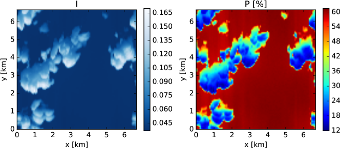
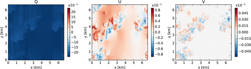
Figure 6: Top: Normalized Radiance and degree of polarization for a down-looking observer at 120 km altitude. The sun position is $(\theta_{0},\phi_{0})=(40^{\circ},90^{\circ})$ and the viewing direction is $(\theta,\phi)=(50^{\circ},270^{\circ})$, this corresponds to a phase angle of 90^∘. Bottom: Stokes vector components $Q$, $U$, and $V$.

Figure 6 shows the result for a phase angle of 90^∘  whereabouts we expect the maximum overestimation. The sun position is $(\theta_{0},\phi_{0})=(40^{\circ},90^{\circ})$ and the viewing direction is $(\theta,\phi)=(50^{\circ},270^{\circ})$. The upper left image shows the radiance $I$, which is increased on the illuminated sides of the clouds. Note that the direction of incident solar radiation is along the positive $y$-direction. The upper right image shows the degree of polarization, which is in the clear-sky region about 60%. Within the clouds it decreases to about 15% in illuminated regions and to about 35% in shadowed regions. The bottom images show the Stokes components $Q$, $U$, and $V$. Since the observation direction is in the solar principal plane, we find the major amount of polarization in the $Q$-component, which is negative, thus the radiation is polarized perpendicular to the scattering plane which we expect for Rayleigh scattering at 90^∘ scattering angle. The cloud scattering contribution to $Q$ is small in this sun-observer geometry, thus the clouds are barely visible in the $Q$-image. The components $U$ and $V$ would be exactly 0 for plane-parallel simulations for symmetry reasons. Since the 3D clouds are not symmetric about the scattering plane we obtain polarization patterns for $U$ and $V$. For $U$ we see that the polarization propagates from the clouds into the clear region by multiple scattering. $U$ has positive and negative values being 1–2 orders of magnitude smaller than $Q$. We find small circular polarization in the clouds, however $V$ is almost 3 orders of magnitue smaller than $Q$. It should be noted, that the strong decrease of the degree of polarization in the cloud can mainly be attributed to the increase of the radiance $I$.

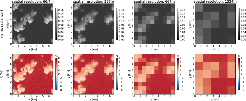
Figure 7: Normalized radiance (top) and error due to neglect of polarization (bottom) for various spatial resolutions. The simulations are for a phase angle of 90^∘, where the scalar approximation yields an overestimation of the radiance $I$.

Figure 7 shows the radiance field (top panels) and the error (overestimation) due to the neglect of polarization (bottom panels). The left figure is simulated with the same spatial resolution as the input cloud field (66.7 m $\times$ 66.7 m). The result shows, that in the clear-sky region between the clouds, the overestimation is about 6%. The simulation without clouds (compare previous section) yields an overestimation of about 8%, thus cloud scattering into the clearsky regions reduces the error by about 2%. In the cloud shadow regions the overestimation is of the order of 4%. To assess the question, whether it is important to consider polarization in radiative transfer simulations for satellite remote sensing instruments, we average the result to mimic coarser resolutions: we calculate block mean averages of 4$\times$4, 10$\times$10 and 20$\times$20 pixels, respectively. This way we obtain similar spatial resolutions as for example the MODIS instrument with spatial resolutions of 250 m (e.g. for band 1, bandwidth 620–670 nm), 500 m (e.g. band 3, bandwith 459–479 nm) and 1000 m (e.g. band 8, bandwidth 405–420 nm). In the averaged radiance images the fine cumulus cloud structures are no longer well resolved. The error patterns are similar to the image with highest resolution, with errors ranging from about 4% in cloud shadow regions to about 6% in the clear sky region. Many of the pixels are partially cloudy with errors ranging from about 2–5.5%. Thus the neglect of polarization can cause significant errors at short wavelengths, in particular when the observed pixels are mostly partially cloudy or include cloud shadows.

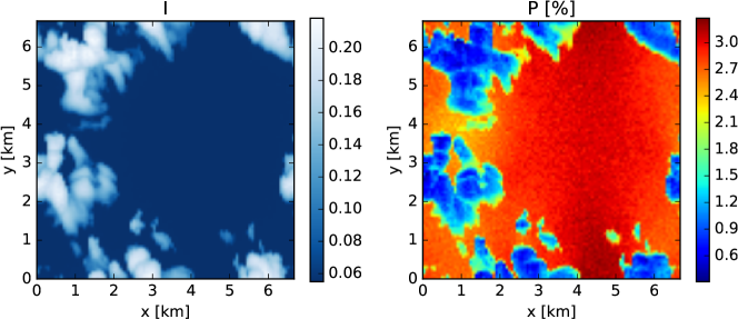
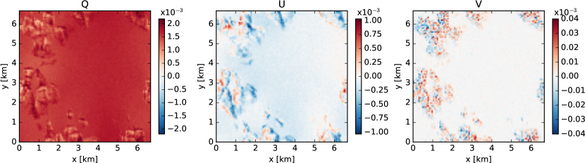
Figure 8: Top: Normalized radiance and degree of polarization for an observer at the top of the atmosphere ($(\theta_{0},\phi_{0})=(40^{\circ},90^{\circ}),(\theta,\phi)=(40^{\circ},90^{\circ})$). The phase angle is 0^∘(backscattering direction). Bottom: Stokes vector components $Q$, $U$, and $V$.

The upper plots in Figure 8 show the radiance field and the degree of polarization in backscattering direction. In the radiance image the clouds appear bright and in this geometry the clouds do not shadow other parts of the clouds as much as for a phase angle of 90^∘ (compare Figure 6). The degree of polarization in backscattering direction is very small, about 3% in the clear regions and below 1% in cloudy regions. In regions with optically thin clouds the degree of polarization is between 1% and 3% and for optically thicker clouds it becomes close to 0. In backscattering direction $Q$ is positive, thus the radiation is polarized parallel to the scattering plane as expected for Rayleigh scattering. The clouds partly increase and partly decrease $Q$. The Stokes component $U$, which is exactly 0 for backscattering in a one-dimensional model, shows a pattern generated by scattering in the three-dimensional clouds. Further, small circular polarization (non-zero $V$) can be observed in the clouds.

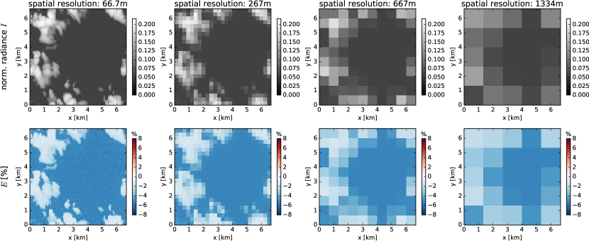
Figure 9: Normalized radiance (top) and error due to neglect of polarization (bottom) for various spatial resolutions. The simulations are for a phase angle of 0^∘, where the scalar approximation yields an underestimation of the radiance $I$.

Figure 9 shows the underestimation due to the scalar approximation for various spatial resolutions in backscattering direction. In the clear sky regions it is about 5%, this is about 1.5% less compared to a pure Rayleigh atmosphere. In the cloudy regions the error is mostly below 2%. For partially cloudy pixels the error of the scalar approximation is significant, depending on the cloud cover we find values between 3 and 5%.

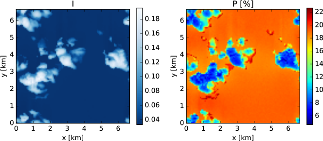
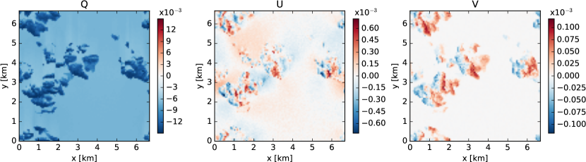
Figure 10: Top: Normalized radiance and degree of polarization for an observer at the top of the atmosphere ($(\theta_{0},\phi_{0})=(40^{\circ},90^{\circ}),(\theta,\phi)=(0^{\circ},0^{\circ})$). The phase angle is 40^∘(cloudbow direction). Bottom: Stokes components $Q$, $U$, and $V$.

The upper images in Figure 10 show the radiance field and the degree of polarization for a phase angle of 40^∘, corresponding to the cloudbow, where cloud scattering is highly polarized. This can be seen in the image of $Q$ (lower left plot), the absolute value of which is much larger in the clouds than in the clearsky background. Nevertheless the degree of polarization is mostly smaller in the clouds than in the clear regions, because the increase of $I$ by multiple scattering is larger than the increase of $Q$ which depends on fewer orders of scattering. Only for very thin clouds the degree of polarization is increased compared to clear sky. The viewing direction is nadir, still we find non-zero $U$ and $V$ patterns due to the asymmetric cloud structures.

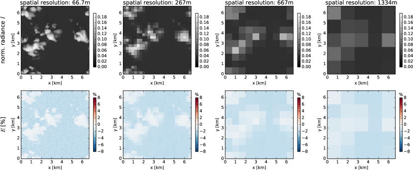
Figure 11: Normalized radiance (top) and error due to neglect of polarization (bottom) for various spatial resolutions. The simulations are for a phase angle of 40^∘, where the scalar approximation yields an underestimation of the radiance $I$.

Fig. 11 shows the radiance and the error due to the neglect of polarization for various spatial resolutions. We find that the radiance is underestimated, in the clear region by approximately 2%. Corresponding 1D simulations yield an underestimation of about 2.7%. In the cloudy and partially cloudy parts of the image the error is always below 2%. These results show, that the error due to the neglect of polarization is caused by Rayleigh scattering, even in a sun-observer geometrie where cloud scattering causes significant polarization.

We have performed the simulations in cloudbow geometry for wavelengths relevant for cloud remote sensing, namely 660 nm and 2130 nm (not shown). For 660 nm we obtain a maximum underestimation of 0.7% in the clear part of the image and even smaller errors in the cloudy regions. For 2130 nm the error is below 0.5% in the whole image.

5 Summary and conclusions

We have investigated the error due to the neglect of polarization in radiative transfer calculations for a realistic three-dimensional atmosphere.

First, in order to get an idea of the error distribution depending on viewing direction and sensor position, we have calculated the error for all viewing directions from the surface as well as from space. We have used the US-standard (multi-layer) atmosphere, and performed radiative transfer simulations at a wavelength of 400 nm in full vector and in scalar mode, respectively, and calculate the relative difference between the obtained radiances. In accordance to Mishchenko et al. [1] we find the maximum overestimation of about 8% for a phase angle of 90^∘ and the maximum underestimation of about 6.5% for phase angles of 0^∘ or 180^∘. For other viewing directions, the error is between these two extreme values.

The same simulations including a homogeneous cloud layer yield errors smaller than 3% at 400 nm for all sun-observer geometries, including the cloudbow region where cloud scattering causes high polarization. For larger wavelengths (660 nm and 2130 nm) the errors are generally well below 1%.

Next, we investigated the spectral dependance of the maximum over-/underestimation. As expected we find that it decreases from about 9.5%/7.5% at 350 nm to about 1.3%/1% at 800 nm as the Rayleigh optical thickness decreases. In the water vapor and oxygen absorption bands the error is also decreased, this result is again consistent with Mishchenko et al. [1] who showed that the error decreases with decreasing single scattering albedo. We found that for typical continental average aerosol conditions the error is decreased by 1–2% at shorter wavelengths up to about 500 nm. At longer wavelengths the magnitude of the error is not changed by this type of aerosol.

Finally, we performed simulations for a three-dimensional cloud field surrounded by the US-standard molecular atmosphere. The spatial resolution of the cloud field is 66.7 m $\times$ 66.7 m and the domain size is 6.67 km $\times$ 6.67 km. We simulated 100$\times$100 pixels for a sensor located at the top of the atmosphere.

In order to obtain the maximum errors that can be expected due to Rayleigh scattering, we simulated two viewing directions corresponding to phase angles of 90^∘ and 0^∘, respectively. In the clear regions between the clouds we find that the overestimation error is about 6%, which is approximately 2% less than in the pure clear-sky atmosphere without surrounding clouds. The reason for this decrease is that photons which are multiple scattered in the clouds enter the clear-sky region without a preferred direction. When those photons are scattered by molecules towards the observer, they do not have a preferred polarization direction. Within the clouds the error is still up to 4% with largest values in shadowed regions. In order to simulate coarser spatial resolutions including partially cloudy pixels we spatially averaged our results over 267 m, 667 m, and 1334 m, respectively. Those results are typical for satellite observations with coarser resolutions. We find that in the partially cloudy pixels the overestimation error ranges from 2-5.5%. The underestimation errors are generally slightly smaller than the overestimation errors.

In order to test whether scattering at cloud droplets cause significant errors we performed 3D simulations at a phase angle of 40^∘ corresponding to the highly polarized cloudbow. At 400 nm, where the Rayleigh scattering contribution is large, we find errors of up to 2% in the region between the clouds and smaller errors within the clouds. At 660 nm and 2130 nm, wavelengths that are typically used for cloud remote sensing, the errors are less than 1% in the full domain.

In summary, our results show that the error due to the neglect of polarization is not always negligible for radiative transfer in realistic clouds at shorter wavelengths with significant Rayleigh scattering contribution. As shown in Figure 5 the error decreases with wavelengths as the amount of Rayleigh scattering decreases.

Many cloud retrieval algorithms utilize longer wavelengths, as for instance the widely used lookup-table method by Nakajima and King [17], which has been developed for observations at 750 nm and at 2160 nm. For the operational cloud properties retrieval algorithms from MODIS observations this method has been adapted for various channel combinations using spectral bands in the range from 0.67 $\mu$m to 3.7 $\mu$m [45]. Our results suggest that for this type of cloud retrieval algorithms the scalar approximation can safely be applied. However, Yi et al. [26] found that the neglect of polarization in the radiative transfer simulations produce errors as large as 15% in retrieved cloud optical thickness and effective droplet radius. They do not analyse in detail the cases which produce the very large errors. In our one-dimensional radiative transfer simulations we did not find sun-observer geometries which would produce such large errors.

For hyperspectral retrieval methods the error might be relevant. E.g., the algorithm by Zinner et al. [19] utilizes the spectral slope of the radiance between 485 and 560 nm. In this range the maximum error due to the scalar approximation for Rayleigh scattering changes from about 6% to 4%, so that the spectral slope will be affected by the scalar approximation.

The scalar approximation could also have a significant impact on aerosol and cloud retrieval algorithms for multi-angle multi-spectral observations (e.g., the Multi-angle Imaging SpectroRadiometer MISR), because the error strongly depends on observation direction; for some directions the error is negligible while for others it might be several per cent, in particular for wavelengths below 500 nm that are used for aerosol remote sensing.

References

- Mishchenko et al. [1994] M. I. Mishchenko, A. A. Lacis, L. D. Travis, Errors induced by the neglect of polarization in radiance calculations for Rayleigh-scattering atmospheres, J. Quant. Spectrosc. Radiat. Transfer 51 (3) (1994) 491–510, ISSN 0022-4073, doi:–10.1016/0022-4073(94)90149-X˝.
- Hansen [1971] J. E. Hansen, Multiple scattering of polarized light in planetary atmospheres. Part II: Sunlight reflected by terrestrial water clouds, J. Atmos. Sci. 28 (8) (1971) 1400–1426.
- Chandrasekhar [1950] S. Chandrasekhar, Radiative Transfer, Oxford Univ. Press, UK, 1950.
- Hansen and Travis [1974] J. E. Hansen, L. D. Travis, Light scattering in planetary atmospheres, Space Science Reviews 16 (1974) 527–610.
- de Haan et al. [1987] J. F. de Haan, P. B. Bosma, J. W. Hovenier, The adding method for multiple scattering calculations of polarized light, Astronomy and Astrophysics 183 (1987) 371–391.
- Doicu et al. [2013] A. Doicu, D. Efremenko, T. Trautmann, A multi-dimensional vector spherical harmonics discrete ordinate method for atmospheric radiative transfer, J. Quant. Spectrosc. Radiat. Transfer 118 (2013) 121–131.
- Collins et al. [1972] D. G. Collins, W. G. Blättner, M. B. Wells, H. G. Horak, Backward Monte Carlo calculations of the polarization characteristics of the radiation emerging from spherical-shell atmospheres., Appl. Opt. 11 (1972) 2684–2696.
- Emde et al. [2010] C. Emde, R. Buras, B. Mayer, M. Blumthaler, The impact of aerosols on polarized sky radiance: model development, validation, and applications, Atmos. Chem. Phys. 10 (2) (2010) 383–396.
- Cornet et al. [2010] C. Cornet, L. C-Labonnote, F. Szczap, Three-dimensional polarized Monte Carlo atmospheric radiative transfer model (3DMCPOL): 3D effects on polarized visible reflectances of a cirrus cloud, J. Quant. Spectrosc. Radiat. Transfer 111 (1) (2010) 174 – 186, ISSN 0022-4073, doi:http://dx.doi.org/10.1016/j.jqsrt.2009.06.013.
- Stamnes et al. [2000] K. Stamnes, S.-C. Tsay, W. Wiscombe, I. Laszlo, DISORT, a General-Purpose Fortran Program for Discrete-Ordinate-Method Radiative Transfer in Scattering and Emitting Layered Media: Documentation of Methodology, Tech. Rep., Dept. of Physics and Engineering Physics, Stevens Institute of Technology, Hoboken, NJ 07030, 2000.
- Buras et al. [2011] R. Buras, T. Dowling, C. Emde, New secondary-scattering correction in DISORT with increased efficiency for forward scattering, J. Quant. Spectrosc. Radiat. Transfer 112 (12) (2011) 2028–2034.
- Adams and Kattawar [1970] C. N. Adams, G. W. Kattawar, Solutions of equations of radiative transfer by an invariant imbedding approach, J. Quant. Spectrosc. Radiat. Transfer 10 (5) (1970) 341–&, ISSN 0022-4073, doi:–10.1016/0022-4073(70)90101-9˝.
- Kotchenova et al. [2006] S. Y. Kotchenova, E. F. Vermote, R. Matarrese, J. Frank J. Klemm, Validation of a vector version of the 6S radiative transfer code for atmospheric correction of satellite data. Part I: Path radiance, Appl. Opt. 45 (2006) 6762–6774.
- Mishchenko [2014] M. I. Mishchenko, Directional radiometry and radiative transfer: The convoluted path from centuries-old phenomenology to physical optics, J. Quant. Spectrosc. Radiat. Transfer 146 (SI) (2014) 4–33, ISSN 0022-4073, doi:–10.1016/j.jqsrt.2014.02.033˝.
- Waquet et al. [2007] F. Waquet, P. Goloub, J.-L. Deuze, J.-F. Leon, F. Auriol, C. Verwaerde, J.-Y. Balois, P. Francois, Aerosol retrieval over land using a multiband polarimeter and comparison with path radiance method, J. Geophys. Res. 112 (D11), doi:10.1029/2006JD008029.
- Barlakas [2016] V. Barlakas, A New Three–Dimensional Vector Radiative Transfer Model and Applications to Saharan Dust Fields, Ph.D. thesis, University of Leipzig, Faculty of Physics and Earth Sciences, URL http://www.qucosa.de/recherche/frontdoor/?tx_slubopus4frontend[id]=20746, 2016.
- Nakajima and King [1990] T. Nakajima, M. D. King, Determination of the optical thickness and effective particle radius of clouds from reflected solar radiation measurements. Part I: theory, Journal of the Atmospheric Sciences 47 (15) (1990) 1878–1893.
- Zinner et al. [2010] T. Zinner, G. Wind, S. Platnick, A. S. Ackerman, Testing remote sensing on artificial observations: impact of drizzle and 3-D cloud structure on effective radius retrievals, Atmos. Chem. Phys. 10 (19) (2010) 9535–9549.
- Zinner et al. [2016] T. Zinner, P. Hausmann, F. Ewald, L. Bugliaro, C. Emde, B. Mayer, Ground-based imaging remote sensing of ice clouds: uncertainties caused by sensor, method and atmosphere, Atmospheric Measurement Techniques 9 (9) (2016) 4615–4632, doi:10.5194/amt-9-4615-2016, URL https://www.atmos-meas-tech.net/9/4615/2016/.
- Levis et al. [2015] A. Levis, Y. Y. Schechner, A. Aides, A. B. Davis, Airborne Three-Dimensional Cloud Tomography, in: The IEEE International Conference on Computer Vision (ICCV), 2015.
- Levis et al. [2017] A. Levis, Y. Y. Schechner, A. B. Davis, Multiple-Scattering Microphysics Tomography, in: the 30th IEEE/CVF Conference on Computer Vision and Pattern Recognition (CVPR17), 2017.
- Evans [1998] K. F. Evans, The spherical harmonics discrete ordinate method for three–dimensional atmospheric radiative transfer, J. Atmos. Sci. 55 (1998) 429–446.
- Deschamps et al. [1994] P.-Y. Deschamps, F.-M. Breon, M. Leroy, A. Podaire, A. Bricaud, J.-C. Buriez, G. Seze, The POLDER mission: instrument characteristics and scientific objectives, IEEE Transactions on Geoscience and Remote Sensing 32 (1994) 598–615, doi:10.1109/36.297978.
- Bréon and Doutriaux-Boucher [2005] F.-M. Bréon, M. Doutriaux-Boucher, A comparison of Cloud Droplet Radii Measured from Space, IEEE Transactions on Geoscience and Remote Sensing 43 (8) (2005) 1769–1805.
- Stap et al. [2016] F. A. Stap, O. P. Hasekamp, C. Emde, T. Rockmann, Multiangle photopolarimetric aerosol retrievals in the vicinity of clouds: Synthetic study based on a large eddy simulation, J. Geophys. Res. 121 (21) (2016) 12914–12935, ISSN 2169-897X, doi:–10.1002/2016JD024787˝.
- Yi et al. [2014] B. Yi, X. Huang, P. Yang, B. A. Baum, G. W. Kattawar, Considering polarization in MODIS-based cloud property retrievals by using a vector radiative transfer code, J. Quant. Spectrosc. Radiat. Transfer 146 (SI) (2014) 540–548, doi:10.1016/j.jqsrt.2014.05.020.
- Mayer [2009] B. Mayer, Radiative transfer in the cloudy atmosphere, European Physical Journal Conferences 1 (2009) 75–99.
- Mishchenko et al. [2006] M. I. Mishchenko, L. D. Travis, A. A. Lacis, Multiple Scattering of Light by Particles: Radiative Transfer and Coherent Backscattering, Cambridge University Press, 2006.
- Mishchenko [2006] M. I. Mishchenko, Radiative transfer in clouds with small-scale inhomogeneities: Microphysical approach, J. Geophys. Res. 33 (14), doi:10.1029/2006GL026312.
- Emde et al. [2016] C. Emde, R. Buras-Schnell, A. Kylling, B. Mayer, J. Gasteiger, U. Hamann, J. Kylling, B. Richter, C. Pause, T. Dowling, L. Bugliaro, The libRadtran software package for radiative transfer calculations (version 2.0.1), Geophy. Mod. Dev. 9 (5) (2016) 1647–1672, doi:10.5194/gmd-9-1647-2016, URL http://www.geosci-model-dev.net/9/1647/2016/.
- Mayer and Kylling [2005] B. Mayer, A. Kylling, Technical note: The libRadtran software package for radiative transfer calclations – description and examples of use, Atmos. Chem. Phys. 5 (2005) 1855–1877.
- Buras and Mayer [2011] R. Buras, B. Mayer, Efficient unbiased variance reduction techniques for Monte Carlo simulations of radiative transfer in cloudy atmospheres: The solution, J. Quant. Spectrosc. Radiat. Transfer 112 (3) (2011) 434–447.
- Cahalan et al. [2005] R. Cahalan, L. Oreopoulos, A. Marshak, K. Evans, A. Davis, R. Pincus, K. Yetzer, B. Mayer, R. Davies, T. Ackerman, B. H.W., E. Clothiaux, R. Ellingson, M. Garay, E. Kassianov, S. Kinne, A. Macke, W. O’Hirok, P. Partain, S. Prigarin, A. Rublev, G. Stephens, F. Szczap, E. Takara, T. Varnai, G. Wen, T. Zhuraleva, The International Intercomparison of 3D Radiation Codes (I3RC): Bringing together the most advanced radiative transfer tools for cloudy atmospheres, Bulletin of the American Meteorological Society 86 (9) (2005) 1275–1293.
- Kokhanovsky et al. [2010] A. A. Kokhanovsky, V. P. Budak, C. Cornet, M. Duan, C. Emde, I. L. Katsev, D. A. Klyukov, S. V. Korkin, L. C-Labonnote, B. Mayer, Q. Min, T. Nakajima, Y. Ota, A. S. Prikhach, V. V. Rozanov, T. Yokota, E. P. Zege, Benchmark results in vector atmospheric radiative transfer, J. Quant. Spectrosc. Radiat. Transfer 111 (12-13) (2010) 1931–1946.
- Emde et al. [2015] C. Emde, V. Barlakas, C. Cornet, F. Evans, S. Korkin, Y. Ota, L. C. Labonnote, A. Lyapustin, A. Macke, B. Mayer, M. Wendisch, IPRT polarized radiative transfer model intercomparison project - Phase A, J. Quant. Spectrosc. Radiat. Transfer 164 (0) (2015) 8–36, ISSN 0022-4073, doi:10.1016/j.jqsrt.2015.05.007, URL http://www.sciencedirect.com/science/article/pii/S0022407315001922.
- Emde et al. [2018] C. Emde, V. Barlakas, C. Cornet, F. Evans, Z. Wang, L. C. Labonotte, A. Macke, B. Mayer, M. Wendisch, IPRT polarized radiative transfer model intercomparison project – Three-dimensional test cases (phase B), J. Quant. Spectrosc. Radiat. Transfer 209 (2018) 19–44, ISSN 0022-4073, doi:10.1016/j.jqsrt.2018.01.024, URL https://www.sciencedirect.com/science/article/pii/S0022407317308981.
- Anderson et al. [1986] G. Anderson, S. Clough, F. Kneizys, J. Chetwynd, E. Shettle, AFGL atmospheric constituent profiles (0-120 km), Tech. Rep. AFGL-TR-86-0110, Air Force Geophys. Lab., Hanscom Air Force Base, Bedford, Mass., 1986.
- Bodhaine et al. [1999] B. A. Bodhaine, N. B. Wood, E. G. Dutton, J. R. Slusser, On Rayleigh optical depth calculations, J. Atm. Ocean Technol. 16 (1999) 1854–1861.
- Gasteiger et al. [2014] J. Gasteiger, C. Emde, B. Mayer, R. Buras, S. Buehler, O. Lemke, Representative wavelengths absorption parameterization applied to satellite channels and spectral bands, J. Quant. Spectrosc. Radiat. Transfer 148 (0) (2014) 99 – 115.
- Stevens et al. [1999] B. Stevens, C. H. Moeng, P. P. Sullivan, Large-eddy simulations-of radiatively driven convection: Sensitivities to the representation of small scales, J. Atmos. Sci. 56 (1999) 3963–3984.
- Mie [1908] G. Mie, Beiträge zur Optik trüber Medien, speziell kolloidaler Metallösungen, Annalen der Physik 330 (1908) 377–445, doi:10.1002/andp.19083300302.
- Wiscombe [1980] W. Wiscombe, Improved Mie scattering algorithms, Appl. Opt. 19 (9) (1980) 1505–1509.
- Emde et al. [2011] C. Emde, R. Buras, B. Mayer, ALIS: An efficient method to compute high spectral resolution polarized solar radiances using the Monte Carlo approach, J. Quant. Spectrosc. Radiat. Transfer 112 (10) (2011) 1622–1631.
- Hess et al. [1998] M. Hess, P. Koepke, I. Schult, Optical Properties of Aerosols and Clouds: The Software Package OPAC, Bulletin of the American Meteorological Society 79 (5) (1998) 831–844.
- Platnick et al. [2017] S. Platnick, K. G. Meyer, M. D. King, G. Wind, N. Amarasinghe, B. Marchant, G. T. Arnold, Z. Zhang, P. A. Hubanks, R. E. Holz, P. Yang, W. L. Ridgway, J. Riedi, The MODIS Cloud Optical and Microphysical Products: Collection 6 Updates and Examples From Terra and Aqua, IEEE Transactions on Geoscience and Remote Sensing 55 (1) (2017) 502–525, ISSN 0196-2892, doi:10.1109/TGRS.2016.2610522.