IPRT polarized radiative transfer model intercomparison project – three-dimensional test cases (phase B)

Abstract

Initially unpolarized solar radiation becomes polarized by scattering in the Earth’s atmosphere. In particular molecular scattering (Rayleigh scattering) polarizes electromagnetic radiation, but also scattering of radiation at aerosols, cloud droplets (Mie scattering) and ice crystals polarizes. Each atmospheric constituent produces a characteristic polarization signal, thus spectro-polarimetric measurements are frequently employed for remote sensing of aerosol and cloud properties.

Retrieval algorithms require efficient radiative transfer models. Usually, these apply the plane-parallel approximation (PPA), assuming that the atmosphere consists of horizontally homogeneous layers. This allows to solve the vector radiative transfer equation (VRTE) efficiently. For remote sensing applications, the radiance is considered constant over the instantaneous field-of-view of the instrument and each sensor element is treated independently in plane-parallel approximation, neglecting horizontal radiation transport between adjacent pixels (Independent Pixel Approximation, IPA). In order to estimate the errors due to the IPA approximation, three-dimensional (3D) vector radiative transfer models are required.

So far, only a few such models exist. Therefore, the International Polarized Radiative Transfer (IPRT) working group of the International Radiation Commission (IRC) has initiated a model intercomparison project in order to provide benchmark results for polarized radiative transfer. The group has already performed an intercomparison for one-dimensional (1D) multi-layer test cases [phase A, Emde et al., 2015]. This paper presents the continuation of the intercomparison project (phase B) for 2D and 3D test cases: a step cloud, a cubic cloud, and a more realistic scenario including a 3D cloud field generated by a Large Eddy Simulation (LES) model and typical background aerosols.

The commonly established benchmark results for 3D polarized radiative transfer are available at the IPRT website (http://www.meteo.physik.uni-muenchen.de/~iprt).

1 Introduction

The polarization state of electromagnetic radiation includes characteristic information about the particles, at which the radiation has been scattered. This is used by various remote sensing methodologies to retrieve information about aerosol and cloud optical and microphysical properties.

One of the most prominent instruments that measure polarization is the Polarization and Directionality of the Earth’s Reflectances (POLDER) instrument which was operated onboard the PARASOL (Polarization and Anisotropy of Reflectances for Atmospheric Sciences coupled with Observations from a Lidar) satellite [Deschamps et al., 1994] and has provided useful observations from 2004–2013. The PARASOL mission has demonstrated the usefulness of multi-spectral directional polarized measurements. With polarization, it is possible to retrieve the size distribution of cloud droplets at the top of cloud with high accuracy [Bréon and Doutriaux-Boucher, 2005]. Further, one can retrieve aerosol optical properties over bright surfaces such as clouds [Waquet et al., 2013] or land [Dubovik et al., 2011, Xu et al., 2017], which is not possible from unpolarized observations where a dark background is required. Moreover, surface properties, i.e. bidirectional polarized reflectance functions can be derived [Maignan et al., 2009].

The next satellite mission including an instrument similar to POLDER will be the Multi-Viewing Multi-Channel Multi-Polarization Imaging mission (3MI) on METOP-SG (Meteorological Operational Satellite - Second Generation) planned to be launched in 2021 [Marbach et al., 2015]. Further planned satellite missions with polarimeters on board include the Aerosol, Cloud, ocean Ecosystem (ACE) mission, the MAIA (Multi-Angle Imager for Aerosols) mission [Liu and Diner, 2017], and the PACE (Plankton, Aerosol, Cloud, ocean Ecosystem) mission (https://pace.gsfc.nasa.gov/).

There are several airborne prototype polarimeters for the preparation of these missions. The ACE Polarimeter Working Group (ACEPWG, https://earthscience.arc.nasa.gov/ACEPWG) is a forum for sharing calibration techniques and geophysical parameter retrieval methods. It also performs intercomparison of the data collected in field campaigns. Participating instruments are the airborne prototypes of the Multi-angle SpectroPolarimetric Imager (AirMSPI) [Diner et al., 2012], the Hyper-Angular Rainbow Polarimeter (AirHARP), the Spectropolarimeter for Planetary Exploration (AirSPEX) [van Harten et al., 2011], and the Research Scanning Polarimeter (RSP) [Cairns et al., 1999, 2003].

AERONET (AErosol RObotic Network) is a federation of ground-based remote sensing aerosol networks. It includes the commercially available ground-based polarimeter, CE318-DP, developed by CIMEL Electronic (Paris, France) at many stations.

For correct aerosol retrievals from airborne, satellite or ground-based polarimetric observations, in particular in partially cloudy scenes, three-dimensional (3D) radiative transfer models are required. Davis et al. [2013] studied the influence of 3D effects on 1D aerosol retrievals from the APS (Aerosol Polarimetry Sensor) instrument, which was launched with the Glory mission [Mishchenko et al., 2007], but that failed, unfortunately. Similarly, 3D effects on aerosol retrievals from POLDER observations have been investigated by Stap et al. [2016a], Stap et al. [2016b] and Cornet et al. [2017]. For aerosol retrievals in partially cloudy scenes, retrieval errors become significant in the vicinity of clouds. This effect is also known for aerosol retrievals from unpolarized observations, e.g. from MODIS [Wen et al., 2013, Várnai et al., 2013]. An adjoint method for adjusting 3D atmosphere and surface properties to fit polarimetric measurements has been derived by Martin et al. [2014] and Martin and Hasekamp [2018]. However, to our knowledge, this method has not been applied to real data so far. A tomographic cloud reconstruction method, which uses the 3D SHDOM radiative transfer code [Evans, 1998] as forward model, has been developed for scalar multi-angle solar observations [Levis et al., 2015, 2017]. The method has successfully been applied to AirMSPI measurements to retrieve cloud extinction coefficient, effective droplet size and cloud liquid water content. The influence of 3D effects on polarimetric cloud droplet size retrievals was investigated by Alexandrov et al. [2012] and they found that 3D effects are negligible, thus the PPA can safely be used in the forward model of their retrieval algorithm. Cornet et al. [2017] studied the influence of 3D effects on cloud parameter retrievals from POLDER observations. Their results confirm that the droplet size retrieval is not much affected by 3D effects. Barlakas et al. [2016] and Barlakas [2016] investigated the errors induced by neglecting horizontal radiation transport and domain heterogeneities including polarization in LIDAR-measured dust fields. The differences in domain-averaged normalized radiances between PPA/IPA and 2D calculations are insignificant. However, in the areas with large spatial variability in optical thickness, the radiance fields of the 2D calculations differ about 20% for radiance and polarization from the fields of the PPA. Barlakas [2016] also investigated the error which is induced by neglecting polarization in scalar radiative transfer: For pure Rayleigh scattering errors up to 10.5% are found for the scalar radiance, in agreement to former studies (e.g. Kotchenova et al. [2006]). For 1D and 2D inhomogeneous atmospheres with Sahara dust aerosols, the maximum error is less than 1%, which is explained by relatively high optical thickness und thus high-order multiple scattering and the asymmetric scattering phase matrices of the dust particles.

All aforementioned studies used 3D vector radiative transfer models. So far, all these codes have not been validated regarding 3D geometry, since established benchmark data does not exist. Previous model intercomparisons cover e.g. 3D scalar radiative transfer (I3RC – Intercomparison of 3D radiation Codes, [Cahalan et al., 2005]), scalar radiative transfer in 1D spherical geometry [Loughman et al., 2004], scalar radiative transfer in the millimeter/submillimeter spectral region [Melsheimer et al., 2005], or 1D vector radiative transfer [Kokhanovsky et al., 2010, Emde et al., 2015]. The IPRT intercomparison project presented in this article aims to provide benchmark results for 3D vector radiative transfer. The project webpage http://www.meteo.physik.uni-muenchen.de/~iprt provides input data and results of all models, so that the test cases may be reproduced by 3D vector radiative transfer modelers for validation purposes.

Section 2 provides an overview of the participating radiative transfer models. In Section 3, general definitions as the coordinate system are provided. Section 4 presents the model intercomparison for the most simple setup, a step cloud. In Section 5, we present the results for a cubic cloud. Section 6 shows the most realistic simulations for an LES cloud field. Finally, a brief summary is given in Section 7.

2 Radiative transfer models

Table 1: Overview of radiative transfer models

model name	method	geometry	arbitrary output altitude	references
3DMCPOL	Monte Carlo	1D/3D	yes	Cornet et al. [2010], Fauchez et al. [2014]
MSCART	Monte Carlo	1D/3D	yes	Wang et al. [2017]
MYSTIC	Monte Carlo	1D/3D(a)	yes	Mayer [2009], Emde et al. [2010, 2016]
SHDOM	spherical harmonics discrete ordinate	1D/3D	yes	Evans [1998], Emde et al. [2015]
SPARTA	Monte Carlo	1D/3D	no	Barlakas et al. [2016], Barlakas [2016]
(a)MYSTIC includes fully spherical geometry for 1D and 3D.

Table 1 gives an overview of the participating radiative transfer models. In the following, only the MSCART model is briefly described. For short descriptions of the other models please refer to the first publication of the IPRT project [Emde et al., 2015].

2.1 MSCART

MSCART (Multiple-Scaling-based Cloudy Atmospheric Radiative Transfer) is a universal simulator of scalar and vector Monte Carlo radiative transfer in 3D cloudy atmospheres. It is the successor of the radiative transfer code of MCRT [Wang et al., 2011, 2012]. MSCART has established a unified forward and backward scattering order-dependent integral radiative transfer theoretical framework [Wang et al., 2017], which can generalize the model with variance reduction formalism in a wide range of simulation scenarios. These include 3D atmospheres with molecules, aerosols and clouds and 2D surfaces (Lambertian and BPDF (Bidirectional Polarized reflectance Distribution Function)).

The model is coded in an object-oriented programming architecture using modern Fortran language [Wang et al., 2017]. This gives the MSCART code a good maintainability and reusability, and an enhanced capability to add new features in future. Through several years of development, the model has become a versatile and sound tool for passive and active remote sensing applications. In forward mode, it can simulate average radiances over horizontal areas in specified directions for sunlight and range-resolved backscattering signals for laser source; in backward mode, it not only simulates average radiances over horizontal areas in specified directions but also gives radiances at specified locations in specified directions for the solar spectral range. Polarization has been recently added to the model for macroscopically isotropic and mirror-symmetric scattering medium.

More importantly, sophisticated variance reduction techniques are implemented into the model to speedup simulations for cloudy atmospheres with highly forward-peaked scattering. The previous studies reduce variance either by using the scattering phase matrix forward truncation technique or the target directional importance sampling technique. In this model, a novel scattering order-dependent variance reduction method is used to combine both of them and a new scattering order sampling algorithm is implemented to achieve an order-dependent tuning parameter optimization [Wang et al., 2017]. The MSCART software package with several simulation examples can be freely downloaded after registration from the designated website http://mscart.nuist.edu.cn.

3 General definitions

3.1 Model coordinate system and Stokes vector

For all test cases, the four Stokes parameters [Chandrasekhar, 1950, Hansen and Travis, 1974, Mishchenko et al., 2002, Wendisch and Yang, 2012] are calculated:

$${\bf I}=\begin{pmatrix}I\\ Q\\ U\\ V\end{pmatrix}=\frac{1}{2}\sqrt{\frac{\epsilon}{\mu_{p}}}\begin{pmatrix}E_{\parallel}E_{\parallel}^{\ast}+E_{\perp}E_{\perp}^{\ast}\\ E_{\parallel}E_{\parallel}^{\ast}-E_{\perp}E_{\perp}^{\ast}\\ -E_{\parallel}E_{\perp}^{\ast}-E_{\perp}E_{\parallel}^{\ast}\\ i(E_{\parallel}E_{\perp}^{\ast}-E_{\perp}E_{\parallel}^{\ast})\end{pmatrix}$$ (1)

Here, $E_{\parallel}$ and $E_{\perp}$ are the components of the electric field vector parallel and perpendicular to the reference plane, respectively. The pre-factor on the right hand side contains the electric permittivity $\epsilon$ and the magnetic permeability $\mu_{p}$.

The degree of polarization $P$ is calculated from the Stokes vector as follows:

$$P=\frac{\sqrt{(Q^{2}+U^{2}+V^{2})}}{I}$$ (2)

Figure 1: Definition of viewing zenith angle $\theta$ and solar zenith angle $\theta_{0}$ for up- and down-looking directions.

The model coordinate system is defined by the vertical (z-axis), the Southern direction (x-axis) and the Eastern direction (y-axis). The Stokes vector is defined in the reference frame spanned by the z-axis and the propagation direction of the radiation. The sign of Stokes parameters $U$ and $V$ depends on the definition of the model coordinate system. The results shown in this paper are for the coordinate system as defined in the books by Hovenier et al. [2004] and Mishchenko et al. [2002]. The sign of $U$ and $V$ changes when the viewing azimuthal angle definition is changed from anti-clockwise to clockwise and also when the definition of the viewing zenith angle is with respect to the downward normal instead of the upward normal. The models SHDOM and 3DMCPOL use the definition according to Hovenier et al. [2004]. SPARTA uses a different coordinate system but the signs are consistent with Hovenier et al. [2004]. MYSTIC and MSCART also use different coordinate systems and obtain opposite signs for $U$ and $V$, all results for these Stokes components shown in this paper have been multiplied by -1.

The position of the sun is defined by the vector pointing from the surface to the sun position ${\bf n}_{0}$ (see Figure 1). The solar zenith angle $\theta_{0}$ is therefore defined in the range from 0^∘ to 90^∘. Twilight conditions, for which the solar zenith angle is larger than 90^∘, are not considered in this intercomparison because we neglect the sphericity of the Earth in this study. The viewing zenith angle $\theta$ is between 0^∘ to 90^∘ for observer positions at the surface looking upwards into direction ${\bf n}_{v}^{up}$, and between 90^∘ and 180^∘ for observer positions at the top of the atmosphere looking downwards into direction ${\bf n}_{v}^{down}$. When the solar azimuth angle $\phi_{0}$ equals the viewing azimuth angle $\phi$ for the observer at the surface, the viewing direction is towards the sun. For an observer at the top of the atmosphere, the sun is in the back of the observer when $\phi-\phi_{0}$=180^∘.

3.2 Statistics

In order to compare the models quantitatively, we calculate the mean radiance for each test case:

$$I_{\rm mean,j}=N_{\rm pixels}^{-1}\sum_{i=1}^{N_{\rm pixels}}\left|I_{i,j}\right|$$ (3)

Here, $j$ denotes the index of the Stokes vector component. Note that since $Q$, $U$, and $V$ can be positive or negative, we calculate the mean of the absolute values for comparison of the model results. We also calculate the mean relative standard deviation

$$\sigma_{\rm rel,j}=\frac{\sum_{i=1}^{N_{\rm pixels}}\sigma(I_{i,j})}{\sum_{i=1}^{N_{\rm pixels}}\left|I_{i,j}\right|}$$ (4)

where $\sigma(I_{i,j})$ is the standard deviation of the Stokes vector component $j$ at pixel $i$. Further we compute the relative root mean square differences

$$\Delta_{\rm RMS,j}=\frac{\sqrt{\sum_{i=1}^{N_{\rm pixels}}\left(I_{i,j}-I_{i,j}^{\rm ref}\right)^{2}}}{\sqrt{\sum_{i=1}^{N_{\rm pixels}}{I_{i,j}^{\rm ref}}^{2}}}$$ (5)

Here, $I_{i,j}^{\rm ref}$ are the results of the reference model.

For test cases C2 and C3, we also calculate a match fraction $q_{j}$ for each Stokes component $j$ which we define as follows: we calculate the number of pixels $N_{\rm match,j}$ for which the absolute difference between a model and the reference model is smaller than the sum of two standard deviations (2$\sigma$) of both models

$$\left|I_{i,j}-I_{i,j}^{\rm ref}\right|<2\left(\sigma(I_{i,j})+\sigma(I_{i,j}^{\rm ref})\right)$$ (6)

We take into account all pixels $N_{\rm all,j}$ with radiance values greater than 10^-8. The match fraction is

$$q_{j}=\frac{N_{\rm match,j}}{N_{\rm all,j}}$$ (7)

When the two models agree within their statistical noise quantified by two standard deviations of each pixel, the match fraction should be larger than 95.45% according to Gaussian statistics. The deterministic code SHDOM is not noisy and therefore does not calculate a standard deviation, thus we only calculate $\Delta_{\rm RMS,j}$.

4 Test case C1 – Step cloud

4.1 C1 – Model setup

The first test scenario corresponds to a simple step cloud with 32 pixels along the x-direction (see Figure 2).

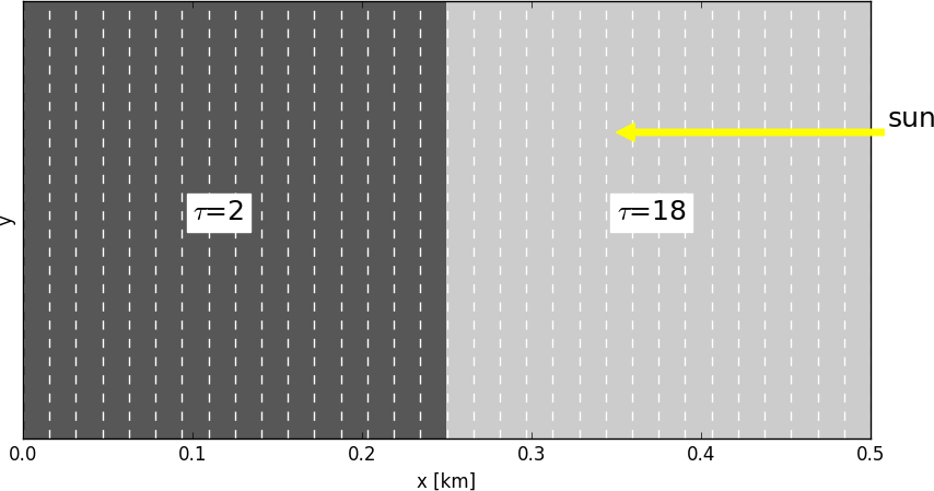
Figure 2: Definition of step cloud, test case C1. In x-direction the optical thickness of the cloud changes periodically between 2 and 18. In y-direction the cloud extends infinitely.

The first 16 pixels have an optical thickness $\tau$ of 2 and the remaining 16 pixels $\tau=$18. The size of the cloud field is 0.5 km and all pixels have a width of 0.5/32 km =15.625 m. The geometrical thickness of the cloud along the z-axis is 0.25 km and the cloud extends in y-direction infinitely. We assume periodical boundary conditions in x-direction (for Monte Carlo models this means that photons that leave the domain on one side of the domain at a certain vertical position re-enter the domain on the opposite side at the same vertical position without changing their propagation direction). Periodical boundary conditions are often used in Monte Carlo radiative transfer codes, because they ensure energy conservation and are appropriate for most applications, given that the model domain is sufficiently large so that the region of interest is not affected by the edge effects [Mayer, 2009]. The provided cloud optical properties were calculated using Mie theory for a wavelength of 800 nm using a gamma size distribution:

$$n(r)=Cr^{\alpha}\exp\left(-\frac{(\alpha+3)r}{r_{\rm eff}}\right)$$ (8)

Here $\alpha$ was set 7 and the effective radius $r_{\rm eff}$ was 10 $\mu$m. The effective variance is $v_{\rm eff}=\frac{1}{\alpha+3}=0.1$ which is a typical value for a liquid water cloud. The constant $C$ is obtained by normalization. The refractive index of water at 800 nm is 1.325+1.250$\cdot$10^-7 i [Segelstein, 1981], this means that there is almost no absorption. The surface albedo was set to 0 for this test case, i.e. we have a black surface corresponding to a water surface outside the sunglint region. The solar azimuth angle $\phi_{0}$ is 0^∘ (see also Figure 2).

Ten different sun-observer geometries as shown in Table 2 were calculated. Each geometry is defined by the solar zenith angle $\theta_{0}$, the solar azimuth angle $\phi_{0}$=0^∘, the altitude of the observer, the viewing zenith angle $\theta$ and the viewing azimuth angle $\phi$. The table also includes the scattering angle $\theta_{s}=\arccos({\bf n}_{0}\cdot{\bf n}_{v})$, where ${\bf n}_{0}$ is the sun position vector and ${\bf n}_{v}$ is the viewing direction vector. The angle between sun direction and viewing direction is the scattering angle $\theta_{s}$ for single scattering.

no.	$\theta_{0}$ [∘]	$z$ [km]	$\theta$ [∘]	$\phi$ [∘]	$\theta_{s}$ [∘]
1	0	0	60	0	60
2	60	0	0	0	60
3	60	0	30	0	30
4	60	0	30	180	90
5	0	0.25	180	0	180
6	0	0.25	140	0	140
7	0	0.25	120	0	120
8	60	0.25	180	0	120
9	60	0.25	120	0	60
10	20	0.25	120	135	132.8

Table 2: Geometrical settings for scenario C1 – step cloud. The solar azimuth angle is $\phi_{0}$=180^∘ for all cases.

For each of the directions we calculate the pixel averaged Stokes vector for all 32 pixels in the model domain. All Monte Carlo simulations were supposed to be run with 10⁷ “photons” per pixel, i.e. 32$\cdot$10⁷ photons in total. Two model runs with more photons were performed to obtain a reference. Table 3 includes more details about the settings of the Monte Carlo models. The MSCART model was run in forward tracing mode (MSCART-F) and backward tracing mode (MSCART-B). For SHDOM the number of discrete ordinates in zenith and azimuth angle were $N_{\mu}=64$ and $N_{\phi}$=128, and the spatial resolution was $N_{x}$=160 and $N_{z}$=81 for the base grid with cell splitting accuracy of 0.002.

model	$N_{ph}$	VR	TM
3DMCPOL	32$\cdot$107	no	F
SPARTA	32$\cdot$107	no	F
SPARTA 1011	1011	no	F
MSCART-F	32$\cdot$107	yes	F
MSCART-B	32$\cdot$107	yes	B
MYSTIC	32$\cdot$107	yes	F
MYSTIC-NV	32$\cdot$107	no	F
MYSTIC 32$\cdot$108	32$\cdot$108	yes	F

Table 3: Monte Carlo model settings for scenario C1 – step cloud. $N_{ph}$ is the number of photons, the VR column shows whether the models used variance reduction methods for spiky scattering phase functions and TM gives the tracing method (forward tracing (F) from the sun towards observer or backward (B) tracing from observer towards the sun).

4.2 C1 – Results

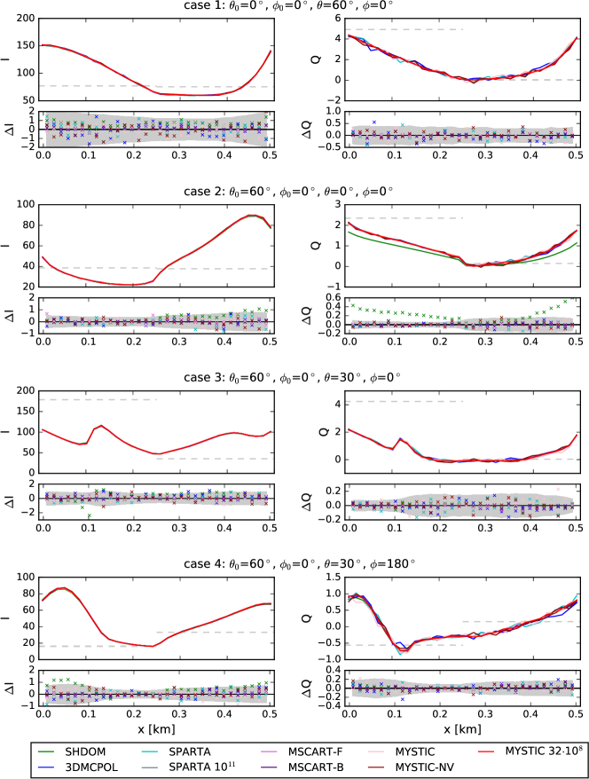
Figure 3: Stokes vector components $I$ (left) and $Q$ (right) for the step cloud scenario C1. Here, the observer is placed at the bottom of the cloud layer at position $x$ and it looks upwards, its viewing direction is given by ($\theta$,$\phi$). The solar zenith angle is 0^∘ for case 1 and 60^∘ for cases 2–4. The solar azimuth angle is 0^∘ for all cases. The small panels show the absolute differences between various models (see legend) and accurate MYSTIC simulations obtained with 10⁸ photons/pixel (MYSTIC 32$\cdot$10⁸). The grey range corresponds to 2$\sigma$ of MYSTIC simulations without variance reduction methods and with 10⁷ photons/pixel (MYSTIC-NV). The Stokes vector components are normalized to 1000/E₀. All cases are in the solar principal plane where the Stokes components $U$ and $V$ are exactly 0 and, therefore, not shown. The grey dashed lines show 1D independent pixel calculations.

Figure 3 shows the results for up-looking geometries (test cases 1–4). The observer is placed at the bottom of the cloud layer at position $x$ looking upwards. In the plots, the Stokes vector components are normalized to 1000/$E_{0}$, where $E_{0}$ corresponds to the extraterrestrial irradiance at the simulated wavelength (here 800 nm). The models generally produce the same spatial radiance patterns, meaning that they all handle horizontal photon transport correctly. The Monte Carlo models without variance reduction show significant noise in particular for $Q$ which is relatively small below the cloud.

Note that using a plane-parallel (1D) model and IPA, we would get only two different values in each of the plots, one from $x$=0 km to $x$=0.25 km where the optical thickness of the cloud is 2, and one from $x$=0.25 km to $x$=0.5 km where the optical thickness is 18. IPA results are included as grey dashed lines in the plots. Comparing them with the 3D results shows that in scenarios similar to the step cloud case, i.e. highly variable optical thickness on a small scale within the domain, it is important to consider horizontal photon transport, for the total radiance and also for the polarized radiance.

The small panels show the absolute differences between the model simulations (see legend) and accurate MYSTIC simulations obtained with 10⁸ photons/pixel (MYSTIC 32$\cdot$10⁸). The grey range corresponds to 2 standard deviations (2$\sigma$) of MYSTIC simulations without variance reduction methods and with 10⁷ photons/pixel (MYSTIC-NV), which corresponds to the default Monte Carlo model settings for this scenario. The differences for the Monte Carlo codes are within the expected 2$\sigma$ range. Some systematic deviations are found for the only deterministic code SHDOM: for case 2, where the sensor looks exactly into zenith direction, we see rather large deviations for Stokes component $Q$. The IPRT 1D intercomparison [Emde et al., 2015] showed a problem SHDOM has for Stokes components $Q$ and $U$ near $\theta$=0^∘ and $\theta$=180^∘ for highly peaked phase functions, and this issue has not yet been resolved.

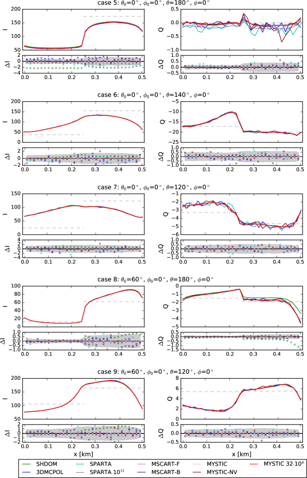
Figure 4: Stokes vector components I (left) and Q (right) for the step cloud scenario C1. Here the observer is placed at the top of the cloud layer at position x and it looks downwards and its viewing direction is given by ($\theta$,$\phi$). The solar zenith angle is 0^∘ for cases 5–7 and 60^∘ for cases 8–9. The solar azimuth angle is 0^∘ for all cases. The small panels show the absolute differences between various models (see legend) and accurate MYSTIC simulations obtained with 10⁸ photons/pixel (MYSTIC 32$\cdot$10⁸). The grey range corresponds to 2$\sigma$ of MYSTIC simulations without variance reduction methods and with 10⁷ photons (MYSTIC-NV). The Stokes vector components are normalized to 1000/E₀. All cases are in the solar principal plane where the Stokes components $U$ and $V$ are exactly 0 and, therefore, not shown. The grey dashed lines show 1D independent pixel calculations.

Figure 4 shows the results for down-looking geometries (test cases 5–9), where the observer is placed at the top of the cloud layer at position $x$ looking downwards. Again, we find generally a good agreement between all models, i.e. the differences are within the 2$\sigma$ range of MYSTIC-NV. There are only two obvious problems: (1) $Q$ for case 5, where the sensor looks exactly nadir and the sun is in zenith, is biased towards a negative value for SPARTA. (2) $Q$ for case 8, where the sensor also looks exactly nadir but the solar zenith angle is 60^∘, is positively biased for SHDOM.

As for the up-looking cases, models without variance reduction show significant noise, especially for case 5 and case 7, where $Q$ is very small.

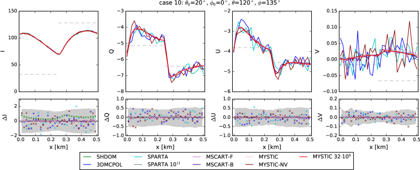
Figure 5: Stokes vector components I, Q, U, and V for the step cloud scenario C1. Here, the observer is placed at the top of the cloud layer at position x and it looks downwards and its viewing direction is given by ($\theta$=120^∘,$\phi$=135^∘). The solar zenith angle is $\theta_{0}$=20^∘ and the solar azimuth angle is $\phi_{0}$=0^∘. This sun-observer geometry is outside the solar principal plane and, hence, non-zero values for $U$ and $V$ are expected. The small panels show the absolute differences between various models (see legend) and accurate MYSTIC simulations obtained with 10⁸ photons/pixel (MYSTIC 32$\cdot$10⁸). The grey range corresponds to 2$\sigma$ of MYSTIC simulations without variance reduction methods and with 10⁷ photons (MYSTIC-NV). The Stokes vector components are normalized to 1000/E₀. The grey dashed lines show 1D independent pixel calculations.

Figure 5 shows the results for case 10, where the observer is placed at the top of the cloud layer at position $x$ looking downwards with viewing direction given by ($\theta$=120^∘,$\phi$=135^∘). The solar zenith angle is $\theta_{0}$=20^∘ and the solar azimuth angle is $\phi_{0}$=180^∘. This sun-observer geometry is the only one outside the solar principal plane, hence, we expect non-zero values for $U$ and $V$. The models generally agree within the 2$\sigma$ range of MYSTIC-NV. However, for $V$ the noise is very large and only models with variance reduction (MYSTIC and MSCART), or with a very large number of photon runs (SPARTA 10¹¹) produce a significant curve, where the noise is not larger than the values of $V$. The achieved accuracy of $V$ is consistent with García Muñoz [2015], who shows that 10⁹ photons or more are required to resolve circular polarization with values of $V/I$ of the order of 10^-5. A small bias in $I$ ($\Delta I/I\approx$0.5%) is seen for SHDOM.

In order to compare the models quantitatively, we calculate the statistical quantities as defined in Section 3.2. As reference model we have taken MYSTIC 32$\cdot$10⁸.

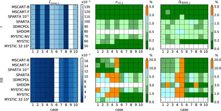
Figure 6: Statistics of Stokes vector components I and Q for the step cloud scenario C1. The left panels show the mean radiance (for Q the mean of the absolute values) for all models and all 10 cases. The middle panels show the standard deviations and the right panels show the root mean square differences $\Delta_{\rm RMS}$ in per cent. U and V are not shown here because they are 0 except for case 10.

Results are shown in Figure 6. The left panels show the mean radiances: rows correspond to the test cases 1–10 and columns correspond to results of the different models. We see a pattern of vertical lines which means that the mean radiances are approximately the same in all models. The middle plots show the mean relative standard deviations. For the default settings with 32$\cdot$10⁷ photons without using variance reduction methods (SPARTA, 3DMCPOL, MYSTIC-NV) $\sigma_{\rm rel,I}$ is between 0.2% and 1% (for the first Stokes component $I$). For up-looking cases 1–4, $\sigma_{\rm rel,I}$ is approximately the same for MYSTIC with and without variance reduction (MYSTIC-NV). This shows that for up-looking directions the variance reduction method VROOM [Buras and Mayer, 2011] as implemented in MYSTIC does not reduce the noise as expected and it should be optimized. For MSCART, $\sigma_{\rm rel,I}$ is below 0.2% for all cases in forward and backward tracing mode. It is also below 0.2% for the SPARTA run with 10¹¹ photons and the MYSTIC run with 32$\cdot$10⁸ photons, which is the expected result since $\sigma\propto N_{\rm ph}^{-1/2}$. For $Q$, the relative standard deviation is significantly larger because the mean values of $Q$ are 1-2 orders of magnitude smaller than $I$. For Monte Carlo runs with default settings, $\sigma_{\rm rel,Q}$ is between 1% and 10% for down-looking cases 6–10. For up-looking cases and case 5, the magnitude of $Q$ is very small and $\sigma_{\rm rel,Q}$ ranges from 5% to more than 20%. With variance reduction, $\sigma_{\rm rel,Q}$ is reduced to values below 1% for cases 5–10. The MSCART variance reduction method reduces $\sigma_{\rm rel,Q}$ to values below 3% also for up-looking directions. For $Q$, we also find that the MYSTIC variance reduction does not reduce the noise as expected for up-looking directions. SHDOM does not calculate standard deviations, thus the row corresponding to SHDOM results is left white.

The right panels show the relative RMS differences $\Delta_{\rm RMS,j}$. These should be similar to the $\sigma_{\rm rel,j}$ if the model results are not biased compared to the reference model. Indeed, we obtain similar values. For up-looking cases 1–4, $\Delta_{\rm RMS,Q}$ is larger than $\sigma_{\rm rel,Q}$ for the accurate models MSCART-F, MSCART-B and SPARTA 10¹¹, the reason for this is that the RMS difference is dominated by the less accurate reference calculation MYSTIC 32$\cdot$10⁸. For SHDOM, $\Delta_{\rm RMS,I}<$1% for all cases except 4 and 5, for those $\Delta_{\rm RMS,I}<$2%. $\Delta_{\rm RMS,Q}$ of SHDOM is smaller than the relative standard deviation of MYSTIC 32$\cdot$10⁸ for all cases except 2, 5, and 8, which are for either nadir or zenith viewing geometry.

5 Test case C2 – Cubic cloud

5.1 C2 – Model setup

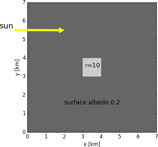
Figure 7: Definition of cubic cloud, test case C2.

The second test case includes a 1$\times$1$\times$1 km³ cubic cloud (see Figure 7). The domain size is 7$\times$7 km² in the x-y-plane and 5 km in z-direction. The cloud is located in the domain center: In x and y directions it extends from 3–4 km, respectively, and in z-direction it extends from 2–3 km. We assume periodic boundary conditions in x and y-directions. The vertical optical thickness of the cloud is 10 and, within the cube, the cloud extinction coefficient is constant. We use the same cloud optical properties as for the step cloud: a wavelength of 800 nm and and an effective droplet radius of 10 $\mu$m. Here, we assume that the cloud droplets do not absorb, i.e., the single scattering albedo was set to 1.0. We include a Lambertian surface with albedo 0.2 at the bottom of the domain. The solar azimuth angle is 180^∘, which means that the sun direction is along the x-axis (photons enter the atmosphere in positive x-direction). We calculate the polarized radiation fields with a spatial resolution of 70$\times$70 pixels for various viewing directions (see Table 4). Surface radiances are calculated for $\theta_{0}$ = 20^∘ and top-of-domain radiances for $\theta_{0}$ =40^∘. Table 4 also includes the scattering angle $\theta_{s}=\arccos({\bf n}_{0}\cdot{\bf n}_{v})$ for all of the 9 test cases.

no.	$\theta_{0}$ [∘]	$z$ [km]	$\theta$ [∘]	$\phi$ [∘]	$\theta_{s}$ [∘]
1	20	0	40	0	60.0
2	20	0	40	60	52.4
3	20	0	40	120	33.9
4	20	0	40	180	20.0
5	40	5	180	0	140.0
6	40	5	140	0	180.0
7	40	5	140	60	142.5
8	40	5	140	120	112.3
9	40	5	140	180	100.0

Table 4: Geometrical settings for cases C2 (cubic cloud) and C3 (cumulus cloud). The solar azimuth angle is $\phi_{0}$=180^∘ for all cases.

Two sets of simulations are performed: first, the cubic cloud is in vacuum and second, the cloud is included in a homogeneous Rayleigh scattering layer from 0 to 5 km with optical thickness set to 0.5 (this is a typical value at a wavelength of about 370 nm for the Earth atmosphere). The Rayleigh depolarization factor is set to 0. For the exact definition of the Rayleigh phase matrix, the reader is referred to Emde et al. [2015].

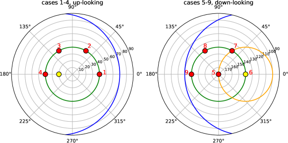
Figure 8: Viewing geometry for scenarios C2 (cubic cloud) and C3 (cumulus cloud). (Left panel:) up-looking directions (cases 1–4). The sun position (yellow circle) is $(\theta_{0},\phi_{0})=(20^{\circ},180^{\circ})$. The viewing zenith angle is constant (40^∘, green circle). The blue line corresponds to viewing directions with a scattering angle of 90^∘. (Right panel:) down-looking directions, cases 5–9. The sun in in the back from the perspective of the down-looking observer at the top of the atmosphere, i.e. the position vector of the sun is opposite to the viewing direction vector. The yellow circle at $(140^{\circ},0^{\circ})$ corresponds to the sun position $(\theta_{0},\phi_{0})=(40^{\circ},180^{\circ})$. The viewing angle is nadir for case 5 and 140^∘ otherwise (cases 6–9, green circle). The blue line shows viewing directions with a scattering angle of 90^∘ and the orange circle viewing directions with a scattering angle of 140^∘.

The viewing geometries are illustrated in Figure 8. The left plot shows the up-looking directions 1–4 and the right plot the down-looking directions 5–9. For up-looking directions in clear-sky regions, the highest degree of polarization is expected at a scattering angle of 90^∘ (blue line) because for this angle Rayleigh scattering causes the maximum degree of polarization of 100% for single scattering. Therefore, in the clear-sky region we expect decreasing polarization from case 1 to case 4. Also for down-looking directions we expect in clear-sky regions the highest degree of polarization at a scattering angle of 90^∘. Since case 9 is closest to the blue line, we expect for this case the highest polarization in the clear sky region. At a scattering angle of 140^∘ (orange line, cloud- or rainbow region), clouds cause high polarization, and therefore, in the cloudy region we expect the highest polarization for cases 5 and 7.

model	$N_{ph}$	VR	TM
3DMCPOL	49$\cdot$109	no	F
SPARTA	1$\cdot$1011	no	F
MSCART-F	49$\cdot$109	yes	F
MSCART-B	49$\cdot$109	yes	B
MYSTIC	49$\cdot$109	yes	F
MYSTIC-B	49$\cdot$109	yes	B

Table 5: Monte Carlo model settings for scenario C2 – cubic cloud. $N_{ph}$ is the number of photons, the VR column shows whether the models used variance reduction methods for spiky scattering phase functions and TM gives the tracing method (forward tracing (F) from the sun towards observer or backward (B) tracing from observer towards the sun).

The settings of the Monte Carlo models that have run the C2 cases are summarized in Table 5. Except SPARTA all have used the same number of photons (49$\cdot$10⁹) which corresponds to 10⁷ photons per pixel.

The SHDOM resolution parameters were $N_{\mu}$=32, $N_{\phi}$=64, $N_{x}$=140, $N_{y}$=140, $N_{z}$=101, and the cell splitting accuracy was 0.001. The factor of two reduction in angular resolution from case C1 was necessary due to the increased memory required by the 3D domain. Since most of the domain volume is occupied by vacuum or Rayleigh scattering, however, the SHDOM memory use is greatly reduced by the adaptive spherical harmonics truncation.

5.2 C2 – Results

We will discuss the results for three of the cases and show plots for all other cases in A.

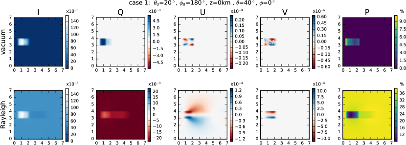
Figure 9: Results for scenario C2 (cubic cloud), case 1. The observer is at the ground and the viewing direction is $(\theta,\phi)=(40^{\circ},0^{\circ})$. The sun position is $(\theta_{0},\phi_{0})=(20^{\circ},180^{\circ})$. Upper panels: Cubic cloud is in vacuum. Lower panels: The cloud is embedded in a Rayleigh scattering layer. The labels on the x- and y-axes correspond to kilometers.

Figure 9 shows the MYSTIC results for case 1, where the observer is at the bottom. The viewing direction is $(\theta,\phi)=(40^{\circ},0^{\circ})$ and the sun position is $(\theta_{0},\phi_{0})=(20^{\circ},180^{\circ})$. In the upper panels the cubic cloud is in vacuum. The total radiance $I$ (upper left panel) shows that the cloud is illuminated from the left side. When the cloud is embedded in a Rayleigh scattering layer (lower panels) we see at the right of the cloud its shadow in the atmosphere. The polarization difference $Q$ caused by pure cloud scattering is positive in this geometry with a value of about 5$\cdot$10^-3 (radiance normalized to extraterrestrial irradiance at 800 nm). A positive $Q$ means that the radiation is polarized parallel to the scattering plane. The lower panel shows, that absolute value of $Q$ caused by Rayleigh scattering is much larger (about 20$\cdot$10^-3) and has a negative sign, thus Rayleigh scattering polarizes perpendicular to the scattering plane. The viewing direction is in the solar principal plane, i.e., $U$ and $V$ would be exactly 0 for 1D (IPA) radiative transfer calculations due to the symmetry. The cubic cloud breakes the symmetry and produces characteristic patterns in $U$ and $V$. At the cloud edge, the degree of polarization $P$ is up to 10% for the cloud in vacuum. Rayleigh scattering produces a $P$ of approximately 40% which is reduced inside the cloud and in the cloud shadow.

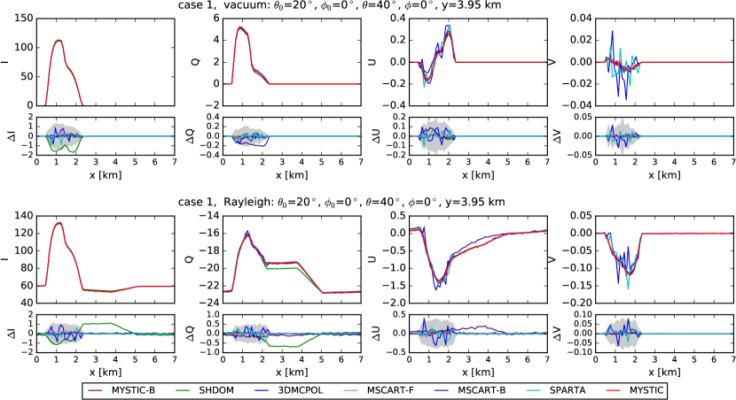
Figure 10: Results for scenario C2 (cubic cloud), case 1 for a cross section through the domain at y=3.95 km. The upper panels are for the cloud in vacuum and the lower panels for the cloud embedded in a Rayleigh scattering layer. The plots include the values of the Stokes components $I$, $Q$, $U$ and $V$, and below the absolute differences $\Delta I$, $\Delta Q$, $\Delta U$ and $\Delta V$ between the individual model results and MYSTIC. The grey area in the difference plots corresponds to 2$\sigma$ of 3DMCPOL (Monte Carlo model without variance reduction). The Stokes vector components are normalized to 1000/$E_{0}$.

The patterns which we see in Figure 9 look the same for all models. This is clearly seen in Figure 10, which shows all model results for a cross section through the model domain at y=3.95 km. We find quite large noise for Stokes components $U$ and $V$ for the models 3DMCPOL and SPARTA, but we see that those results lie in the range of the standard deviation of the 3DMCPOL model. We find small biases for SHDOM (green lines) and for MSCART-B, those will be further analysed below.

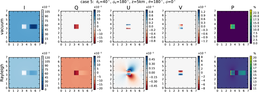
Figure 11: Results for scenario C2 (cubic cloud), case 5, for an observer at the top of the model atmosphere. The viewing direction is nadir and the sun position is $(\theta_{0},\phi_{0})=(40^{\circ},180^{\circ})$. Upper panels: Cubic cloud is in vacuum. Lower panels: The cloud is embedded in a Rayleigh scattering layer. The labels on the x- and y-axes correspond to kilometers.

Figure 11 shows the MYSTIC results for case 5, where the observer is at the top of the atmosphere. The viewing direction is nadir and the sun position is $(\theta_{0},\phi_{0})=(40^{\circ},180^{\circ})$. The total radiance $I$ shows the cubic cloud in the center of the domain as seen from above. Further, since the surface albedo is 0.2, we can clearly see the cloud shadow at the ground, which is shifted to the right. Cloud scattering and Rayleigh scattering both produce a negative $Q$ in this geometry. Since the scattering angle is 140^∘  the cloud produces a high degree of polarization of more than 25% and Rayleigh scattering about 15%. The degree of polarization in the cloud shadow is larger than the Rayleigh background because $I$ is small in the shadow. Again, we obtain patterns for $U$ and $V$, which are exactly 0 in the principal plane for 1D RT simulations.

Figure 12: Results for scenario C2 (cubic cloud), case 8. The sensor is at the top of the atmosphere and its viewing direction is $(\theta,\phi)=(140^{\circ},120^{\circ})$. The sun position is $(\theta_{0},\phi_{0})=(40^{\circ},180^{\circ})$. Upper panels: Cubic cloud is in vacuum. Lower panels: The cloud is embedded in a Rayleigh scattering layer. The labels on the x- and y-axes correspond to kilometers.

MYSTIC results for case 8 are shown in Figure 12, where the sun position is the same as for case 5. The sensor is at the top of the atmosphere with viewing direction $(\theta,\phi)=(140^{\circ},120^{\circ})$, i.e., outside the solar principal plane. Here, we expect larger values for $U$ which are indeed found in the results. For this geometry, $Q$ is positive for Rayleigh scattering and cloud scattering and $U$ is mostly negative, with a small positive area at the cloud edge. The degree of polarization is about 35% in the clear-sky region and about 20% in the cloud region. Due to periodic boundary conditions, the cloud shadow is shifted into the upper and lower left corner of the domain. The degree of polarization in the cloud shadow is about 45%.

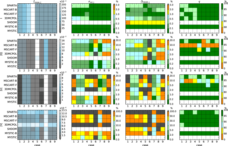
Figure 13: Statistics of the Stokes vector results for scenario C2 (cubic cloud in vacuum). The panels in the left column show the mean radiance $I_{\rm mean}$ (for Q, U, and V the mean of the absolute values) for all models and all 9 cases. The panels in the second column show the standard deviations $\sigma_{\rm rel}$. The third column shows the root mean square differences $\Delta_{\rm RMS}$ with respect to MYSTIC in per cent and the right column shows the match fractions $q$.

Figure 13 shows the statistics of the model results for the cubic cloud in vacuum. All quantities were calculated according to the definitions in Sec. 3.2. The mean radiance $I_{mean}$ (panels in left column) is very similar for all models and all cases for the Stokes components $I$, $Q$ and $U$.

For the circular polarization component $V$, which is about three orders of magnitude smaller than $Q$ and $U$ we find significant differences. In particular, $I_{\rm mean,V}$ is larger for SPARTA and 3DMCPOL compared to other models. The reason is that those two models have not used variance reduction methods so that $\sigma_{\rm rel,V}$ is larger than the absolute value of $V$. The second column shows, that $\sigma_{\rm rel,V}$ is more than 100% for SPARTA and 3DMCPOL for all cases except case 7. Also, other models show very large noise for $V$; the only case with $\sigma_{\rm rel,V}$ smaller than 30% is case 7, where the mean value of $I_{\rm mean,V}$ is the largest.

For the first Stokes component (upper row in Figure 13), $\sigma_{\rm rel,I}$ of all Monte Carlo codes is below 0.1% for down-looking directions (cases 5–9). For up-looking directions (cases 1–4) $\sigma_{\rm rel,I}$ is slightly larger for the models SPARTA and 3DMCPOL but still below 1%. The root mean square difference $\Delta_{\rm RMS,I}$ is similar to $\sigma_{\rm rel,I}$ for all cases and all Monte Carlo models. For SHDOM we obtain $\Delta_{\rm RMS,I}$ values of about 1–2%, because SHDOM uses a different method to solve the VRTE, in particular also a different grid discretization. The match fraction $q_{I}$ is mostly larger than 95%, i.e., the models agree within the Monte Carlo noise. For up-looking cases, we often find values between 90% and 95%, which means that the number of matches is slightly smaller than the expected assuming Gaussian statistics. This can be explained by the small number of contributing pixels ($N_{\rm all}$ $\approx$200), because in the up-looking geometry only pixels within the cloud have radiance values different from 0. For SHDOM, we do not include a match fraction because SHDOM does not calculate a standard deviation since it applies a deterministic method.

For SHDOM, $\Delta_{\rm RMS,I}$ is mostly about 1–2%; $\Delta_{\rm RMS,Q}$ and $\Delta_{\rm RMS,U}$ are in the range from 1–20%, with larger values for down-looking directions.

The plots of $\sigma_{\rm rel,Q}$ and $\sigma_{\rm rel,U}$ show, that the variance reduction methods included in MYSTIC and in MSCART work very well and reduce the relative standard deviation from values between 2-5% to values below 1% for a given number of photons. We find that MSCART-B (backward tracing mode) disagrees to the other models, as the match fractions $q_{Q}$ and $q_{U}$ are almost always smaller than 90%. The main reason for this discrepancy arises from the invalidation of the reciprocity principle when using a scattering-order-dependent phase function truncation approximation [Wang et al., 2017, Iwabuchi and Suzuki, 2009] in backward tracing mode. For the backward simulation with this kind of truncation approximation, the truncation fraction gradually increase with decreasing scattering order, since the photons are traced from detector (corresponding to the last order) to source (corresponding to the first order). This means that, for the nth-order radiance estimation, the greatest truncation occurs at the first-order scattering simulation while the smallest one at the nth-order. The scattering-order-dependent phase function truncation approximation produces a bias which is small for forward tracing and can become larger in backward tracing mode.

For MYSTIC, which aplies the variance reduction methods VROOM [Buras and Mayer, 2011], we obtain the same results in forward and in backward tracing mode (MYSTIC-B).

For several cases $\sigma_{\rm rel,Q}$, $\sigma_{\rm rel,U}$, $\Delta_{\rm RMS,Q}$ and $\Delta_{\rm RMS,U}$ are larger than 20%. These are the cases where the polarized radiance values are very small. The dark grey values in the plots for $I_{Q}$ and $I_{U}$ are values below 10^-4, thus a relative standard deviation or relative root mean square error is not meaningful for these cases. The mean radiance $I_{V}$ is always smaller than 10^-5, therefore $\sigma_{\rm rel,V}$ and $\Delta_{\rm RMS,V}$ are always large and a quantitative comparison for circular polarization is not possible.

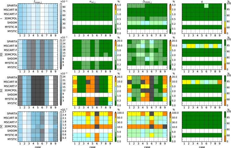
Figure 14: Statistics of the Stokes vector results for scenario C2 (cubic cloud in Rayleigh layer). The panels in the left column show the mean radiance $I_{\rm mean}$ (for $Q$, $U$, and $V$ the mean of the absolute values) for all models and all 9 cases. The panels in the second column show the standard deviations $\sigma_{\rm rel}$. The third column shows the root mean square differences $\Delta_{\rm RMS}$ with respect to MYSTIC in per cent and the right column shows the match fractions $q$.

The statistics for the cubic cloud embedded in a Rayleigh scattering layer is shown in Figure 14. Generally, the results become more accurate than for the cloud in vacuum, because Rayleigh scattering is not characterized by strongly peaked scattering phase functions as cloud scattering. Monte Carlo models can accurately simulate Rayleigh scattering for relatively thin planetary atmospheres such as the Earth’s atmosphere without variance reduction methods. However, García Muñoz and Mills [2015] show that for optically thick planetary atmospheres with strong Rayleigh scattering ($\tau$=16) the directional sampling as implemented e.g. in MYSTIC [Emde et al., 2010] causes numerical problems so that the results do not converge. To overcome this problem they developed the “pre-conditioned backward Monte Carlo” method which yields convergent results also for optically thick planetary atmospheres.

The standard deviation $\sigma_{\rm rel,I}$ is generally smaller than 0.1%, $\sigma_{\rm rel,Q}$ and $\sigma_{\rm rel,U}$ are smaller than 1% for all cases with mean values of $I_{\rm mean,j}$ larger than approximately 3$\cdot$10^-3. As for the cloud in vacuum, MSCART in backward tracing mode yields significantly deviating results for $Q$ and $U$, whereas in forward tracing mode it agrees perfectly to the other codes. For SPARTA we find a significant difference for $I$ (case 6). For SHDOM $\Delta_{\rm RMS,I}$, $\Delta_{\rm RMS,Q}$, and $\Delta_{\rm RMS,U}$ are smaller than 1%.

Figure 15: Absolute differences for Stokes vector components $I$, $Q$, $U$, $V$, and the degree of polarization $P$ between individual model results and MYSTIC ($I_{i,model}-I_{i,MYSTIC}$) for cubic cloud in Rayleigh layer (C2), case 6. Each row corresponds to a different model, see labels on the left. The labels on the x- and y-axes correspond to kilometers.

To further analyze model discrepancies, we show the absolute differences between MYSTIC and individual model results for case 6 in Figure 15. Case 6 (direct backscattering) is the most problematic case which shows discrepancies for SHDOM, SPARTA, and MSCART-B. The limits of the colorbars in the figure are set to 5% of the maximum value of the MYSTIC results for $I$ and $P$, and to 10% of the MYSTIC results for $|Q|$ and $|U|$. Values larger than the upper limit are marked in purple and values smaller than the lower limit are marked in green.

The differences between MYSTIC and MYSTIC-B show only statistical noise according to the standard deviations of the results, thus MYSTIC obtains the same results in forward tracing and backward tracing mode, as expected.

In direct backscattering geometry, SHDOM gives lower accuracy using the TMS radiance method [Evans, 1998] due to the finely structured glory peak of the cloud phase function. The systematic differences between SHDOM and MYSTIC results are the following: For $I$, SHDOM obtains slightly smaller values than MYSTIC outside the cloud and larger values inside the cloud. On the cloud boundary, SHDOM results are also smaller than MYSTIC. Inside the cloud, $Q$ obtained with SHDOM is larger than MYSTIC. The larger $Q$ value within the cloud results in a larger degree of polarization $P$; it is about 0.1% larger for SHDOM compared to MYSTIC.

The difference between 3DMCPOL and MYSTIC exhibits a tiny negative bias in the cloud area for $I$. All other Stokes components and also $P$ show only statistical noise and no systematic differences. MSCART-F agrees perfectly to MYSTIC, only statistical noise is visible in the difference plots. MSCART-B shows obvious systematic differences for $U$ and $V$, and thus, in $P$. These differences are probably due to the variance reduction method in MSCART (see explanation above). For SPARTA there is a tiny negative bias in the cloud region for $I$ and a larger negative bias for $Q$, which becomes visible also in the difference plot for $P$.

In summary, we may conclude that, with a few exceptions, the models MSCART-F, MYSTIC, MYSTIC-B, 3DMCPOL, and SPARTA, yield equal results for the cubic cloud scenario in vacuum and in a Rayleigh scattering atmosphere. “Equal results” means that the differences between the models is smaller than two standard deviations for more than 96% of the calculated pixels. SHDOM results have larger $\Delta_{\rm RMS}$ than the Monte Carlo codes mainly due to the inherently lower angular and spatial resolution of a deterministic representation code. MSCART-B produces significant biases in $Q$ and $U$ for the setup including the cubic cloud.

6 Test case C3 – Cumulus cloud field

6.1 C3 – Model setup

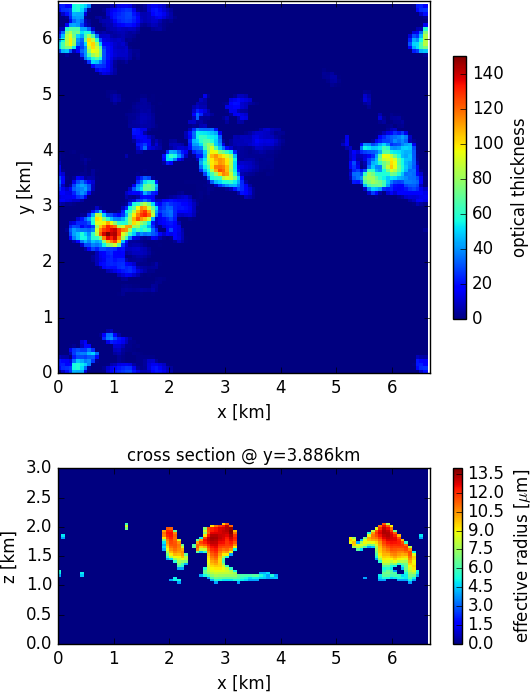
Figure 16: Definition of cumulus cloud, test case C3.

This test case includes a shallow cumulus cloud field from large-eddy simulations (LES) by Stevens et al. [1999], the same field was also used in the I3RC (Intercomparison of 3D radiation Codes) project [Cahalan et al., 2005]. The cloud field consists of 100$\times$100$\times$36 grid cells with a size of 66.7$\times$66.7$\times$40 m³. Extinction coefficients and effective droplet radii for each grid cell were provided as model input data. The upper panel in Figure 16 shows the vertically integrated optical thickness of the clouds and the lower panel shows the effective radius for a vertical cross section at y = 3.886 km. As for the cubic cloud case (C2), two sets of simulations were performed at a wavelength of 670 nm. In the first set of simulations, the cloud field is embedded in a molecular atmosphere; altitude profiles of molecular absorption coefficients and Rayleigh scattering coefficients were given as input for all models. The Rayleigh depolarization factor was set to 0. The second set of simulations additionally includes aerosols; the altitude profile of aerosol extinction coefficients were also provided as model input. Figure 17 shows altitude profiles of absorption and scattering coefficients of molecules and aerosols.

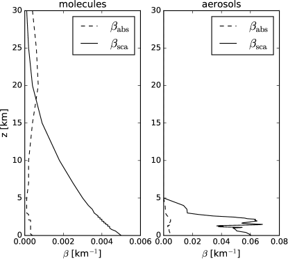
Figure 17: Altitude profiles of absorption coefficients $\beta_{\rm abs}$ and scattering coefficents $\beta_{\rm sca}$ coefficients for molecules (left) and aerosols (right). These profiles were used as atmospheric background for the simulations of the shallow cumulus field C3.

Aerosol and cloud optical properties were precalculated using Mie theory and provided as model input. For aerosols, we used the refractive index and size distribution parameters for water soluble aerosol from the OPAC database [Hess et al., 1998]. The single scattering albedo is approximately 0.93. A Lambertian surface was included with albedo 0.2 and, as for scenario C2, the solar azimuth angle is 180^∘ in all test cases. Output altitudes, solar zenith angles and viewing directions are the same as for scenario C2 (see Table 4).

model	$N_{ph}$	VR	TM
3DMCPOL	1010	no	F
SPARTA	1010	no	F
MSCART-F	1010	yes	F
MSCART-B	1010	yes	B
MYSTIC	1010	yes	F

Table 6: Monte Carlo model settings for scenario C3 – cumulus cloud field. $N_{ph}$ is the number of photons, the VR column shows whether the models used variance reduction methods for spiky scattering phase functions and TM gives the tracing method (forward tracing (F) from the sun towards observer or backward (B) tracing from observer towards the sun).

Table 6 shows the settings of the Monte Carlo models that have run the C3 test cases with the cumulus cloud field. For these test cases all models have run the commonly agreed number of photons of 10¹⁰ which corresponds to 10⁶ photons per pixel. Since the number of photons per pixel is a factor of 10 smaller than for test cases C2, we expect less accurate results (the standard deviation is expected to increase by a factor of $\sqrt{10}$). The SHDOM resolution parameters were $N_{\mu}=16$, $N_{\phi}$=32, $N_{x}$=100, $N_{y}$=100, $N_{z}$=55, and cell splitting accuracy of 0.03. The further reduction of the angular and spatial resolution from case C2 was required by the large domain filled with aerosols, for which the adaptive spherical harmonics truncation does not save significant memory.

6.2 C3 – Results

In this section we will discuss the results for three of the cases, plots of all other cases are shown in A.

Figure 18: Results for scenario C3 (shallow cumulus cloud field), case 2, for an observer at the surface. The viewing direction is $(\theta,\phi)=(40^{\circ},60^{\circ})$ and the sun position is $(\theta_{0},\phi_{0})=(20^{\circ},180^{\circ})$. Upper panels: The cumulus cloud field is surrounded by a molecular atmosphere. Lower panels: Aerosol is added to the scenario. The labels on the x- and y-axes correspond to kilometers.

Figure 18 includes the MYSTIC results for case 2, where the observer is placed at the surface, viewing upwards into direction $(\theta,\phi)=(40^{\circ},60^{\circ})$. The sun position is $(\theta_{0},\phi_{0})=(20^{\circ},180^{\circ})$. The plot nicely shows that the clouds are illuminated from the bottom-left side in this geometry. The upper plots are for the clouds embedded in a pure molecular atmosphere. $Q$ is negative in the clear-sky region and $U$ is positive. Inside the clouds, $Q$ and $U$ have opposite signs or the polarization becomes close to 0. For the circular polarization $V$, we see clear patterns with negative values on the left hand side of the sun direction and positive values on the right hand side. The degree of polarization is about 30% in the clear sky region and very small inside the clouds.

The bottom plots are for the same molecular atmosphere, but including aerosol in addition. We see in the $Q$ and $U$ plots that aerosol produces the same signs as Rayleigh scattering, thus it enhances the polarized radiance. The pattern in $V$ remains the same as without aerosol, but the magnitude is larger and the Monte Carlo noise becomes smaller. The degree of polarization is similar with and without aerosol, because as $Q$, $U$, and $V$ are increased by aerosol scattering, also the intensity $I$ is increased.

Figure 19: Results for scenario C3 (shallow cumulus cloud field), case 7, for an observer at the top of the model atmosphere. The viewing direction is $(\theta,\phi)=(140^{\circ},60^{\circ})$ and the sun position is $(\theta_{0},\phi_{0})=(40^{\circ},180^{\circ})$. Upper panels: The cumulus cloud field is surrounded by a molecular atmosphere. Lower panels: Aerosol is added to the scenario.The labels on the x- and y-axes correspond to kilometers.

Figure 19 shows the MYSTIC results for case 7. Here, the observer is at the top of the atmosphere and looks into direction $(\theta,\phi)=(140^{\circ},60^{\circ})$. The sun direction is $(\theta_{0},\phi_{0})=(40^{\circ},180^{\circ})$. Figure 8 shows that in this geometry the scattering angle is 140^∘, therefore we expect that the clouds generate polarization because we know that the cloud-bow is polarized. The $Q$ and $U$ plots nicely show the polarization by cloud scattering. $Q$ and $U$ are both positive and the values inside the cloudy region are much larger than the background. For aerosol, the background polarization is slightly larger, but still it is much smaller than the polarization by cloud scattering. For $V$, we see again symmetric patterns about the sun direction. The degree of polarization in the clouds is roughly between 10% and 20%, where the highest values are obtained for thin clouds, e.g., the small cloud at around $x$ =6.2km and $y$ =4.2km. In the image of the radiance $I$, it appears relatively faint, whereas in the image of the degree of polarization $P$ it is one of the brightest spots. The degree of polarization in the thick clouds becomes very small due to multiple scattering, which increases $I$, but not $Q$, $U$, and $V$ by the same magnitude, because $Q$, $U$ and $V$ saturate after a few scattering orders. The degree of polarization in the cloud shadows is increased because $I$ is decreased.

Figure 20: Results for scenario C3 (shallow cumulus cloud field), case 7, for a cross section through the domain at y=2.03 km. The upper panels are for the cloud in vacuum and the lower panels for the cloud embedded in a Rayleigh scattering layer. The plots include the values of the Stokes components $I$, $Q$, $U$ and $V$, and below the absolute differences $\Delta I$, $\Delta Q$, $\Delta U$ and $\Delta V$ between the individual model results and MYSTIC. The grey area in the difference plots corresponds to 2$\sigma$ of 3DMCPOL (Monte Carlo model without variance reduction). The Stokes vector components are normalized to 1000/$E_{0}$.

Figure 20 shows the results of all models for a cross section though the model domain at y=2.03 km. For all Monte Carlo codes, the results are very similar for $I$, $Q$, and $U$. For $V$ the noise is much larger than the value of $V$ for models without variance reduction methods (SPARTA, 3DMCPOL). For all Stokes components differences between the Monte Carlo models and MYSTIC are within the grey area defined by two standard deviations of 3DMCPOL. SHDOM results show the same spatial patterns but are slightly biased against the Monte Carlo results. This will be further discussed below.

Figure 21: Results for scenario C3 (shallow cumulus cloud field), case 9, for an observer at the top of the model atmosphere. The viewing direction is $(\theta,\phi)=(140^{\circ},180^{\circ})$ and the sun position is $(\theta_{0},\phi_{0})=(40^{\circ},180^{\circ})$. Upper panels: The cumulus cloud field is surrounded by a molecular atmosphere. Lower panels: Aerosol is added to the scenario. The labels on the x- and y-axes correspond to kilometers.

Figure 21 shows the MYSTIC results for case 9. The observer is placed at the top of the atmosphere and its viewing direction is $(\theta,\phi)=(140^{\circ},180^{\circ})$. The sun position is $(\theta_{0},\phi_{0})=(40^{\circ},180^{\circ})$. In this geometry with a scattering angle of 80^∘, we expect polarization from Rayleigh and aerosol scattering. Since we are in the solar principal plane, the mean of $U$ and $V$ should be close to 0. We obtain negative values of $Q$ from molecular scattering. Also, clouds produce negative $Q$ polarization in this geometry, so the clouds show higher absolute $Q$-values than the background in particular on the side facing the sun. The degree of polarization is about 5% in the clear-sky region. When aerosol particles are added, the background becomes much more polarized with negative $Q$-values. The degree of polarization increases to about 25%. The absolute value of $Q$ is now larger in the clear-sky region with aerosols than within the clouds.

Figure 22: Statistics of the Stokes vector results for scenario C3 (cumulus cloud field in molecular atmosphere). The panels in the left column show the mean radiance $I_{\rm mean}$ (for Q, U, and V the mean of the absolute values) for all models and all 9 cases. The panels in the second column show the standard deviations $\sigma_{\rm rel}$. The third column shows the root mean square differences $\Delta_{\rm RMS}$ in per cent and the right column shows the match fractions $q$.

Figure 22 shows the statistics for the cumulus cloud field in the molecular atmosphere. The mean radiance $I_{\rm mean,I}$ is very similar for all models. The mean values $I_{\rm mean,Q}$, $I_{\rm mean,U}$, and $I_{\rm mean,V}$ show several differences: As for the cubic cloud scenario C2 (Section 5.2), $I_{\rm mean,V}$ is significantly larger for SPARTA and 3DMCPOL than for the other models, because the accuracy is lower for models without variance reduction techniques. The mean values $I_{\rm mean,U}$ are smaller than 10^-4 for cases 1,4,5,6, and 9 (dark grey). For all these cases, $\sigma_{\rm rel,U}$, $\Delta_{\rm RMS,U}$, and $q_{U}$ are not meaningful. For case 6, the same applies for $I_{\rm mean,Q}$.

The values of $\sigma_{\rm rel,I}$ are always below 2% for SPARTA and 3DMCPOL. For MSCART-F and MSCART-B, $\sigma_{\rm rel,I}$ is below 0.5%. For MYSTIC $\sigma_{\rm rel,I}$ is smaller than 0.5% for down-looking cases 5–9 and between 0.5% and 1% for up-looking directions. This demonstrates once more that the variance reduction method VROOM reduces the noise better for down-looking than for up-looking directions.

The relative standard deviations $\sigma_{\rm rel,Q}$ and $\sigma_{\rm rel,U}$ are below 5% for models with variance reduction and cases where the $I_{\rm mean,Q}$ and $I_{\rm mean,U}$ are larger than approximately 10^-3.

The match fraction $q$ is larger than 95% for most cases. Obvious differences are only found for cases 2, 3, and 5 for the SPARTA model, where $q_{Q}$ and $q_{U}$ are smaller than 95%. Further for cases 8 and 9, $q_{I}$ is smaller than 95% for MSCART-B; for case 6, $q_{I}$ is smaller than 95% for SPARTA.

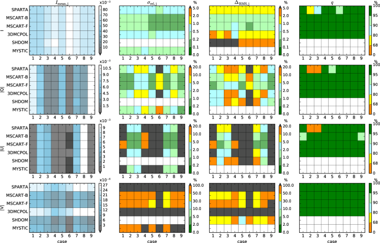
Figure 23: Statistics of the Stokes vector results for scenario C3 (cumulus cloud field and aerosol in molecular atmosphere). The panels in the left column show the mean radiance $I_{\rm mean}$ (for Q, U, and V the mean of the absolute values) for all models and all 9 cases. The panels in the second column show the standard deviations $\sigma_{\rm rel}$. The third column shows the root mean square differences $\Delta_{\rm RMS}$ in per cent and the right column shows the match fractions $q$.

Figure 23 shows the statistics for the cumulus cloud field in the molecular atmosphere containing aerosols. The mean values of the Stokes vector (left column) are similar for all models.

The relative standard deviations $\sigma_{\rm rel,I}$ are below 0.5% for MSCART-B, MSCART-F, and MYSTIC. Only for case 4, $\sigma_{\rm rel,I}$ for MYSTIC is between 0.5% and 1%. MSCART-F and MSCART-B yields the smallest values ($\sigma_{\rm rel,I}$$<$0.2%) for the down-looking cases 5–9 which demonstrates that for cases with aerosol and clouds, the variance reduction method of MSCART is more efficient than VROOM. Also, $\sigma_{\rm rel,Q}$ and $\sigma_{\rm rel,U}$ are often below 1% for MSCART-F and MSCART-B, for MYSTIC the values are between 1% and 2%. The accuracy of SPARTA and 3DMCPOL is lower, $\sigma_{\rm rel,I}$ is mostly between 0.5% and 1%; $\sigma_{\rm rel,Q}$ and $\sigma_{\rm rel,U}$ are in the range from 2% to 5% for mean values of $I_{\rm mean,Q}$ and $I_{\rm mean,U}$ larger than about 10^-3.

The $\Delta_{\rm RMS}$ values are generally larger than $\sigma_{\rm rel}$  because they include the inaccuracies of the two models that are compared. For SHDOM, $\Delta_{\rm RMS,I}$ is larger than for all Monte Carlo codes with values between 2% and 5% for all down-looking cases 5–9, and more than 5% for the up-looking cases. For $Q$ and $U$, the $\Delta_{\rm RMS}$-differences of SHDOM are comparable to those of SPARTA and 3DMCPOL.

For circular polarization, $\sigma_{\rm rel,V}$ and $\Delta_{\rm RMS,V}$ are generally very high. Values below 100% are obtained only for MSCART-F, MSCART-B, and MYSTIC. The $\Delta_{\rm RMS,V}$-difference between MSCART-F, MSCART-B, and MYSTIC is comparable to the $\Delta_{\rm RMS,V}$-difference between SHDOM and MYSTIC.

The match fraction $q$ reveals problems for SPARTA, mainly for test cases 2 and 3. Smaller differences for SPARTA also exist for case 5 (see $q_{Q}$) and case 6 (see $q_{I}$). Further we again see a small deviation for MSCART-B for cases 1 and 9 for the $U$-component. However, for these cases the mean value of $I_{\rm mean,U}$ is smaller than 10^-4, thus these differences are not meaningful.

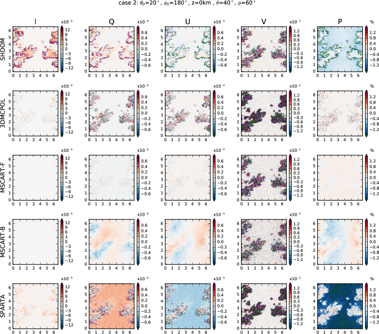
Figure 24: Absolute differences between individual model results and MYSTIC ($I_{i,model}-I_{i,MYSTIC}$) for the cumulus cloud field in a molecular atmosphere with aerosols included (C3), case 2. Each row corresponds to a different model, see labels on the left. The labels on the x- and y-axes correspond to kilometers.

In order to investigate the reasons for differences revealed in the statistics, we show the absolute differences between MYSTIC and individual model results for case 2 in Figure 24. The limits of the colorbar are set to 5% of the maximum value of the MYSTIC results for $I$ and $P$ and to 10% of the MYSTIC result for $|Q|$ and $|U|$. Values larger than the upper limit are marked in purple and values smaller than the lower limit are marked in green.

SHDOM shows the largest differences at the cloud boundaries as expected. But also the background shows systematic differences: the degree of polarization obtained with SHDOM is smaller than MYSTIC.

For 3DMCPOL the difference plots show only statistical noise, which is of course larger in the cloud regions than in clearsky regions.

Also MSCART-F agrees perfectly to MYSTIC. Compared to 3DMCPOL, we find much less noise because MSCART-F applies variance reduction methods. For MSCART-B we find systematic differences for $Q$ and $U$ (inside the cloud regions MYSTIC results are larger and outside the clouds MSCART-B results are larger). These differences can again be attributed to the variance reduction method of MSCART, which introduces a bias in backward tracing mode.

For SPARTA significant differences are found in particular in the clear-sky region for $Q$ and $U$. The reason for these differences could not be explained so far. It should be noted again, that the differences occur only for a few specific geometries.

In summary, we find a good agreement between the Monte Carlo models for the cumulus cloud scenario. Obvious differences for a few of the cases have been found between SPARTA and the other models, those should be further investigated. SHDOM radiances are somewhat biased relative to those of the Monte Carlo codes due to the lower angular resolution, and the differences are larger on the cloud boundaries due to interpolating the optical properties between grid points instead of assuming uniform cells as for the Monte Carlo codes.

7 Summary and Outlook

We have presented the IPRT radiative transfer model intercomparison for polarized radiative transfer in 3D geometry. Five models participated; four of them (3DMCPOL, MSCART, MYSTIC, and SPARTA) apply the Monte Carlo method to solve the vector radiative transfer equation, one uses the spherical harmonics discrete ordinate method (SHDOM).

The first series of test cases are based on a simple two dimensional step cloud with an optical thickness of 2 in one half and optical thickness of 18 in the other half. We simulated various sun-observer geometries, with sensor positions below the cloud and above the cloud. The results of this test demonstrate, that the polarized radiance is significantly influenced by horizontal photon transport. Generally we find a very good agreement between the models within the expected accuracy determined by the standard deviation of the Monte Carlo results. We compared results obtained with the same number of photons and tested the performance of variance reduction techniques as included in MYSTIC and MSCART. For down-looking directions the standard deviation is similar in the two models, for up-looking directions, the MYSTIC variance reduction method VROOM is less efficient. Apart from two exceptions for specific geometries, where the model SHDOM shows significant deviations, the models agree perfectly within the statistical noise. As reference, MYSTIC has been run with 10 times more photons. The relative standard deviation of the reference simulation is below 0.2% for $I$, below 1% for $Q$ and $U$ for down-looking direction, and below 5% for $Q$ and $U$ for up-looking directions.

The second series of test cases are based on a single cubic cloud with an optical thickness of 10. The first set of simulations are for the cubic cloud in vacuum. Of particular interest are simulations in the solar principal plane, for which the Stokes vector components $U$ and $V$ are exactly 0 in 1D plane-parallel geometry. The limited extension of the cloud breaks the symmetry between left side and right side of the solar principal plane and characteristic polarization patterns are generated. Furthermore it is interesting to see, how the polarization changes with the sun-observer geometry. In the second set of simulations, the cubic cloud is surrounded by a Rayleigh scattering layer with an optical thickness of 0.5. Here the results show, how the polarization caused by cloud scattering propagates in the clear-sky (Rayleigh scattering) part. Both cases show that plane-parallel radiative transfer, which would result in only two values, one for the cloud and one for the surrounding, can only be a rough approximation. We have found a good quantitative agreement between the Monte Carlo codes. MSCART agrees well to the other codes in forward tracing mode but shows a significant bias in backward tracing mode, which can most probably be attributed to the scattering-order dependent truncation method used by MSCART. SPARTA deviates significantly for a few geometries, the reason for this has not yet been found. SHDOM shows overall the same patterns as the Monte Carlo models, but the $\Delta_{\rm RMS}$ are larger than for the Monte Carlo codes mainly due to the inherently lower angular and spatial resolution of a deterministic representation code. We again use the MYSTIC results as reference because they are accurate and the variance reduction method is unbiased. The achieved accuracy (relative standard deviation of MYSTIC results) is of the order of 0.1% for the unpolarized radiance $I$ and of the order of 1% for polarized radiance $Q$ and $U$. For $V$, the accuracy is much less (more than 10%) but still the characteristic patterns could be compared qualitatively for models with variance reduction and SHDOM and they were found to look identical.

The third series of test cases, the most realistic scenarios, are based on a LES cloud field which is surrounded by a standard molecular atmosphere. A first set of simulations is without aerosols, in a second set a realistic aerosol optical thickness profile is added. Due to computational time limitations, the simulations were performed with 10 times less photons per pixel compared to the cubic cloud cases. We found generally a good agreement between the Monte Carlo codes. MSCART-B polarized radiance results exibit a bias also for the LES cloud field, which is smaller than in the cubic cloud case. SHDOM shows the same patterns as the Monte Carlo codes, but the quantitative comparison reveals differences particularly on cloud and cloud shadow boundaries. As for the cubic cloud case, SPARTA deviates from the other codes for a few specific cases including the LES clouds. The MYSTIC results, which were taken as reference, achieve an accuracy (relative standard deviation) of the order of 0.5%-1% for the unpolarized radiance $I$ and of the order of 5% for the polarized radiance $Q$ and $U$. For $V$, the relative standard deviation is in the range from 50%–100% for the cases with aerosols, without aerosols even larger. Still, the characteristic patterns are clearly visible and can be used for qualitative comparisons with other models.

We have not compared the computational times, because all simulations were performed on different computation clusters, thus we can not decide, which of the methods is the most efficient one. The computational time of a Monte Carlo simulation depends on the required accuracy, because the standard deviation of the result is proportional to $1/\sqrt{N_{\rm ph}}$. It also depends on the spatial resolution: in order to simulate an image of e.g. 100$\times$100 pixels we need 10000 times more photons than to simulate the domain average radiance for the same scene for a given accuracy. Furthermore, the CPU time depends on the average optical thickness of the scene, which determines the amount of multiple scattering. Roughly estimated, the computational times to reach a relative standard deviation of about 1% or less for the Stokes components $I$, $Q$, and $U$ vary from about 10 seconds per pixel for the cubic cloud case to about 5 minutes per pixel for the step cloud and the cumulus cloud scene. These times refer to MYSTIC simulations with variance reduction on one processor (Intel(R) Xeon(R) CPU E5-2630 v4 @ 2.20GHz).

The results of all models are available on the IPRT webpage (http://www.meteo.physik.uni-muenchen.de/~iprt) and the supplementary material to this publication includes MYSTIC results of cases. The webpage also provides detailed descriptions of all test cases including the required input data.

IPRT has planned two further intercomparison projects: one will focus on polarized radiative transfer in spherical geometry, the other one on multiple-scattering lidar simulations.

Appendix A Plots of the results of all testcases including cubic cloud (C2) and cumulus clouds (C3)

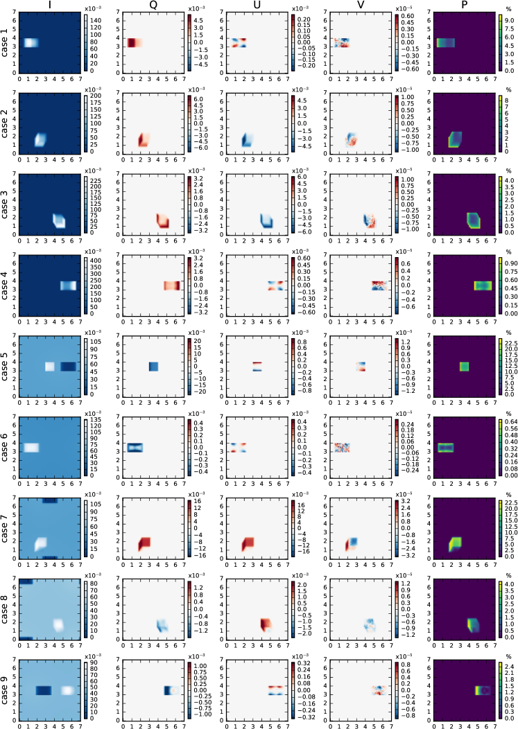
Figure 25: Results for scenario C2 (cubic cloud in vacuumn).

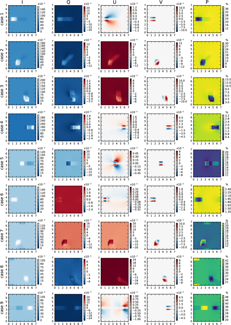
Figure 26: Results for scenario C2 (cubic cloud in Rayleigh scattering layer).

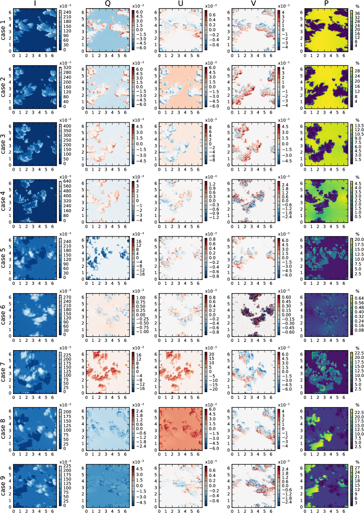
Figure 27: Results for scenario C3 (cumulus clouds surrounded by molecular atmosphere).

Figure 28: Results for scenario C3 (cumulus clouds in molecular atmosphere with aerosol).

References

- Emde et al. [2015] C. Emde, V. Barlakas, C. Cornet, F. Evans, S. Korkin, Y. Ota, L. C. Labonnote, A. Lyapustin, A. Macke, B. Mayer, M. Wendisch, IPRT polarized radiative transfer model intercomparison project - Phase A, J. Quant. Spectrosc. Radiat. Transfer 164 (0) (2015) 8–36, ISSN 0022-4073, doi:10.1016/j.jqsrt.2015.05.007, URL http://www.sciencedirect.com/science/article/pii/S0022407315001922.
- Deschamps et al. [1994] P.-Y. Deschamps, F.-M. Breon, M. Leroy, A. Podaire, A. Bricaud, J.-C. Buriez, G. Seze, The POLDER mission: instrument characteristics and scientific objectives, IEEE Transactions on Geoscience and Remote Sensing 32 (1994) 598–615, doi:10.1109/36.297978.
- Bréon and Doutriaux-Boucher [2005] F.-M. Bréon, M. Doutriaux-Boucher, A comparison of Cloud Droplet Radii Measured from Space, IEEE Transactions on Geoscience and Remote Sensing 43 (8) (2005) 1769–1805.
- Waquet et al. [2013] F. Waquet, C. Cornet, J.-L. Deuzé, O. Dubovik, F. Ducos, P. Goloub, M. Herman, T. Lapyonok, L. C. Labonnote, J. Riedi, D. Tanré, F. Thieuleux, C. Vanbauce, Retrieval of aerosol microphysical and optical properties above liquid clouds from POLDER/PARASOL polarization measurements, Atmospheric Measurement Techniques 6 (4) (2013) 991–1016, doi:10.5194/amt-6-991-2013, URL http://www.atmos-meas-tech.net/6/991/2013/.
- Dubovik et al. [2011] O. Dubovik, M. Herman, A. Holdak, T. Lapyonok, D. Tanré, J. L. Deuzé, F. Ducos, A. Sinyuk, A. Lopatin, Statistically optimized inversion algorithm for enhanced retrieval of aerosol properties from spectral multi-angle polarimetric satellite observations, Atmospheric Measurement Techniques 4 (5) (2011) 975–1018, doi:10.5194/amt-4-975-2011, URL http://www.atmos-meas-tech.net/4/975/2011/.
- Xu et al. [2017] F. Xu, G. van Harten, D. J. Diner, O. V. Kalashnikova, F. C. Seidel, C. J. Bruegge, O. Dubovik, Coupled retrieval of aerosol properties and land surface reflection using the Airborne Multiangle SpectroPolarimetric Imager (AirMSPI), J. Geophys. Res. 122 (2017) 7004–7026.
- Maignan et al. [2009] F. Maignan, F.-M. Bréon, E. Fédèle, M. Bouvier, Polarized reflectances of natural surfaces: Spaceborne measurements and analytical modeling, Remote Sens. Environ. 113 (12) (2009) 2642–2650.
- Marbach et al. [2015] T. Marbach, J. Riedi, A. Lacan, P. Schlüssel, The 3MI mission: multi-viewing-channel-polarisation imager of the EUMETSAT polar system: second generation (EPS-SG) dedicated to aerosol and cloud monitoring., Proc. SPIE doi:10.1117/12.2186978.
- Liu and Diner [2017] Y. Liu, D. J. Diner, Multi-Angle Imager for Aerosols: A satellite investigation to benefit public health, Public Health Reports 132 (1) (2017) 14–17.
- Diner et al. [2012] D. J. Diner, F. Xu, J. V. Martonchik, B. E. Rheingans, S. Geier, V. M. Jovanovic, A. Davis, R. A. Chipman, S. C. McClain, Exploration of a polarized surface bidirectional reflectance model using the ground-based multiangle spectropolarimetric imager, Atmosphere 3 (2012) 591–619, doi:doi:10.3390/atmos3040591.
- van Harten et al. [2011] G. van Harten, F. Snik, J. H. H. Rietjens, J. M. Smit, J. de Boer, R. Diamantopoulou, O. P. Hasekamp, D. M. Stam, C. U. Keller, E. C. Laan, A. L. Verlaan, W. A. Vliegenthart, R. ter Horst, R. Navarro, K. Wielinga, S. Hannemann, S. G. Moon, R. Voors, Prototyping for the Spectropolarimeter for Planetary EXploration (SPEX): calibration and sky measurements, Proc.SPIE 8160 (2011) 8160 – 8160 – 12, doi:10.1117/12.893741, URL http://dx.doi.org/10.1117/12.893741.
- Cairns et al. [1999] B. Cairns, E. E. Russell, L. D. Travis, Research Scanning Polarimeter: calibration and ground-based measurements, in: Proceedings of SPIE - The International Society for Optical Engineering, vol. 3754, 186–196, 1999.
- Cairns et al. [2003] B. Cairns, E. Russell, J. LaVeigne, P. Tennant, Research scanning polarimeter and airborne usage for remote sensing of aerosols, in: Proceedings of SPIE - The International Society for Optical Engineering, vol. 5158, 33–44, 2003.
- Davis et al. [2013] A. B. Davis, M. J. Garay, F. Xu, Z. Qu, C. Emde, 3D radiative transfer effects in multi-angle/multispectral radio-polarimetric signals from a mixture of clouds and aerosols viewed by a non-imaging sensor, Proc. SPIE 8873 (2013) 887309–887309–18, doi:10.1117/12.2023733.
- Mishchenko et al. [2007] M. I. Mishchenko, B. Cairns, G. Kopp, C. F. Schueler, B. A. Fafaul, J. E. Hansen, R. J. Hooker, T. Itchkawich, H. B. Maring, L. D. Travis, Accurate Monitoring of Terrestrial Aerosols and Total Solar Irradiance: Introducing the Glory Mission, Bulletin of the American Meteorological Society 88, doi:10.1175/BAMS-88-5-677.
- Stap et al. [2016a] F. Stap, O. Hasekamp, C. Emde, T. Röckmann, Influence of 3D effects on 1D aerosol retrievals in synthetic, partially clouded scenes, J. Quant. Spectrosc. Radiat. Transfer 170 (2016a) 54 – 68, ISSN 0022-4073, doi:http://dx.doi.org/10.1016/j.jqsrt.2015.10.008, URL http://www.sciencedirect.com/science/article/pii/S0022407315300443.
- Stap et al. [2016b] F. A. Stap, O. P. Hasekamp, C. Emde, T. Rockmann, Multiangle photopolarimetric aerosol retrievals in the vicinity of clouds: Synthetic study based on a large eddy simulation, J. Geophys. Res. 121 (21) (2016b) 12914–12935, ISSN 2169-897X, doi:–10.1002/2016JD024787˝.
- Cornet et al. [2017] C. Cornet, L. C-Labonnote, F. Szczap, L. Deaconu, F. Waquet, F. Parol, Vanbauce, F. Thieuleux, J. Riedi, Assessments of Cloud Heterogeneity on the Multi-angular Total and Polarized Reflectances from POLDER3/PARASOL: Effects on cloud parameters and aerosol above cloud retrievals, AMT Submitted.
- Wen et al. [2013] G. Wen, A. Marshak, R. C. Levy, L. A. Remer, N. G. Loeb, T. Varnai, R. F. Cahalan, Improvement of MODIS aerosol retrievals near clouds, J. Geophys. Res. 118 (16) (2013) 9168–9181, ISSN 2169-897X, doi:–10.1002/jgrd.50617˝.
- Várnai et al. [2013] T. Várnai, A. Marshak, W. Yang, Multi-satellite aerosol observations in the vicinity of clouds, Atmos. Chem. Phys. 13 (8) (2013) 3899–3908, doi:10.5194/acp-13-3899-2013, URL https://www.atmos-chem-phys.net/13/3899/2013/.
- Martin et al. [2014] W. Martin, B. Cairns, G. Bal, Adjoint methods for adjusting three-dimensional atmosphere and surface properties to fit multi-angle/multi-pixel polarimetric measurements, J. Quant. Spectrosc. Radiat. Transfer 144 (2014) 68–85, ISSN 0022-4073, doi:–10.1016/j.jqsrt.2014.03.030˝.
- Martin and Hasekamp [2018] W. G. Martin, O. P. Hasekamp, A demonstration of adjoint methods for multi-dimensional remote sensing of the atmosphere and surface, J. Quant. Spectrosc. Radiat. Transfer 204 (Supplement C) (2018) 215 – 231, ISSN 0022-4073, doi:https://doi.org/10.1016/j.jqsrt.2017.09.031, URL http://www.sciencedirect.com/science/article/pii/S0022407317305198.
- Evans [1998] K. F. Evans, The spherical harmonics discrete ordinate method for three–dimensional atmospheric radiative transfer, J. Atmos. Sci. 55 (1998) 429–446.
- Levis et al. [2015] A. Levis, Y. Y. Schechner, A. Aides, A. B. Davis, Airborne Three-Dimensional Cloud Tomography, in: The IEEE International Conference on Computer Vision (ICCV), 2015.
- Levis et al. [2017] A. Levis, Y. Y. Schechner, A. B. Davis, Multiple-Scattering Microphysics Tomography, in: the 30th IEEE/CVF Conference on Computer Vision and Pattern Recognition (CVPR17), 2017.
- Alexandrov et al. [2012] M. D. Alexandrov, B. Cairns, C. Emde, A. S. Ackerman, B. van Diedenhoven, Accuracy assessments of cloud droplet size retrievals from polarized reflectance measurements by the research scanning polarimeter, Remote Sensing of Environment 125 (0) (2012) 92 – 111.
- Barlakas et al. [2016] V. Barlakas, A. Macke, M. Wendisch, SPARTA – Solver for Polarized Atmospheric Radiative Transfer Applications: Introduction and application to Saharan dust fields, J. Quant. Spectrosc. Radiat. Transfer 178 (2016) 77 – 92, URL doi:10.1016/j.jqsrt.2016.02.019.
- Barlakas [2016] V. Barlakas, A New Three–Dimensional Vector Radiative Transfer Model and Applications to Saharan Dust Fields, Ph.D. thesis, University of Leipzig, Faculty of Physics and Earth Sciences, URL http://www.qucosa.de/recherche/frontdoor/?tx_slubopus4frontend[id]=20746, 2016.
- Kotchenova et al. [2006] S. Y. Kotchenova, E. F. Vermote, R. Matarrese, J. Frank J. Klemm, Validation of a vector version of the 6S radiative transfer code for atmospheric correction of satellite data. Part I: Path radiance, Appl. Opt. 45 (2006) 6762–6774.
- Cahalan et al. [2005] R. Cahalan, L. Oreopoulos, A. Marshak, K. Evans, A. Davis, R. Pincus, K. Yetzer, B. Mayer, R. Davies, T. Ackerman, B. H.W., E. Clothiaux, R. Ellingson, M. Garay, E. Kassianov, S. Kinne, A. Macke, W. O’Hirok, P. Partain, S. Prigarin, A. Rublev, G. Stephens, F. Szczap, E. Takara, T. Varnai, G. Wen, T. Zhuraleva, The International Intercomparison of 3D Radiation Codes (I3RC): Bringing together the most advanced radiative transfer tools for cloudy atmospheres, Bulletin of the American Meteorological Society 86 (9) (2005) 1275–1293.
- Loughman et al. [2004] R. P. Loughman, E. Griffioen, L. Oikarinen, O. V. Postylyakov, A. Rozanov, D. E. Flittner, D. F. Rault, Comparison of radiative transfer models for limb-viewing scattered sunlight measurements, J. Geophys. Res. 109 (6).
- Melsheimer et al. [2005] C. Melsheimer, C. Verdes, S. A. Buehler, C. Emde, P. Eriksson, D. G. Feist, S. Ichizawa, V. O. John, Y. Kasai, G. Kopp, N. Koulev, T. Kuhn, O. Lemke, S. Ochiai, F. Schreier, T. R. Sreerekha, M. Suzuki, C. Takahashi, S. Tsujimaru, J. Urban, Intercomparison of general purpose clear sky atmospheric radiative transfer models for the millimeter/submillimeter spectral range, Radio Science 40 (1).
- Kokhanovsky et al. [2010] A. A. Kokhanovsky, V. P. Budak, C. Cornet, M. Duan, C. Emde, I. L. Katsev, D. A. Klyukov, S. V. Korkin, L. C-Labonnote, B. Mayer, Q. Min, T. Nakajima, Y. Ota, A. S. Prikhach, V. V. Rozanov, T. Yokota, E. P. Zege, Benchmark results in vector atmospheric radiative transfer, J. Quant. Spectrosc. Radiat. Transfer 111 (12-13) (2010) 1931–1946.
- Cornet et al. [2010] C. Cornet, L. C-Labonnote, F. Szczap, Three-dimensional polarized Monte Carlo atmospheric radiative transfer model (3DMCPOL): 3D effects on polarized visible reflectances of a cirrus cloud, J. Quant. Spectrosc. Radiat. Transfer 111 (1) (2010) 174 – 186, ISSN 0022-4073, doi:http://dx.doi.org/10.1016/j.jqsrt.2009.06.013.
- Fauchez et al. [2014] T. Fauchez, C. Cornet, F. Szczap, P. Dubuisson, T. Rosambert, Impact of cirrus clouds heterogeneities on top-of-atmosphere thermal infrared radiation, Atmos. Chem. Phys. 14 (11) (2014) 5599–5615, doi:10.5194/acp-14-5599-2014, URL http://www.atmos-chem-phys.net/14/5599/2014/.
- Wang et al. [2017] Z. Wang, S. Cui, J. Yang, H. Gao, C. Liu, Z. Zhang, A novel hybrid scattering order-dependent variance reduction method for Monte Carlo simulations of radiative transfer in cloudy atmosphere, J. Quant. Spectrosc. Radiat. Transfer 189 (2017) 283–302, doi:–10.1016/j.jqsrt.2016.12.002˝.
- Mayer [2009] B. Mayer, Radiative transfer in the cloudy atmosphere, European Physical Journal Conferences 1 (2009) 75–99.
- Emde et al. [2010] C. Emde, R. Buras, B. Mayer, M. Blumthaler, The impact of aerosols on polarized sky radiance: model development, validation, and applications, Atmos. Chem. Phys. 10 (2) (2010) 383–396.
- Emde et al. [2016] C. Emde, R. Buras-Schnell, A. Kylling, B. Mayer, J. Gasteiger, U. Hamann, J. Kylling, B. Richter, C. Pause, T. Dowling, L. Bugliaro, The libRadtran software package for radiative transfer calculations (version 2.0.1), Geophy. Mod. Dev. 9 (5) (2016) 1647–1672, doi:10.5194/gmd-9-1647-2016, URL http://www.geosci-model-dev.net/9/1647/2016/.
- Wang et al. [2011] Z. Wang, S. Yang, Y. Qiao, S. Cui, Q. Zhao, Multiple-scaling methods for Monte Carlo simulations of radiative transfer in cloudy atmosphere, J. Quant. Spectrosc. Radiat. Transfer 2619–2629.
- Wang et al. [2012] Z. Wang, S. Yang, Y. Qiao, S. Cui, Q. Zhao, Monte Carlo Simulations of Radiative Transfer in Cloudy Atmosphere over Sea Surfaces, Terr. Atmos. Ocean. Sci. 23 (1) (2012) 59–70, ISSN 1017-0839, doi:–10.3319/TAO.2011.08.29.01(A)˝.
- Chandrasekhar [1950] S. Chandrasekhar, Radiative transfer, Oxford Univ. Press, UK, 1950.
- Hansen and Travis [1974] J. E. Hansen, L. D. Travis, Light scattering in planetary atmospheres, Space Science Reviews 16 (1974) 527–610.
- Mishchenko et al. [2002] M. I. Mishchenko, L. Travis, A. Lacis, Scattering, Absorption, and Emission of Light by Small Particles, Cambridge University Press, 2002.
- Wendisch and Yang [2012] M. Wendisch, P. Yang, Theory of Atmospheric Radiative Transfer, A Comprehensive Introduction, Wiley-VCH Verlag GmbH & Co. KGaA, Weinheim, Germany, 2012.
- Hovenier et al. [2004] J. Hovenier, C. van der Mee, H. Domke, Transfer of polarized light in planetary atmospheres. Basic concepts and practical methods, Kluwer Academic Publishers, 2004.
- Segelstein [1981] D. J. Segelstein, The complex refractive index of water, Master’s thesis, Columbia University, 1981.
- Mishchenko [2014] M. I. Mishchenko, Directional radiometry and radiative transfer: The convoluted path from centuries-old phenomenology to physical optics, J. Quant. Spectrosc. Radiat. Transfer 146 (SI) (2014) 4–33, ISSN 0022-4073, doi:–10.1016/j.jqsrt.2014.02.033˝.
- García Muñoz [2015] A. García Muñoz, Towards a comprehensive model of Earth’s disk-integrated Stokes vector, International Journal of Astrobiology 14 (2015) 379–390, doi:10.1017/S1473550414000573.
- Buras and Mayer [2011] R. Buras, B. Mayer, Efficient unbiased variance reduction techniques for Monte Carlo simulations of radiative transfer in cloudy atmospheres: The solution, J. Quant. Spectrosc. Radiat. Transfer 112 (3) (2011) 434–447.
- Iwabuchi and Suzuki [2009] H. Iwabuchi, T. Suzuki, Fast and accurate radiance calculations using truncation approximation for anisotropic scattering phase functions, J. Quant. Spectrosc. Radiat. Transfer 110 (17) (2009) 1926–1939, ISSN 0022-4073, doi:–10.1016/j.jqsrt.2009.04.006˝.
- García Muñoz and Mills [2015] A. García Muñoz, F. P. Mills, Pre-conditioned backward Monte Carlo solutions to radiative transport in planetary atmospheres. Fundamentals: Sampling of propagation directions in polarising media, Astron. Astrophys. 573 A72, doi:10.1051/0004-6361/201424042.
- Stevens et al. [1999] B. Stevens, C. H. Moeng, P. P. Sullivan, Large-eddy simulations-of radiatively driven convection: Sensitivities to the representation of small scales, J. Atmos. Sci. 56 (1999) 3963–3984.
- Hess et al. [1998] M. Hess, P. Koepke, I. Schult, Optical Properties of Aerosols and Clouds: The Software Package OPAC, Bulletin of the American Meteorological Society 79 (5) (1998) 831–844.