IPRT polarized radiative transfer model intercomparison project – phase A

Abstract

The polarization state of electromagnetic radiation scattered by atmospheric particles such as aerosols, cloud droplets, or ice crystals contains much more information about the optical and microphysical properties than the total intensity alone. For this reason an increasing number of polarimetric observations are performed from space, from the ground and from aircraft. Polarized radiative transfer models are required to interpret and analyze these measurements and to develop retrieval algorithms exploiting polarimetric observations. In the last years a large number of new codes have been developed, mostly for specific applications. Benchmark results are available for specific cases, but not for more sophisticated scenarios including polarized surface reflection and multi-layer atmospheres. The International Polarized Radiative Transfer (IPRT) working group of the International Radiation Commission (IRC) has initiated a model intercomparison project in order to fill this gap. This paper presents the results of the first phase A of the IPRT project which includes ten test cases, from simple setups with only one layer and Rayleigh scattering to rather sophisticated setups with a cloud embedded in a standard atmosphere above an ocean surface. All scenarios in the first phase A of the intercomparison project are for a one-dimensional plane-parallel model geometry. The commonly established benchmark results are available at the IPRT website (http://www.meteo.physik.uni-muenchen.de/~iprt).

1 Introduction

An increasing number of remote sensing instruments measure the polarization state of electromagnetic radiation. Therefore, polarized radiative transfer codes are required to interpret and analyze the measurements and to develop retrieval algorithms. Sensors that measure polarization from space are, e.g., the Polarization and Directionality of the Earth׳s Reflectances (POLDER) instrument onboard PARASOL (Polarization and Anisotropy of Reflectances for Atmospheric Sciences coupled with Observations from a Lidar) [Deschamps et al., 1994] and the Thermal and Near Infrared Sensor for Carbon Observation Fourier-Transform Spectrometer (TANSO-FTS) on the Greenhouse gas Observing SATellite GOSAT [Kuze et al., 2009]. Future missions include e.g. the Climate Absolute Radiance and Refractivity Observatory (CLARREO) [Wielicki et al., 2013] and the Multi-Viewing Multi-Channel Multi-Polarization Imaging mission (3MI) on METOP-SG (Meteorological Operational Satellite - Second Generation). All-sky imaging systems are available to measure the polarized radiance distribution; such systems are described for instance by Liu and Voss [1997], Kreuter et al. [2009] and references therein. The Research Scanning Polarimeter (RSP) [Cairns et al., 1999, 2003] has been used for ground-based as well as airborne aerosol measurements. Other multi-channel polarimetric instruments are the Airborne Multiangle SpectroPolarimetric Imager (AirMSPI) [Diner et al., 2012] and the Observing System Including PolaRisation in the Solar Infrared Spectrum (OSIRIS) [aur, 2008]. The commercially available ground-based polarimeter, CE318-DP, developed by CIMEL Electronic (Paris, France) is now available at several AERONET stations [Li et al., 2014].

A large number of models for polarized radiative transfer have been developed in the last years for various specific applications. They mostly have been validated against existing benchmark data; e.g., Coulson et al. [1960] and Nataraj et al. [2009] for Rayleigh scattering; e.g., de Haan et al. [1987], Wauben et al. [1994], Garcia and Siewert [1989] for layers including aerosols; and Kokhanovsky et al. [2010] for cloud and aerosol scattering including realistic phase matrices. More references to published benchmark results are given on the IPRT website, section “benchmark results”. However, all existing benchmark results are limited to one or two plane-parallel layers with an underlying Lambertian surface. To simulate the measurements of the above mentioned sensors, far more realistic settings are required. Reasonable height profiles of molecules, aerosols and clouds should be taken into account. For clear-sky atmospheres, a plane-parallel model geometry is a reasonable approximation. When clouds are analyzed it is also important to look into effects resulting from the geometrical structure of clouds, commonly called 3D-effects, hence validated 3D vector radiative transfer codes are required. In order to simulate limb observations, fully spherical vector codes are needed. Polarization by the surface must be considered, in particular for aerosol remote sensing from space.

In order to support model developers and to set standards for polarized radiative transfer modeling the International Radiation Commission (IRC) has established the working group “International Polarized Radiative Transfer” (IPRT) which is charged by the task to provide benchmark data for polarized radiative transfer simulations for realistic atmospheric setups as needed to simulate the current and future satellite, airborne and ground-based polarimetric sensors. In order to establish this benchmark dataset a model intercomparison project has been launched. This paper summarizes the results from the first phase of the project. Six vector radiative transfer models from various international institutions have participated. The models use different approaches to solve the vector radiative transfer equation, among them are deterministic approaches based on discrete ordinates or spherical harmonics and also statistical approaches based on Monte Carlo methods. The test cases in the first phase include simple one-layer setups, cases with polarized surface reflection, and cases with realistic height profiles of molecules and aerosol particles.

The focus of this intercomparison project is the establishment of benchmark results, therefore all models were run in high accuracy mode. For realistic applications with limited computational time the models are usually run with lower accuracy. The first intercomparisons between models showed several larger differences, some of them due to model errors which have been fixed in the course of this project. The participants were allowed to provide corrected or more accurate data. Finally a very good agreement for all test cases has been found for most models. The commonly established benchmark results are available at the IPRT website (http://www.meteo.physik.uni-muenchen.de/~iprt). The next phase of the intercomparison project will start soon with focus on 3D radiative transfer.

2 Radiative transfer models

Table 1: Overview of radiative transfer models

model name	method	geometry	arbitrary output altitude	references
3DMCPOL	Monte Carlo	1D/3D	no	Cornet et al. [2010], Fauchez et al. [2014]
IPOL	discrete ordinate	1D	no	ftp://climate1.gsfc.nasa.gov/skorkin/IPOL/
MYSTIC	Monte Carlo	1D/3D(a)	yes	Mayer [2009], Emde et al. [2010]
Pstar	discrete ordinate	1D	yes	Ota et al. [2010]
SHDOM	spherical harmonics discrete ordinate	1D/3D	yes	Evans [1998]
SPARTA	Monte Carlo	1D/3D	no	Barlakas et al. [2014]
(a)MYSTIC includes fully spherical geometry for 1D and 3D.

2.1 3DMCPOL

3DMCPOL is a forward Monte-Carlo model for radiative transfer in three-dimensional atmosphere. It can compute the reflected or transmitted Stokes vector as well as upwelling and downwelling fluxes. Initially developed for solar radiation [Cornet et al., 2010], it was recently extended to thermal radiation [Fauchez et al., 2014]. To save time and for an accurate computation of radiances, it uses the Local Estimate Method [Marshak and Davis, 2005, Mayer, 2009]. The medium is divided into voxels (3D pixels) with constant cloud and aerosol optical properties, that are the extinction coefficient, the single scattering albedo, the phase function and the cloud temperature. For highly peaked phase functions, the truncation of Potter [1970] is implemented and we also added recently the variance reduction method of Buras and Mayer [2011]. Atmospheric profiles including temperature, pressure and absorption coefficient of a correlated k-distribution can also be specified. The molecular scattering is computed automatically according to the pressure profile. A depolarization factor can be specified. To save substantial time, the absorption computation is done following the Equivalence Theorem [Partain et al., 2000, Emde et al., 2011]: the computation of radiative transfer trough the scattering medium is done once and the radiances are attenuated according to the absorption coefficient of the k-distribution along the geometrical path of the photons. A heterogeneous surface can also be specified with Lambertian reflection, ocean or snow bidirectional function. 3DMCPOL applications concern mainly the cloud heterogeneities effects on total and polarized radiances and the errors on retrieved parameters from passive sensors. For example, for the polarized and multi-angular radiometer POLDER3/PARASOL, 3DMCPOL was used to study on synthetic data the bias for retrieved optical thickness and effective radius [Cornet et al., 2013] and also to test aerosol above cloud retrieval [Waquet et al., 2013]. Studies on the thermal radiation were also conducted to assess the bias due to cirrus heterogeneity on the brightness temperature measured by the radiometer IIR/CALIPSO [Fauchez et al., 2014] and on the retrieved effective optical thickness and effective diameters [Fauchez et al., 2015]. For this intercomparison project 10⁸ photons were used for simulations without ocean and 10⁷ photons for simulations including an ocean surface. For ocean reflection, the polarized bidirectional reflectance contribution function and corresponding probability densities are computed at the beginning of the simulation and during the calculation interpolations are done to obtain the new direction and the contribution to the top of the atmosphere. These interpolations increase computational time, therefore less photons were used for the simulations with ocean.

2.2 IPOL

IPOL is a radiative transfer code that computes Intensity and POLarization of radiation reflected from or transmitted through the Earth atmosphere over a reflecting surface. Radiation field inside the atmosphere is not computed thus saving computation time and memory. The code is suitable for remote sensing systems located on the ground and aboard satellites or high altitude aircrafts. The code is written in Fortran 90/95, requires external BLAS-LAPACK libraries, and is freely available for downloading from ftp://climate1.gsfc.nasa.gov/skorkin/IPOL/.

Following libRadtran and XRTM (http://reef.atmos.colostate.edu/~gregm/xrtm/), IPOL will soon incorporate several solvers for the vector radiative transfer equation. This allows for fast yet accurate computation in a variety of scenarios. In this intercomparision, only the discrete ordinates solver is validated. The next solver to be included in the IPOL project, SORD (Successive ORDers of scattering), currently undergoes intensive testing. SORD is already available at ftp://climate1.gsfc.nasa.gov/skorkin/SORD/.

In IPOL, the system of coordinates and direction of positive rotation of the frame of reference is defined exactly following Hovenier et al. [2004, p. 11 and Sec. 3.2]. The Stokes vector is computed at arbitrary viewing directions, except for the horizon, using the dummy-node technique [Chalhoub and Garcia, 2000]. Singular value decomposition is used to solve the system of equations at Gauss and dummy nodes. Scaling transformation [Karp et al., 1980] stabilizes the solution of the system for an arbitrary atmospheric optical thickness. Layers with different optical properties and a reflecting surface are bound together using the matrix-operator method [Nakajima and Tanaka, 1986, Plass et al., 1973, Ota et al., 2010]. Single scattering path radiance and reflection of the direct solar beam from the surface are computed analytically. In order to avoid errors in the aureole [Korkin et al., 2012], none of the phase function truncation techniques [Rozanov and Lyapustin, 2010] has been implemented so far. IPOL ignores atmospheric curvature, 3D effects, and thermal emission. We have tested IPOL against the vector codes APC [Korkin et al., 2013], RT3 [Evans and Stephens, 1991], SCIATRAN [Rozanov et al., 2013], and the published results (see references in the Introduction). The radiative transfer code SHARM [Lyapustin, 2005] was used to test the total intensity. Scalar surface models and interface for IPOL were adapted from SHARM as well.

IPOL was run with 16 streams (half-sphere) for all Rayleigh and the spherical aerosol case, with 128 streams for the spheroidal aerosol cases, and with 256 streams for all cloud cases to ensure high accuracy of benchmark results.

2.3 MYSTIC

The radiative transfer model MYSTIC (Monte-Carlo code for the phYsically correct Tracing of photons in Cloudy atmospheres) [Mayer, 2009] is a versatile Monte-Carlo code for atmospheric radiative transfer which is operated as one of several radiative transfer solvers of the libRadtran software package [Mayer and Kylling, 2005]. The 1D version of MYSTIC is freely available at http://www.libradtran.org. MYSTIC may be used to calculate polarized solar and thermal radiances, and also for irradiances, actinic fluxes and heating rates [Klinger and Mayer, 2014]. The model has been used extensively to generate realistic synthetic measurements for the validation of various retrieval algorithms for cloud and aerosol properties [Davis et al., 2013, Bugliaro et al., 2011]. Further application fields are e.g. photochemistry [Sumińska-Ebersoldt et al., 2012] or remote sensing of exo-planets. MYSTIC allows the definition of arbitrarily complex 3D clouds and aerosols, an inhomogeneous surface albedo and topography. Polarized surface reflection is also included. The model can be operated in fully spherical geometry [Emde and Mayer, 2007], hence it can also be used for limb sounding applications. Polarization has been included by combining various methods [Emde et al., 2010]. The local estimate method [Marchuk et al., 1980, Marshak and Davis, 2005] has been adapted to account for polarization, which is essential for accurate radiance simulations. An importance sampling method similar to Collins et al. [1972] is used to sample the photon direction after scattering or surface reflection, the probability of which depends not only on the scattering angle (as in scalar radiative transfer) but also on the relative azimuth angle between incident and scattered direction. Sophisticated variance reduction methods are included [Buras and Mayer, 2011] which allow to calculate unbiased radiances for scattering media characterized by strongly peaked phase functions without any approximations. It is also possible to calculate polarized radiances in high spectral resolution efficiently [Emde et al., 2011]. For all cloudless simulations shown in this intercomparison $10^{8}$ photons were run and for the simulations including clouds $10^{7}$ photons were used. For clouds less photons were used because of the much larger computational time due to multiple scattering. Even though only $10^{7}$ photons were used, the results are not too noisy because of the sophisticated variance reduction methods included in MYSTIC.

2.4 Pstar

The radiative transfer (RT) code, Pstar, has been developed to simulate the polarized radiation field of a vertically inhomogeneous 1D system as approximated by several homogeneous layers [Ota et al., 2010]. Pstar has been used to simulate polarized solar and thermal radiation as measured by satellite, and to develop an aerosol retrieval algorithm, an atmospheric correction algorithm, and a vicarious calibration system that include the polarization effect (e.g. Fukuda et al. [2013], Murakami and Dupouy [2013]). The RT scheme of Pstar is constructed using the discrete ordinate method and the matrix operator method. The discrete ordinate method is applied to each homogeneous layer in order to obtain the reflection/transmission matrices and the source vector of the layer. Then, the matrix operator method is applied to all layers to obtain the radiation field of the multi-layered system. The Stokes parameters at any interfaces between the homogeneous layers as well as at the top of the atmosphere and at any propagation direction are obtained by post-processing using the source function integration technique. Finally, more accurate Stokes parameters are obtained using the single scattering correction procedure. This RT scheme is originally based on the formulations of Nakajima and Tanaka [1986, 1988], which are implemented as the scalar RT code series of System for Transfer of Atmospheric Radiation (STAR) [Ruggaber et al., 1994]. Ota et al. [2010] have extended the RT formulation to express the polarized radiation field and implemented it in Pstar code. The extended RT scheme is constructed to be flexible for a vertically inhomogeneous system including the oceanic layers as well as the ocean surface. Accordingly, Pstar can be used to simulate the radiation field in the coupled atmosphere-ocean system including the polarization effect. Pstar computes all four Stokes parameters in the vector mode, although only the total radiance (I) is obtained in the scalar mode. Furthermore, the semi-vector mode that computes the three Stokes parameters (I, Q, and U) on the basis of the 3x3 phase matrix approximation is available. The computation of eigen solutions of the discrete ordinate method is one of the most time consuming parts. In the vector mode, the direct decomposition method [Ota et al., 2010] is used in order to acquire the complex eigen solutions, which is necessary to calculate the Stokes parameter V accurately. However, in the scalar and semi-vector modes, a square-root decomposition technique as described by Nakajima and Tanaka [1986] is invoked to obtain the real eigen solutions efficiently. In the inter-comparison of this paper, the vector mode was used to compute four Stokes parameters. In the Rayleigh scattering cases, 15 streams were used for both single and multi-layer conditions. In the aerosol and cloud scattering cases, 90 streams were used for single-layer cases and 30 streams for multi-layer cases. The number of streams refer to the half-sphere.

2.5 SHDOM

The spherical harmonics discrete ordinate method (SHDOM) was developed for unpolarized 3D atmospheric radiative transfer [Evans, 1998]. SHDOM is a non-Monte Carlo method in that the radiation field in the domain is discretized and solved for iteratively. The source function is discretized with a spherical harmonics series for the angular aspect and grid points in a cartesian geometry for the spatial aspect. For computational efficiency an adaptive grid is used in which addition grid points may be added to the regular base grid where the source function is changing rapidly, such as at illuminated cloud boundaries. The solution iterations consist of 1) transforming the source function from spherical harmonics to discrete ordinates, 2) integrating the source function along discrete ordinates to obtain the radiance field, 3) transforming the radiance field to spherical harmonics, and 4) computing the source function (including the scattering integral) efficiently in spherical harmonics from the radiance. A sequence acceleration method is used to speed up convergence of the iterations. For highly-peaked phase functions the delta-M method is used and the output radiance is computed with the TMS method of Nakajima and Tanaka [1988], in which the single scattering contribution is calculated with the exact phase function instead of the truncated spherical harmonics approximation. SHDOM does not implement higher order scattering corrections and thus does not provide accurate results for highly-peaked (i.e. cloud) phase functions in the solar aureole region.

The SHDOM model can calculate the radiance field from solar and/or thermal emission sources of radiation. The extinction and single scattering albedo of the medium are specified on a 3D grid and trilinearly interpolated between grid points. Instead of specifying the phase matrix at every grid point, to save memory, a table of expansion coefficients for many phase matrices is input, and each grid point has a specified index into the phase matrix table. Once the SHDOM iterations are completed, radiances in many directions on a grid at any height, hemispheric fluxes, net fluxes, mean radiances, and net flux convergence may be efficiently computed. Several types of bidirectional reflection distribution function (BRDF) models for the surface are implemented, and their parameters may vary across the domain. A k-distribution approach is used to integrate across spectral bands. For large 3D domains SHDOM may be run on multiple processors using the Message Passing Interface [Pincus and Evans, 2009]. SHDOM is distributed from http://coloradolinux.com/shdom/.

Recently polarization capability was added to SHDOM using the real generalized spherical harmonics method of Doicu et al. [2013]. Key pieces of Adrian Doicu’s VSHDOM research code were adapted for use in polarized SHDOM. The generalized spherical harmonics basis uses 4x4 matrices, $\mathsf{Y}_{lm}(\mu,\phi)$ with 6 non-zero elements (including a 2x2 block for $Q$ and $U$). The angles $\mu=\cos(\theta)$ and $\phi$ describe the radiance direction, where $\theta$ is the zenith angle and $\phi$ is the azimuth angle in polar coordinates. The elements of the $\mathsf{Y}_{lm}$ matrix are various Wigner d-functions in $\mu$ multiplied by Fourier functions in $\phi$. The radiance and source function are represented by vectors with $N_{stokes}=1$ (scalar), 3, or 4 elements, and thus the memory use for a polarized calculation is about $N_{stokes}$ times that for a scalar calculation. SHDOM has special purpose subroutines for the unpolarized case ($N_{stokes}=1$) so the polarized code serves efficiently for scalar calculations. There are two polarized surface reflection models: Fresnel surface with waves [Mishchenko and Travis, 1997] used for ocean, and depolarizing modified-RPV (including the hotspot) with polarizing Fresnel reflection from randomly oriented microfacets [Diner et al., 2012] used for land. When enough memory is available, the surface BRDF is precomputed for all incoming and outgoing discrete ordinates, greatly speeding up computation for uniform non-Lambertian surfaces. The polarized SHDOM distribution includes Mie and T-matrix [Mishchenko and Travis, 1998] codes for generating SHDOM scattering tables from spherical or spheroidal/cylindrical shaped particles, respectively. The six unique elements of the phase matrices are represented as series expansions in Wigner d-functions (the $I-I$ and $V-V$ elements are standard Legendre polynomials).

The SHDOM results shown below are for a high resolution run with the number of discrete ordinates in zenith and azimuth angles of $N_{mu}=128$ and $N_{phi}=256$ and the cell splitting accuracy of 0.00003.

2.6 SPARTA

The Solver for Polarized Atmospheric Radiative Transfer Applications (SPARTA) is a new three-dimensional (3D) vector radiative transfer model introduced in Barlakas et al. [2014]. When finished it will become freely available. The model is based on the statistical Monte Carlo method (in the forward scheme) and calculates column-response pixel-based polarized radiances for 3D inhomogeneous cloudless and cloudy atmospheres. Hence, it is well suited for use in remote sensing applications. SPARTA is based on the established scalar Monte Carlo model of the Institute for Marine Research at the UNIversity of Kiel (MC-UNIK, Macke et al. 1999). MC-UNIK has been extended to take into account the polarization state of the electromagnetic radiation due to multiple scattering by randomly oriented non-spherical particles, i.e., coarse mode dust particles or ice particles. The SPARTA model considers a 3D Cartesian domain with a cellular structure. The latter is divided into grid-boxes, characterized by a volume extinction coefficient $\beta_{\mathrm{ext}}$ or a scattering coefficient $\beta_{\mathrm{sca}}$, a scattering phase matrix P($\Theta$) with a scattering angle $\Theta$, and a single scattering albedo $\omega_{\mathrm{o}}$. Directions are specified by the azimuth and zenith angles. Free path lengths are simulated as outlined by Marchuk et al. [1980] by random number processes with attenuation described by the law of Lambert. Scattering directions are calculated according to an importance sampling method [Collins et al., 1972, Marchuk et al., 1980, Emde et al., 2010]. Absorption is taken into account by decreasing the initial photon weight by the integrated absorption coefficient, along the photon path, according to Lambert’s law. The surface contribution is calculated assuming isotropic reflection (Lambertian surface) or ocean reflection as outlined by Mishchenko and Travis [1997]. In order to obtain precise radiance calculations for each wavelength the so-called Local Estimate Method (LEM) has been applied [Collins et al., 1972, Marchuk et al., 1980, Marshak and Davis, 2005]. Other variance reduction methods have not been implemented so far.

The selected number of photons used for all the test cases in this intercomparison was $10\textsuperscript{8}$.

3 Definition of test cases

3.1 Model coordinate system and Stokes vector

For all test cases the Stokes parameters, which are defined as time averages of linear combinations of the electromagnetic field vector [Chandrasekhar, 1950, Hansen and Travis, 1974, Mishchenko et al., 2002, Wendisch and Yang, 2012], are calculated:

$$\begin{pmatrix}I\\ Q\\ U\\ V\end{pmatrix}=\frac{1}{2}\sqrt{\frac{\epsilon}{\mu_{p}}}\begin{pmatrix}E_{l}E_{l}^{\ast}+E_{r}E_{r}^{\ast}\\ E_{l}E_{l}^{\ast}-E_{r}E_{r}^{\ast}\\ -E_{l}E_{r}^{\ast}-E_{r}E_{l}^{\ast}\\ i(E_{l}E_{r}^{\ast}-E_{r}E_{l}^{\ast})\end{pmatrix}$$ (1)

Here, $E_{l}$ and $E_{r}$ are the components of the electric field vector parallel and perpendicular to the reference plane respectively. The pre-factor on the right hand side contains the electric permittivity $\epsilon$ and the magnetic permeability $\mu_{p}$.

The model coordinate system is defined by the vertical (z-axis), the Southern direction (x-axis) and the Eastern direction (y-axis). The Stokes vector is defined in the reference frame spanned by the z-axis and the propagation direction of the radiation. The sign of Stokes parameters $U$ and $V$ depends on the definition of the model coordinate system. The results shown in this paper are for the coordinate system as defined in the books by Hovenier et al. [2004] and Mishchenko et al. [2002]. The sign of $U$ and $V$ changes when the viewing azimuthal angle definition is changed from anti-clockwise to clockwise and also when the definition of the viewing zenith angle is with respect to the downward normal instead of the upward normal. The models IPOL, SHDOM and 3DMCPOL use the definition according to Hovenier et al. [2004]. SPARTA uses a different coordinate system but the signs are consistent with Hovenier et al. [2004]. MYSTIC and Pstar also use different coordinate systems and obtain opposite signs for $U$ and $V$, all results for these Stokes components shown in this paper have been multiplied by -1.

The position of the sun is defined by the vector pointing from the surface to the sun position, i.e. the direction opposite to the propagation direction of the incoming radiation.

The degree of polarization $P$ is defined as follows:

$$P=\frac{\sqrt{(Q^{2}+U^{2}+V^{2})}}{I}$$ (2)

The definition of the test cases can also be found at http://www.meteo.physik.uni-muenchen.de/~iprt.

3.2 Test cases including a single layer

The first set of test cases are for a single layer including different atmospheric constituents, i.e. molecules, aerosols and cloud droplets. There are two cases including surface reflection, one is for a Lambertian surface and the other includes an ocean reflectance matrix.

3.2.1 A1 – Rayleigh scattering

The most simple setup contains one layer with scattering (non-absorbing) molecules. The radiation field is calculated at the top and at the bottom of the layer for various sun positions and an optical thickness of 0.5 (see Tab. 2). Viewing zenith angles range from 0^∘ to 80^∘ at the bottom and from 100^∘ to 180^∘ at the top of the layer with an increment of 5^∘. Viewing azimuth angles range from 0^∘ to 360^∘ with an increment of 5^∘. This test is partly contained in the tables by Coulson et al. [1960], Nataraj et al. [2009]. We also include non-zero solar azimuth angles to test whether the models use consistent coordinate systems to define the Stokes vector, this will be particularly important for future intercomparisons in three-dimensional geometry. Also we include a non-zero Rayleigh depolarization factor as defined in [Hansen and Travis, 1974], who defines the Rayleigh phase matrix as follows:

$${\bf P}(\Theta)=$$ (3)

$$\begin{array}[]{l}\Delta\left[\begin{array}[]{cccc}\frac{3}{4}(1+\cos^{2}\Theta)&-\frac{3}{4}\sin^{2}\Theta&0&0\\ -\frac{3}{4}\sin^{2}\Theta&\frac{3}{4}(1+\cos^{2}\Theta)&0&0\\ 0&0&\frac{3}{2}\cos\Theta&0\\ 0&0&0&\Delta^{\prime}\frac{3}{2}\cos\Theta\end{array}\right]\\[25.83325pt] \hskip 43.05542pt+(1-\Delta)\left[\begin{array}[]{cccc}\ 1&\ 0&\ 0&\ 0\\ \ 0&\ 0&\ 0&\ 0\\ \ 0&\ 0&\ 0&\ 0\\ \ 0&\ 0&\ 0&\ 0\end{array}\ \right],\end{array}$$ (14)

where

$$\Delta=\frac{1-\delta}{1+\delta/2},\qquad\Delta^{\prime}=\frac{1-2\delta}{1-\delta},$$ (15)

and $\delta$ is the depolarization factor that accounts for the anisotropy of the molecules. $\Theta$ is the scattering angle, i.e. the angle between incoming and scattered directions.

solar zenith angle $\theta_{0}$	solar azimuth angle $\phi_{0}$	depolarization factor $\delta$
0∘	65∘	0.0
30∘	0∘	0.03
30∘	65∘	0.1

Table 2: Sun positions and depolarization factors for test case A1, pure Rayleigh scattering layer.

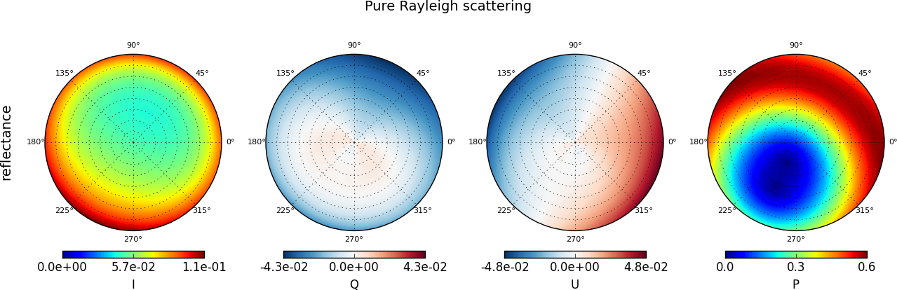
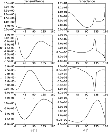
As an example Fig. 1 shows the radiation field for $\theta_{0}$=30^∘, $\phi_{0}$=65^∘, and $\delta$=0.1. The $Q$-component of the Stokes vector is negative in the principle plane. The $U$-component is zero in the principal plane and it becomes positive in the clockwise azimuthal direction and negative in the counter-clockwise direction. The maximum degree of polarization $P$ is clearly visible at a scattering angle of 90^∘.

Figure 1: Results (MYSTIC) for Rayleigh scattering layer with an optical thickness of 0.5 and a depolarization factor of 0.1. The sun position is ($\theta_{0}$=30^∘, $\phi_{0}$=65^∘).

3.2.2 A2 – Rayleigh scattering above Lambertian surface

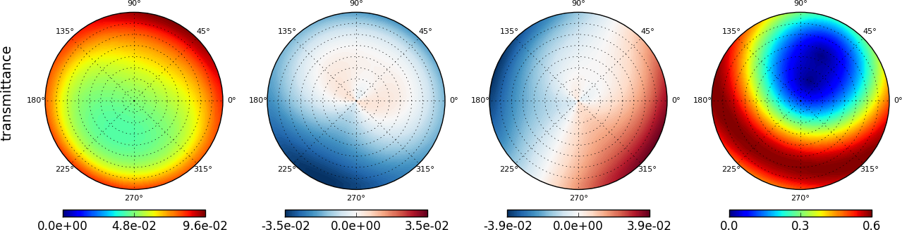
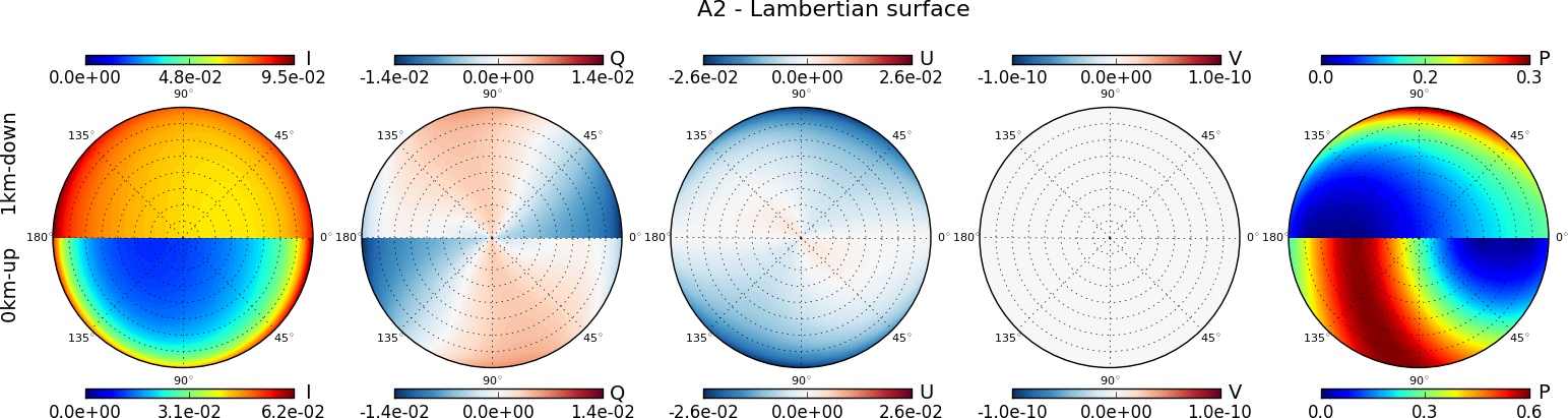
This test case includes one layer with non-absorbing molecules with an optical thickness of 0.1 above a Lambertian surface with albedo 0.3. The Rayleigh depolarization factor is 0.03 and the sun position is $(\theta_{0}=50^{\circ},\phi_{0}=0^{\circ})$. The viewing directions are as in Sec. 3.2.1. The only difference is that viewing azimuths only range from 0^∘ to 180^∘ because the radiation field is symmetric about the principal plane and the solar azimuth angle is 0^∘. The top row in Fig. 5 shows the transmittance (top part of polar plots) and the reflectance (bottom part of polar plots). The transmitted radiation field is still highly polarized whereas the degree of polarization $P$ becomes much smaller in the reflected field (from $\sim$60% in the maximum to $\sim$30%) because the total intensity becomes higher due to surface reflection. The order of magnitude of the Stokes components $Q$ and $U$ is similar in transmitted and reflected radiation fields.

3.2.3 A3 – Spherical aerosol particles

Figure 2: Phase matrices of spherical and spheroidal aerosol particles, and cloud droplets.

Here we calculate the transmitted and the reflected radiance fields for a layer including spherical aerosol particles. The optical thickness of the layer is 0.2 and the sun position is $(\theta_{0}=40^{\circ},\phi_{0}=0^{\circ})$. The aerosol microphysical properties correspond to typical water soluble aerosol for a relative humidity of 50% at 350 nm as provided in the OPAC database [Hess et al., 1998, Emde et al., 2010]: the complex refractive index is 1.422-2.649$\cdot$10^-3$i$, the size distribution is log-normal with a mode radius of 26.2 nm and a width of 2.24, and the mass density is 1.42 g/cm^-3. The optical properties including the phase matrix $P$ are calculated using the Mie tool of the libRadtran package [Mayer and Kylling, 2005, Wiscombe, 1980]. The phase matrix for randomly oriented particles depends only on the scattering angle $\Theta$:

$$\begin{array}[]{l}{\bf P}(\Theta)=\left[\begin{array}[]{cccc}P_{1}(\Theta)&P_{2}(\Theta)&0&0\\ P_{2}(\Theta)&P_{5}(\Theta)&0&0\\ 0&0&P_{3}(\Theta)&P_{4}(\Theta)\\ 0&0&-P_{4}(\Theta)&P_{6}(\Theta)\end{array}\right]\end{array}$$ (21)

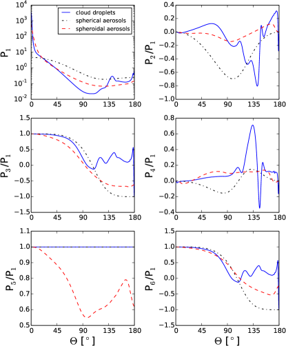
The black dashed-dotted lines in Fig. 2 show the phase matrix elements $P_{1}$–$P_{4}$. For spherical particles it has only four independent elements, $P_{5}$ is equal to $P_{1}$ and $P_{6}$ is equal to $P_{3}$. The expansion moments over generalized spherical functions (see Hovenier et al. [2004, Sec. 2.8]) for the phase matrix have also been made available for models which require those as input.

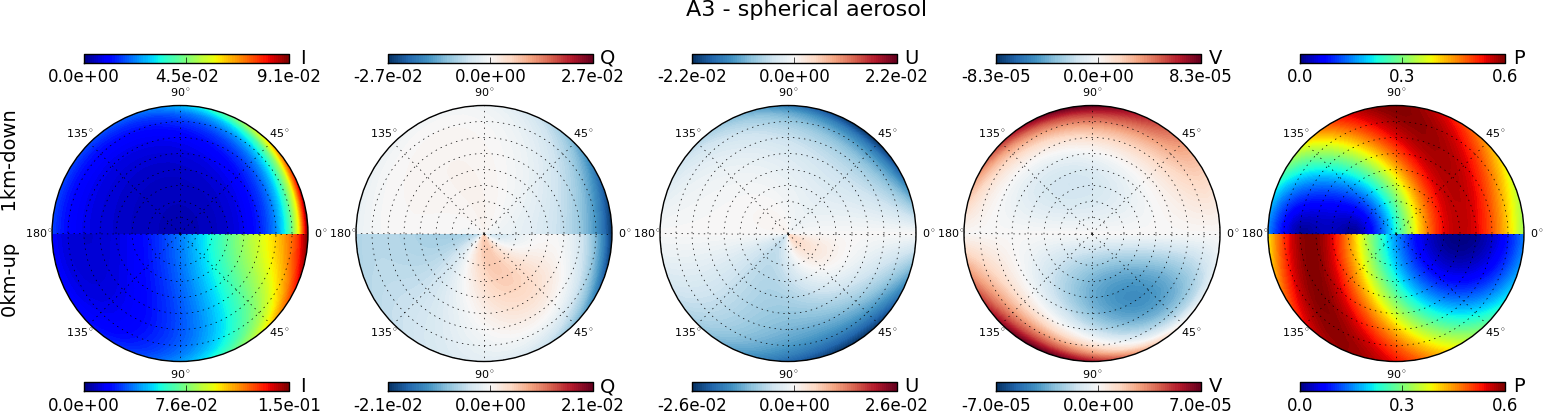
The radiance fields for this case are shown in the second row of Fig. 5. The maximum degree of polarization can be seen at a scattering angle of approximately 100^∘. The $V$-component of the Stokes vector is non-zero because scattering at spherical droplets produces circular polarization. The size parameter of this aerosol particles is small, therefore we do not see strong forward scattering in the radiance field $I$.

3.2.4 A4 – Spheroidal aerosol particles

A similar scenario as given in Sec. 3.2.3 is calculated for a layer including prolate spheroids with an aspect ratio of 3. Again a log-normal size distribution was assumed, with a mode radius of 390 nm and a width of 2. The complex refractive index is 1.52-0.01$i$ and the mass density is 2.6 g/cm^-3. The optical properties at 350 nm were calculated from a spheroid scattering data base as described by Gasteiger et al. [2011, Sec. 3.2]. The scattering data base was created using the T-matrix code by Mishchenko and Travis [1998] and the geometric optics code by Yang et al. [2007]. When the asphericity of the aerosol particles is considered the scattering phase matrix has six independent elements. The red dashed lines in Fig. 2 show the phase matrix elements for the spheroidal particles. In contrast to the spherical aerosol particles used in Sec. 3.2.3 the phase function $P_{1}$ shows much more forward scattering as the size parameter, i.e. the ratio between particle size and wavelength, is larger. Also we see a positive maximum in $P_{2}/P_{1}$ at a scattering angle of approximately 170^∘, whereas for Rayleigh scattering and for the small spherical aerosol particles this ratio is always negative. For this case the sun position is $(\theta_{0}=40^{\circ},\phi_{0}=0^{\circ})$ and the optical thickness is 0.2.

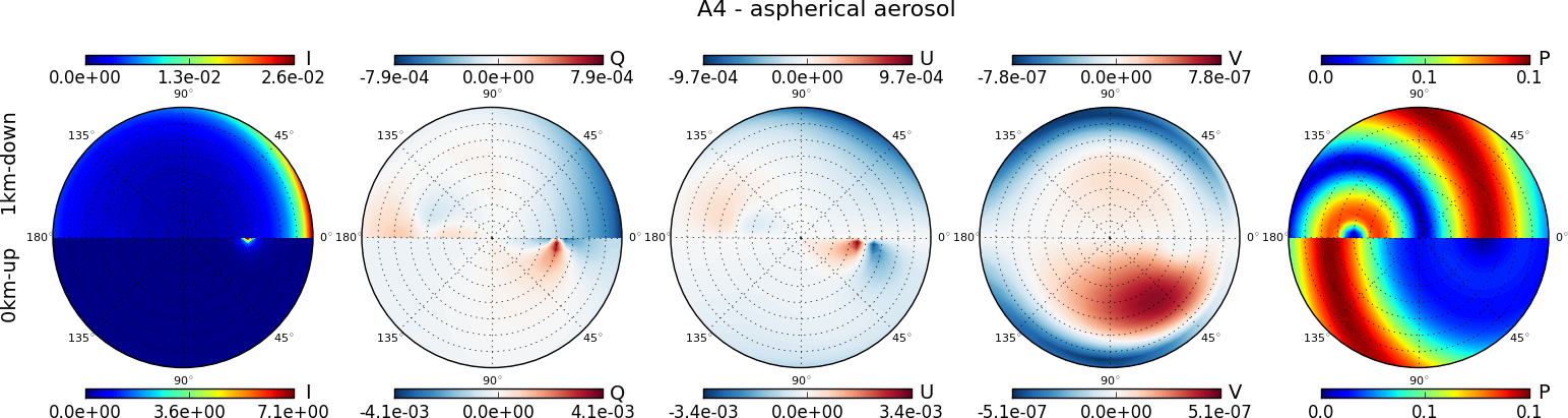
The third row in Fig. 5 shows the results for this case. The reflected radiance field (upper half of the polar plots) shows two maxima in the degree of polarization which are at the scattering angles of the minima and maxima in the ratio $P_{2}/P_{1}$. The transmitted radiance field shows high radiances $I$ in the forward scattering region. The $Q$ and $U$ components show a characteristic pattern in the forward scattering region.

3.2.5 A5 – Liquid water cloud

This test case includes a single layer with typical cloud droplets. The scattering phase matrix (see blue lines in Fig. 2) has been computed using the Mie tool of libRadtran for a wavelength of 800 nm assuming a gamma size distribution with an effective radius of 10 $\mu$m and a width of 0.1. The scattering phase matrix has the same structure as the one for spherical aerosol particles (see Eq. 21). The cloud optical thickness is set to 5. This test case is used to check whether features of the phase matrix, e.g. the cloudbow can be simulated accurately. This is particularly important because retrievals of the cloud effective radius from polarized observations use the position and the width of the cloudbow [Bréon and Doutriaux-Boucher, 2005, Alexandrov et al., 2012]. Furthermore we want to check, whether the forward scattering peak of highly asymmetric phase matrices can be taken into account accurately by the models. The sun position is at $(\theta_{0}=50^{\circ},\phi_{0}=0^{\circ})$. The radiance is calculated at an angular resolution of 1^∘ in the principal plane (i.e. $\phi\in[0^{\circ},180^{\circ}]$) at the top and at the bottom of the layer. The same angular resolution is calculated in the almucantar plane (i.e. $\theta=50^{\circ}$ and $\phi\in[0^{\circ},1^{\circ},...,180^{\circ}]$).

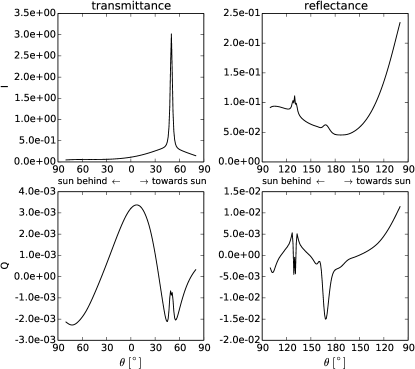
The reflected and transmitted radiances in the principal and almucantar planes are shown in Fig. 3 and Fig. 4 respectively. The $I$-component of the Stokes vector shows the strong forward scattering peak. The cloudbow can be seen in the $I$- and much more pronounced in the $Q$-component of the Stokes vector. The reason is that $Q$ is less affected by multiple scattering than $I$, because photons that are scattered multiple times have random polarization states.

Figure 3: Transmitted and reflected radiance (IPOL simulations) for a cloud layer. The viewing directions $\theta$ are in the solar principal plane ($\phi\in[0^{\circ},180^{\circ}]$).

Figure 4: Transmitted and reflected radiance (IPOL simulations) for a cloud layer. Viewing directions are in the almucantar plane ($\theta=\theta_{0},\phi\in[0^{\circ},1^{\circ},...,360^{\circ}]$).

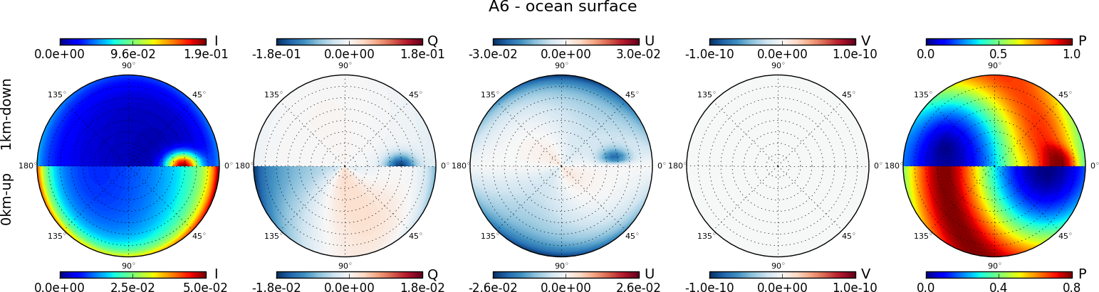
3.2.6 A6 – Rayleigh atmosphere above ocean surface

In order to test whether the surface reflection matrix is correctly included in the models, the radiance field is calculated for a Rayleigh scattering layer (optical thickness 0.1, Rayleigh depolarization factor 0.03) with an underlying ocean surface. The reflectance matrix is calculated using a combination of Fresnel equations and wave distribution including shadowing effects as implemented by Mishchenko and Travis [1997]. The real part of refractive index of water is assumed to be 1.33 and the imaginary part is zero. The wind speed is assumed to be 2 m/s. The sun position is $(\theta_{0}=45^{\circ},\phi_{0}=0^{\circ})$. The last row of Fig. 5 shows the results for this case. The sun-glint is clearly visible in the reflected radiance ( $I$, $Q$- and $U$-components of the Stokes vector). Note that the sign of $Q$ and $U$ of the reflection in the sun-glint is the same as for Rayleigh scattering.

Figure 5: Results for Lambertian surface reflection (A2, 1st row), spherical aerosol particles (A3, 2nd row), aspherical aerosol particles (A4, third row), and ocean reflectance (A6, 4th row). For details about the setup please refer to the text, Secs. 3.2.2–3.2.6. The top part of the polar plots shows the Stokes components $I$, $Q$, $U$ and $V$ and the degree of polarization $P$ of the reflected radiance field $R$ and the bottom part shows the transmitted radiance field $T$. All results shown here are calculated using MYSTIC.

3.3 Test cases with realistic atmospheric profiles

All following test cases are for the US-standard atmosphere [Anderson et al., 1986] from 0 to 30 km altitude. The atmosphere is divided into 30 layers with a thickness of 1 km. The radiance field is calculated at the surface, at the top of the atmosphere and at an altitude of 1 km. The radiance is calculated for viewing zenith angles from 0^∘ to 80^∘ (up-looking) and from 100^∘ to 180^∘ (down-looking) and for viewing azimuth angles from 0^∘ to 180^∘. The angular resolution in zenith and azimuth is 5^∘. The solar azimuth angle is generally 0^∘. The Rayleigh depolarization factor is 0.03 and the surface albedo is 0 for all cases apart from the case with ocean surface (Sec. 3.3.4).

Figure 6: Scattering , absorption and extinction coefficient profiles for multilayer test cases. The left plot shows the molecular scattering coefficient, the middle plot the molecular absorption coefficient, and the right plot the aerosol extinction coefficient. Different lines correspond to case B1 (450 nm, dash-dotted), case B2 (325 nm, solid), and case B3 (350 nm, dashed).

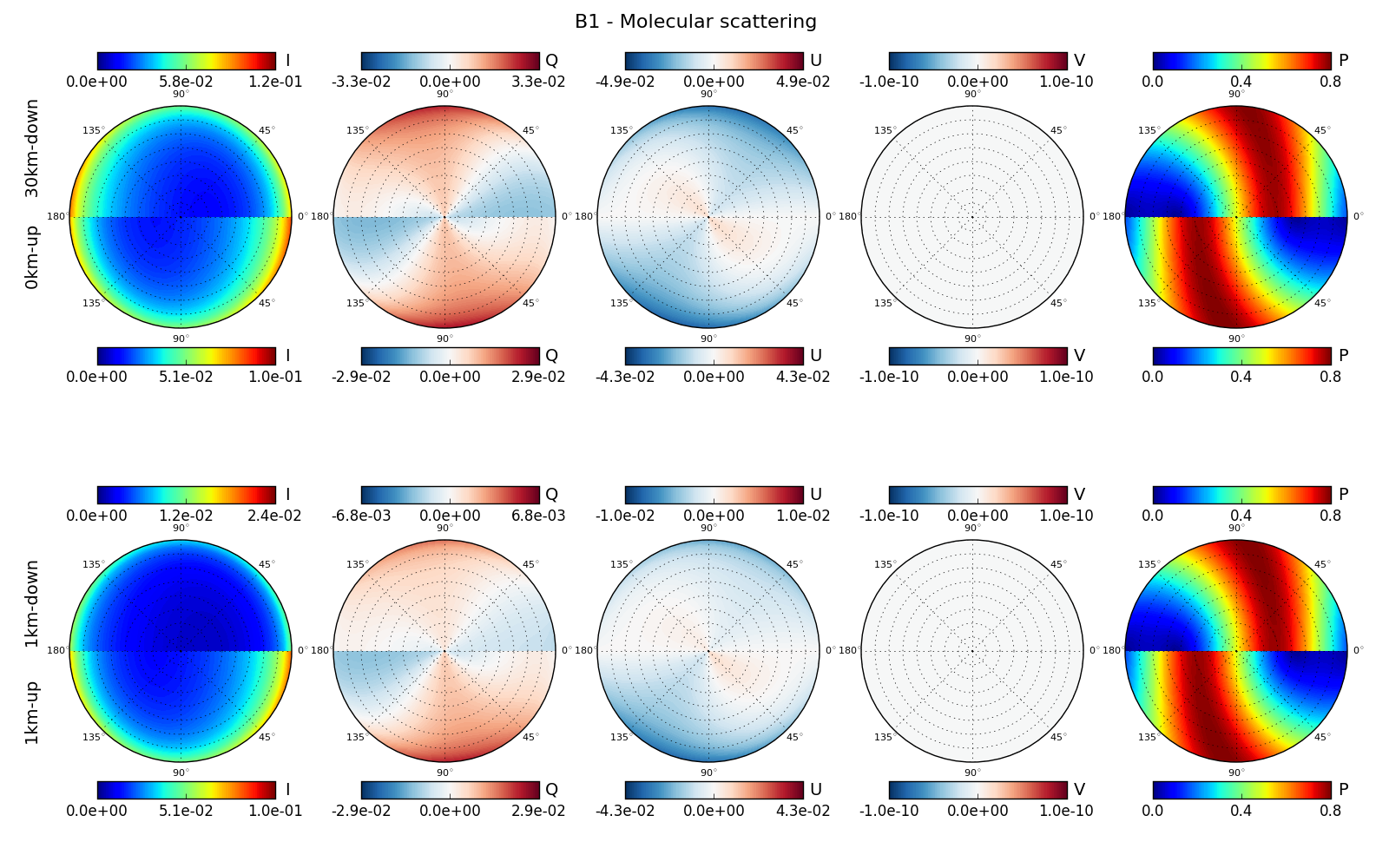
3.3.1 B1 – Rayleigh scattering for a standard atmosphere

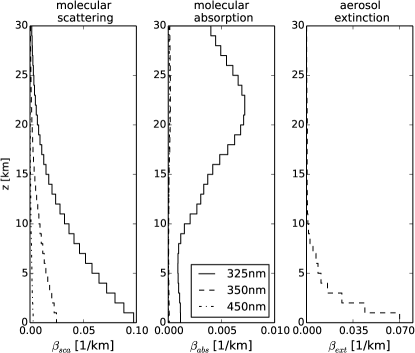
The test case checks whether the discretization of the atmosphere into plane-parallel layers is correctly implemented in the models. The radiance field is calculated at 450 nm taking into account only Rayleigh scattering, i.e. molecular absorption is neglected. The sun position is $(\theta_{0}=60^{\circ},\phi_{0}=0^{\circ})$. The scattering coefficient profile is shown in the left plot of Fig. 6, the dash-dotted line corresponds to 450 nm. The Rayleigh depolarization factor is 0.03. The upper two rows of Fig. 7 show the radiance field at top of atmosphere and surface and at 1 km altitude. As expected the pattern is very similar to the simulation with one layer (see Sec. 3.2.1).

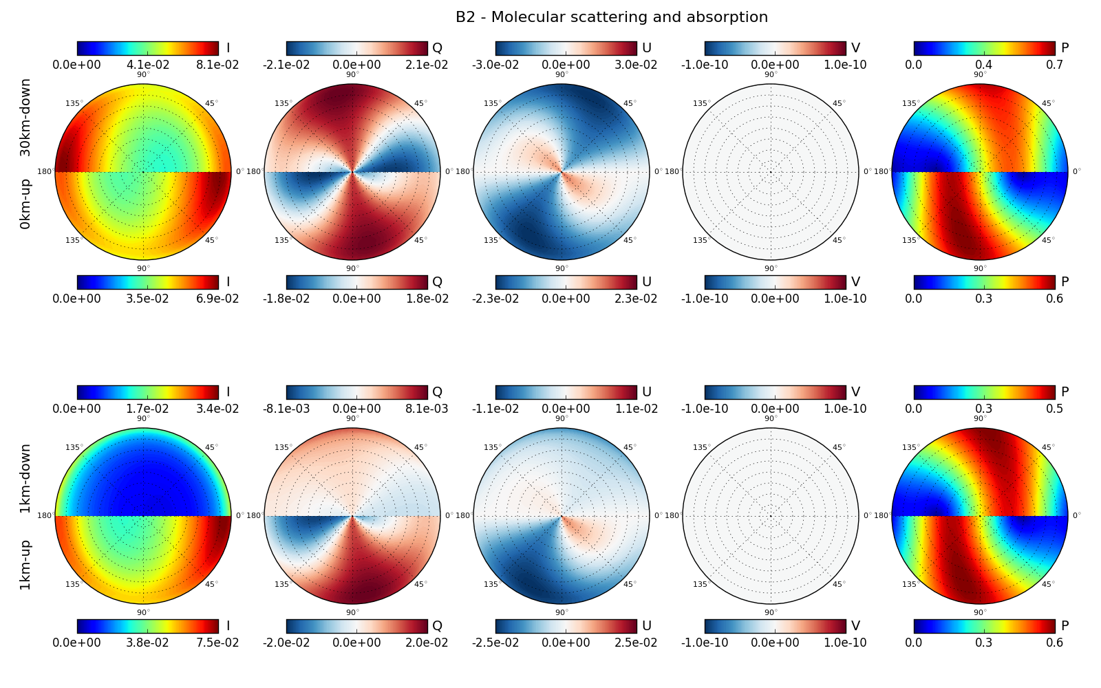
3.3.2 B2 – Rayleigh scattering and absorption for a standard atmosphere

This case checks whether absorption is correctly taken into account. We calculate the radiance field at 325 nm for the US-standard atmosphere. The sun position is $(\theta_{0}=60^{\circ},\phi_{0}=0^{\circ})$. The scattering coefficient profile is shown in the left plot of Fig. 6 and the absorption coefficient profile is shown in the middle plot; generally the solid lines corresponds to 325 nm. Besides the strong absorption at this wavelength due to ozone Rayleigh scattering is also much stronger than at 450 nm. The third and fourth row in Fig. 7 show the radiance field at top of atmosphere, at the surface and at 1 km altitude. All Stokes components show the characteristic Rayleigh scattering pattern as for case B1 (pure Rayleigh scattering). However the degree of polarization is smaller than for case B1.

Figure 7: Radiation fields at surface (0km), top of atmosphere (30km), and at 1 km altitude. The upper two rows correspond to the pure Rayleigh scattering case (B1, see Sec. 3.3.1) and the lower 2 rows are for Rayleigh scattering and absorption (B2, see Sec. 3.3.2). The upper parts of the polar plots are for downlooking directions and the lower parts for uplooking. The Stokes components and the degree of polarization are shown.

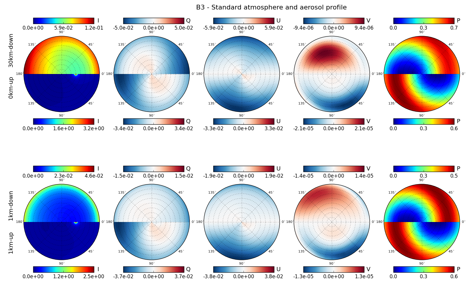
3.3.3 B3 – Aerosol profile and standard atmosphere

Here we check whether the models can correctly handle different atmospheric constituents with similar extinction coefficients in the same layers. We perform simulations at 350 nm for a standard atmosphere including molecular absorption and scattering and additionally an aerosol profile similar to Shettle [1989] with a total optical thickness of 0.2. Molecular absorption and scattering profiles and the aerosol extinction profile are shown in Fig. 6 (dashed lines). We assume spheroidal aerosol partials with the same optical properties as in Sec. 3.2.4. The sun position is $(\theta_{0}=30^{\circ},\phi_{0}=0^{\circ})$. The upper two rows of Fig. 8 show the radiance field at top of atmosphere, at the surface and at 1 km altitude. The total intensity $I$ for up-looking directions is dominated by the forward scattering peak. The polarization pattern is dominated by Rayleigh scattering and the features in the radiation field for test case A4 (layer with aspherical aerosol particles, see Fig. 5), e.g. the two maxima in the degree of polarization or the patterns in $U$ and $V$ in the forward scattering region, are no longer visible. The main effect of aerosol is a decrease in the degree of polarization which is most likely due to the dilution of the strong Rayleigh polarization by the weaker aerosol polarization.

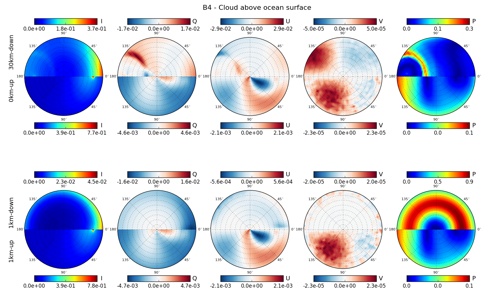
3.3.4 B4 – Cloud above ocean surface

This most sophisticated test case includes a cloud layer embedded in a standard atmosphere above an ocean surface. The calculation is performed at a wavelength of 800 nm, molecular scattering is included, absorption is neglected. The ocean surface is defined as in Sec. 3.2.6, here also we assume a wind speed of 2 m/s and we use 1.33+0$i$ as the refractive index for water. Additionally, a cloud layer with an optical thickness of 5 is included from 2 km to 3 km altitude. The cloud optical properties are the same as in Sec. 3.2.5. The sun position for this case is $(\theta_{0}=60^{\circ},\phi_{0}=0^{\circ})$. The lower two rows of Fig. 8 show the radiance field at top of atmosphere, at the surface and at 1 km altitude. The down-looking radiance field (reflectance) at the top of the atmosphere shows the cloudbow very clearly with high contrast in the degree of polarization, whereas in the total intensity the feature is very weak. The degree of polarization for down-looking directions at 1¨km altitude shows an interesting feature, it is $\sim$90% for a viewing angle of $\sim$53^∘ corresponding to the Brewster angle for the water surface ($\theta_{B}=\arctan(1.33)$). Due to multiple scattering in the cloud layer we get incident radiation on the water surface from all directions. Now the radiation which hits the surface at the Brewster angle is fully polarized after reflection, and the reflected direction is at the same angle, this nicely explains the observed pattern. The “ring” is smeared because the ocean surface with waves is not an ideal mirror. As for the aerosol case the total intensity for the up-looking directions at the surface and at 1 km altitude is dominated by sharp forward scattering peak. The patterns for $Q$ and $U$ for up-looking directions show a characteristic cloud scattering pattern which is very different from the Rayleigh scattering pattern.

Figure 8: Radiation fields at surface (0km), top of atmosphere (30km), and at 1 km altitude. The upper two rows correspond to the case with aerosol profile (B3, see Sec. 3.3.3) and the lower 2 rows are for a cloud layer above an ocean surface (B4, see Sec. 3.3.4). The upper parts of the polar plots are for downlooking directions and the lower parts for uplooking. The Stokes components and the degree of polarization are shown.

4 Model intercomparison

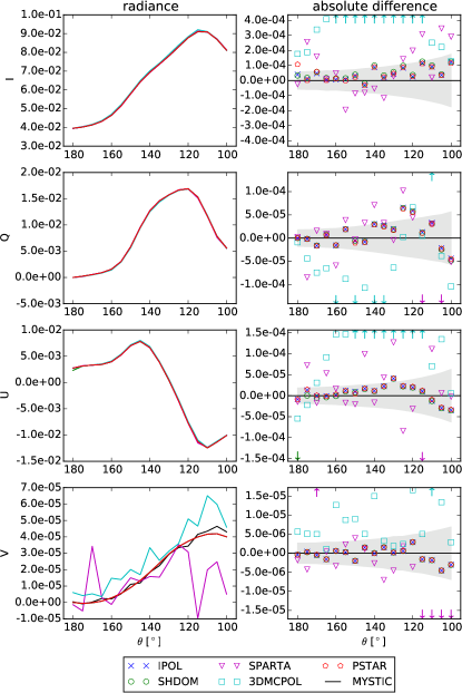
This section presents results of all models for an exemplary selection of viewing angles. For each test case, one or two plots show the simulated Stokes vector and the absolute differences between MYSTIC and IPOL, SPARTA, Pstar, SHDOM, and 3DMCPOL respectively. Out of range values are shown as arrows in the difference plots. Comparison plots for all viewing directions are provided on the IPRT website and as supplementary material.

In order to quantify the level of agreement between the models we calculate the relative root mean square differences $\Delta_{m}$ between MYSTIC and other codes for the full radiation field including all up- and down-looking directions. This yields one representative number for each test case. We define $\Delta_{m}$ for $I$ as follows:

$$\Delta_{m}=\frac{\sqrt{\sum_{i=1}^{N}{\left(I^{i}_{\rm MYSTIC}-I^{i}_{m}\right)^{2}}}}{\sqrt{\sum_{i=1}^{N}{\left(I^{i}_{\rm MYSTIC}\right)^{2}}}}$$ (22)

Here $m$ denotes the radiative transfer model and the summation is done over all $N$ directions, for which the radiation field is calculated. For the other Stokes components $\Delta_{m}$ is calculated accordingly. We look at relative root mean square differences because the Stokes components $Q$, $U$ and $V$ are differences between intensities (see Eq. 1) and for some geometries they have zero or extremely small values. Mean relative differences are therefore not meaningful because relative differences for radiance values very close to zero become very large. A weakness of the definition of $\Delta_{m}$ is that it might be dominated by a few very large differences at specific viewing directions. For cases with strongly peaked phase functions (i.e. cloud cases) $\Delta_{m}$ is dominated by the forward scattering region. Therefore we also calculated $\Delta_{m}$ without the solar aureole region, i.e. directions up to 10^∘ from the sun direction are taken out of the summation in Eq. 22.

4.1 Test cases including a single layer

The relative root mean square differences for the single layer test cases are listed in Table 3, mostly the level of agreement is of the order of 0.1%. For the cloud case A5, the MYSTIC reference results, especially for circular polarization, are more noisy, hence the relative root mean square difference becomes larger although most models still agree perfectly within the expected accuracy range.

model name		A1	A2	A3	A4	A5pp	A5${}^{\rm pp}_{\rm part}$	A5al	A5${}^{\rm al}_{\rm part}$	A6
IPOL	I	0.017	0.009	0.102	0.088	0.183	0.077	0.178	0.075	0.064
	Q	0.024	0.036	0.287	0.028	0.794	0.771	0.816	0.803	0.124
	U	0.029	0.029	0.295	0.034	-	-	1.058	1.039	0.190
	V	-	-	0.800	1.277	-	-	28.313	26.735	-
3DMCPOL	I	0.092	0.010	0.051	0.009	2.432	0.213	2.665	0.197	0.499
	Q	1.681	0.354	0.117	0.041	1.221	0.986	1.094	1.070	2.574
	U	2.129	0.275	0.108	0.061	-	-	1.264	1.198	22.359
	V	-	-	0.519	1.840	-	-	36.313	34.160	-
SPARTA	I	0.088	0.011	0.051	0.027	0.183	0.198	0.213	0.143	0.146
	Q	0.367	0.055	0.120	0.041	2.256	1.725	2.050	2.011	0.152
	U	0.275	0.042	0.084	0.060	-	-	2.928	2.881	0.231
	V	-	-	0.639	2.607	-	-	67.027	64.972	-
SHDOM	I	0.044	0.068	0.111	0.077	3.383	0.077	3.640	0.075	0.089
	Q	0.034	0.233	0.274	0.051	8.735	9.311	0.841	0.805	0.128
	U	0.038	0.112	0.270	0.055	-	-	1.084	1.065	0.195
	V	-	-	0.567	1.818	-	-	28.745	27.062	-
Pstar	I	0.017	0.009	0.100	0.025	0.336	0.081	0.159	0.075	0.100
	Q	0.024	0.036	0.289	0.028	0.809	0.775	0.827	0.811	0.165
	U	0.029	0.029	0.299	0.035	-	-	1.048	1.029	0.273
	V	-	-	0.808	1.278	-	-	28.302	26.732	-

Table 3: Relative root mean square differences $\Delta_{m}$ in per cent between MYSTIC and IPOL, 3DMCPOL, SPARTA, SHDOM and Pstar for the single layer intercomparison cases. For the cloud cases the columns A5${}^{\rm pp}_{\rm part}$ and A5${}^{\rm al}_{\rm part}$ are added which include $\Delta_{m}$ calculated without the solar aureole region, i.e. viewing angles up to 10^∘ from the sun direction are taken out of the summation in Eq. 22.

4.1.1 A1 – Rayleigh scattering

The left plots in Fig. 9 show the Stokes vector calculated at the top of the layer for down-looking directions. The sun is located in the zenith, which means that $U$ is 0. The Rayleigh depolarization factor in this case is 0. The right plots show the absolute differences between the models. The grey area corresponds to two standard deviations (2$\sigma$) of the MYSTIC results, this means that with a probability of 95.4% the difference between the MYSTIC result and the true value lies in the grey area.

Figure 9: Test case A1, Rayleigh scattering layer, depolarization factor 0, sun in the zenith, $\phi$=90^∘. Left: Stokes vector at the top of layer. Right: Absolute difference between individual models and MYSTIC, the grey area corresponds to 2$\sigma$ of the Monte Carlo calculations.

Looking at the left plots, we do not see differences between the models, all lines are on top of each other. The right plots show that the differences between the models are three orders of magnitude smaller than the radiance values. The level of agreement between IPOL and Pstar is even better since the symbols of the two models always lie on top of each other. This is not surprising because the models use the same method. For IPOL, SPARTA and Pstar the differences are centered about 0 and they are well in the 2$\sigma$ range, hence we may conclude that these models agree perfectly with MYSTIC on a very high accuracy level. For $I$ the SHDOM results are slightly smaller than MYSTIC whereas the 3DMCPOL results are slightly larger. For $Q$, 3DMCPOL is slightly smaller than MYSTIC. The difference plots show a similar progression for all models, this is due to statistical noise of the MYSTIC results. The Monte Carlo models SPARTA and 3DMCPOL use a technique to sample all directions based on the same photon paths. In this case the statistical error is the same for all viewing directions whereas for MYSTIC each direction is calculated separately with an independent statistical error.

Figure 10: Test case A1, Rayleigh scattering layer, depolarization factor 0.1, sun at $(\theta_{0}=30^{\circ},\phi_{0}=65^{\circ})$, $\phi$=90^∘. Left: Stokes vector at the surface. Right: Absolute difference between individual models and MYSTIC, the grey area corresponds to 2$\sigma$. Arrows indicate out-of-range values.

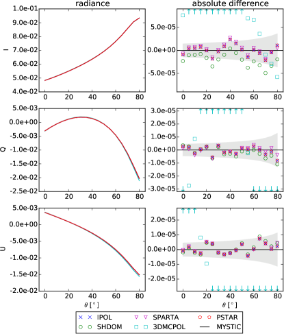
Fig. 10 shows results for a Rayleigh scattering matrix with depolarization factor 0.1. Here the solar zenith angle is 30^∘, hence $Q$ and $U$ are non-zero. In the left plots we see that almost all model results are on top of each other, only the 3DMCPOL values are slightly below the results of the other models. The maximum deviation is about 4% for $Q$, the differences between MYSTIC and 3DMCPOL are mostly out of range in the right plots. This indicates that the depolarization factor in 3DMCPOL is not correctly implemented. The depolarization factor bias observed for 3DMCPOL was not corrected, consequently it has some impacts on the results of the next sections. The models IPOL and Pstar again agree perfectly, as in Fig. 10 the symbols showing the differences to MYSTIC lie on top of each other. The SPARTA results are very close to IPOL and Pstar. The differences between IPOL, Pstar and SPARTA are centered about 0 and well within the 2$\sigma$ range, hence they agree perfectly with MYSTIC. For SHDOM the same is true for $Q$ and $U$, whereas for $I$ SHDOM is systematically slightly smaller than MYSTIC.

Tab. 3 shows that for test case A1, $\Delta_{m}$ is smaller than 0.03% for all Stokes components for the models IPOL, Pstar. Indeed the numbers of $\Delta_{m}$ are exactly the same for IPOL and Pstar which shows that the models use exactly the same method to solve the radiative transfer equation for Rayleigh scattering. For SHDOM $\Delta_{m}$ is smaller than 0.05%, for SPARTA smaller than 0.4% and for 3DMCPOL smaller than 2.1%.

4.1.2 A2 – Rayleigh atmosphere above Lambertian surface

Figure 11: Test case A2, Rayleigh scattering layer (depolarization factor 0.03) above Lambertian surface with albedo 0.3, sun at $(\theta_{0}=50^{\circ},\phi_{0}=0^{\circ})$, $\phi$=45^∘. Left: Stokes vector at top of atmosphere. surface reflection. Right: Absolute difference between individual models and MYSTIC, the grey area corresponds to 2$\sigma$. Arrows indicate out-of-range values.

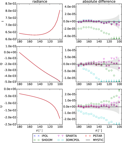
Fig. 11 shows results for the Rayleigh atmosphere above a Lambertian surface. In the radiance plots on the left side we see that all lines are on top of each other. The difference plots show that again, the models IPOL and Pstar agree, their symbols are exactly on top of each other. The differences for IPOL, Pstar and SPARTA scatter around 0 and they mostly lie within the 2$\sigma$ range, hence these models agree perfectly within the expected accuracy of the MYSTIC results. For $I$ the same is true for 3DMCPOL, whereas for $Q$ and $U$ the 3DMCPOL results are systematically smaller than MYSTIC. The reason for this small, but systematic difference could be, as for the case without surface, a slightly different implementation of the Rayleigh depolarization factor which is 0.03 in this case. The SHDOM results are slightly below MYSTIC for $I$ and $Q$ and slightly above for $U$.

Quantitatively we see in Tab. 3 that the level of agreement between MYSTIC and the models IPOL, Pstar and SPARTA is $\Delta_{m}<$0.05% and for SHDOM and 3DMCPOL $\Delta_{m}<$0.35%.

4.1.3 A3 – Spherical aerosol particles

Figure 12: Test case A3, layer with spherical aerosol particles, optical thickness 0.2, sun at $(\theta_{0}=40^{\circ},\phi_{0}=0^{\circ})$, $\phi$=135^∘. Left: Stokes vector at top of atmosphere. Right: Absolute difference between individual models and MYSTIC, the grey area corresponds to 2$\sigma$.

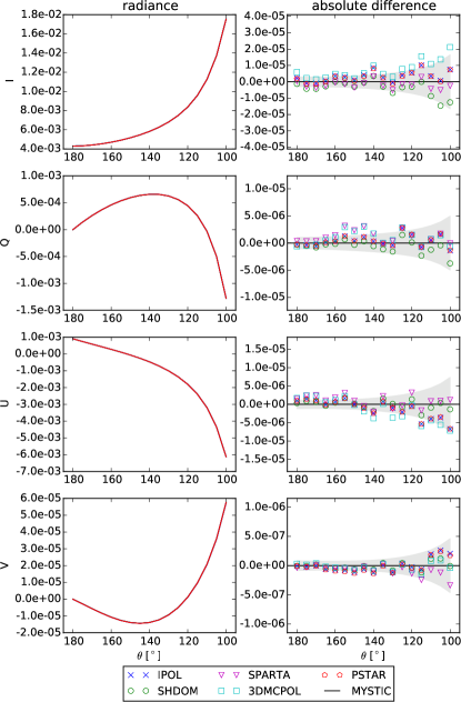
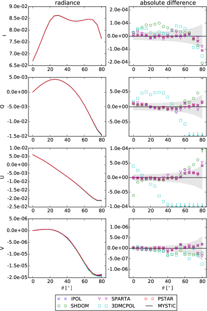
Fig. 12 shows that all models agree very well for the layer with the small spherical aerosol particles. The left side of the plot shows that all models produce the full Stokes vector, also the component for circular polarization $V$ very accurately, all curves are here on top of each other. The difference plots on the right show that the differences for all models lie in the 2$\sigma$ range. For $I$ the 3DMCPOL results seem systematically larger than MYSTIC, although they are still in the 2$\sigma$ range.

The relative root mean square differences are $<$0.3% for $I$, $Q$ and $U$ and $<$0.8% for $V$ (see Tab. 3).

4.1.4 A4 – Spheroidal aerosol particles

Figure 13: Test case A4, layer with spheroidal aerosol particles, optical thickness 0.2, sun at $(\theta_{0}=40^{\circ},\phi_{0}=0^{\circ})$, $\phi$=45^∘. Left: Stokes vector at the top of the atmosphere. Right: Absolute difference between individual models and MYSTIC, the grey area corresponds to 2$\sigma$.

The left plots in Fig. 13 show the Stokes vector at the top of the atmosphere, again all lines are on top of each other. The absolute differences between MYSTIC and all other models are in the 2$\sigma$ range for all Stokes components. The scattering phase function for the particles considered here shows strong forward scattering.

Figure 14: Test case A4, settings as in Fig. 13 but for $\phi$=0^∘. Left: Stokes vector at the surface. Right: Absolute difference between individual models and MYSTIC, the grey area corresponds to 2$\sigma$.

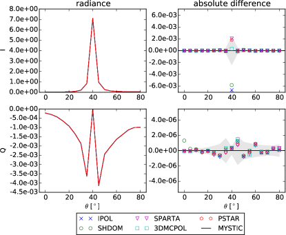
Fig. 14 shows Stokes vector at the surface for a viewing azimuth of 0^∘, for which the $U$ and $V$ are 0. This geometry includes the sun direction and the forward scattering peak. The left plots show, that also the forward scattering peak is calculated accurately by all models. The models 3DMCPOL, Pstar and SPARTA agree to MYSTIC within the 2$\sigma$ range, even in exact forward scattering directions, where SHDOM and IPOL are a little lower (0.1%). For $Q$ all models agree with MYSTIC in the expected 2$\sigma$ range.

Tab. 3 shows that the relative root mean square difference between MYSTIC and all models is 0.09% or better for $I$, $Q$, and $U$. For $V$ the differences are of the order of 1–3%. The absolute value of $V$ is of the order of $10^{-7}$ and the statistical uncertainty of the Monte Carlo results for this small radiances is about 1–3%.

4.1.5 A5 – Liquid water cloud

Figure 15: Test case A5, cloud layer with optical thickness of 5, effective radius of 10, principal plane, sun at $(\theta_{0}=50^{\circ},\phi_{0}=0^{\circ})$. Left: Stokes vector at the surface. Right: Absolute difference between individual models and MYSTIC, the grey area corresponds to 2$\sigma$. A marker is plotted only at every 5^∘, although the simulations were done in 1^∘ steps. Arrows indicate out-of-range values.

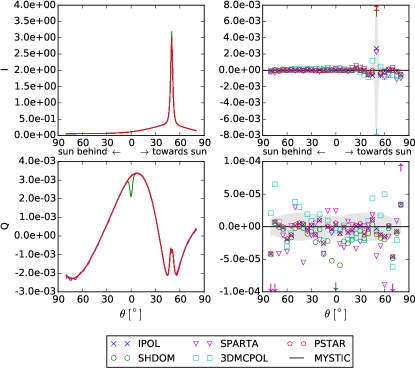
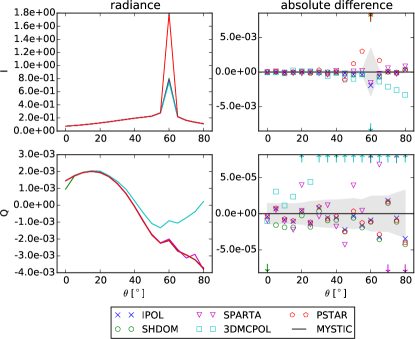
Fig. 15 shows the principal plane. In the region of the forward scattering peak the models IPOL and SPARTA agree to MYSTIC within the expected accuracy (2$\sigma$ of MYSTIC calculation). For 3DMCPOL the value of the forward scattering peak in total intensity $I$ about 3% smaller whereas for Pstar and SHDOM it is larger (about 0.5% and 6% respectively). SHDOM has an artefact in the second Stokes component Q around 0^∘ viewing zenith angle. Further tests have shown that this artefact around 0^∘ and 180^∘ viewing zenith angles occurs only with highly peaked phase functions and are largest for moderate optical depths (there is no artefact for single scattering). The width of the artefact decreases with higher SHDOM angular resolution. The artefact is believed to be a result of a deficiency in the delta-M formulation for polarization.

Figure 16: Test case A5, settings as in Fig: 15 but for “almucantar plane”, viewing zenith angle of 50^∘. Left: Stokes vector at the top of the layer. Right: Absolute difference between individual models and MYSTIC, the grey area corresponds to 2$\sigma$. A marker is plotted only at every 5^∘, although the simulations were done in 1^∘ steps.

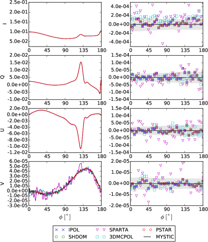
Fig. 16 shows the reflected radiance in the “almucantar” plane, i.e. the viewing zenith angle is constant and corresponds to the solar zenith angle of 50^∘. Here we see clearly that the standard deviation of 3DMCPOL and SPARTA is a little higher than for MYSTIC, therefore several points are outside the 2$\sigma$ range. For SPARTA this is not surprising because it does not use any variance reduction techniques for highly asymmetric scattering phase functions. For the very small Stokes component $V$, all Monte Carlo models are quite noisy, which can be seen in the radiance plot for $V$. Using more photons or including better variance reduction method could decrease the noise. Within the Monte Carlo noise the models agree perfectly.

Tab. 3 shows that the smallest relative root mean square difference is found for IPOL and Pstar, with $\Delta_{m}<$0.4% for $I$ and values about 1% for $Q$ and $U$. For $V$, $\Delta_{m}$ is much larger, about 30%. The reason is the large noise in the MYSTIC calculations. Except for $V$, a good agreement (within the range of 0.2%-3%) is found for the models 3DMCPOL and SPARTA. For SHDOM, $\Delta_{m}$ for $Q$ is dominated by the artefact mentioned before. Without the specific directions (forward scattering and 0^∘ viewing zenith angle), SHDOM also agrees perfectly to all other models (see column A5${}^{al}_{part}$ in Tab. 3).

4.1.6 A6 – Rayleigh atmosphere above ocean surface

Figure 17: Test case A6, Rayleigh scattering layer above ocean surface with windspeed of 2 m/s, sun at $(\theta_{0}=45^{\circ},\phi_{0}=0^{\circ})$, $\phi$=10^∘. Left: Stokes vector at top of atmosphere. Right: Absolute difference between individual models and MYSTIC, the grey area corresponds to 2$\sigma$. Arrows indicate out-of-range values.

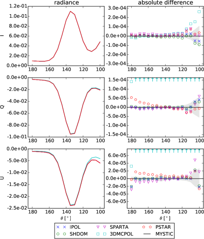
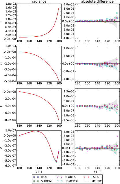
Fig. 17 shows the reflected Stokes vector for the Rayleigh scattering layer above the ocean surface. All models produce the sunglint and the models MYSTIC, IPOL, SHDOM and SPARTA agree very well. For Pstar, we see a small bias for all Stokes components in the shown geometry. The 3DMCPOL results show larger deviations for all Stokes components due to an error in the code which has not been discovered so far.

The numbers in Tab. 3 show that the models IPOL, SPARTA, Pstar and SHDOM agree very well to MYSTIC with $\Delta_{m}<\sim$0.3%. The 3DMCPOL results are inaccurate especially for $U$.

4.2 Test cases with realistic atmospheric profiles

For the multi-layer test cases, the radiation fields have been calculated at the surface, at the top of the atmosphere and inside the atmosphere at an altitude of 1 km. However, at present time only MYSTIC, SHDOM and Pstar are capable to calculate the radiance field inside the atmosphere. The relative root mean square differences for the multi layer test cases are listed in Table 4, the details are discussed in the following sections.

model name		B1	B2	B3	B3part	B4	B4part
IPOL	I	0.016	0.012	0.060	0.014	0.111	0.091
	Q	0.024	0.023	0.049	0.034	0.575	0.472
	U	0.019	0.019	0.043	0.026	0.601	0.478
	V	-	-	1.489	1.073	19.377	15.091
3DMCPOL	I	0.033	1.387	0.040	0.064	1.152	0.727
	Q	0.558	0.975	1.296	1.261	27.614	14.805
	U	0.505	0.517	1.037	0.979	5.965	5.878
	V	-	-	4.347	3.833	94.928	62.132
SPARTA	I	0.020	0.013	0.055	0.026	0.344	0.326
	Q	0.030	0.029	0.071	0.045	3.710	2.699
	U	0.023	0.023	0.064	0.036	4.368	2.856
	V	-	-	1.982	1.439	182.181	88.770
SHDOM	I	0.052	0.054	0.426	0.069	1.059	0.109
	Q	0.068	0.071	0.148	0.085	2.377	1.654
	U	0.040	0.054	0.136	0.057	3.846	2.153
	V	-	-	2.567	1.548	23.672	19.700
Pstar	I	0.017	0.013	0.154	0.017	34.947	0.182
	Q	0.025	0.026	0.052	0.039	0.644	0.579
	U	0.020	0.021	0.047	0.031	2.583	2.661
	V	-	-	1.553	1.127	23.695	19.730

Table 4: Relative root mean square differences $\Delta_{m}$ in per cent between MYSTIC and IPOL, 3DMCPOL, SPARTA, SHDOM and Pstar for the multi-layer intercomparison cases. For B3_part and B4_part the solar aureole region is taken out of the calculation of $\Delta_{m}$, i.e. viewing angles up to 10^∘ from the sun direction are taken out of the summation in Eq. 22.

4.2.1 B1 – Rayleigh scattering for a standard atmosphere

Figure 18: Test case B1, US-standard atmosphere, 450 nm, no absorption, sun at $(\theta_{0}=60^{\circ},\phi_{0}=0^{\circ})$, $\phi$=90^∘. Left: Stokes vector at the surface. Right: Absolute difference between individual models and MYSTIC, the grey area corresponds to 2$\sigma$. Arrows indicate out-of-range values.

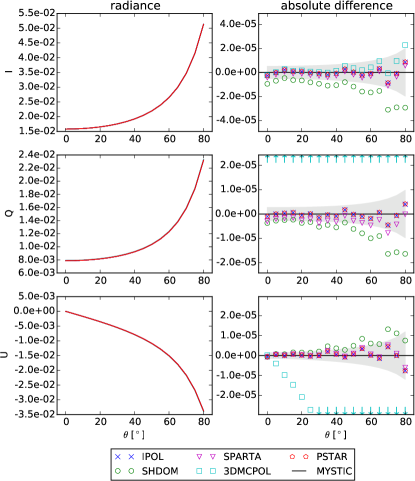
Fig. 18 shows the results for a multi-layer atmosphere with pure Rayleigh scattering. As for the 1-layer case, we find a very good agreement between all models for pure Rayleigh scattering. The models IPOL, SPARTA and Pstar agree among each other. SHDOM is slightly smaller for $I$ and $Q$ and slightly larger for $U$. 3DMCPOL shows small but systematic deviations, which might again be due to a different implementation of the Rayleigh depolarization factor, which was set to 0.03 in this test case.

Tab. 4 shows that relative root mean square deviations are mostly smaller than 0.05% between MYSTIC and IPOL, SPARTA, SHDOM, and Pstar respectively. For 3DMCPOL, $\Delta_{m}$ is 0.03% for $I$ and about 0.5% for $Q$ and $U$.

4.2.2 B2 – Rayleigh scattering and absorption for a standard atmosphere

Figure 19: Test case B2, US-standard atmosphere, scattering an absorption, 325 nm, sun at $(\theta_{0}=60^{\circ},\phi_{0}=0^{\circ})$, $\phi$=45^∘. Left: Stokes vector at the surface. Right: Absolute difference between individual models and MYSTIC, the grey area corresponds to 2$\sigma$. Arrows indicate out-of-range values.

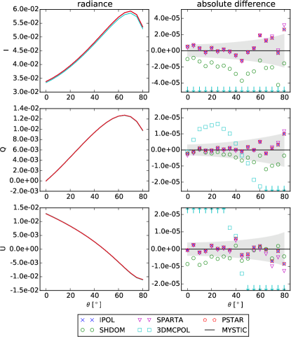
Fig. 19 shows the results for the US-standard atmosphere simulated at 325 nm, where absorption has been included. The models IPOL, SPARTA and Pstar agree to MYSTIC within two standard deviations. The SHDOM results show a small bias, for $I$ they are slightly smaller than the MYSTIC results. The 3DMCPOL results differ by more than 1%.

In Tab. 4 we see that relative root mean square deviations are as for test case B1 mostly smaller than 0.05% between MYSTIC and IPOL, SPARTA, SHDOM, and Pstar respectively. For 3DMCPOL, $\Delta_{m}$ is in the range of 0.5%–1.5% for all Stokes components.

4.2.3 B3 – Aerosol profile and standard atmosphere

Figure 20: Test case B3, US-standard atmosphere, 350 nm, aerosol profile, spheroidal particles, sun at $(\theta_{0}=30^{\circ},\phi_{0}=0^{\circ})$, $\phi$=45^∘. Left: Stokes vector at the surface. Right: Absolute difference between individual models and MYSTIC, the grey area corresponds to 2$\sigma$. Arrows indicate out-of-range values.

For the standard atmosphere including a realistic aerosol profile again all models agree very well. Fig. 20 shows that deviations between MYSTIC and IPOL, SPARTA and Pstar are again within the expected uncertainty for most angles. There are some tiny deviations for SHDOM. 3DMCPOL again shows small systematic deviations, especially for $Q$ and $U$.

The relative root mean square deviations from MYSTIC (Tab. 4) are smaller than 0.07% for $I$, $Q$ and $U$ for the models IPOL and SPARTA. For Pstar and SHDOM, the differences are slightly larger (up to 0.4%). $\Delta_{m}$ is about 1.5% for $V$ for IPOL and Pstar. This larger deviation is due to an increased relative standard deviation of MYSTIC, because $V$ is four orders of magnitude smaller than $Q$ and $U$. For 3DMCPOL, $\Delta_{m}\sim$0.04% for $I$, of the order of 1% for $Q$ and $U$ and 4% for $V$.

4.2.4 B4 – Cloud above ocean surface

Figure 21: Test case B4, US-standard atmosphere, 800 nm, ocean surface, cloud layer with optical thickness of 5, sun at $(\theta_{0}=60^{\circ},\phi_{0}=0^{\circ})$, $\phi$=0^∘. Left: Stokes vector at the surface. Right: Absolute difference between individual models and MYSTIC, the grey area corresponds to 2$\sigma$. Arrows indicate out-of-range values.

Figure 22: Test case B4, settings as Fig. 21 but for $\phi$=135^∘. Left: Stokes vector at 1 km altitude for downward viewing directions. Right: Absolute difference between individual models and MYSTIC, the grey area corresponds to 2$\sigma$. Arrows indicate out-of-range values.

Figure 23: Test case B4, settings as Fig. 22. Left: Stokes vector at the top of the atmosphere. Right: Absolute difference between individual models and MYSTIC, the grey area corresponds to 2$\sigma$. Arrows indicate out-of-range values.

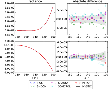
For the most demanding case of a cloud layer above an ocean surface embedded in a Rayleigh atmosphere we find the largest differences between the models. Figs. 21–23 show the radiance field and the differences between the models.

Fig. 21 shows the radiance field for a viewing azimuth angle of 0^∘ at the surface. Here all models agree quite well when the forward scattering direction is excluded, only the 3DMCPOL result for $Q$ is different from other models. This difference is mainly due to the error in the implementation of surface reflection in 3DMCPOL. Within the 2$\sigma$ range the models Pstar, IPOL and SHDOM mostly agree to MYSTIC. There is one outlier in the SHDOM results for $Q$ at a viewing zenith angle of 0^∘. In the exact forward direction Pstar is more than a factor of 2 larger than the other models. This is because Pstar uses a relatively small number of streams, i.e. 60 for this case. The result in exact forward direction improves by increasing the number of streams. The value of the forward scattering peak agrees for MYSTIC, IPOL and SPARTA.

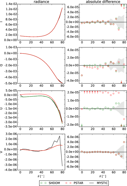
Fig. 22 shows the radiance field at a viewing azimuth angle of 135^∘ for down-looking directions at 1 km altitude, below the cloud layer, We find that the models MYSTIC, SHDOM and Pstar agree for $I$, $Q$ and $V$. For $U$ SHDOM and MYSTIC are negative whereas Pstar is slightly positive.

Fig. 23 shows the radiance field at a viewing azimuth angle of 135^∘ for down-looking directions at the top of the atmosphere, where we see part of the cloudbow. IPOL, SHDOM and Pstar mostly agree to MYSTIC within the 2$\sigma$ range. SHDOM again shows an outlier at 180^∘viewing zenith angle. SPARTA results are more noisy than MYSTIC but there are no obvious systematic differences and within the uncertainty the models agree. For 3DMCPOL the differences are a bit larger and systematic, e.g. for $I$ the 3DMCPOL results are systematically larger than other model results.

Tab. 4 shows that the relative root mean square difference between MYSTIC and all other models is very small for $I$, the largest difference is 0.7%. For $Q$ and $U$, $\Delta_{m}$ is smaller than 0.6% for IPOL, 1–4% for SHDOM, Pstar and SPARTA, and 5–27% for 3DMCPOL. For $V$, $\Delta_{m}$ is about 20% for IPOL, SHDOM and Pstar; this large value is due to the noisy MYSTIC result. Since 3DMCPOL and SPARTA are more noisy than MYSTIC the values are even larger.

5 Conclusion and Outlook

Overall, we found a very good agreement between all models and for the test cases of this intercomparison project. The achieved level of agreement is very high, for cases without clouds the relative root mean square difference is mostly below 0.05% for total intensity and linear polarization. However some significant deviations were found: for non-zero depolarization factors, for ocean reflection, and for simulations including cloud droplets. For these settings some of the models need to be corrected or improved.

For all single layer calculations we found an agreement between the models MYSTIC, IPOL, SPARTA and Pstar. SHDOM also agrees for all cases and almost all viewing directions, but for the cloud layer cases it shows artefacts at a few specific viewing directions. 3DMCPOL agrees well for Rayleigh scattering with depolarization factor set to 0, for the Lambertian surface, and for aerosol and cloud cases. There are small differences when the depolarization factor is non-zero and also for the case with ocean reflectance matrix, for these two cases we may conclude that 3DMCPOL is not consistent with other models and should be corrected.

For the multi-layer cases the radiance fields at the surface and at the top of the atmosphere were provided by all participants. We again find a perfect agreement between MYSTIC, IPOL, SPARTA and with a few exceptions SHDOM, which shows artefacts at a few specific angles for the cloud case, in particular at viewing angles of 0^∘and 180^∘. Pstar agrees for all cases except the last one with ocean reflectance matrix and cloud layer, where we find small deviations at specific geometries for the $U$ component of the Stokes vector. 3DMCPOL shows small differences for all cases due to the non-zero depolarization factor of 0.03 which was used for all multi-layer cases. Larger differences appear when absorption is taken into account, here the 3DMCPOL model should be improved. Also for the cloud layer above ocean surface we find larger differences, as expected because we have already seen these differences in the single layer case with ocean reflectance matrix.

As benchmark we provide the MYSTIC results, which agree to IPOL and SPARTA for the delivered cases at the surface and the top of the atmosphere. MYSTIC also agrees to SHDOM for most viewing directions, the exceptions are obviously due to artefacts in SHDOM at specific angles. Also it agrees to Pstar for cases without ocean reflectance matrix. Along with the radiance data we provide the standard deviations which are helpful when developers want to use the benchmark data for testing their models.

The detailed setup for all cases, the benchmark results as well as plots showing model results of all cases are publically available at the IPRT website (http://www.meteo.physik.uni-muenchen.de/~iprt).

The next phase of the intercomparison project will start in spring 2015. We will then focus on three-dimensional scenarios including clouds and aerosols.

References

- Deschamps et al. [1994] P.-Y. Deschamps, F.-M. Breon, M. Leroy, A. Podaire, A. Bricaud, J.-C. Buriez, G. Seze, The POLDER mission: instrument characteristics and scientific objectives, IEEE Transactions on Geoscience and Remote Sensing 32 (1994) 598–615, doi:10.1109/36.297978.
- Kuze et al. [2009] A. Kuze, H. Suto, M. Nakajima, T. Hamazaki, Thermal and near infrared sensor for carbon observation Fourier-transform spectrometer on the Greenhouse Gases Observing Satellite for greenhouse gases monitoring, Appl. Opt. 48 (2009) 6716–6733.
- Wielicki et al. [2013] B. A. Wielicki, D. F. Young, M. G. Mlynczak, K. J. Thome, S. Leroy, J. Corliss, J. G. Anderson, C. O. Ao, R. Bantges, F. Best, K. Bowman, H. Brindley, J. J. Butler, W. Collins, J. A. Dykema, D. R. Doelling, D. R. Feldman, N. Fox, X. Huang, R. Holz, Y. Huang, Z. Jin, D. Jennings, D. G. Johnson, K. Jucks, S. Kato, D. B. Kirk-Davidoff, R. Knuteson, G. Kopp, D. P. Kratz, X. Liu, C. Lukashin, A. J. Mannucci, N. Phojanamongkolkij, P. Pilewskie, V. Ramaswamy, H. Revercomb, J. Rice, Y. Roberts, C. M. Roithmayr, F. Rose, S. Sandford, E. L. Shirley, W. L. S. Sr., B. Soden, P. W. Speth, W. Sun, P. C. Taylor, D. Tobin, X. Xiong, Achieving climate change absolute accuracy in orbit, Bulletin of the American Meteorological Society 94 (2013) 1519–1539, doi:http://dx.doi.org/10.1175/BAMS-D-12-00149.1.
- Liu and Voss [1997] Y. Liu, K. Voss, Polarized radiance distribution measurement of skylight. II. Experiment and data, Appl. Opt. 36 (33) (1997) 8753–8764.
- Kreuter et al. [2009] A. Kreuter, M. Zangerl, M. Schwarzmann, M. Blumthaler, All-sky imaging: a simple, versatile system for atmospheric research, Appl. Opt. 48 (6) (2009) 1091–1097.
- Cairns et al. [1999] B. Cairns, E. E. Russell, L. D. Travis, Research Scanning Polarimeter: calibration and ground-based measurements, in: Proceedings of SPIE - The International Society for Optical Engineering, vol. 3754, 186–196, 1999.
- Cairns et al. [2003] B. Cairns, E. Russell, J. LaVeigne, P. Tennant, Research scanning polarimeter and airborne usage for remote sensing of aerosols, in: Proceedings of SPIE - The International Society for Optical Engineering, vol. 5158, 33–44, 2003.
- Diner et al. [2012] D. J. Diner, F. Xu, J. V. Martonchik, B. E. Rheingans, S. Geier, V. M. Jovanovic, A. Davis, R. A. Chipman, S. C. McClain, Exploration of a polarized surface bidirectional reflectance model using the ground-based multiangle spectropolarimetric imager, Atmosphere 3 (2012) 591–619, doi:doi:10.3390/atmos3040591.
- aur [2008] Multidirectional visible and shortwave infrared polarimeter for atmospheric aerosol and cloud observation: OSIRIS (Observing System Including PolaRisation in the Solar Infrared Spectrum), vol. 7149, doi:10.1117/12.806421, URL http://dx.doi.org/10.1117/12.806421, 2008.
- Li et al. [2014] L. Li, Z. Li, K. Li, L. Blarel, M. Wendisch, A method to calculate Stokes parameters and angle of polarization of skylight from polarized {CIMEL} sun/sky radiometers, Journal of Quantitative Spectroscopy and Radiative Transfer 149 (0) (2014) 334 – 346, ISSN 0022-4073, doi:%**** ̵emde˙iprt˙phaseA.bbl ̵Line ̵125 ̵****http://dx.doi.org/10.1016/j.jqsrt.2014.09.003, URL http://www.sciencedirect.com/science/article/pii/S0022407314003744.
- Coulson et al. [1960] K. L. Coulson, J. V. Dave, Z. Sekera, Tables Related to Radiation Emerging from a Planetary Atmosphere with Rayleigh Scattering, University of California Press, 1960.
- Nataraj et al. [2009] V. Nataraj, K.-F. Li, Y. I. Young, Rayleigh scattering in planetary atmospheres: corrected tables through accurate computation of X and Y functions, Astrophysical Journal 691 (2009) 1909–1920.
- de Haan et al. [1987] J. F. de Haan, P. B. Bosma, J. W. Hovenier, The adding method for multiple scattering calculations of polarized light, Astronomy and Astrophysics 183 (1987) 371–391.
- Wauben et al. [1994] W. M. F. Wauben, J. F. de Haan, J. W. Hovenier, A method for computing visible and infrared polarized monochromatic radiation in planetary atmospheres, Astron. Astrophys. 282 (1994) 277–290.
- Garcia and Siewert [1989] R. D. M. Garcia, C. Siewert, The FN method for radiative transfer models that include polarization effects, J. Quant. Spectrosc. Radiat. Transfer 41 (2) (1989) 117–145.
- Kokhanovsky et al. [2010] A. A. Kokhanovsky, V. P. Budak, C. Cornet, M. Duan, C. Emde, I. L. Katsev, D. A. Klyukov, S. V. Korkin, L. C-Labonnote, B. Mayer, Q. Min, T. Nakajima, Y. Ota, A. S. Prikhach, V. V. Rozanov, T. Yokota, E. P. Zege, Benchmark results in vector atmospheric radiative transfer, J. Quant. Spectrosc. Radiat. Transfer 111 (12-13) (2010) 1931–1946.
- Cornet et al. [2010] C. Cornet, L. C-Labonnote, F. Szczap, Three-dimensional polarized Monte Carlo atmospheric radiative transfer model (3DMCPOL): 3D effects on polarized visible reflectances of a cirrus cloud, J. Quant. Spectrosc. Radiat. Transfer 111 (1) (2010) 174 – 186, ISSN 0022-4073, doi:http://dx.doi.org/10.1016/j.jqsrt.2009.06.013.
- Fauchez et al. [2014] T. Fauchez, C. Cornet, F. Szczap, P. Dubuisson, T. Rosambert, Impact of cirrus clouds heterogeneities on top-of-atmosphere thermal infrared radiation, Atmos. Chem. Phys. 14 (11) (2014) 5599–5615, doi:10.5194/acp-14-5599-2014, URL http://www.atmos-chem-phys.net/14/5599/2014/.
- Mayer [2009] B. Mayer, Radiative transfer in the cloudy atmosphere, European Physical Journal Conferences 1 (2009) 75–99.
- Emde et al. [2010] C. Emde, R. Buras, B. Mayer, M. Blumthaler, The impact of aerosols on polarized sky radiance: model development, validation, and applications, Atmos. Chem. Phys. 10 (2) (2010) 383–396.
- Ota et al. [2010] Y. Ota, A. Higurashi, T. Nakajima, T. Yokota, Matrix formulations of radiative transfer including the polarization effect in a coupled atmosphere-ocean system, Journal of Quantitative Spectroscopy and Radiative Transfer 111 (6) (2010) 878–894.
- Evans [1998] K. F. Evans, The spherical harmonics discrete ordinate method for three–dimensional atmospheric radiative transfer, J. Atmos. Sci. 55 (1998) 429–446.
- Barlakas et al. [2014] V. Barlakas, A. Macke, M. Wendisch, A. Ehrlich, Implementation of polarization in a 3D Monte Carlo Radiative Transfer Model, Wissenschaftliche Mitteilungen aus dem Institut für Meteorologie der Universität Leipzig 52 (2014) 1–14.
- Marshak and Davis [2005] A. Marshak, A. Davis, 3D Radiative Transfer in Cloudy Atmospheres, Springer, iSBN-13 978-3-540-23958-1, 2005.
- Potter [1970] J. Potter, Delta function approximation in radiative transfer theory, Journal of the Atmospheric Sciences 27 (6) (1970) 943–949.
- Buras and Mayer [2011] R. Buras, B. Mayer, Efficient unbiased variance reduction techniques for Monte Carlo simulations of radiative transfer in cloudy atmospheres: The solution, J. Quant. Spectrosc. Radiat. Transfer 112 (3) (2011) 434–447.
- Partain et al. [2000] P. T. Partain, A. K. Heidinger, G. L. Stephens, High spectral resolution atmospheric radiative transfer: Application of the equivalence theorem, Journal of Geophysical Research: Atmospheres 105 (D2) (2000) 2163–2177, ISSN 2156-2202, doi:10.1029/1999JD900328, URL http://dx.doi.org/10.1029/1999JD900328.
- Emde et al. [2011] C. Emde, R. Buras, B. Mayer, ALIS: An efficient method to compute high spectral resolution polarized solar radiances using the Monte Carlo approach, J. Quant. Spectrosc. Radiat. Transfer 112 (10) (2011) 1622–1631.
- Cornet et al. [2013] C. Cornet, F. Szczap, L. C.-Labonnote, T. Fauchez, F. Parol, F. Thieuleux, J. Riedi, P. Dubuisson, N. Ferlay, Evaluation of cloud heterogeneity effects on total and polarized visible radiances as measured by POLDER/PARASOL and consequences for retrieved cloud properties, AIP Conference Proceedings 1531 (1) (2013) 99–102, doi:http://dx.doi.org/10.1063/1.4804717, URL http://scitation.aip.org/content/aip/proceeding/aipcp/10.1063/1.4804717.
- Waquet et al. [2013] F. Waquet, C. Cornet, J.-L. Deuzé, O. Dubovik, F. Ducos, P. Goloub, M. Herman, T. Lapyonok, L. C. Labonnote, J. Riedi, D. Tanré, F. Thieuleux, C. Vanbauce, Retrieval of aerosol microphysical and optical properties above liquid clouds from POLDER/PARASOL polarization measurements, Atmospheric Measurement Techniques 6 (4) (2013) 991–1016, doi:10.5194/amt-6-991-2013, URL http://www.atmos-meas-tech.net/6/991/2013/.
- Fauchez et al. [2015] T. Fauchez, P. Dubuisson, C. Cornet, F. Szczap, A. Garnier, J. Pelon, K. Meyer, Impacts of cloud heterogeneities on cirrus optical properties retrieved from space-based thermal infrared radiometry, Atmos. Meas. Tech. 8 (2) (2015) 633–647, doi:10.5194/amt-8-633-2015, URL http://www.atmos-meas-tech.net/8/633/2015/.
- Hovenier et al. [2004] J. Hovenier, C. van der Mee, H. Domke, Transfer of polarized light in planetary atmospheres. Basic concepts and practical methods, Kluwer Academic Publishers, 2004.
- Chalhoub and Garcia [2000] E. S. Chalhoub, R. D. M. Garcia, The equivalence between two techniques of angular interpolation for the discrete-ordinates method, J. Quant. Spectrosc. Radiat. Transfer 64 (2000) 517–535.
- Karp et al. [1980] A. H. Karp, J. Greenstadt, J. A. Fillmore, Radiative transfer through an arbitrary thick scattering atmosphere, J. Quant. Spectrosc. Radiat. Transfer 24 (1980) 391–406.
- Nakajima and Tanaka [1986] T. Nakajima, M. Tanaka, Matrix formulations for the transfer of solar radiation in a plane-parallel scattering atmosphere, J. Quant. Spectrosc. Radiat. Transfer 35 (1) (1986) 13–21.
- Plass et al. [1973] G. N. Plass, G. W. Kattawar, F. E. Catchings, Matrix operator theroy of radiative transfer 1: Rayleigh scattering, Appl. Opt. 12 (1973) 314–329.
- Korkin et al. [2012] S. V. Korkin, A. I. Lyapustin, V. V. Rozanov, Modifications of discrete ordinate method for computations with high scattering anisotropy: comparative analysis, J. Quant. Spectrosc. Radiat. Transfer 113 (2012) 2040–2048.
- Rozanov and Lyapustin [2010] V. V. Rozanov, A. I. Lyapustin, Similarity of radiative transfer equation: error analysis of phase function truncation techniques, J. Quant. Spectrosc. Radiat. Transfer 111 (2010) 1964–1979.
- Korkin et al. [2013] S. V. Korkin, A. I. Lyapustin, V. V. Rozanov, APC: a new code for atmospheric polarization computations, J. Quant. Spectrosc. Radiat. Transfer 127 (2013) 1–11.
- Evans and Stephens [1991] K. F. Evans, G. L. Stephens, A new polarized atmospheric radiative transfer model, J. Quant. Spectrosc. Radiat. Transfer 46 (1991) 413–423.
- Rozanov et al. [2013] V. V. Rozanov, A. V. Rozanov, A. A. Kokhanovsky, J. P. Burrows, Radiative transfer through terrestrial atmosphere and ocean: software package SCIATRAN, J. Quant. Spectrosc. Radiat. Transfer 133 (2013) 13–71.
- Lyapustin [2005] A. I. Lyapustin, Radiative transfer code SHARM for atmospheric and terrestrial applications, Applied Optics 44 (36) (2005) 7764–7772.
- Mayer and Kylling [2005] B. Mayer, A. Kylling, Technical note: The libRadtran software package for radiative transfer calclations – description and examples of use, Atmos. Chem. Phys. 5 (2005) 1855–1877.
- Klinger and Mayer [2014] C. Klinger, B. Mayer, Three-dimensional Monte Carlo calculation of atmospheric thermal heating rates, J. Quant. Spectrosc. Radiat. Transfer 144 (0) (2014) 123–136.
- Davis et al. [2013] A. B. Davis, M. J. Garay, F. Xu, Z. Qu, C. Emde, 3D radiative transfer effects in multi-angle/multispectral radio-polarimetric signals from a mixture of clouds and aerosols viewed by a non-imaging sensor, Proc. SPIE 8873 (2013) 887309–887309–18, doi:10.1117/12.2023733.
- Bugliaro et al. [2011] L. Bugliaro, T. Zinner, C. Keil, B. Mayer, R. Hollmann, M. Reuter, W. Thomas, Validation of cloud property retrievals with simulated satellite radiances: a case study for SEVIRI, Atmos. Chem. Phys. 11 (12) (2011) 5603–5624, doi:10.5194/acp-11-5603-2011, URL http://www.atmos-chem-phys.net/11/5603/2011/.
- Sumińska-Ebersoldt et al. [2012] O. Sumińska-Ebersoldt, R. Lehmann, T. Wegner, J.-U. Grooß, E. Hösen, R. Weigel, W. Frey, S. Griessbach, V. Mitev, C. Emde, C. M. Volk, S. Borrmann, M. Rex, F. Stroh, M. von Hobe, ClOOCl photolysis at high solar zenith angles: analysis of the RECONCILE self-match flight, Atmospheric Chemistry and Physics 12 (3) (2012) 1353–1365, doi:10.5194/acp-12-1353-2012, URL http://www.atmos-chem-phys.net/12/1353/2012/.
- Emde and Mayer [2007] C. Emde, B. Mayer, Simulation of solar radiation during a total solar eclipse: A challenge for radiative transfer, Atmos. Chem. Phys. 7 (2007) 2259–2270.
- Marchuk et al. [1980] G. I. Marchuk, G. A. Mikhailov, M. A. Nazaraliev, The Monte Carlo methods in atmospheric optics, Springer Series in Optical Sciences, Berlin: Springer, 1980.
- Collins et al. [1972] D. G. Collins, W. G. Blättner, M. B. Wells, H. G. Horak, Backward Monte Carlo calculations of the polarization characteristics of the radiation emerging from spherical-shell atmospheres., Appl. Opt. 11 (1972) 2684–2696.
- Fukuda et al. [2013] S. Fukuda, T. Nakajima, H. Takenaka, A. Higurashi, N. Kikuchi, T. Y. Nakajima, H. Ishida, New approaches to removing cloud shadows and evaluating the 380 nm surface reflectance for improved aerosol optical thickness retrievals from the GOSAT/TANSO-Cloud and Aerosol Imager, J. Geophys. Res. 118 (2013JD020090).
- Murakami and Dupouy [2013] H. Murakami, C. Dupouy, Atmospheric correction and inherent optical property estimation in the southwest New Caledonia lagoon using AVNIR-2 high-resolution data, Appl. Opt. 53 (182–198).
- Nakajima and Tanaka [1988] T. Nakajima, M. Tanaka, Algorithms for radiative intensity calculations in moderately thick atmospheres using a truncation approximation, J. Qunat. Spectrosc. Radiat. Transfer 40 (1) (1988) 51–69.
- Ruggaber et al. [1994] A. Ruggaber, R. Dlugi, T. Nakajima, Modelling radiation quantities and photolysis frequencies in the troposphere, Journal of Atmospheric Chemistry 18 (2) (1994) 171–210.
- Pincus and Evans [2009] R. P. Pincus, K. F. Evans, Computational cost and accuracy in calculating three-dimensional radiative transfer: Results for new implementations of Monte Carlo and SHDOM, J. Atmos. Sci. 66 (2009) 3131–3146.
- Doicu et al. [2013] A. Doicu, D. Efremenko, T. Trautmann, A multi-dimensional vector spherical harmonics discrete ordinate method for atmospheric radiative transfer, J. Quant. Spectrosc. Radiat. Transfer 118 (2013) 121–131.
- Mishchenko and Travis [1997] M. I. Mishchenko, L. D. Travis, Satellite retrieval of aerosol properties over the ocean using polarization as well as intensity of reflected sunlight, J. Geophys. Res. 102 (1997) 16989–17013.
- Mishchenko and Travis [1998] M. I. Mishchenko, L. D. Travis, Capabilities and limitations of a current Fortran implementation of the -matrix method for randomly oriented, rotationally symmetric scatterers, J. Quant. Spectrosc. Radiat. Transfer 60 (1998) 309–324.
- Macke et al. [1999] A. Macke, D. L. Mitchell, B. L. V., Monte Carlo Radiative Transfer Calculations for Inhomogeneous Mixed Phase Clouds, Phys. Chem. Earth 24 (3) (1999) 237–241, doi:http://dx.doi.org/10.1016/S1464-1909(98)00044-6, URL http://www.sciencedirect.com/science/article/pii/S1464190998000446.
- Chandrasekhar [1950] S. Chandrasekhar, Radiative transfer, Oxford Univ. Press, UK, 1950.
- Hansen and Travis [1974] J. E. Hansen, L. D. Travis, Light scattering in planetary atmospheres, Space Science Reviews 16 (1974) 527–610.
- Mishchenko et al. [2002] M. I. Mishchenko, L. Travis, A. Lacis, Scattering, Absorption, and Emission of Light by Small Particles, Cambridge University Press, 2002.
- Wendisch and Yang [2012] M. Wendisch, P. Yang, Theory of Atmospheric Radiative Transfer, A Comprehensive Introduction, Wiley-VCH Verlag GmbH & Co. KGaA, Weinheim, Germany, 2012.
- Hess et al. [1998] M. Hess, P. Koepke, I. Schult, Optical Properties of Aerosols and Clouds: The Software Package OPAC, Bulletin of the American Meteorological Society 79 (5) (1998) 831–844.
- Wiscombe [1980] W. Wiscombe, Improved Mie scattering algorithms, Appl. Opt. 19 (9) (1980) 1505–1509.
- Gasteiger et al. [2011] J. Gasteiger, S. Groß, V. Freudenthaler, M. Wiegner, Volcanic ash from Iceland over Munich: mass concentration retrieved from ground-based remote sensing measurements, Atmos. Chem. Phys. 11 (5) (2011) 2209–2223, doi:10.5194/acp-11-2209-2011.
- Yang et al. [2007] P. Yang, Q. Feng, G. Hong, G. W. Kattawar, W. J. Wiscombe, M. I. Mishchenko, O. Dubovik, I. Laszlo, I. N. Sokolik, Modeling of the scattering and radiative properties of nonspherical dust-like aerosols, J. Atmos. Sci. 38 (2007) 995–1014.
- Bréon and Doutriaux-Boucher [2005] F.-M. Bréon, M. Doutriaux-Boucher, A comparison of Cloud Droplet Radii Measured from Space, IEEE Transactions on Geoscience and Remote Sensing 43 (8) (2005) 1769–1805.
- Alexandrov et al. [2012] M. D. Alexandrov, B. Cairns, C. Emde, A. S. Ackerman, B. van Diedenhoven, Accuracy assessments of cloud droplet size retrievals from polarized reflectance measurements by the research scanning polarimeter, Remote Sensing of Environment 125 (0) (2012) 92 – 111.
- Anderson et al. [1986] G. Anderson, S. Clough, F. Kneizys, J. Chetwynd, E. Shettle, AFGL atmospheric constituent profiles (0-120 km), Tech. Rep. AFGL-TR-86-0110, Air Force Geophys. Lab., Hanscom Air Force Base, Bedford, Mass., 1986.
- Shettle [1989] E. Shettle, Models of aerosols, clouds and precipitation for atmospheric propagation studies, in: Atmospheric propagation in the uv, visible, ir and mm-region and related system aspects, no. 454 in AGARD Conference Proceedings, 1989.