Curvature invariants for the Bianchi IX spacetime
filled with tilted dust

Abstract

We present an analysis of the Kretschmann and Weyl squared scalars for the general Bianchi IX model filled with tilted dust. Particular attention is given to the asymptotic regime close to the singularity for which we provide heuristic considerations supported by numerical simulations. The present paper is an extension of our earlier publication Kiefer:2018uyv .

I Introduction

Einstein’s theory of general relativity, GR, suffers from singularities (see, e.g. Haw ; HP ; Seno ; Uggla ). These are pathologies of spacetime, which determine the limits of the validity of GR. They also signal the occurrence of interesting phenomena like black holes and the cosmological big bang, which seem to be supported by observational data.

The present paper is an extension of our recently published paper Kiefer:2018uyv on the evolution towards the singularity of the general Bianchi IX spacetime. The dynamics of this model underlies the dynamics of the Belinski-Khalatnikov-Lifshitz (BKL) scenario (for an overview see e.g. Bel ), which is conjectured to describe the approach towards a generic spacelike singularity of GR. As far as we know, the time evolution of particular curvature invariants of the general BIX has not been considered yet.

The commonly known singularity theorems (see e.g. Haw ; HP ; Seno ) predict the existence of incomplete geodesics, but say little about other features of singularities. Studying particular curvature invariants gives more characteristics of these pathologies. The blowing up of the Kretschmann scalar was proved rigorously by Ringstrom Ringstrom in the vacuum case of the BIX model (mixmaster universe). Barrow and Hervik Barrow_Hervik_2002 have studied the Weyl tensor and provided asymptotic expression for homogeneous cosmological models filled with non-tilted perfect fluids. The behaviour of the Weyl squared scalar is of particular interest since it is conjectured that this invariant acts as a measure of gravitational entropy Penrose_Weyl ; Barrow_Hervik_2002 .

In our paper we examine the time evolution of the Kretschmann scalar for the non-diagonal (general) BIX spacetime which requires the coupling, for instance, to a tilted matter field. The latter is chosen to be dust (for simplicity). The difference in the dynamics between the diagonal and non-diagonal cases has been considered in Czuchry:2014hxa .

Our paper is organized as follows: We first review in section II the Hamiltonian formulation of the dust filled Bianchi IX model which was employed for the numerical simulation of the dynamics in Kiefer:2018uyv . In section III we compute an expression for the Kretschmann scalar which allows for a numerical evaluation via the framework based on the Hamiltonian formulation.

Section IV is devoted to the asymptotic regime close to the singularity. We provide heuristic considerations predicting the behaviour of the Kretschmann scalar and support our result with a numerical analysis. We conclude in Sec. ​V.

II Hamiltonian formulation of the dust filled Bianchi IX model

An examination of spatially homogeneous models with tilted fluids is given in King_Ellis_1973 . The Bianchi IX model with moving matter had been studied in Matzner_Shepley_Warren_1970 ; Grishchuk_Doroshkevich_Lukash_1972 . The Hamiltonian formulation of the Bianchi IX model filled with tilted dust was first derived in a series of papers by Ryan Ryan_1971a ; Ryan_1971b . For a similar formulation concerning the other Bianchi models see, for example, Ryan_HC ; Ryan_Shepley ; Jantzen:2001me . The metric in the ADM form is given by

$$\textnormal{d}s^{2}=-N^{2}\textnormal{d}t^{2}+h_{ij}\left(N^{i}\textnormal{d}t+\sigma^{i}\right)\otimes\left(N^{j}\textnormal{d}t+\sigma^{j}\right).$$ (1)

The basis one-forms satisfy the relation

$$\textnormal{d}\sigma^{i}=-\frac{1}{2}C^{i}_{jk}\sigma^{j}\wedge\sigma^{k}\ ,$$ (2)

with $C^{i}_{jk}=\varepsilon_{ijk}$ being the structure constants of the Lie algebra $\mathfrak{so}(3,\mathbb{R})$. We parametrize the metric coefficients in this frame as follows:

$$h_{ij}=O_{i}{}^{k}O_{j}{}^{l}\bar{h}_{kl}\,,$$ (3)

where

$$\bar{h}\equiv\left\{\bar{h}_{ij}\right\}=\textnormal{e}^{2\alpha}\text{diag}\left(\textnormal{e}^{2\beta_{+}+2\sqrt{3}\beta_{-}},\textnormal{e}^{2\beta_{+}-2\sqrt{3}\beta_{-}},\textnormal{e}^{-4\beta_{+}}\right)\equiv\text{diag}\left(\Gamma_{1},\Gamma_{2},\Gamma_{3}\right).$$ (4)

The variables $\alpha$, $\beta_{+}$, and $\beta_{-}$ are known as Misner variables. The scale factor $\exp(\alpha)$ is related to the volume, while the anisotropy factors $\beta_{+}$ and $\beta_{-}$ describe the shape of the universe. The variables $\Gamma_{1}$, $\Gamma_{2}$ and $\Gamma_{3}$ were used by BKL in their original analysis bkl . In addition, we have introduced the $SO(3,\mathbb{R})$ matrix $O\equiv\left\{O_{i}{}^{j}\right\}\equiv O_{\theta}O_{\phi}O_{\psi}$, which will be parameterized by a set of Euler angles, $\left\{\theta,\phi,\psi\right\}\in[0,\pi]\times[0,2\pi]\times[0,\pi]$. Explicitly,

$$O_{\psi}=\left(\begin{array}[]{ccc}\cos(\psi)&\sin(\psi)&0\\ -\sin(\psi)&\cos(\psi)&0\\ 0&0&1\end{array}\right)\ ,\quad O_{\theta}=\left(\begin{array}[]{ccc}1&0&0\\ 0&\cos(\theta)&\sin(\theta)\\ 0&-\sin(\theta)&\cos(\theta)\end{array}\right)\,,$$ (5)

$$O_{\phi}=\left(\begin{array}[]{ccc}\cos(\phi)&\sin(\phi)&0\\ -\sin(\phi)&\cos(\phi)&0\\ 0&0&1\end{array}\right)\,.$$

The Euler angles $\theta$, $\phi$, and $\psi$ are dynamical quantities and describe nutation, precession, and pure rotation of the principal axes, respectively. The Hamiltonian and momentum constraints are given by

$$\mathcal{H}+\mathcal{H}^{(m)}=\frac{\textnormal{e}^{-3\alpha}}{2}\left(-p_{\alpha}^{2}+p_{+}^{2}+p_{-}^{2}+\frac{l_{1}^{2}}{I_{1}}+\frac{l_{2}^{2}}{I_{2}}+\frac{l_{3}^{2}}{I_{3}}-\frac{\textnormal{e}^{6\alpha}}{6}{}^{(3)}R+2\textnormal{e}^{3\alpha}p_{T}\sqrt{1+h^{ij}u_{i}u_{j}}\right),$$ (6)

$$\mathcal{H}_{i}+\mathcal{H}^{(m)}_{i}=O_{i}{}^{j}\left(l_{j}-Cp_{T}v_{j}\right)\ .$$

The $l_{i}$ denote (non-canonical) angular momentum-like variables:

$$l_{1}\equiv\frac{\textnormal{e}^{3\alpha}}{N}I_{1}\omega^{2}{}_{3},\quad l_{2}\equiv\frac{\textnormal{e}^{3\alpha}}{N}I_{2}\omega^{1}{}_{3}\quad\text{and}\quad l_{3}\equiv\frac{\textnormal{e}^{3\alpha}}{N}I_{3}\omega^{2}{}_{1}\ ,$$ (7)

where we defined the ‘angular velocities’ $\boldsymbol{\omega}=\left\{\omega^{i}{}_{j}\right\}\equiv O^{T}\dot{O}$ and the ‘moments of inertia’

$$3I_{1}\equiv\sinh^{2}\left(3\beta_{+}-\sqrt{3}\beta_{-}\right),\quad 3I_{2}\equiv\sinh^{2}\left(3\beta_{+}+\sqrt{3}\beta_{-}\right),\quad 3I_{3}\equiv\sinh^{2}\left(2\sqrt{3}\beta_{-}\right).$$ (8)

The $l_{i}$ obey the Poisson bracket algebra $\left\{l_{i},l_{j}\right\}=-C^{k}_{ij}{}l_{k}$. The variable $p_{T}$, which is in fact a constant of motion, denotes the momentum canonically conjugate to the ‘dust time’ $T$, that is, the proper time measured by observes co-moving with the dust particles. The three-curvature scalar on spatial hypersurfaces of constant coordinate time $t$ is given by

$${}^{(3)}R=-\frac{\textnormal{e}^{-2\alpha}}{2}\left(\textnormal{e}^{-8\beta_{+}}-4\textnormal{e}^{-2\beta_{+}}\cosh\left(2\sqrt{3}\beta_{-}\right)+2\textnormal{e}^{4\beta_{+}}\left[\cosh\left(4\sqrt{3}\beta_{-}\right)-1\right]\right).$$ (9)

The formalism described so far is not entirely canonical and must be complemented by the geodesic equation for the dust particles

$$\left(\partial_{t}+\boldsymbol{\omega}\right)\vec{v}\ =\frac{NC\left[\vec{v}\times({{\bar{h}}}^{-1}\vec{v})\right]}{\sqrt{1+C^{2}\vec{v}^{T}{{\bar{h}}}^{-1}\vec{v}}}\ ,$$ (10)

where $CO\vec{v}\equiv\left(u_{1},\ u_{2},u_{3}\right)^{T}$ , $C^{2}\equiv(u_{1})^{2}+(u_{2})^{2}+(u_{3})^{2}$ is a constant of motion and “$\times$” denotes the usual cross product in 3 dimensional Euclidean space. The angular velocities $\boldsymbol{\omega}$ can be eliminated from the equations of motion by using the momentum constraints. The equations of motion have a lengthy form and were given in Kiefer:2018uyv . Moreover, the Hamiltonian formulation can be employed to obtain a qualitative picture of the dynamics (see e.g. Kiefer:2018uyv ; bkl ; Ryan_1971a ; Ryan_1971b ; Jantzen:2001me ).

Our numerical simulations were performed by using the gauge $N=\textnormal{e}^{3\alpha}$ and $N^{i}=0$. Setting $N=\textnormal{e}^{3\alpha}$ “moves” the singularities to $t=\pm\infty$. This is required to resolve the oscillations when evolving the system towards the singularity. Using the shooting method described in Kiefer:2018uyv we numerically obtain the solution in terms of the variables

$$\log\Gamma_{i},\ (\log\Gamma_{i})^{\cdot},\ v_{i},\quad i=1,2,3$$ (11)

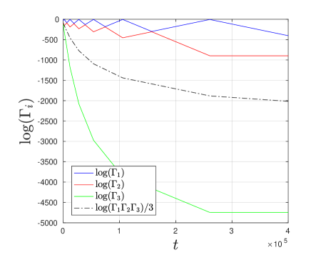
as functions of $t$ over some finite time interval $[t_{1},t_{2}]$. We restrict our attention to the so called tumbling case, that is, all $v_{i}$ are non-zero initially. This case might be considered as the most generic one in the context of the model under consideration. For convenience, we restrict ourselves in this work to the numerical solution which was already considered in Kiefer:2018uyv . The part of the solution plotted in Fig. 2(b) extends over one Kasner era. We regard this solution to occur at the transition into the asymptotic regime.

The numerical accuracy of our solution has been confirmed by checking the (approximate) preservation of the Hamiltonian constraint $\mathcal{H}=0$, and the constant of motion $C^{2}-1=0$. Both $\mathcal{H}$ and $C^{2}-1$ stay at order $10^{-15}$. We believe that the effect of chaos is negligible in a single Kasner era. For further details see Kiefer:2018uyv .

III Calculation of the Kretschmann scalar

We are interested in the temporal evolution of curvature invariants when approaching the singularity. Particular interest lies in the evolution of the Kretschmann scalar, which can be decomposed as

$$R_{\mu\nu\lambda\sigma}R^{\mu\nu\lambda\sigma}=C_{\mu\nu\lambda\sigma}C^{\mu\nu\lambda\sigma}+2R_{\mu\nu}R^{\mu\nu}-\frac{1}{3}R^{2}\ ,$$ (12)

where $C^{\mu}{}_{\nu\lambda\sigma}$ is the Weyl tensor, $R_{\mu\nu}$ is the Ricci tensor and $R$ the Ricci scalar. For our purposes it is convenient to make use of the constraints and the equations of motion to simplify the expressions such that they are suited for a numerical evaluation. We will do so throughout the calculation in this section and bring our expression into a form that is ready for a numerical evaluation. This means that all expressions should only involve the variables (11) as well as the constants $p_{T}^{\prime}\equiv 12p_{T}$ and $C$. Furthermore we shall use the quasi-Gaussian gauge $N^{i}=0$ while keeping the lapse $N$ unspecified. We now proceed by calculating the terms on the right-hand side of equation (12).

From the Einstein field equations $R_{\mu\nu}-\frac{1}{2}Rg_{\mu\nu}=\kappa T_{\mu\nu}=\kappa\rho u_{\mu}u_{\nu}$ it follows that we can write

$$R_{\mu\nu}R^{\mu\nu}=\kappa^{2}T_{\mu\nu}T^{\mu\nu}=\kappa^{2}\rho^{2}\quad\text{and}\quad R=-\kappa T^{\mu}{}_{\mu}=\kappa\rho\ .$$ (13)

Recall that in the model under consideration

$$\rho=\frac{p_{T}\textnormal{e}^{-3\alpha}}{\sqrt{1+h^{ij}u_{i}u_{j}}}=\frac{p_{T}}{\sqrt{\Gamma_{1}\Gamma_{2}\Gamma_{3}+C^{2}\left(\Gamma_{2}\Gamma_{3}v_{1}^{2}+\Gamma_{1}\Gamma_{3}v_{2}^{2}+\Gamma_{1}\Gamma_{2}v_{3}^{2}\right)}}\ .$$ (14)

We conclude that the Ricci part $2R_{\mu\nu}R^{\mu\nu}-\frac{1}{3}R^{2}$ of the Kretschmann scalar blows up as

$$\left[\Gamma_{1}\Gamma_{2}\Gamma_{3}+C^{2}\left(\Gamma_{2}\Gamma_{3}v_{1}^{2}+\Gamma_{1}\Gamma_{3}v_{2}^{2}+\Gamma_{1}\Gamma_{2}v_{3}^{2}\right)\right]^{-1}$$ (15)

when approaching the singularity. The calculation of the Weyl part of the Kretschmann scalar, however, is less trivial. The 3+1 split allows for a decomposition of the Weyl tensor into electric and magnetic part (see e.g. Alcubierre ) according to

$$C_{\mu\nu\lambda\sigma}C^{\mu\nu\lambda\sigma}=8\left(E_{ij}E^{ij}-B_{ij}B^{ij}\right)\quad\text{where}$$ (16)

$$E_{ij}=K_{ij}K_{k}{}^{k}-K_{i}{}^{k}K_{jk}+{}^{(3)}R_{ij}-\frac{\kappa}{2}\left[S_{ij}+\frac{1}{3}h_{ij}\left(4\epsilon-S^{i}{}_{i}\right)\right]\ ,$$

$$B_{ij}=\epsilon_{ikl}\left[D^{k}K_{j}{}^{l}-\frac{\kappa}{2}\delta^{k}_{j}j^{l}\right]\ ,$$

with $\epsilon_{ikl}$ being the Levi-Civita tensor. The other objects involved in the decomposition are explained below. Now let $P^{\mu}_{\nu}=\delta^{\mu}_{\nu}+n^{\mu}n_{\nu}$ denote the projector onto spatial hypersurfaces orthogonal to the normal vector $\{n^{\mu}\}=(1/N,0,0,0)$, that is $P^{\mu}_{i}=\delta^{\mu}_{i}$, $P^{\mu}_{0}=0$. $D_{i}$ denotes the 3 dimensional covariant derivative on these hypersurfaces. The quantities involved in equation (16) are

$$\begin{gathered}\epsilon=n^{\mu}n^{\nu}T_{\mu\nu}=\rho(1+u^{i}u_{i})\ ,\\ S_{ij}=P^{\mu}_{i}P^{\nu}_{j}T_{\mu\nu}=\rho u_{i}u_{j}\ ,\\ j^{i}=-P^{i\mu}n^{\nu}T_{\mu\nu}=p_{T}u^{i}/\sqrt{h}\ ,\end{gathered}$$ (17)

where $\epsilon$, $S_{ij}$ and $j^{i}$ are the energy density, the shear density and the momentum density as measured by Eulerian observers (observers with four velocity $n^{\mu}$).

A direct calculation yields

$$4N^{2}\Gamma_{1}\Gamma_{2}\Gamma_{3}B_{ij}B^{ij} =\left(\Gamma_{1}^{2}+\Gamma_{2}^{2}+\Gamma_{3}^{2}\right)\left[\frac{\dot{\Gamma}_{1}}{\Gamma_{1}}+\frac{\dot{\Gamma}_{2}}{\Gamma_{2}}+\frac{\dot{\Gamma}_{3}}{\Gamma_{3}}\right]^{2}$$ (18)

$$+\left(\Gamma_{1}+\Gamma_{2}+\Gamma_{3}\right)\left(\dot{\Gamma}_{1}+\dot{\Gamma}_{2}+\dot{\Gamma}_{3}\right)\left(\frac{\dot{\Gamma}_{1}}{\Gamma_{1}}+\frac{\dot{\Gamma}_{2}}{\Gamma_{2}}+\frac{\dot{\Gamma}_{3}}{\Gamma_{3}}\right)$$

$$+\frac{1}{4}\left(\Gamma_{1}+\Gamma_{2}+\Gamma_{3}\right)^{2}\left[\frac{\dot{\Gamma}_{1}^{2}}{\Gamma_{1}^{2}}+\frac{\dot{\Gamma}_{2}^{2}}{\Gamma_{2}^{2}}+\frac{\dot{\Gamma}_{3}^{2}}{\Gamma_{3}^{2}}-3\left(\frac{\dot{\Gamma}_{1}}{\Gamma_{1}}+\frac{\dot{\Gamma}_{2}}{\Gamma_{2}}+\frac{\dot{\Gamma}_{3}}{\Gamma_{3}}\right)^{2}\right]$$

$$+\frac{N^{2}C^{2}p_{T}^{\prime 2}\left(\Gamma_{1}+\Gamma_{2}+\Gamma_{3}\right)^{2}}{24\Gamma_{1}\Gamma_{2}\Gamma_{3}}\left[\frac{v_{1}^{2}}{I_{1}}+\frac{v_{2}^{2}}{I_{2}}+\frac{v_{3}^{2}}{I_{3}}\right]\ .$$

Let us now turn to the computation of $E_{ij}E^{ij}$, which can be written out as

$$E_{ij}E^{ij}= K^{i}{}_{j}K^{j}{}_{k}\left(K^{k}{}_{l}K^{l}{}_{i}-2K^{k}{}_{i}K^{l}{}_{l}\right)+K^{i}{}_{j}K^{j}{}_{i}(K^{l}{}_{l})^{2}$$ (19)

$$-2\left(K^{i}{}_{l}K^{lj}-K^{l}{}_{l}K^{ij}\right)\ {}^{(3)}R_{ij}+\ {}^{(3)}R_{ij}{}^{(3)}R^{ij}$$

$$+6\rho\left(K^{i}{}_{l}K^{lj}-K^{l}{}_{l}K^{ij}-{}^{(3)}R^{ij}\right)u_{i}u_{j}$$

$$+\rho\left(8+6u_{k}u^{k}\right)\left[K^{i}{}_{j}K^{j}{}_{i}-(K^{l}{}_{l})^{2}-{}^{(3)}R\right]$$

$$+\rho^{2}\left[54\left(u_{k}u^{k}\right)^{2}+96\ u_{k}u^{k}+48\right]\ .$$

We now evaluate the single terms. The term in the first line of (19) right after the equal sign can be written as

$$8N^{4}\left[K^{i}{}_{j}K^{j}{}_{k}\left(K^{k}{}_{l}K^{l}{}_{i}-2K^{k}{}_{i}K^{l}{}_{l}\right)+K^{i}{}_{j}K^{j}{}_{i}(K^{l}{}_{l})^{2}\right]=$$ (20)

$$\left[(\log\Gamma_{1})^{\cdot}(\log\Gamma_{2})^{\cdot}\right]^{2}+\left[(\log\Gamma_{1})^{\cdot}(\log\Gamma_{3})^{\cdot}\right]^{2}+\left[(\log\Gamma_{2})^{\cdot}(\log\Gamma_{3})^{\cdot}\right]^{2}$$

$$+(\log\Gamma_{1})^{\cdot}(\log\Gamma_{2})^{\cdot}(\log\Gamma_{3})^{\cdot}\left[(\log\Gamma_{1})^{\cdot}+(\log\Gamma_{2})^{\cdot}+(\log\Gamma_{3})^{\cdot}\right]$$

$$+N^{4}C^{4}p_{T}^{\prime\ 4}\left[\frac{v_{1}^{4}}{\Gamma_{1}^{2}(\Gamma_{2}-\Gamma_{3})^{4}}+\frac{v_{2}^{4}}{\Gamma_{2}^{2}(\Gamma_{1}-\Gamma_{3})^{4}}+\frac{v_{3}^{4}}{\Gamma_{3}^{2}(\Gamma_{1}-\Gamma_{2})^{4}}\right.$$

$$\left.+\frac{2v_{1}^{2}v_{2}^{2}}{\Gamma_{1}\Gamma_{2}\left(\Gamma_{1}-\Gamma_{3}\right)^{2}\left(\Gamma_{2}-\Gamma_{3}\right)^{2}}\right.$$

$$\left.+\frac{2v_{2}^{2}v_{3}^{2}}{\Gamma_{3}\Gamma_{2}\left(\Gamma_{2}-\Gamma_{1}\right)^{2}\left(\Gamma_{3}-\Gamma_{1}\right)^{2}}+\frac{2v_{1}^{2}v_{3}^{2}}{\Gamma_{1}\Gamma_{3}\left(\Gamma_{1}-\Gamma_{2}\right)^{2}\left(\Gamma_{3}-\Gamma_{2}\right)^{2}}\right]$$

$$-\frac{N^{2}C^{2}p_{T}^{\prime\ 2}v_{1}^{2}}{\Gamma_{1}(\Gamma_{2}-\Gamma_{3})^{2}}\left[(\log\Gamma_{1})^{\cdot}\left[(\log\Gamma_{2})^{\cdot}+(\log\Gamma_{3})^{\cdot}-(\log\Gamma_{1})^{\cdot}\right]+2(\log\Gamma_{2})^{\cdot}(\log\Gamma_{3})^{\cdot}\right]$$

$$-\frac{N^{2}C^{2}p_{T}^{\prime\ 2}v_{2}^{2}}{\Gamma_{2}(\Gamma_{1}-\Gamma_{3})^{2}}\left[(\log\Gamma_{2})^{\cdot}\left[(\log\Gamma_{1})^{\cdot}+(\log\Gamma_{3})^{\cdot}-(\log\Gamma_{2})^{\cdot}\right]+2(\log\Gamma_{1})^{\cdot}(\log\Gamma_{3})^{\cdot}\right]$$

$$-\frac{N^{2}C^{2}p_{T}^{\prime\ 2}v_{3}^{2}}{\Gamma_{3}(\Gamma_{2}-\Gamma_{1})^{2}}\left[(\log\Gamma_{3})^{\cdot}\left[(\log\Gamma_{2})^{\cdot}+(\log\Gamma_{1})^{\cdot}-(\log\Gamma_{3})^{\cdot}\right]+2(\log\Gamma_{2})^{\cdot}(\log\Gamma_{1})^{\cdot}\right]\ .$$

We denote the three-dimensional Ricci tensor of the diagonal model by ${}^{(3)}\bar{R}_{ij}$. The three-dimensional Ricci tensor of the non-diagonal model can then obtained via rotation according to ${}^{(3)}R_{ij}=O_{i}{}^{k}O_{j}{}^{l}\ {}^{(3)}\bar{R}_{kl}$. The only non-vanishing components of ${}^{(3)}\bar{R}_{ij}$ are given by

$${}^{(3)}\bar{R}_{11} =1+\frac{\Gamma_{1}^{2}}{2\Gamma_{2}\Gamma_{3}}-\frac{\Gamma_{2}}{2\Gamma_{3}}-\frac{\Gamma_{3}}{2\Gamma_{2}}$$ (21)

$${}^{(3)}\bar{R}_{22} =1+\frac{\Gamma_{2}^{2}}{2\Gamma_{1}\Gamma_{3}}-\frac{\Gamma_{1}}{2\Gamma_{3}}-\frac{\Gamma_{3}}{2\Gamma_{1}}$$

$${}^{(3)}\bar{R}_{33} =1+\frac{\Gamma_{3}^{2}}{2\Gamma_{1}\Gamma_{2}}-\frac{\Gamma_{1}}{2\Gamma_{2}}-\frac{\Gamma_{2}}{2\Gamma_{1}}\ .$$

The first term in the second line of (19) reads

$$-2\left(K^{i}{}_{l}K^{lj}-K^{l}{}_{l}K^{ij}\right)\ {}^{(3)}R_{ij}=\frac{\left(\Gamma_{2}+\Gamma_{3}-\Gamma_{1}\right)(\log\Gamma_{2})^{\cdot}(\log\Gamma_{3})^{\cdot}}{2N^{2}\Gamma_{2}\Gamma_{3}}$$ (22)

$$\quad+\frac{\left(\Gamma_{1}+\Gamma_{3}-\Gamma_{2}\right)(\log\Gamma_{1})^{\cdot}(\log\Gamma_{3})^{\cdot}}{2N^{2}\Gamma_{1}\Gamma_{3}}+\frac{\left(\Gamma_{1}+\Gamma_{2}-\Gamma_{3}\right)(\log\Gamma_{1})^{\cdot}(\log\Gamma_{2})^{\cdot}}{2N^{2}\Gamma_{2}\Gamma_{1}}$$

$$\quad+\frac{C^{2}p_{T}^{\prime\ 2}}{2\Gamma_{1}\Gamma_{2}\Gamma_{3}}\left[\frac{\left(\Gamma_{1}-\Gamma_{2}-\Gamma_{3}\right)v_{1}^{\ 2}}{\left(\Gamma_{2}-\Gamma_{3}\right)^{2}}+\frac{\left(\Gamma_{2}-\Gamma_{1}-\Gamma_{3}\right)v_{2}^{\ 2}}{\left(\Gamma_{1}-\Gamma_{3}\right)^{2}}+\frac{\left(\Gamma_{3}-\Gamma_{1}-\Gamma_{2}\right)v_{3}^{\ 2}}{\left(\Gamma_{1}-\Gamma_{2}\right)^{2}}\right]\ .$$

The three-dimensional Ricci squared scalar can be written as

$${}^{(3)}R_{ij}{}^{(3)}R^{ij}=\frac{\left(\Gamma_{1}^{2}-12I_{1}\Gamma_{2}\Gamma_{3}\right)^{2}+\left(\Gamma_{2}^{2}-12I_{2}\Gamma_{1}\Gamma_{3}\right)^{2}+\left(\Gamma_{3}^{2}-12I_{3}\Gamma_{1}\Gamma_{2}\right)^{2}}{4\left(\Gamma_{1}\Gamma_{2}\Gamma_{3}\right)^{2}}\ .$$ (23)

The term in the third line of (19) becomes

$$6\rho\left(K^{i}{}_{l}K^{lj}-K^{l}{}_{l}K^{ij}-{}^{(3)}R^{ij}\right)u_{i}u_{j}=$$ (24)

$$\frac{3\rho C^{3}p_{T}^{\prime}v_{1}v_{2}v_{3}}{N\sqrt{\Gamma_{1}\Gamma_{2}\Gamma_{3}}}\left[\frac{(\log\Gamma_{1})^{\cdot}}{\Gamma_{3}-\Gamma_{2}}+\frac{(\log\Gamma_{2})^{\cdot}}{\Gamma_{1}-\Gamma_{3}}+\frac{(\log\Gamma_{3})^{\cdot}}{\Gamma_{2}-\Gamma_{1}}\right]$$

$$+\frac{3\rho C^{4}p_{T}^{\prime\ 2}}{2}\left[\frac{(\Gamma_{2}-\Gamma_{3})^{2}v_{2}v_{3}}{\Gamma_{2}\Gamma_{3}(\Gamma_{1}-\Gamma_{2})^{2}(\Gamma_{1}-\Gamma_{3})^{2}}\right.$$

$$+\left.\frac{(\Gamma_{1}-\Gamma_{3})^{2}v_{1}v_{3}}{\Gamma_{1}\Gamma_{3}(\Gamma_{2}-\Gamma_{3})^{2}(\Gamma_{2}-\Gamma_{1})^{2}}+\frac{(\Gamma_{1}-\Gamma_{2})^{2}v_{1}v_{2}}{\Gamma_{1}\Gamma_{2}(\Gamma_{3}-\Gamma_{1})^{2}(\Gamma_{3}-\Gamma_{2})^{2}}\right]$$

$$+\frac{3\rho C^{2}}{\Gamma_{1}\Gamma_{2}\Gamma_{3}}\left[\left((\Gamma_{2}-\Gamma_{3})^{2}-\Gamma_{1}^{2}-\frac{\Gamma_{1}\Gamma_{2}\Gamma_{3}}{2N^{2}}(\log\Gamma_{1})^{\cdot}\left[(\log\Gamma_{2})^{\cdot}+(\log\Gamma_{3})^{\cdot}\right]\right)\frac{v_{1}^{2}}{\Gamma_{1}}\right.$$

$$\left.+\left((\Gamma_{1}-\Gamma_{3})^{2}-\Gamma_{2}^{2}-\frac{\Gamma_{1}\Gamma_{2}\Gamma_{3}}{2N^{2}}(\log\Gamma_{2})^{\cdot}\left[(\log\Gamma_{1})^{\cdot}+(\log\Gamma_{3})^{\cdot}\right]\right)\frac{v_{2}^{2}}{\Gamma_{2}}\right.$$

$$\left.+\left((\Gamma_{1}-\Gamma_{2})^{2}-\Gamma_{3}^{2}-\frac{\Gamma_{1}\Gamma_{2}\Gamma_{3}}{2N^{2}}(\log\Gamma_{3})^{\cdot}\left[(\log\Gamma_{1})^{\cdot}+(\log\Gamma_{2})^{\cdot}\right]\right)\frac{v_{3}^{2}}{\Gamma_{3}}\right]$$

We can use the Hamiltonian constraint to simplify

$$K^{i}{}_{j}K^{j}{}_{i}-(K^{l}{}_{l})^{2}-{}^{(3)}R=-p_{T}^{\prime}\sqrt{\frac{1+u_{i}u^{i}}{\Gamma_{1}\Gamma_{2}\Gamma_{3}}}\ .$$ (25)

We therefore obtain a simple expression for the term in the fourth line of (19). Since we have direct numerical access to the quantities in the fourth and fifth line of (19), we will not manipulate them further.

It is well known that the Weyl squared scalar vanishes for the Friedmann models. The dust filled closed Friedmann universe is included in the model under consideration as the particular case for which $\Gamma_{1}=\Gamma_{2}=\Gamma_{3}$ and $C=0$. As a consistency check of our calculation we convinced ourselves that the Weyl squared scalar vanishes for these restrictions. We find that $B_{ij}B^{ij}$ and $E_{ij}E^{ij}$ vanish separately and hence $C_{\mu\nu\lambda\sigma}C^{\mu\nu\lambda\sigma}=0$ as expected.

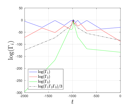
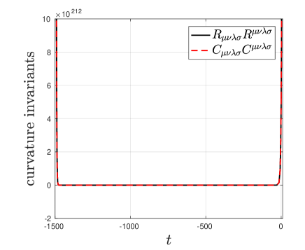
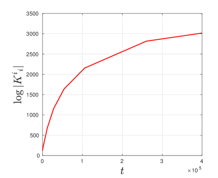
A numerical evaluation “close” to the point of recollapse is shown in Fig. 1. We note that the bare Kretschmann scalar appears to roughly blow up exponentially in $t$ and it rapidly exceeds the range of numbers that are accessible in Matlab. This is why from now on we turn to numerically evaluating the so-called Hubble normalized Kretschmann scalar $R_{\mu\nu\lambda\sigma}R^{\mu\nu\lambda\sigma}/|K^{i}{}_{i}|$. This quantity has the virtue of being dimensionless and numerically well behaved. The expansion scalar is given by

$$K^{i}{}_{i}=\frac{1}{2N}\left[(\log\Gamma_{1})^{\cdot}+(\log\Gamma_{2})^{\cdot}+(\log\Gamma_{3})^{\cdot}\right]=\frac{3}{N}\dot{\alpha}\ .$$ (26)

(a) Plot of $\Gamma_{i}$ variables “close” to the recollapse.

(b) Plot of Kretschmann and Weyl squared scalar corresponding to FIG. 1(a).

Figure 1: Plot (a) shows the result of the application of the shooting method described in Kiefer:2018uyv “close” to the recollapse (which is roughly at $t\approx-1000$). The plot (b) was obtained from a numerical calculation based on the result of section III.

IV The asymptotic regime close to the singularity

We remark again that we are considering the tumbling case. We expect, however, that a similar discussion also holds for the non-tumbling and non-rotating cases.

In order to simplify the dynamics of Bianchi IX (see, e.g. the review in bkl ) we make two assumptions. The first assumption states that the anisotropy of space grows without bound. This means that the solution enters the regime

$$\Gamma_{1}\gg\Gamma_{2}\gg\Gamma_{3}\ ,$$ (27)

where the ordering of indices depends on the initial conditions and is mostly irrelevant for our discussion. The second assumption states that the Euler angles assume constant values:

$$(\theta,\phi,\psi)\rightarrow(\theta_{0},\phi_{0},\psi_{0})\ ,$$ (28)

that is, the rotation of the principal axes stops for all practical purposes and the metric becomes effectively diagonal. For our variables this means that the dust velocities $v_{i}$ assume constant values. The main purpose of the article Kiefer:2018uyv was to provide a numerical verification for the two assumptions.

According to the phrase “matter does not matter” we expect the matter terms in the Kretschmann scalar to be negligible in the asymptotic regime, that is, the Weyl part should dominate over the Ricci part.

During Kasner epochs (i.e. between two successive bounces in the asymptotic regime) we expect the most relevant term to be the term in the first two lines of (20) right after the equality-sign. We therefore assume now that the Kretschmann scalar can be approximated by

$$R_{\mu\nu\lambda\sigma}R^{\mu\nu\lambda\sigma}\approx\frac{1}{N^{4}} \left(\left[(\log\Gamma_{1})^{\cdot}(\log\Gamma_{2})^{\cdot}\right]^{2}+\left[(\log\Gamma_{1})^{\cdot}(\log\Gamma_{3})^{\cdot}\right]^{2}+\left[(\log\Gamma_{2})^{\cdot}(\log\Gamma_{3})^{\cdot}\right]^{2}\right.$$ (29)

$$\left.\ +(\log\Gamma_{1})^{\cdot}(\log\Gamma_{2})^{\cdot}(\log\Gamma_{3})^{\cdot}\left[(\log\Gamma_{1})^{\cdot}+(\log\Gamma_{2})^{\cdot}+(\log\Gamma_{3})^{\cdot}\right]\right)\ .$$

This claim is confirmed by our numerical simulations. We remark that this term corresponds exactly to the Weyl squared scalar of the Bianchi I model with the metric

$$\textnormal{d}s^{2}=-N^{2}\textnormal{d}t^{2}+\Gamma_{1}\textnormal{d}x^{2}+\Gamma_{2}\textnormal{d}y^{2}+\Gamma_{1}\textnormal{d}z^{2}\ .$$ (30)

The Weyl tensor of the Bianchi I model has only an electric part, and the magnetic part vanishes (in the quasi-Gaussian gauge).

During Kasner epochs the time evolution can be parameterized using the Lifshitz -Khalatnikov parameter $u$ following the considerations in bkl . Doing so and using the assumption (29) we obtain that the Hubble-normalized Kretschmann scalar can be approximated by

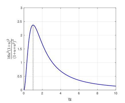
$$R_{\mu\nu\lambda\sigma}R^{\mu\nu\lambda\sigma}/|K^{i}{}_{i}|^{4}\approx\frac{16u^{2}(1+u)^{2}}{\left(1+u+u^{2}\right)^{3}}\qquad\text{during Kasner epochs}.$$ (31)

Consequently the Kretschmann scalar blows up like the expansion $K^{i}{}_{i}$ to the power $4$ during Kasner eras. In order to understand the temporal evolution of the Kretschmann scalar over the course of one epoch we have plotted the expression on the right hand side of (31) as a function of $u$ in Fig. 2(a). It is important that the function has a maximum in $u=1$.

The BKL refers to bounces from the curvature potential as transformations of the first kind while they call bounces from centrifugal walls transformations of the second kind. Transformations of the first kind change the Lifshitz-Khalatnikov parameter according to $u\overset{1}{\rightarrow}u-1$. Transformations of the second kind interchange the values of the velocities according to $(\log\Gamma_{1})^{\cdot}\overset{2}{\rightarrow}(\log\Gamma_{2})^{\cdot}$, $(\log\Gamma_{2})^{\cdot}\overset{2}{\rightarrow}(\log\Gamma_{1})^{\cdot}$ and leave the value of $u$ unchanged, i.e. $u\overset{2}{\rightarrow}u$. It follows that $\overset{1}{\rightarrow}$ changes the value of the Hubble normalized Kretschmann scalar (31) while $\overset{2}{\rightarrow}$ does not. According to the analysis in bkl a typical Kasner era can be expressed as a sequence of $n$ Kasner epochs which starts with an epoch that has a maximum $u$-value larger than $1$ when evolving towards the singularity. The value of $u$ decreases with each transformation of the first kind and ends with the epoch for which $u$ becomes smaller than $1$ for the first time, e.g.

$$1<u_{1}=u_{\text{max}}\overset{1}{\rightarrow}u_{2}\overset{2}{\rightarrow}u_{3}\overset{1}{\rightarrow}u_{4}\overset{2}{\rightarrow}u_{5}\overset{1}{\rightarrow}\ \ldots\ \overset{2}{\rightarrow}u_{n-1}\overset{1}{\rightarrow}u_{n}=u_{\text{min}}<1\ .$$ (32)

It should be remarked at this point that the $u$-map was found to be asymptotically exact for particular cases (for a collection of rigorous results concerning the $u$-map see Uggla ). A solution of the discrete mixmaster map and a detailed study of its chaotic nature for the vacuum Bianchi IX case can be found in Chernoff_Barrow_1972 .

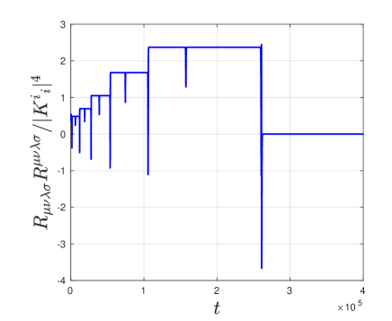
We are now in the position to provide a picture of the behaviour of the Kretschmann scalar over the course of one Kasner era: According to the formula (31) plotted in Fig. 2(a) and (32) we expect the Hubble normalized Kretschmann scalar to increase its value with each transformation of the first kind before it hits the value $u_{\text{min}}<1$ for which it decreases again. This is apart from the behaviour in the vicinity of the bounces precisely what we observe in the numerically evaluated Hubble normalized scalar plotted in Fig. 2. We remark that we regard the part of the solution plotted in Fig. 2(b) to be not quite in the asymptotic regime but rather at the tansition into the asymptotic regime.

(a) Plot of the function $\frac{16u^{2}(1+u)^{2}}{\left(1+u+u^{2}\right)^{3}}$ on the right hand side of (31).

(b) Plot of the variables $\log(\Gamma_{i})$ obtained via the shooting method.

(c) Plot of the logarithm of the expansion.

(d) Plot of the Hubble normalized Kretschmann scalar.

Figure 2: The plot (b) was obtained by the shooting method described in Kiefer:2018uyv . One can see a typical Kasner era composed of epochs that are approximately connected by transformations of the first and second kind. The output of the shooting method was used to obtain the plots (c) and (d) based on the calculation in section III of this paper.

It was helpful, in this paper, to support the computations by using the tensor algebra package xAct xAct . Numerical calculations were performed using MATLAB R2016b.

V Summary

The main purpose of this paper is to provide a description of the temporal behaviour of the Kretschmann scalar in the asymptotic regime. In this regime the volume density, being proportional to the product of the three directional scale factors, evolves towards zero bkl , but this is not a satisfactory indication of the singularity as it depends on the choice of coordinates. The blowing up of curvature invariants, on the other hand, shows that we are dealing with a genuine curvature singularity.

During Kasner epochs, $R_{\mu\nu\lambda\sigma}R^{\mu\nu\lambda\sigma}$ increases like the expansion to the power four. Over the course of a single Kasner era the value of the Hubble normalized Kretschmann scalar increases until it drops down to a finite value when it ends. This process will repeat itself with the beginning of the next Kasner era until the system approaches the singularity.

The present paper is supposed to be an extension of our previous paper Kiefer:2018uyv , which considers, for simplicity, only the tilted dust field as a source. The discussion of other tilted fluids goes beyond the scope of our present programme. The effect of tilted radiation, which has been studied analytically and numerically in the recent paper Ganguly:2017qff , is particularly interesting.

The asymptotic regimes of the Bianchi IX and BVIII models are quite similar VBiel . Both models have been used to derive the BKL scenario BKL22 .

The asymptotic regime approximates well the dynamics near the singularity. This is why it was recently used in the struggle for removing the singularity of the BKL scenario by quantization AWG .

References

• (1) C. Kiefer, N. Kwidzinski and W. Piechocki, “On the dynamics of the general Bianchi IX spacetime near the singularity,” Eur. Phys. J. C 78 (2018) 691.
• (2) S.W. Hawking and G.F.R. Ellis, The Large Scale Structure of Space-Time (Cambridge University Press, Cambridge, 1973).
• (3) S. Hawking and R. Penrose, The Nature of Space and Time (Princeton University Press, Princeton, 1996).
• (4) J. M. M. Senovilla, “Singularity Theorems and Their Consequences”, Gen. Rel. Grav. 30, 701 (1998).
• (5) C. Uggla, “Spacetime singularities: recent developments”, Int. J. Mod. Phys. D 22, 1330002 (2013).
• (6) V. Belinski and M. Henneaux, The Cosmological Singularity (Cambridge University Press, Cambridge, 2017).
• (7) H. Ringström, “Curvature blow up in Bianchi VIII and IX vacuum spacetimes”, Class. Quant. Grav. 17, 713 (2000).
• (8) J. D. Barrow and S. Hervik , “The Weyl tensor in spatially homogeneous cosmological models”, Class. Quant. Grav. 19, 155 (2002).
• (9) R. Penrose, Singularities and Time-Asymmetry”. In S. W. Hawking; W. Israel. General Relativity: An Einstein Centenary Survey. Cambridge University Press. pp. 581–638. (1979)
• (10) E. Czuchry, N. Kwidzinski and W. Piechocki, “Comparing the dynamics of diagonal and general Bianchi IX spacetime”, Eur. Phys. J. C, accepted for publication.
• (11) A. R. King and G. F. R. Ellis, “Tilted homogeneous cosmological models”, Commun. Math. Phys. 31, 209 (1973).
• (12) R. A. Matzner, L. C. Shepley and J. B. Warren, “Dynamics of SO(3,R)-Homogeneous Cosmologies”, Ann. Phys. (N.Y.) 57, 401 (1970).
• (13) L. P. Grishchuk, A. G. Doroshkevich and V. N. Lukash, “The model of mixmaster universe with arbitrarily moving matter”, J. Exp. Theor. Phys. 34, 1 (1972).
• (14) M. P. Ryan, “Qualitative cosmology: diagrammatic solutions for Bianchi type IX universes with expansion, rotation, and shear. I. The symmetric case”, Ann. Phys. (N.Y.) 65, 506 (1971).
• (15) M. P. Ryan, “Qualitative cosmology: diagrammatic solutions for Bianchi type IX universes with expansion, rotation, and shear. II. The general case”, Ann. Phys. (N.Y.) 68, 541 (1971).
• (16) R. T. Jantzen, “Spatially homogeneous dynamics: a unified picture”, arXiv:gr-qc/0102035. Originally published in the Proceedings of the International School Enrico Fermi, Course LXXXVI (1982) on Gamov Cosmology, edited by R. Ruffini and F. Melchiorri (North Holland, Amsterdam, 1987), pp. 61–147.
• (17) M. P. Ryan, Hamiltonian Cosmology (Springer, Berlin, 1972).
• (18) M. P. Ryan and L. C. Shepley, Homogeneous Relativistic Cosmologies (Princeton University Press, Princeton, 1975).
• (19) V. A. Belinskii, I. M. Khalatnikov, and M. P. Ryan, “The oscillatory regime near the singularity in Bianchi-type IX universes”, Preprint 469 (1971), Landau Institute for Theoretical Physics, Moscow (unpublished); published as sections 1 and 2 in M. P. Ryan, Ann. Phys. (N.Y.) 70, 301 (1971).
• (20) M. Alcubierre, Introduction to 3+1 Numerical Relativity (Oxford University Press, Oxford, 2008).
• (21) X. Lin and R. M. Wald, “Proof of the closed-universe recollapse conjecture for general bianchi type-IX cosmologies”, Phys. Rev. D 44, 2444 (1990).
• (22) L. P. Chernoff and V. N. Barrow, “The model of mixmaster universe with arbitrarily moving matter”, J. Exp. Theor. Phys. 34, 1 (1972).
• (23) J. M. Martín-García, “xAct: Efficient tensor computer algebra for the Wolfram language”, http://www.xact.es.
• (24) C. Ganguly and J. D. Barrow, “Evolution of cyclic mixmaster universes with noncomoving radiation,” Phys. Rev. D 96, 123534 (2017).
• (25) V. A. Belinski, private communication.
• (26) V. A. Belinskii, I. M. Khalatnikov, and E. M. Lifshitz, “Oscillatory approach to a singular point in the relativistic cosmology”, Adv. Phys. 19, 525 (1970).
• (27) A. Góźdź, W. Piechocki and G. Plewa, “Quantum Belinski-Khalatnikov-Lifshitz scenario”, Eur. Phys. J. C 79 (2019) 45.