New ECCM Techniques Against Noise-like and/or Coherent Interferers

Abstract

Multiple-stage adaptive architectures are conceived to face with the problem of target detection buried in noise, clutter, and intentional interference. First, a scenario where the radar system is under the electronic attack of noise-like interferers is considered. In this context, two sets of training samples are jointly exploited to devise a novel two-step estimation procedure of the interference covariance matrix. Then, this estimate is plugged in the adaptive matched filter to mitigate the deleterious effects of the noise-like jammers on radar sensitivity. Besides, a second scenario, which extends the former by including the presence of coherent jammers, is addressed. Specifically, the sparse nature of data is brought to light and the compressive sensing paradigm is applied to estimate target response and coherent jammers amplitudes. The likelihood ratio test, where the unknown parameters are replaced by previous estimates, is designed and assessed. Remarkably, the sparse approach allows for echo classification and estimation of both angles of arrival and number of the interfering sources. The performance analysis, conducted resorting to simulated data, highlights the effectiveness of the newly proposed architectures also in comparison with suitable competing architectures (when they exist).

I Introduction

In the last decades, radar art has been significantly influenced by the advances in technology as corroborated by the last-generation processing boards capable of performing huge amounts of computations in a very short time while keeping the costs relatively low. This abundance of computation power has allowed for the development of radar systems endowed with more and more sophisticated processing schemes.

To provide a tangible example, let us focus on search radars which are primarily concerned with the detection and tracking of targets embedded in thermal noise, clutter, and, possibly, intentional interference, also known as Electronic Countermeasure (ECM) [1, 2, 3, 4]. In this context, the open literature is rich with novel contributions on adaptive detection with the result that detection architectures are evolving towards a continuous performance enhancement. Consider, for example, the space-time detection algorithms that exploit large volumes of data from sensor arrays and/or pulse trains to take advantage of temporal and spatial integration/diversity [5, 6, 7, 8, 9, 10, 11, 12, 13, 14, 15]. Another route followed by the radar community to improve the detection performance consists in using the available information about the structure of the Interference Covariance Matrix (ICM) at the design stage. As a matter of fact, special structures of the ICM are induced by the system and/or interference properties [16, 17, 18, 19, 20, 21, 22, 23, 24, 25, 26]. As an illustration of this fact, consider those decision rules devised assuming that the ICM is centrohermitian. These algorithms allow us to reduce the number of training samples required for the ICM estimation [27, 16, 17, 28, 18, 19, 20, 21, 22, 23] by almost a half while maintaining a satisfactory detection performance. Further examples are provided in [24, 25], where it is shown that the spectral symmetry of the clutter can be used for instance to obtain gains of about $3$ dB (in SINR, namely Signal-to-Interference plus Noise Ratio), for a Probability of Detection $P_{d}=0.9$ and Probability of False Alarm $P_{fa}=10^{-4}$, in comparison to conventional detectors.

In most of the above contributions, the ICM results from the superposition of two components representative of the following two interference sources

• the electronic devices generating thermal noise, which is ubiquitous;

• the specific operating environment, whose backscattering gives rise to the clutter component, which is assumed dominant with respect to thermal noise.

Additionally, conventional ICM estimation procedures exploit training samples (secondary data) collected in the proximity of the Cell Under Test (CUT).

However, radars might be potential targets of electronic attacks by an adversary force, which can use, for instance, active techniques aimed at protecting a platform from being detected and tracked by the radar [4]. This is accomplished through two approaches: masking and deception. Noncoherent Jammers or Noise-Like Jammers (NLJs) attempt to mask targets generating nondeceptive interference which blends into the thermal noise of the radar receiver. As a consequence, the radar sensitivity is degraded due to the increase of the constant false alarm rate threshold which adapts to the higher level of noise [2, 4]. In addition, this increase makes more difficult to discover that jamming is taking place [3, 29].

On the other hand, the Coherent Jammers (CJs) transmit low-duty cycle signals intended to inject false information into the radar processor. Specifically, they are capable of receiving, modifying, amplifying, and retransmitting the radar’s own signal to create false targets maintaining radar’s range, Doppler, and angle far away from the true position of the platform under protection [29, 30, 2, 4].

Against the aforementioned electronic attacks, radar designers have developed defense strategies referred to as Electronic Counter-CounterMeasure (ECCM) which can be categorized as antenna-related, transmitter-related, receiver-related, and signal-processing-related depending on the main radar subsystem where they take place [29]. The first line of defense against jamming is represented by the radar antenna, whose beampattern can be suitably exploited and/or shaped to eliminate sidelobe false targets or to attenuate the power of NLJs entering from the antenna sidelobes. The Sidelobe Blanker (SLB) is an ECCM technique against pulsed interferences [31, 32, 33] which compares the detected signal amplitude from the main channel with that of an auxiliary channel. Specifically, when the auxiliary channel signal power is greater than that from the main channel, it is likely that the radar is under attack of a CJ from the sidelobes and, hence, the detection is blanked. In the presence of continuous or high duty cycle interferers, the SLB becomes ineffective since it would inhibit the detection of true targets for most of the time. In these situations, the Sidelobe Canceler (SLC) represents a viable ECCM against NLJs [2, 34, 35]. It places nulls in the sidelobes of the main receiver beam along the directions of arrival of the NLJs which are adaptively estimated using auxiliary channels. Both the SLB and SLC can be jointly used to face with NLJs and CJs contemporaneously impinging on the sidelobes of the victim radar [36]. Finally, it is important to mention that modern radars employ a digitally based approach to implement the SLC function. Specifically, digital samples from each channel of an electronically scanned array are weighted to adaptively shape the resulting beampattern. These techniques belong to the more general family of algorithms called Adaptive Digital Beamforming [4], which can be classified as signal-processing-related ECCM.

In this paper, we devise adaptive detection architectures with signal-processing-related ECCM capabilities against the attack of NLJs and/or CJs from the antenna sidelobes. At the design stage, we focus on two operating scenarios which differ for the presence of an unknown number of CJs. More precisely, in the first scenario, the target echoes compete against thermal noise, clutter, and NLJs whose number is unknown, whereas the second scenario extends the former by including prospective CJs. Note that the second scenario is more difficult than the first one, which represents the starting point for the derivations allowing to easily drive the reader towards the design of more complex systems. Both detection problems are formulated in terms of binary hypothesis tests and, following the lead of [37], two independent sets of secondary data are assumed available for estimation purposes.

The first set comes from the conventional radar reference window surrounding the CUT and shares the same ICM components as the CUT including the clutter component. The other training set can be acquired by observing that the clutter contribution is, in general, range-dependent and tied up to the transmitted waveform. Therefore, it is possible to acquire data free of clutter components and affected by the thermal noise and possible jamming signals only. For instance, for a system employing pulse-to-pulse frequency agility which transmits one pulse, clutter-free data can be collected before transmitting the pulse waveform by listening to the environment. Another example of practical interest concerns radar systems transmitting coherent pulse trains with a sufficiently high pulse repetition interval. In this case, data collected before transmitting the next pulse and at high ranges (or after the instrumental range), result free of clutter contribution. However, unlike [37], in this paper, we propose a novel two-step procedure to estimate the ICM components in a more effective way. Specifically, the thermal noise and NLJ components are estimated using the second data set (first step). The latter estimate replaces the corresponding ICM components of the conventional data set, which is used to estimate the remaining unknown ICM component, namely, the clutter component (second step). The number of NLJs impinging on the victim radar is unknown and, hence, is estimated resorting to either the so-called Model Order Selection (MOS) rules [38], which provide more reliable results than the Maximum Likelihood Approach (MLA) in the presence of nested hypotheses, or a heuristic ad hoc procedure based on the MLA. Observe that the last procedure can also be classified as a MOS rule but it does not rely on an information criterion as in [38]. More importantly, the herein proposed ICM estimation procedure requires a less restrictive constraint on the required volume of data with respect to that presented in [37] (a point better explained in Section III-A). Finally, the detection problem in the presence of NLJs is solved by applying the two-step Generalized Likelihood Ratio Test (GLRT) design procedure [6] where the ICM of the CUT is replaced by the new estimate. The final result consists in a multiple-stage architecture capable of taking advantage of the information carried by the additional training data set.

The other considered detection problem also includes the presence of multiple CJs in addition to NLJs, clutter, and thermal noise. Under this assumption, we reformulate the problem at hand in order to bring to light its sparse nature. As a consequence, compressive sensing reconstruction algorithms arise as natural choices to solve it. In the specific case, we exploit the Sparse Learning via Iterative Minimization (SLIM) [39], due to its trade off between low computational cost and reconstruction performance, to jointly estimate (under the alternative hypothesis) the unknown target and CJs responses. More precisely, we compute the Likelihood Ratio Test (LRT) where the ICM is replaced by the previously derived estimate, while target response and CJ amplitudes are estimated by the SLIM. The exploitation of SLIM (or, generally speaking, compressed sensing algorithms) is due to the fact that, as a byproduct, it allows for echo classification and estimation of both angles of arrival (AOA) and number of the interfering sources. In fact, if the LRT statistic is over the detection threshold, the following situations may occur:

• only CJs are present (target response is zero while CJ amplitudes are nonzero);

• only the target is present (target response is nonzero while CJ amplitudes are zero);

• simultaneous presence of the target and CJs (target response and CJ amplitudes are nonzero).

With these remarks in mind, we use the estimates provided by SLIM to build up a decision logic capable of discriminating among the above conditions which, evidently, form a multiple hypothesis test. Remarkably, this approach can be used in place of the conventional SLB since it recognizes possible CJs echoes which can be concurrent with target echoes without blanking the detection. Thus, the proposed detection architecture features SLB/SLC functionalities overcoming the limitations of the SLB.

The remainder of the paper is organized as follows. Section II is devoted to problem formulation and definition of quantities used in the next derivations while the design of the detection architectures and estimation procedures are contained in Section III. In Section IV, the behavior of the proposed architectures is investigated by means of numerical examples. Finally, concluding remarks and future research tracks are given in Section V. Some derivations are confined in the appendices.

Notation and List of Acronyms

The reader is referred to Table I for the list of the acronyms contained in this paper. Moreover, vectors and matrices are denoted by boldface lower-case and upper-case letters, respectively. Symbols $\det(\cdot)$ and $\mbox{\rm tr}\,(\cdot)$ denote the determinant and the trace of a square matrix, respectively. Symbols $I$ and $\mathrm{𝟎}$ represent the identity matrix and the null vector or matrix of suitable dimensions, respectively. The imaginary unit is denoted by $j$. Given a vector $a$, $\mbox{\boldmath\bf diag}\,(\mbox{\boldmath{$a$}})$ indicates the diagonal matrix whose $i$th diagonal element is the $i$th entry of $a$. For a finite set $A,\;|A|$ stands for its cardinality. As to the numerical sets, ${\mathds{R}}$ is the set of real numbers, ${\mathds{R}}^{N\times M}$ is the set of $(N\times M)$-dimensional real matrices (or vectors if $M=1$), ${\mathds{C}}$ is the set of complex numbers, and ${\mathds{C}}^{N\times M}$ is the set of $(N\times M)$-dimensional complex matrices (or vectors if $M=1$). The $(k,l)$-entry (or $l$-entry) of a generic matrix $A$ (or vector $a$) is denoted by $\mbox{\boldmath{$A$}}(k,l)$ (or $\mbox{\boldmath{$a$}}(l)$). We use $(\cdot)^{T}$ and $(\cdot)^{\dagger}$ to denote transpose and conjugate transpose, respectively. The Clutter-to-Noise Ratio and the Jammer-to-Noise Ratio are denoted by CNR and JNR, respectively. The conditional probability of an event $A$ given the even $B$ is represented as $P(A|B)$. Finally, we write $\mbox{\boldmath{$x$}}\sim\mbox{$\mathcal{C}$}\mbox{$\mathcal{N}$}_{N}(\mbox{\boldmath{$m$}},\mbox{\boldmath{$M$}})$ if $x$ is a complex circular $N$-dimensional normal vector with mean $m$ and positive definite covariance matrix $M$, whereas $\mbox{\boldmath{$X$}}=[\mbox{\boldmath{$x$}}_{1},\ldots,\mbox{\boldmath{$x$}}_{M}]\sim\mbox{$\mathcal{C}$}\mbox{$\mathcal{N}$}_{N,M}(\mbox{\boldmath{$m$}},\mbox{\boldmath{$M$}},\mbox{\boldmath{$I$}})$ if $\mbox{\boldmath{$x$}}_{i}\sim\mbox{$\mathcal{C}$}\mbox{$\mathcal{N}$}_{N}(\mbox{\boldmath{$m$}},\mbox{\boldmath{$M$}})$, $\forall i=1,\ldots,M$, and are statistically independent.

II Problem Formulation

Consider a radar system which exploits $N$ spatial (identical) channels to sense the surrounding environment. The incoming signal is conditioned by means of a baseband down-conversion and a filtering matched to the transmitted pulse waveform. Next, the output of the matched filter is suitably sampled and the samples are organized into $N$-dimensional complex vectors representing the range bins [1, 13].

In what follows, we denote the vector of the returns from the CUT by $\mbox{\boldmath{$z$}}\in{\mathds{C}}^{N\times 1}$, while the conventional training set, formed by collecting the returns from the range bins surrounding the CUT [1, 5], is stored in the matrix $\mbox{\boldmath{$Z$}}=[\mbox{\boldmath{$z$}}_{1},\ldots,\mbox{\boldmath{$z$}}_{K}]\in{\mathds{C}}^{N\times K}$. Finally, we assume also that the system acquires an additional set of training vectors (free of the clutter component and affected by thermal noise and possible NLJs) by listening to the environment (namely, operating in passive mode) [37]. This second set is denoted by $\mbox{\boldmath{$R$}}=[\mbox{\boldmath{$r$}}_{1},\ldots,\mbox{\boldmath{$r$}}_{M}]\in{\mathds{C}}^{N\times M}$.

As stated in Section I, in this paper we focus our attention on two detection problems representative of two scenarios where the latter subsumes the former as a special case. This choice is dictated by the need to make the derivations easy to be followed. In fact, the scenarios differ for the presence of CJs in the CUT. Specifically, the first problem, which is the same as in [37], can be formulated as

$$\left\{\begin{array}[]{l}\begin{aligned} &H_{1,0}:\left\{\begin{array}[]{l}\mbox{\boldmath{$z$}}=\alpha_{T}\mbox{\boldmath{$v$}}(\theta_{T})+\mbox{\boldmath{$n$}}\\ \mbox{\boldmath{$z$}}_{k}=\mbox{\boldmath{$n$}}_{k},\ \mbox{\boldmath{$r$}}_{m}=\mbox{\boldmath{$m$}}_{m},\quad k=1,\ldots,K,\ m=1,\ldots,M,\\ \end{array}\right.\\ &H_{0,0}:\left\{\begin{array}[]{l}\mbox{\boldmath{$z$}}=\mbox{\boldmath{$n$}}\\ \mbox{\boldmath{$z$}}_{k}=\mbox{\boldmath{$n$}}_{k},\ \mbox{\boldmath{$r$}}_{m}=\mbox{\boldmath{$m$}}_{m},\quad k=1,\ldots,K,\ m=1,\ldots,M,\\ \end{array}\right.\end{aligned}\end{array}\right.$$ (1)

where

• $n$, $\mbox{\boldmath{$n$}}_{1},\ldots,\mbox{\boldmath{$n$}}_{K}$, $\mbox{\boldmath{$m$}}_{1},\ldots,\mbox{\boldmath{$m$}}_{M}$ are statistically independent random vectors distributed as follows: $[\mbox{\boldmath{$n$}},\mbox{\boldmath{$n$}}_{1},\ldots,\mbox{\boldmath{$n$}}_{K}]\sim\mbox{$\mathcal{C}$}\mbox{$\mathcal{N}$}_{N,K}({\mbox{\boldmath$0$}},\mbox{\boldmath{$M$}}_{1},\mbox{\boldmath{$I$}})$ and $[\mbox{\boldmath{$m$}}_{1},\ldots,\mbox{\boldmath{$m$}}_{M}]\sim\mbox{$\mathcal{C}$}\mbox{$\mathcal{N}$}_{N,M}({\mbox{\boldmath$0$}},\mbox{\boldmath{$M$}}_{2},\mbox{\boldmath{$I$}})$;

• $\alpha_{T}$ is a complex factor representative of the target response and channel effects;

• $\mbox{\boldmath{$v$}}(\theta_{T})=\left[1,e^{j2\pi(d/\lambda)\sin(\theta_{T})},\ldots,e^{j2\pi(d/\lambda)(N-1)\sin(\theta_{T})}\right]^{T}$ is the nominal steering vector with $d$ the array interelement spacing, $\lambda$ the carrier wavelength, and $\theta_{T}$ the nominal AOA of the target echoes measured with respect to the array broadside.

Unlike [37], we assume that the ICMs exhibit specific structures adhering to situations of practical value, namely $\mbox{\boldmath{$M$}}_{1}=\sigma^{2}\mbox{\boldmath{$I$}}+\mbox{\boldmath{$M$}}_{nj}+\mbox{\boldmath{$M$}}_{c}$ and $\mbox{\boldmath{$M$}}_{2}=\sigma^{2}\mbox{\boldmath{$I$}}+\mbox{\boldmath{$M$}}_{nj}$, where $\sigma^{2}\mbox{\boldmath{$I$}}$ is the thermal noise component due to the electronic devices with $\sigma^{2}>0$ the resulting power, $\mbox{\boldmath{$M$}}_{c}$ is representative of the clutter, and $\mbox{\boldmath{$M$}}_{nj}$ is the contribution raising from the presence of NLJs and can be expressed as $\mbox{\boldmath{$M$}}_{nj}=\sum_{i=1}^{N_{nj}}\sigma_{nj,i}^{2}\mbox{\boldmath{$v$}}(\theta_{nj,i})\mbox{\boldmath{$v$}}(\theta_{nj,i})^{\dagger}$ with $N_{nj}$, $\sigma_{nj,i}^{2}$, and $\theta_{nj,i}$ being the number of NLJs, the power, and the AOA of the $i$th NLJ, respectively. An important remark on the relationship between the rank of $\mbox{\boldmath{$M$}}_{nj}$ and $N_{nj}$ is required for further developments. Precisely, note that when the NLJs are angularly very close to each other, then the inner product between the resulting NLJ steering vectors is very close to $1$. It follows that the eigendecomposition of $\mbox{\boldmath{$M$}}_{nj}$ leads to a situation where the maximum eigenvalue comprises most of the jammers’ energy and the associated eigenvector is representative of the direction from where such energy is transmitted. The remaining eigenvalues differ by several order of magnitude with respect to the maximum eigenvalue and, hence, they can be neglected along with the associated eigenvectors. From an alternate point of view, when an orthonormal basis for the subspace spanned by closely spaced jammer steering vectors is computed by applying the Gram-Schmidt process [40], it turns out that, in the new reference system, there exists a dominant component which is several order of magnitude greater than the others. As a consequence, due to the finite precision of the radar processing unit, the dimension of the subspace spanned by these steering vectors (and, hence, the rank of $\mbox{\boldmath{$M$}}_{nj}$) might be less than or equal to the actual number of NLJ steering vectors.

The second scenario accounts for the joint presence of NLJs and CJs in the CUT. This seemingly minor modification leads to a more general and difficult problem, which encompasses the former and can be written as

$$\left\{\begin{array}[]{l}H_{1,1}:\left\{\begin{array}[]{l}\displaystyle\mbox{\boldmath{$z$}}=\alpha_{T}\mbox{\boldmath{$v$}}(\theta_{T})+\sum_{i=1}^{N_{q}}\beta_{i}\mbox{\boldmath{$v$}}(\theta_{q,i})+\mbox{\boldmath{$n$}},\\ \mbox{\boldmath{$z$}}_{k}=\mbox{\boldmath{$n$}}_{k},\ \mbox{\boldmath{$r$}}_{m}=\mbox{\boldmath{$m$}}_{m},\quad k=1,\ldots,K,\ m=1,\ldots,M,\\ \end{array}\right.\\ H_{0,0}:\left\{\begin{array}[]{l}\mbox{\boldmath{$z$}}=\mbox{\boldmath{$n$}},\\ \mbox{\boldmath{$z$}}_{k}=\mbox{\boldmath{$n$}}_{k},\ \mbox{\boldmath{$r$}}_{m}=\mbox{\boldmath{$m$}}_{m},\quad k=1,\ldots,K,\ m=1,\ldots,M,\\ \end{array}\right.\end{array}\right.$$ (2)

where $\beta_{i}$ and $\theta_{q,i}$ are the magnitude and the AOA of the $i$th CJ, respectively, $N_{q}$ is the number of CJs attacking the radar, while the assumptions on $n$, $\mbox{\boldmath{$n$}}_{k}$, and $\mbox{\boldmath{$m$}}_{m}$ keep unaltered. It is clear that problem (2) reduces to (1) when $\beta_{i}=0$, $\forall i=1,\ldots,N_{q}$.

For future reference, it is worth providing the following definitions. Specifically, the probability density functions (pdfs) of $Z$ and $R$ under all the hypotheses are

$$f(\mbox{\boldmath{$Z$}};\sigma^{2},\mbox{\boldmath{$M$}}_{nj},\mbox{\boldmath{$M$}}_{c})=\frac{\exp\{-\mbox{\rm tr}\,[\mbox{\boldmath{$M$}}_{1}^{-1}\mbox{\boldmath{$Z$}}\mbox{\boldmath{$Z$}}^{\dagger}]\}}{\left[\pi^{N}\det(\mbox{\boldmath{$M$}}_{1})\right]^{K}}\quad\mbox{and}\quad f(\mbox{\boldmath{$R$}};\sigma^{2},\mbox{\boldmath{$M$}}_{nj})=\frac{\exp\{-\mbox{\rm tr}\,[\mbox{\boldmath{$M$}}_{2}^{-1}\mbox{\boldmath{$R$}}\mbox{\boldmath{$R$}}^{\dagger}]\}}{\left[\pi^{N}\det(\mbox{\boldmath{$M$}}_{2})\right]^{M}},$$ (3)

respectively. On the other hand, the pdf of $z$ under $H_{l,h}$, $(l,h)\in\{(0,0),(1,0),(1,1)\}$, exhibits the following expression

$$f_{lh}(\mbox{\boldmath{$z$}};l\alpha_{T},h\mbox{\boldmath{$\beta$}},h\mbox{\boldmath{$\theta$}}_{q},\sigma^{2},\mbox{\boldmath{$M$}}_{nj},\mbox{\boldmath{$M$}}_{c},H_{lh})=\frac{1}{\pi^{N}\det(\mbox{\boldmath{$M$}}_{1})}\\ \times\exp\left\{-\mbox{\rm tr}\,\left[\mbox{\boldmath{$M$}}_{1}^{-1}\left(\mbox{\boldmath{$z$}}-l\alpha_{T}\mbox{\boldmath{$v$}}(\theta_{T})-h\sum_{i=1}^{N_{q}}\beta_{i}\mbox{\boldmath{$v$}}(\theta_{q,i})\right)\left(\mbox{\boldmath{$z$}}-l\alpha_{T}\mbox{\boldmath{$v$}}(\theta_{T})-h\sum_{i=1}^{N_{q}}\beta_{i}\mbox{\boldmath{$v$}}(\theta_{q,i})\right)^{\dagger}\right]\right\},$$ (4)

where $\mbox{\boldmath{$\beta$}}=[\beta_{1},\ldots,\beta_{N_{q}}]^{T}$ and $\mbox{\boldmath{$\theta$}}_{q}=[\theta_{q,1},\ldots,\theta_{q,N_{q}}]^{T}$. Finally, let us denote the likelihood functions of the distribution parameters as $\mbox{$\mathcal{L}$}_{Z}(\sigma^{2},\mbox{\boldmath{$M$}}_{nj},\mbox{\boldmath{$M$}}_{c})=f(\mbox{\boldmath{$Z$}};\sigma^{2},\mbox{\boldmath{$M$}}_{nj},\mbox{\boldmath{$M$}}_{c})$, $\mbox{$\mathcal{L}$}_{R}(\sigma^{2},\mbox{\boldmath{$M$}}_{nj})=f(\mbox{\boldmath{$R$}};\sigma^{2},\mbox{\boldmath{$M$}}_{nj})$, $\mbox{$\mathcal{L}$}_{z}(\alpha_{T},\sigma^{2},\mbox{\boldmath{$M$}}_{nj},\mbox{\boldmath{$M$}}_{c})=f_{10}(\mbox{\boldmath{$z$}};\alpha_{T},0,0,\sigma^{2},\mbox{\boldmath{$M$}}_{nj},\mbox{\boldmath{$M$}}_{c},H_{10})$, and $\mbox{$\mathcal{L}$}^{\prime}_{z}(\alpha_{T},\mbox{\boldmath{$\beta$}},\mbox{\boldmath{$\theta$}}_{q},\sigma^{2},\mbox{\boldmath{$M$}}_{nj},\mbox{\boldmath{$M$}}_{c})=f_{11}(\mbox{\boldmath{$z$}};\alpha_{T},\mbox{\boldmath{$\beta$}},\mbox{\boldmath{$\theta$}}_{q},\sigma^{2},\mbox{\boldmath{$M$}}_{nj},\mbox{\boldmath{$M$}}_{c},H_{11})$.

III Detection Architecture Designs

In this section, we devise adaptive decision schemes capable of operating under the attack of NLJs and/or CJs. In order to simplify the derivations, we first focus on problem (1) where only NLJs are contaminating data and, then, we account for the presence of possible coherent interferers in addition to NLJs.

III-A NLJ-only Attack

The design is structured into two parts. In the first part, we present an innovative estimation algorithm for $\mbox{\boldmath{$M$}}_{1}$ based upon the MLA assuming, at the design stage, that the rank of $\mbox{\boldmath{$M$}}_{nj}$, $r$ say, which is representative of the effective interfering sources number, is known. The last assumption is motivated by the fact that estimating $r$ through the MLA might return erroneous results due to the presence of nested hypotheses. Thus, we first assume that $r$ is known and then we replace it with a suitable estimate. To this end, in the second part, we exploit previous results to conceive multi-stage architectures facing with the situations where $r$ is not known but bounded from above by the maximum number of NLJs that is generally known from system specifications and/or the amount of computational resources. In the detail, we estimate $r$ resorting to Information-based or heuristic ad hoc MOS rules which represent an effective means to provide reliable estimates of the number of NLJs.

Let us focus on problem (1) and suppose that the rank of $\mbox{\boldmath{$M$}}_{nj}$ is known. Unlike [37], the herein proposed estimation procedure exploits all the available structure information about $\mbox{\boldmath{$M$}}_{1}$ and $\mbox{\boldmath{$M$}}_{2}$. Since the maximum likelihood estimation of $\mbox{\boldmath{$M$}}_{1}$ and $\mbox{\boldmath{$M$}}_{2}$ through the joint pdf of $Z$ and $R$ is not an easy task at least to best of authors’ knowledge, we resort to a two-step suboptimal procedure according to the following rationale

1. use $R$ (the additional training set) to find the maximum likelihood estimate (MLE) of $\mbox{\boldmath{$M$}}_{2}$, denoted by

   $$\widehat{\mbox{\boldmath{$M$}}}_{2}=\widehat{\sigma}^{2}\mbox{\boldmath{$I$}}+\widehat{\mbox{\boldmath{$M$}}}_{nj}=\underset{\sigma^{2},\mbox{\boldmath{$M$}}_{nj}}{\arg\displaystyle\max}\ \mbox{$\mathcal{L}$}_{R}(\sigma^{2},\mbox{\boldmath{$M$}}_{nj}),$$ (5)

   where $\widehat{\sigma}^{2}$ and $\widehat{\mbox{\boldmath{$M$}}}_{nj}$ are the MLEs of ${\sigma}^{2}$ and ${\mbox{\boldmath{$M$}}}_{nj}$, respectively;

2. compute the MLE of $\mbox{\boldmath{$M$}}_{c}$ based on $Z$ assuming that $\mbox{\boldmath{$M$}}_{2}$ is known, namely

   $$\widehat{\mbox{\boldmath{$M$}}}_{c}[\mbox{\boldmath{$M$}}_{2}]=\underset{\mbox{\boldmath{$M$}}_{c}}{\arg\displaystyle\max}\ \mbox{$\mathcal{L}$}_{Z}(\sigma^{2},\mbox{\boldmath{$M$}}_{nj},\mbox{\boldmath{$M$}}_{c});$$ (6)

3. replace $\mbox{\boldmath{$M$}}_{2}$ in (6) with $\widehat{\mbox{\boldmath{$M$}}}_{2}$.

As for the first step, in Appendix A, we show that the expression of $\widehat{\mbox{\boldmath{$M$}}}_{2}$ is

$$\widehat{\mbox{\boldmath{$M$}}}_{2}=\mbox{\boldmath{$U$}}_{S1}{\mbox{\boldmath{$D$}}}\mbox{\boldmath{$U$}}_{S1}^{{\dagger}},$$ (7)

where ${\mbox{\boldmath{$D$}}}=\textbf{diag}\left\{\frac{\gamma_{1,1}}{M},...,\frac{\gamma_{1,r}}{M},{\sum\limits_{i=r+1}^{N}\gamma_{1,i}}/{M(N-r)},...,{\sum\limits_{i=r+1}^{N}\gamma_{1,i}}/{M(N-r)}\right\}$ with $\gamma_{1,1}\geq\gamma_{1,2}\geq...\geq\gamma_{1,N}>0$ the eigenvalues of $\mbox{\boldmath{$R$}}\mbox{\boldmath{$R$}}^{\dagger}$ and $\mbox{\boldmath{$U$}}_{S1}\in{\mathds{C}}^{N\times N}$ a unitary matrix containing the corresponding eigenvectors. When $r=0$, it is not difficult to show that ${\mbox{\boldmath{$D$}}}=\mbox{\boldmath\bf diag}\,\left\{\frac{1}{MN}\sum\limits_{i=1}^{N}\gamma_{1,i},...,\frac{1}{MN}\sum\limits_{i=1}^{N}\gamma_{1,i}\right\}$.

The estimator of $\mbox{\boldmath{$M$}}_{c}$ described in the second step of the procedure is a function of $\mbox{\boldmath{$M$}}_{2}$ which is assumed known. Thus, the resulting likelihood function depends on $\mbox{\boldmath{$M$}}_{c}$ only and can be recast as

$${\mbox{$\mathcal{L}$}_{Z}}(\sigma^{2},\mbox{\boldmath{$M$}}_{nj},\mbox{\boldmath{$M$}}_{c})={\mbox{$\mathcal{L}$}_{Z}}(\mbox{\boldmath{$M$}}_{c})=\frac{\exp\{-\mbox{\rm tr}\,[(\mbox{\boldmath{$M$}}_{2}+\mbox{\boldmath{$M$}}_{c})^{-1}\mbox{\boldmath{$Z$}}\mbox{\boldmath{$Z$}}^{\dagger}]\}}{\left[\pi^{N}\det(\mbox{\boldmath{$M$}}_{2}+\mbox{\boldmath{$M$}}_{c})\right]^{K}}.$$ (8)

In Appendix B, we prove that the MLE of $\mbox{\boldmath{$M$}}_{c}$ for known $\mbox{\boldmath{$M$}}_{2}$ is given by

$$\widehat{\mbox{\boldmath{$M$}}}_{c}[\mbox{\boldmath{$M$}}_{2}]=\mbox{\boldmath{$M$}}_{2}^{\frac{1}{2}}\mbox{\boldmath{$U$}}_{S2}\widehat{\mbox{\boldmath{$\Omega$}}}_{c}\mbox{\boldmath{$U$}}_{S2}^{{\dagger}}\mbox{\boldmath{$M$}}_{2}^{\frac{1}{2}}.$$ (9)

In the last equation, $\widehat{\mbox{\boldmath{$\Omega$}}}_{c}=\mbox{\boldmath\bf diag}\,\left\{\widehat{\lambda}_{c,1},\ldots,\widehat{\lambda}_{c,N}\right\}$, where $\widehat{\lambda}_{c,i}=\max\left\{\frac{{\gamma}_{2,i}}{K}-1,0\right\}$, $i=1,\ldots,N$, with $\gamma_{2,1}\geq...\geq\gamma_{2,N}\geq 0$ the eigenvalues of $\mbox{\boldmath{$M$}}_{2}^{-\frac{1}{2}}\mbox{\boldmath{$Z$}}\mbox{\boldmath{$Z$}}^{\dagger}\mbox{\boldmath{$M$}}_{2}^{-\frac{1}{2}}$ and $\mbox{\boldmath{$U$}}_{S2}\in{\mathds{C}}^{N\times N}$ is the unitary matrix of the corresponding eigenvectors.

As final step of the estimation procedure, we replace $\mbox{\boldmath{$M$}}_{2}$ with $\widehat{\mbox{\boldmath{$M$}}}_{2}$ and compute

$$\widehat{\mbox{\boldmath{$M$}}}_{1}=\widehat{\mbox{\boldmath{$M$}}}_{2}+\widehat{\mbox{\boldmath{$M$}}}_{c}[\widehat{\mbox{\boldmath{$M$}}}_{2}].$$ (10)

It is important to observe that this new estimation procedure (schematically summarized in Algorithm 1) requires that $M>r$ to ensure that $\widehat{\mbox{\boldmath{$M$}}}_{2}$ is invertible with probability $1$, instead of $M>N>r$.

Algorithm 1 Estimation Procedure for $\mbox{\boldmath{$M$}}_{1}$

0:  $\mbox{\boldmath{$R$}}\in{\mathds{C}}^{N\times M}$, $\mbox{\boldmath{$Z$}}\in{\mathds{C}}^{N\times K}$, $r\leq N_{nj}$

0:  $\widehat{\mbox{\boldmath{$M$}}}_{1}$

1:  Compute the Singular Value Decomposition (SVD) of $R$ given by $\mbox{\boldmath{$R$}}=\mbox{\boldmath{$U$}}_{S1}\mbox{\boldmath{$D$}}_{R}\mbox{\boldmath{$V$}}_{R}$

2:  Compute $\mbox{\boldmath{$D$}}_{R}\mbox{\boldmath{$D$}}_{R}^{\dagger}=\mbox{\boldmath\bf diag}\,(\gamma_{1,1},...,\gamma_{1,N})$

3:  Compute $\mbox{\boldmath{$D$}}=\mbox{\boldmath\bf diag}\,\left\{{\gamma_{1,1}}/{M},...,{\gamma_{1,r}}/{M},\frac{1}{M(N-r)}\sum_{i=r+1}^{N}\gamma_{1,i},...,\frac{1}{M(N-r)}\sum_{i=r+1}^{N}\gamma_{1,i}\right\}$ or, when $r=0$, $\mbox{\boldmath{$D$}}=\mbox{\boldmath\bf diag}\,\left\{\frac{\sum_{i=1}^{N}\gamma_{1,i}}{MN},...,\frac{\sum_{i=1}^{N}\gamma_{1,i}}{MN}\right\}$

4:  Compute $\widehat{\mbox{\boldmath{$M$}}}_{2}=\mbox{\boldmath{$U$}}_{S1}\mbox{\boldmath{$D$}}\mbox{\boldmath{$U$}}_{S1}^{{\dagger}}$

5:  Compute the SVD of $\widehat{\mbox{\boldmath{$M$}}}_{2}^{-\frac{1}{2}}\mbox{\boldmath{$Z$}}$ given by $\widehat{\mbox{\boldmath{$M$}}}_{2}^{-\frac{1}{2}}\mbox{\boldmath{$Z$}}=\mbox{\boldmath{$U$}}_{S2}\mbox{\boldmath{$D$}}_{Z}\mbox{\boldmath{$V$}}_{Z}^{\dagger}$

6:  Compute $\mbox{\boldmath{$D$}}_{Z}\mbox{\boldmath{$D$}}_{Z}^{\dagger}=\mbox{\boldmath\bf diag}\,(\gamma_{2,1},...,\gamma_{2,N})$

7:  Compute $\widehat{\mbox{\boldmath{$\Omega$}}}_{c}=\mbox{\boldmath\bf diag}\,\left\{\widehat{\lambda}_{c,1},\ldots,\widehat{\lambda}_{c,N}\right\}$, $\widehat{\lambda}_{c,i}=\max\{{\gamma}_{2,i}/{K}-1,0\},\quad i=1,\ldots,N$

8:  Compute $\widehat{\mbox{\boldmath{$M$}}}_{c}[\widehat{\mbox{\boldmath{$M$}}}_{2}]=\widehat{\mbox{\boldmath{$M$}}}_{2}^{\frac{1}{2}}\mbox{\boldmath{$U$}}_{S2}\widehat{\mbox{\boldmath{$\Omega$}}}_{c}\mbox{\boldmath{$U$}}_{S2}^{{\dagger}}\widehat{\mbox{\boldmath{$M$}}}_{2}^{\frac{1}{2}}$

9:  Return $\widehat{\mbox{\boldmath{$M$}}}_{1}=\widehat{\mbox{\boldmath{$M$}}}_{2}+\widehat{\mbox{\boldmath{$M$}}}_{c}[\widehat{\mbox{\boldmath{$M$}}}_{2}]$

Now, we focus on the case where $r$ is unknown and should be somehow estimated from data. To this end, two different strategies are conceived.

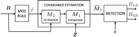
Figure 1: Three-stage Detection Architectures.

The first strategy relies on a three-stage detection architecture (depicted in Figure 1) where the first two stages (actually, the second stage consists of two sub-blocks) are devoted to the estimation of $\mbox{\boldmath{$M$}}_{1}$ (and $\mbox{\boldmath{$M$}}_{2}$) and incorporate the Information-based MOS rules [38]. More precisely, the first stage provides an estimate of $r$ and feeds the second stage which is responsible for the estimation of $\mbox{\boldmath{$M$}}_{2}$ and $\mbox{\boldmath{$M$}}_{1}$ according to Algorithm 1. The third stage accomplishes the detection task.

The second approach consists in a modification of the maximum likelihood estimation of $\mbox{\boldmath{$M$}}_{2}$ which accounts for the significant hop in the order of magnitude of the eigenvalues of $\mbox{\boldmath{$R$}}\mbox{\boldmath{$R$}}^{\dagger}$ when NLJs are present (a point better explained in Subsection III-A2). This discontinuity can be justified by noticing that common JNR values are in the range $[30,60]$ dB [41]. It follows that $r$ can be estimated by detecting this hop in magnitude.

III-A1 Three-stage Detection Architectures relying on Information-based MOS Rules

A block scheme of the proposed architectures is depicted in Figure 1: the first two blocks perform the estimates of $\mbox{\boldmath{$M$}}_{2}$ and $\mbox{\boldmath{$M$}}_{1}$ exploiting Information-based MOS rules for selecting $r$. The last block represents the final detection step. Here, it is important to note that to estimate $r$ the MLA fails because the hypotheses are nested and the likelihood function monotonically increases with $r$. Thus, focusing on the first block, the estimation of $r$ is accomplished exploiting the MOS rules which balance the growth of the likelihood function by means of a penalty term. Specifically, we consider the Akaike Information Criterion (AIC), the Bayesian Information Criterion (BIC), and the Generalized Information Criterion (GIC) [38]. Following the lead of [42, Ch.7], it is possible to show that, when $r$ is known, the number of unknown parameters of the distribution of $R$ is $k_{p}(r)=r(2N-r)+1$. As a consequence, the mentioned MOS rules can be expressed as

$$\hat{r}=\underset{r\in\{0,...,{N_{nj}^{max}}\}}{\arg\min}\{-2l(\mbox{\boldmath{$R$}},r)+p(r)\},$$ (11)

where $N_{nj}^{max}$ is the maximum number of jammers and

$$l(\mbox{\boldmath{$R$}},r)=-MN\log\pi-M\sum_{i=1}^{r}\log\frac{\gamma_{1,i}}{M}-M(N-r)\log\left[\frac{1}{M(N-r)}\sum_{i=r+1}^{N}\gamma_{1,i}\right]-MN$$ (12)

is the compressed log-likelihood of $R$ assuming that $r$ is known and $p(r)=k_{p}(r)\nu$ is the penalty term. Finally, factor $\nu$ takes on the following values

$$\nu=\begin{cases}2,\quad&\textrm{AIC},\\ 1+\rho,\ \rho\geq 1,\quad&\textrm{GIC},\\ \ln M,\quad&\textrm{BIC}.\end{cases}$$ (14)

Once the estimate $\hat{r}$ is available, it can be used in place of $r$ in Appendix A to estimate $\mbox{\boldmath{$M$}}_{2}$. The resulting estimate of $\mbox{\boldmath{$M$}}_{2}$ is, subsequently, used to obtain $\widehat{\mbox{\boldmath{$M$}}}_{1}$ as shown in Appendix B.

The last block of the proposed architecture implements an adaptive decision rule, devised resorting to the two-step GLRT design criteria [6]. Specifically, we first compute the GLRT test assuming that $\mbox{\boldmath{$M$}}_{1}$ is known. Then, the fully adaptive detector is obtained by replacing $\mbox{\boldmath{$M$}}_{1}$ with a suitable estimate. According to the first step, the GLRT based on the CUT for known $\mbox{\boldmath{$M$}}_{1}$ is the following decision rule

$$\max\limits_{\alpha_{T}}\frac{f_{10}(\mbox{\boldmath{$z$}};\alpha_{T},0,0,\sigma^{2},\mbox{\boldmath{$M$}}_{nj},\mbox{\boldmath{$M$}}_{c})}{f_{00}(\mbox{\boldmath{$z$}};0,0,0,\sigma^{2},\mbox{\boldmath{$M$}}_{nj},\mbox{\boldmath{$M$}}_{c})}\mbox{$\begin{array}[]{c}\stackrel{{\scriptstyle\stackrel{{\scriptstyle\textstyle H_{1}}}{{\textstyle>}}}}{{\stackrel{{\scriptstyle\textstyle<}}{{\textstyle H_{0}}}}}\end{array}$}\eta,$$ (15)

where $f_{l0}(\mbox{\boldmath{$z$}};\ldots)$, $l=0,1$, is defined by (4) and $\eta$ is the detection threshold value to be set according to the desired $P_{fa}$. It is not difficult to prove that (15) is statistically equivalent to

$$\frac{|\mbox{\boldmath{$z$}}^{{\dagger}}\mbox{\boldmath{$M$}}_{1}^{-1}\mbox{\boldmath{$v$}}(\theta_{T})|^{2}}{\mbox{\boldmath{$v$}}^{{\dagger}}(\theta_{T})\mbox{\boldmath{$M$}}_{1}^{-1}\mbox{\boldmath{$v$}}(\theta_{T})}\mbox{$\begin{array}[]{c}\stackrel{{\scriptstyle\stackrel{{\scriptstyle\textstyle H_{1}}}{{\textstyle>}}}}{{\stackrel{{\scriptstyle\textstyle<}}{{\textstyle H_{0}}}}}\end{array}$}\eta.$$ (16)

Finally, the adaptivity is achieved replacing $\mbox{\boldmath{$M$}}_{1}$ in (16) with the estimate (10) to come up with

$$\frac{|\mbox{\boldmath{$z$}}^{{\dagger}}\widehat{\mbox{\boldmath{$M$}}}_{1}^{-1}\mbox{\boldmath{$v$}}(\theta_{T})|^{2}}{\mbox{\boldmath{$v$}}^{{\dagger}}(\theta_{T})\widehat{\mbox{\boldmath{$M$}}}_{1}^{-1}\mbox{\boldmath{$v$}}(\theta_{T})}\mbox{$\begin{array}[]{c}\stackrel{{\scriptstyle\stackrel{{\scriptstyle\textstyle H_{1}}}{{\textstyle>}}}}{{\stackrel{{\scriptstyle\textstyle<}}{{\textstyle H_{0}}}}}\end{array}$}\eta.$$ (17)

For future reference, we refer to the above decision rule as Improved Double-Trained Adaptive Matched Filter (IDT-AMF), whereas we call the three-stage architectures coupling the name of the MOS rule used to estimate $r$ and the acronym IDT-AMF. For instance, when BIC is part of the architecture, we refer to the latter as IDT-AMF-BIC.

III-A2 Two-Stage Architecture based upon an Ad Hoc MLE of $\mbox{\boldmath{$M$}}_{2}$

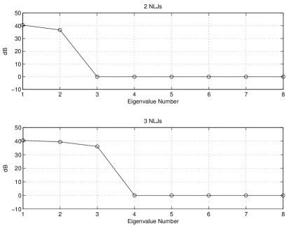
Figure 2: Eigenvalues of $\mbox{\boldmath{$M$}}_{2}$ in the presence of NLJs assuming $N=8$ and JNR$=30$ dB for all NLJs.

In the following, we propose a modification of the previously described three-stage architectures which consists in removing the block responsible for the estimate of $r$ and incorporating this feature in the block that returns the estimates of $\mbox{\boldmath{$M$}}_{1}$ and $\mbox{\boldmath{$M$}}_{2}$ through a heuristic MOS rule. To this end, let us remind that the goal of NLJs is to increase the power noise level within the victim radar making the adaptive threshold as high as possible with the result of masking the platforms under protection. This fact has some implications for the eigenvalues of the ICM which can be suitably exploited to estimate $r$. To have a clear vision of this situation, in Figure 2 we plot the eigenvalues of $\mbox{\boldmath{$M$}}_{2}$ (which is the true ICM) for $N_{nj}=2,3$ NLJs sharing JNR$=30$ dB. Inspection of the figure highlights that the presence of NLJs breaks down the eigenvalue set of $\mbox{\boldmath{$M$}}_{2}$ introducing a dramatic drop in magnitude.

The above behavior comes in handy to estimate the model order $r$ by thresholding the difference in magnitude between consecutive eigenvalues of $\mbox{\boldmath{$S$}}_{2}=\frac{1}{M}\mbox{\boldmath{$R$}}\mbox{\boldmath{$R$}}^{{\dagger}}$, starting from the lowest values. Specifically, let $\gamma_{1,1}/M\geq\gamma_{1,2}/M\geq...\geq\gamma_{1,N}/M$ be the eigenvalues of $\mbox{\boldmath{$S$}}_{2}$, then the estimation of $r$ is described in Algorithm 2, where $\eta$ is a threshold whose value reflects the difference in magnitude between the eigenvalues associated with both NLJs and thermal noise and those representative of the thermal noise only. Notice that the underlying decision problem solved by this approach is

$$\begin{cases}H_{1}^{{}^{\prime\prime}}:\mbox{\boldmath{$r$}}_{m}\sim\mbox{$\mathcal{C}$}\mbox{$\mathcal{N}$}_{N}({\mbox{\boldmath$0$}},\sigma^{2}\mbox{\boldmath{$I$}}+\mbox{\boldmath{$M$}}_{nj}),&m=1,\ldots,M,\\ H_{0}^{{}^{\prime\prime}}:\mbox{\boldmath{$r$}}_{m}\sim\mbox{$\mathcal{C}$}\mbox{$\mathcal{N}$}_{N}({\mbox{\boldmath$0$}},\sigma^{2}\mbox{\boldmath{$I$}}),&m=1,\ldots,M,\end{cases}$$ (18)

where the rank of $\mbox{\boldmath{$M$}}_{nj}$ is unknown. It turns out that, under $H_{0}^{{}^{\prime\prime}}$, the unknown parameter is $\sigma^{2}$, which must be estimated in order to set the detection threshold. To this end, several strategies are possible. For instance, a lookup table can be filled up off-line by measuring the thermal noise power under different operating conditions. Then, each entry of this table could be used when the system is in operation. An alternate approach might consist in scheduling a collection of noisy samples when the antenna is disengaged and exploiting such samples to estimate the noise power.

Finally, once $r$ has been estimated, $\widehat{\mbox{\boldmath{$M$}}}_{2}$ can be obtained as described in Appendix A and the IDT-AMF is applied. In the following, we call this architecture Eigenvalue-based IDT-AMF and we use the abbreviation IDT-AMF-EIG.

Algorithm 2 Estimation Procedure for $r$

0:  $\eta$, $\gamma_{1,1}/M\geq\gamma_{1,2}/M\geq...\gamma_{1,N}/M>0$

0:  $\widehat{r}$

1:  Set $i=N-1$, $\hat{r}=0$

2:  Compute $\Delta_{i}=\frac{1}{M}(\gamma_{1,i}-\gamma_{1,i+1})$

3:  If $\Delta_{i}>\eta$, then $\hat{r}=i$ and go to step 6 else go to step 4

4:  Set $i=i-1$

5:  If $i\geq 1$ go to step 2 else go to step 6

6:  Return $\widehat{r}$

III-B NLJs and Coherent Interferers Joint Attack

In this subsection, we focus on problem (2) and devise an architecture capable of detecting point-like targets assuming that noise-like jammers as well as coherent interferers contaminate the echoes from the CUT. Specifically, such architecture consists of a covariance estimation stage, which relies on the results obtained in Section III-A1, followed by a new detection stage which incorporates a sparse reconstruction algorithm. This choice is dictated by the fact that problem (2) hides an inherent sparse nature, which can be drawn by means of a suitable reformulation. Thus, we select the so-called SLIM algorithm as sparse reconstruction algorithm since it provides a good trade off between computational requirements and reconstruction performance [39].

Let us consider the hypothesis $H_{1,1}$, defined in (2), where it is assumed that a number of coherent interferers ($N_{q}$) are present together with the NLJs and note that $z$ is the sum of three components

$$\mbox{\boldmath{$z$}}=\alpha_{T}\mbox{\boldmath{$v$}}(\theta_{T})+\sum_{i=1}^{N_{q}}\beta_{i}\mbox{\boldmath{$v$}}(\theta_{q,i})+\mbox{\boldmath{$n$}}.$$ (19)

To effectively apply the SLIM approach, it is necessary to bring to light the sparse nature of (19) recasting the above equation as a standard sparse model. From an intuitive point of view, note that radar system steers the beam along several directions to cover the surveillance area, but backscattered echoes and/or interfering signals hit the system from a few directions only. With this remark in mind, let us sample the angular sector under surveillance and form a discrete and finite set of angles denoted by $\Theta=\left\{\theta_{1},\ldots,\theta_{L}\right\}$, $\theta_{1}\leq\theta_{2}\leq\ldots\leq\theta_{L}$. Moreover, we assume that the target nominal angle $\theta_{T}$ and the AOA of possible $N_{q}\ll L$ coherent interferers belong to $\Theta$. Thus, if we define $\mbox{\boldmath{$V$}}=[\mbox{\boldmath{$v$}}(\theta_{1}),...,\mbox{\boldmath{$v$}}(\theta_{L})]\in\mathbb{C}^{N\times L}$ as the model matrix whose columns are the steering vectors associated with the angular positions $\left\{\theta_{1},...,\theta_{L}\right\}$ and a vector $\mbox{\boldmath{$\alpha$}}=[\alpha_{1},...,\alpha_{L}]^{T}\in\mathbb{C}^{L\times 1}$ whose nonzero entries correspond to the AOAs of the target and the coherent interferers in $V$, then it is possible to recast $z$ as

$$\mbox{\boldmath{$z$}}=\mbox{\boldmath{$V$}}\mbox{\boldmath{$\alpha$}}+\mbox{\boldmath{$n$}},$$ (20)

where $\alpha$ is assumed to contain the target response $\alpha_{T}$ as well as the magnitudes of the coherent jammers $\left\{\beta\right\}_{i=1}^{N_{q}}$. It is important to observe that since $N_{q}\ll L$, then $\alpha$ is a sparse vector. In fact, from (20), it turns out that only $N_{q}+1$ components of $\alpha$ are possibly different from zero. In this case, the SLIM algorithm can be used to produce a very accurate representation for the scene of interest. Remarkably, we can exploit the sparse estimate returned by the SLIM to address the following classification problem

• target plus noise-like interferers hypothesis:

  $$\mbox{$\mathcal{H}$}_{1}:\ \mbox{\boldmath{$z$}}=\alpha_{T}\mbox{\boldmath{$v$}}(\theta_{T})+\mbox{\boldmath{$n$}};$$ (21)

• noise-like plus coherent interferers hypothesis:

  $$\mbox{$\mathcal{H}$}_{2}:\ \mbox{\boldmath{$z$}}=\sum_{i=1}^{N_{q}}\beta_{i}\mbox{\boldmath{$v$}}(\theta_{q,i})+\mbox{\boldmath{$n$}};$$ (22)

• target plus noise-like and coherent interferers hypothesis:

  $$\mbox{$\mathcal{H}$}_{3}:\ \mbox{\boldmath{$z$}}=\alpha_{T}\mbox{\boldmath{$v$}}(\theta_{T})+\sum_{i=1}^{N_{q}}\beta_{i}\mbox{\boldmath{$v$}}(\theta_{q,i})+\mbox{\boldmath{$n$}}.$$ (23)

Thus, as shown in what follows, the newly proposed architecture exhibits, as a byproduct, signal classification capabilities. Let us start the design by writing the LRT based upon the CUT

$$\Lambda(\mbox{\boldmath{$z$}};\mbox{\boldmath{$\alpha$}},\mbox{\boldmath{$M$}}_{1})=\frac{f_{1}(\mbox{\boldmath{$z$}};\mbox{\boldmath{$\alpha$}},\mbox{\boldmath{$M$}}_{1},H_{1,1})}{f_{0}(\mbox{\boldmath{$z$}};{\mbox{\boldmath$0$}},\mbox{\boldmath{$M$}}_{1},H_{0,0})}\mbox{$\begin{array}[]{c}\stackrel{{\scriptstyle\stackrel{{\scriptstyle\textstyle H_{1,1}}}{{\textstyle>}}}}{{\stackrel{{\scriptstyle\textstyle<}}{{\textstyle H_{0,0}}}}}\end{array}$}\eta,$$ (24)

where $f_{l}(\mbox{\boldmath{$z$}};l\mbox{\boldmath{$\alpha$}},\mbox{\boldmath{$M$}}_{1},H_{l,l})$ is the pdf of $z$ under $H_{l,l}$, $l=0,1$, whose expression is

$$f_{l}(\mbox{\boldmath{$z$}};l\mbox{\boldmath{$\alpha$}},\mbox{\boldmath{$M$}}_{1},H_{l,l})=\frac{1}{\pi^{N}\det(\mbox{\boldmath{$M$}}_{1})}\exp\{-\mbox{\rm tr}\,[\mbox{\boldmath{$M$}}_{1}^{-1}(\mbox{\boldmath{$z$}}-l\mbox{\boldmath{$V$}}\mbox{\boldmath{$\alpha$}})(\mbox{\boldmath{$z$}}-l\mbox{\boldmath{$V$}}\mbox{\boldmath{$\alpha$}})^{\dagger}]\}.$$ (25)

Now, note that decision rule (24) is not of practical interest since both $\alpha$ and $\mbox{\boldmath{$M$}}_{1}$ are not known and, hence, must be estimated from data. As already stated at the beginning of this subsection, the estimate of $\mbox{\boldmath{$M$}}_{1}$ can be accomplished using the procedures described in Algorithm 1. As for $\alpha$, it is estimated resorting to the framework proposed in [39]. Specifically, let us assume that $\alpha$ is a random vector independent of the noise component and that obeys a prior promoting the sparsity, given by

$$f(\mbox{\boldmath{$\alpha$}};q)=\frac{1}{C}\prod\limits_{i=1}^{L}\exp{\left\{-\frac{2}{q}\left(|\alpha_{i}|^{q}-1\right)\right\}},$$ (26)

where $C$ is a normalization constant and $q\in\Omega_{q}=(0,1]$ is a tuning parameter (smaller values of $q$ correspond to sharper peak of the prior distribution and consequently sparser estimate of $\alpha$). Then, $\alpha$ is estimated solving the following maximization problem

$$\max\limits_{\mbox{\boldmath{$\alpha$}}}f_{1}(\mbox{\boldmath{$z$}};\widehat{\mbox{\boldmath{$M$}}}_{1},H_{1,1}|\mbox{\boldmath{$\alpha$}})f(\mbox{\boldmath{$\alpha$}};q),$$ (27)

where $f_{1}(\mbox{\boldmath{$z$}};\widehat{\mbox{\boldmath{$M$}}}_{1},H_{1,1}|\mbox{\boldmath{$\alpha$}})$ is the conditional pdf of $z$ given $\alpha$. Taking the negative logarithm, problem (27) is equivalent to

$$\min_{\mbox{\boldmath{$\alpha$}}}\underbrace{\left\{\|\mbox{\boldmath{$y$}}-\mbox{\boldmath{$A$}}\mbox{\boldmath{$\alpha$}}\|_{2}^{2}+\sum\limits_{i=1}^{L}\frac{2}{q}\left(|\alpha_{i}|^{q}-1\right)\right\}}_{g_{q}(\mbox{\boldmath{$\alpha$}})}$$ (28)

where $\mbox{\boldmath{$A$}}=\widehat{\mbox{\boldmath{$M$}}}_{1}^{-1/2}\mbox{\boldmath{$V$}}$ and $\mbox{\boldmath{$y$}}=\widehat{\mbox{\boldmath{$M$}}}_{1}^{-1/2}\mbox{\boldmath{$z$}}$. Notice that the first addendum of $g_{q}(\mbox{\boldmath{$\alpha$}})$ corresponds to a fitting term, whereas the second term promotes sparsity. Setting to zero the first derivative of $g_{q}(\mbox{\boldmath{$\alpha$}})$ with respect to $\alpha$ leads to

$$\frac{d}{d\mbox{\boldmath{$\alpha$}}}[g_{q}(\mbox{\boldmath{$\alpha$}})]=\mbox{\boldmath{$A$}}^{\dagger}\mbox{\boldmath{$A$}}\mbox{\boldmath{$\alpha$}}-\mbox{\boldmath{$A$}}^{\dagger}\mbox{\boldmath{$y$}}+\mbox{\boldmath{$P$}}_{q}^{-1}\mbox{\boldmath{$\alpha$}}={\mbox{\boldmath$0$}},$$ (30)

where $\mbox{\boldmath{$P$}}_{q}=\mbox{\boldmath\bf diag}\,{(\mbox{\boldmath{$p$}}_{q})}$, with $\mbox{\boldmath{$p$}}_{q}=[|\alpha_{1}|^{2-q},|\alpha_{2}|^{2-q},...,|\alpha_{L}|^{2-q}]^{T}$. Supposing that an initial estimate of $\alpha$ is available, it is possible to apply a cyclic optimization procedure as in [39], and the step at the $(m)$th iteration can be expressed as

$$\mbox{\boldmath{$\alpha$}}_{q}^{(m)}=\mbox{\boldmath{$P$}}_{q}^{(m-1)}\mbox{\boldmath{$A$}}^{\dagger}\left(\mbox{\boldmath{$A$}}\mbox{\boldmath{$P$}}_{q}^{(m-1)}\mbox{\boldmath{$A$}}^{\dagger}+\mbox{\boldmath{$I$}}\right)^{-1}\mbox{\boldmath{$y$}},$$ (31)

given $\mbox{\boldmath{$P$}}_{q}^{(m-1)}=\mbox{\boldmath\bf diag}\,(\mbox{\boldmath{$p$}}_{q}^{(m-1)})$ from the $(m-1)$th iteration. The optimization procedure can terminate after a fixed number of iterations or when the following convergence criterion is satisfied

$$\frac{\|\mbox{\boldmath{$\alpha$}}_{q}^{(m)}-\mbox{\boldmath{$\alpha$}}_{q}^{(m-1)}\|_{2}}{\|\mbox{\boldmath{$\alpha$}}_{q}^{(m)}\|_{2}}<\Delta,$$ (32)

with $\Delta$ a suitable small positive number. As for the initial value of $\alpha$, a possible choice is

$$\alpha_{i}^{(0)}=\frac{\mbox{\boldmath{$v$}}(\theta_{i})^{\dagger}\widehat{\mbox{\boldmath{$M$}}}_{1}^{-1}\mbox{\boldmath{$z$}}}{\mbox{\boldmath{$v$}}(\theta_{i})^{\dagger}\widehat{\mbox{\boldmath{$M$}}}_{1}^{-1}\mbox{\boldmath{$v$}}(\theta_{i})},\quad i=1,\ldots,L.$$ (33)

It still remains to estimate $q\in\Omega_{q}$. As a preliminary step, we sample $\Omega_{q}$ to come up with a finite set of admissible values for $q$ denoted by $\bar{\Omega}_{q}$. Now, given $q\in\bar{\Omega}_{q}$, let $\tilde{\mbox{\boldmath{$\alpha$}}}_{q}$ be the estimate of $\alpha$ provided by the above iterative procedure, summarized in Algorithm 3, and estimate the number of peaks, $h(q)$ say, in $\tilde{\mbox{\boldmath{$\alpha$}}}_{q}$ as follows

1. sort the entries of $\tilde{\mbox{\boldmath{$\alpha$}}}_{q}$ from the largest to the smallest;

2. select $h(q)$ returning the lowest value of $\mbox{BIC}_{q}=2\|\mbox{\boldmath{$y$}}-{\mbox{\boldmath{$A$}}}\widehat{\mbox{\boldmath{$\alpha$}}}_{q}\|_{2}^{2}+3h(q)\log\left(2N\right)$, where $3h(q)$ is the number of parameters to be estimated (namely, azimuth and complex amplitude for each active peaks) and $\widehat{\mbox{\boldmath{$\alpha$}}}_{q}$ is the least-squares estimate for the selected peaks setting to zero the other entries of $\alpha$ (denote by $\bar{\mbox{\boldmath{$\alpha$}}}_{q}$ the final estimate of $\mbox{\boldmath{$\alpha$}}_{q}$).

As a result, we obtain the set $\{\mbox{BIC}_{q}:q\in\bar{\Omega}_{q}\}$ and the estimate of $q$ is obtained as $\widehat{q}=\arg\min_{q\in\bar{\Omega}_{q}}\mbox{BIC}_{q}$.

Algorithm 3 Sparse Learning Iterative Minimization (SLIM)

0:  $\Delta>0$, $q\in(0,1]$, $A$, $y$

0:  $\tilde{\mbox{\boldmath{$\alpha$}}}_{q}$

1:  Set $m=0$, $\mbox{\boldmath{$\alpha$}}^{(0)}=\left[\frac{\mbox{\boldmath{$v$}}(\theta_{1})^{\dagger}\widehat{\mbox{\boldmath{$M$}}}_{1}^{-1}\mbox{\boldmath{$z$}}}{\mbox{\boldmath{$v$}}(\theta_{1})^{\dagger}\widehat{\mbox{\boldmath{$M$}}}_{1}^{-1}\mbox{\boldmath{$v$}}(\theta_{1})},\ldots,\frac{\mbox{\boldmath{$v$}}(\theta_{L})^{\dagger}\widehat{\mbox{\boldmath{$M$}}}_{1}^{-1}\mbox{\boldmath{$z$}}}{\mbox{\boldmath{$v$}}(\theta_{L})^{\dagger}\widehat{\mbox{\boldmath{$M$}}}_{1}^{-1}\mbox{\boldmath{$v$}}(\theta_{L})}\right]^{T}$,

2:  Set $m=m+1$

3:  Compute $\mbox{\boldmath{$P$}}_{q}^{(m-1)}=\mbox{\boldmath\bf diag}\,(\mbox{\boldmath{$p$}}_{q}^{(m-1)})$, with $\mbox{\boldmath{$p$}}_{q}^{(m-1)}=\left[|\alpha_{1}^{(m-1)}|^{2-q},|\alpha_{2}^{(m-1)}|^{2-q},...,|\alpha_{L}^{(m-1)}|^{2-q}\right]^{T}$

4:  Compute $\mbox{\boldmath{$\alpha$}}^{(m)}=\mbox{\boldmath{$P$}}_{q}^{(m-1)}\mbox{\boldmath{$A$}}^{\dagger}\left(\mbox{\boldmath{$A$}}\mbox{\boldmath{$P$}}_{q}^{(m-1)}\mbox{\boldmath{$A$}}^{\dagger}+\mbox{\boldmath{$I$}}\right)^{-1}\mbox{\boldmath{$y$}}$

5:  If ${\|\mbox{\boldmath{$\alpha$}}^{(m)}-\mbox{\boldmath{$\alpha$}}^{(m-1)}\|_{2}}/{\|\mbox{\boldmath{$\alpha$}}^{(m)}\|_{2}}<\Delta$ go to step 6 else go to step 2

6:  Return $\tilde{\mbox{\boldmath{$\alpha$}}}_{q}=\mbox{\boldmath{$\alpha$}}^{(m)}$.

Finally, the adaptive LRT can be written as

$$\frac{f_{11}(\mbox{\boldmath{$z$}};\bar{\mbox{\boldmath{$\alpha$}}}_{\hat{q}},\widehat{\mbox{\boldmath{$M$}}}_{1},H_{1,1})}{f_{00}(\mbox{\boldmath{$z$}};{\mbox{\boldmath$0$}},\widehat{\mbox{\boldmath{$M$}}}_{1},H_{0,0})}\mbox{$\begin{array}[]{c}\stackrel{{\scriptstyle\stackrel{{\scriptstyle\textstyle H_{1,1}}}{{\textstyle>}}}}{{\stackrel{{\scriptstyle\textstyle<}}{{\textstyle H_{0,0}}}}}\end{array}$}\eta.$$ (34)

Before concluding this section, we discuss the classification capabilities raising from $\bar{\mbox{\boldmath{$\alpha$}}}_{\hat{q}}$. Specifically, let us recall that $H_{1,1}$ can be viewed as the union of three hypotheses, namely $H_{1,1}=\cup_{i=1}^{3}\mbox{$\mathcal{H}$}_{i}$. Now, in order to mitigate the presence of false objects (ghosts) introduced by $\bar{\mbox{\boldmath{$\alpha$}}}_{\hat{q}}$ and to merge contiguous estimates (induced by energy spillover), we partition the set $\Theta$ into $N_{s}$ subsets, $\Theta_{i}$ say, containing contiguous AOAs. In addition, for simplicity, we assume that $|\Theta|/N_{s}=|\Theta_{1}|=\ldots=|\Theta_{N_{s}}|=N_{\theta}\in{\mathds{N}}$, namely that all the subsets share the same number of contiguous AOAs. As a consequence, the generic subset can be written as

$$\Theta_{i}=\{\theta_{(i-1)N_{\theta}+1},\ldots,\theta_{iN_{\theta}}\},\ i=1,\ldots,N_{s}.$$ (35)

Since the target AOA, $\theta_{T}$ say, is supposed to belong to $\Theta$, then there exists $\bar{i}\in\{1,\ldots,N_{s}\}$ such that $\theta_{T}\in\Theta_{\bar{i}}$ and let us denote this subset as $\Theta_{T}$ ($=\Theta_{\bar{i}}$). Thus, for classification purposes, we say that a generic subset $\Theta_{i}$, $i\in\{1,\ldots,N_{s}\}$, contains coherent components if there exists at least an index $l\in\{1,\ldots,L\}$ such that

$$\bar{\mbox{\boldmath{$\alpha$}}}_{\hat{q}}(l)\neq 0\quad\mbox{and}\quad\theta_{l}\in\Theta_{i}.$$ (36)

The above partitioning procedure allows us to define new vectors, $\gamma$ and $\bar{\mbox{\boldmath{$\gamma$}}}_{\hat{q}}$ say, of size $N_{s}$ starting from $\alpha$ and $\bar{\mbox{\boldmath{$\alpha$}}}_{\hat{q}}$, respectively, that contain information about the angular location in terms of $\Theta_{i}$ of the coherent signals received by the system. Such vectors will be used at the analysis stage to quantify the algorithm capability in drawing a picture of the entire operating scenario. Specifically, $\forall i\in\{1,\ldots,N_{s}\}$, we set

• $\mbox{\boldmath{$\gamma$}}(i)=1$ if condition (36) applied to $\alpha$ holds, otherwise $\mbox{\boldmath{$\gamma$}}(i)=0$;

• $\bar{\mbox{\boldmath{$\gamma$}}}_{\hat{q}}(i)=1$ if (36) is valid, otherwise $\bar{\mbox{\boldmath{$\gamma$}}}_{\hat{q}}(i)=0$.

Then, denoting by $\Omega_{\gamma}$, with $|\Omega_{\gamma}|\geq 1$, the set of integers indexing the nonzero entries of $\bar{\mbox{\boldmath{$\gamma$}}}_{\hat{q}}$, we can reason according to the following rationale

• if data contain only one coherent component ($|\Omega_{\gamma}|=1$), which can be due to either an interferer or a target, then there exists $\tilde{i}\in\{1,\dots,N_{s}\}$ such that $\Omega_{\gamma}=\{\tilde{i}\}$ (namely, $\bar{\mbox{\boldmath{$\gamma$}}}_{\hat{q}}(\tilde{i})\neq 0$ and $\bar{\mbox{\boldmath{$\gamma$}}}_{\hat{q}}(i)=0$, $\forall i\neq\tilde{i}$) and two cases can occur

  • Case 1: $\Theta_{\tilde{i}}=\Theta_{T}$, which implies that $\mbox{$\mathcal{H}$}_{1}$ holds true;

  • Case 2: $\Theta_{\tilde{i}}\neq\Theta_{T}$, which implies that $\mbox{$\mathcal{H}$}_{2}$ is in force;

• if data contain more than one coherent component ($|\Omega_{\gamma}|>1$), which can be generated by jammers or the target, then the following cases have to be accounted for

  • Case 1: $\exists\tilde{i}\in\Omega_{\gamma}$ such that $\Theta_{\tilde{i}}=\Theta_{T}$; in this case $\mbox{$\mathcal{H}$}_{3}$ is declared;

  • Case 2: $\forall\tilde{i}\in\Omega_{\gamma}$: $\Theta_{\tilde{i}}\neq\Theta_{T}$; in this case $\mbox{$\mathcal{H}$}_{2}$ is declared.

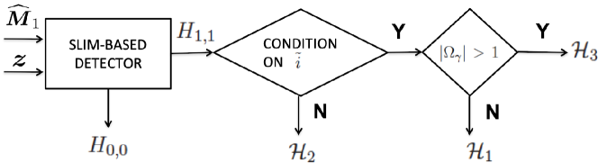
Figure 3: Block scheme of the SLIM-based detection architecture.

Finally, the SLIM-based detector (34) can be incorporated into the architecture depicted in Figure 3, where the condition on $\tilde{i}$ clearly is: $\exists\ \tilde{i}\in\Omega_{\gamma}:\Theta_{\tilde{i}}=\Theta_{T}$. It is important to highlight that such architecture can absolve the functions of both SLB and SLC [2]. In fact, the use of $\widehat{\mbox{\boldmath{$M$}}}_{1}$ allows to place nulls along the NLJ directions, while $\bar{\mbox{\boldmath{$\alpha$}}}_{\hat{q}}$ allows to separate the target response from the coherent interferers.

Summarizing, the proposed approach allows to suitably handle situations where NLJs as well as CJs attack the victim radar providing a tool for the discrimination between useful structured returns and unwanted signals. In fact, focusing on the CUT only, the actual classification problem herein addressed is the following multiple-hypothesis test

$$\left\{\begin{array}[]{l}\mbox{$\mathcal{H}$}_{1}:\mbox{\boldmath{$z$}}=\alpha_{T}\mbox{\boldmath{$v$}}(\theta_{T})+\mbox{\boldmath{$n$}},\\ \mbox{$\mathcal{H}$}_{2}:\mbox{\boldmath{$z$}}=\sum\limits_{i=1}^{N_{q}}\beta_{i}\mbox{\boldmath{$v$}}(\theta_{q,i})+\mbox{\boldmath{$n$}},\\ \mbox{$\mathcal{H}$}_{3}:\mbox{\boldmath{$z$}}=\alpha_{T}\mbox{\boldmath{$v$}}(\theta_{T})+\sum\limits_{i=1}^{N_{q}}\beta_{i}\mbox{\boldmath{$v$}}(\theta_{q,i})+\mbox{\boldmath{$n$}},\\ H_{00}:\mbox{\boldmath{$z$}}=\mbox{\boldmath{$n$}}.\end{array}\right.$$ (37)

IV Illustrative Examples

In this section, we analyze the performance of the new ECCM strategies against the disturbance injected by NLJs and/or CJs through the antenna sidelobes. Specifically, in Subsection IV-A, we analyze the performance in the first scenario (NLJ-only attack) while in Subsection IV-B, we investigate the behavior of the SLIM-based detector when both NLJs and CJs are present.

IV-A NLJ-only Case

In this section, we present illustrative examples assessing the performance of the multi-stage architectures devised in Section III-A in terms of $P_{d}$ against the SINR. For comparison purpose, we also report the $P_{d}$ curves of the so-called Double Trained-AMF (DT-AMF) introduced in [37], the IDT-AMF with known $r$, and the clairvoyant (non-adaptive) detector, i.e., the Matched Filter (MF) with known $\mbox{\boldmath{$M$}}_{1}$, which represents an upper bound to the detection performance. The numerical examples are obtained resorting to standard Monte Carlo counting techniques. More precisely, the $P_{d}$ is estimated over $10^{3}$ independent trials, whereas the detection thresholds are computed exploiting $100/P_{fa}$ independent trials. In all the illustrative examples, we set $N=16$, $\sigma^{2}=1$, $d=\lambda/2$, and $P_{fa}=10^{-4}$. The SINR is defined as $\textrm{SINR}=|\alpha|^{2}\mbox{\boldmath{$v$}}(0)^{\mathrm{{\dagger}}}\mbox{\boldmath{$M$}}_{1}^{-1}\mbox{\boldmath{$v$}}(0)$, while the considered scenario comprises three NLJs with the same power from the following AOAs: $\theta_{nj,1}=15^{\circ}$, $\theta_{nj,2}=25^{\circ}$, and $\theta_{nj,3}=-10^{\circ}$. Then, the resulting ICMs are given by $\mbox{\boldmath{$M$}}_{2}=\mbox{\boldmath{$I$}}+\sum_{i=1}^{3}\textrm{JNR}\ \mbox{\boldmath{$v$}}(\theta_{nj,i})\mbox{\boldmath{$v$}}(\theta_{nj,i})^{{\dagger}}$ and $\mbox{\boldmath{$M$}}_{1}=\mbox{\boldmath{$M$}}_{2}+\textrm{CNR}\ \mbox{\boldmath{$M$}}_{c}$. The $(i,j)$th entry of $\mbox{\boldmath{$M$}}_{c}$ is given by $\mbox{\boldmath{$M$}}_{c}(i,j)=\rho^{|i-j|}$, where $\rho=0.9$ is the one-lag correlation coefficient. Finally, the maximum number of NLJs is set to $N/2$ and the GIC parameter, $\rho$ say, is equal to 2 (this choice represents a reasonable compromise to limit the model overestimation).

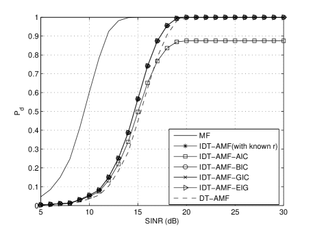
Figure 4: $P_{d}$ versus SINR for the MF, IDT-AMF, IDT-AMF-AIC, IDT-AMF-BIC, IDT-AMF-GIC, IDT-AMF-EIG and DT-AMF assuming $N=16$, $K=M=20$, CNR=20 dB and JNR=30 dB.

In Figure 4, the $P_{d}$ versus SINR for all the considered detectors is plotted assuming $K=M=20$, JNR $=30$ dB and CNR $=20$ dB. As it can be seen, the IDT-AMF-BIC, IDT-AMF-GIC and IDT-AMF-EIG have nearly the same performance as the IDT-AMF with known $r$ and they exhibit higher $P_{d}$ values than the DT-AMF with a gain of 0.6 dB at $P_{d}=0.9$. The IDT-AMF-BIC, IDT-AMF-GIC, IDT-AMF-EIG and IDT-AMF exhibit similar performances due to the fact that the stages responsible for the estimate of $r$ share the same estimation accuracy. As to the IDT-AMF-AIC, it experiences a loss about 1.0 dB at $P_{d}=0.8$ with respect to other proposed detectors but still has slightly higher $P_{d}$ than the DT-AMF in the low/medium SINR region. However, the IDT-AMF-AIC is not capable of achieving $P_{d}=1.0$ for higher SINR values at least for the considered parameter values.

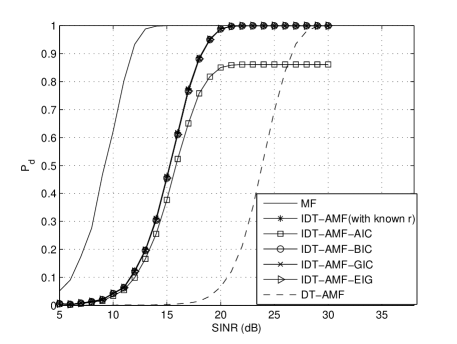
Figure 5: $P_{d}$ versus SINR for the MF, IDT-AMF, IDT-AMF-AIC, IDT-AMF-BIC, IDT-AMF-GIC, IDT-AMF-EIG and DT-AMF assuming $N=16$, $K=14$, $M=20$, CNR=20 dB and JNR=30 dB.

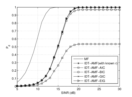
Figure 6: $P_{d}$ versus SINR for the MF, IDT-AMF, IDT-AMF-AIC, IDT-AMF-BIC, IDT-AMF-GIC, and IDT-AMF-EIG assuming $N=16$, $K=20$, $M=13$, CNR=20 dB and JNR=30 dB.

To show the influence of $K$ and $M$ on the detection performance of the proposed detectors, in Figure 5 we set $K=14$ leaving the other parameters as in Figure 4, whereas the parameter values in Figure 6 are the same as in Figure 4 but for $M=13$. Inspection of Figure 5 confirms the trend observed in Figure 4. Moreover, the performance gain of the proposed detectors with respect to the DT-AMF increases as $K$ decreases. Precisely, the DT-AMF experiences a loss of about 8.5 dB at $P_{d}=0.9$ with respect to the architectures based upon BIC, GIC, and the modified ML estimation. Even though the IDT-AMF-AIC performs better than the DT-AMF for SINR$<26$ dB, it is still not capable of ensuring $P_{d}=1$. Comparing Figure 5 with Figure 4, we can note that each proposed detector experiences a loss of about 1 dB when $K$ decreases from $20$ to $14$. This is due to the fact that the estimation quality of $r$ and $\mbox{\boldmath{$M$}}_{1}$ reduces. On the other hand, Figure 6 highlights that, when $M=13$ and $K=20$, the IDT-AMF-GIC and IDT-AMF-EIG overcome the IDT-AMF-BIC with a gain of 0.4 dB at $P_{d}=0.9$, whereas the IDT-AMF-AIC has a severe performance degradation. It is important to stress that the $P_{d}$ curve of DT-AMF is not reported in Figure 6 since it is not defined when $M<N$.

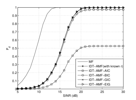
Figure 7: $P_{d}$ versus SINR for the MF, IDT-AMF, IDT-AMF-AIC, IDT-AMF-BIC, IDT-AMF-GIC and IDT-AMF-EIG assuming $N=16$, $K=14$, $M=13$, CNR=20 dB and JNR=30 dB.

Finally, in Figure 7, the $P_{d}$ performances are investigated assuming $K<N$ and $M<N$. In particular, we set $K=14$, $M=13$ and leave unaltered the other parameters. The curves in Figure 7 indicate that the detection performances of the IDT-AMF-GIC, IDT-AMF-EIG, and IDT-AMF are still similar while the IDT-AMF-BIC experience a performance degradation of about 0.5 dB at $P_{d}=0.9$.

Summarizing, architectures IDT-AMF-GIC, IDT-AMF-EIG, and IDT-AMF-BIC are effective solutions to detect point-like targets in the presence of an unknown number of NLJs, with IDT-AMF-GIC and IDT-AMF-EIG slightly superior to IDT-AMF-BIC. However, IDT-AMF-GIC requires to set a parameter while IDT-AMF-EIG exploits two thresholding stages. For this reason, the IDT-AMF-BIC emerges as a viable means for practical implementation.

IV-B SLIM-based detector performance analysis (NLJs and CJs joint attack)

In this subsection, we investigate the behavior of the SLIM-based detector in a scenario which assumes the joint presence of one NLJ and two CJs ($N_{q}=2$). It is important to note that CJs can be also categorized as targets, since they emulate echoes from an object of interest. For this reason, the considered performance metrics concern the capability of the system to detect both target and CJs and to discriminate between the echoes backscattered from the target and the echo-like signal transmitted by the CJs. The NLJ illuminates the radar with a JNR of $30$ dB and AOA $\theta_{nj}=10^{\circ}$, whereas the CJs are located at $\theta_{q,1}=-14^{\circ}$ and $\theta_{q,2}=16^{\circ}$ and radiate power at the same JNR of 45 dB. Target signature is given by $\mbox{\boldmath{$v$}}(0)$ and the SINR is defined as in the previous subsection. In other words, the operating scenario corresponds to $\mbox{$\mathcal{H}$}_{3}$. As for the ICMs, $\mbox{\boldmath{$M$}}_{2}=\mbox{\boldmath{$I$}}+\mbox{JNR}\mbox{\boldmath{$v$}}(\theta_{nj})\mbox{\boldmath{$v$}}(\theta_{nj})^{\dagger}$, whereas $\mbox{\boldmath{$M$}}_{1}$ is defined using the same parameters as in the previous subsection.

The analysis, conducted by means of Monte Carlo simulation, is aimed at estimating the following main performance metrics:

• the probability of detection ($P_{d}$) defined as the probability to declare $H_{1,1}$ when the latter holds true for a preassigned value of the $P_{fa}$, defined as the probability to declare $H_{1,1}$ when $H_{0,0}$ is in force;

• the probability of declaring the presence of a target under $\mbox{$\mathcal{H}$}_{3}$, which is denoted by $P_{t|H_{3}}$;

• the probabilities of correct classification, namely the probability of declaring $\mbox{$\mathcal{H}$}_{i}$, $i=1,2,3$, when it is on force.

Finally, to assess the estimation capabilities of the SLIM-based detector, additional figure of merits will be suitably introduced in the second part of this section. All the mentioned metrics are estimated resorting to $10^{3}$ independent trials, while the detection threshold is computed over $100/P_{fa}$ independent trials. An additional thresholding of the entries of $\bar{\mbox{\boldmath{$\alpha$}}}_{\hat{q}}$ is applied to mitigate as much as possible the number of false targets generated by the SLIM estimate especially at low SINR values. To this end, the threshold is set to ensure a probability of declaring the presence of a false target equal to 10^-2. Finally, all the numerical examples assume $N=16$, $P_{fa}=10^{-4}$, an angular sector under surveillance ranging from $-22^{\circ}$ to $22^{\circ}$ and uniformly sampled at $1$ degree (namely, $L=45$), and $|\Theta_{i}|=5$ with $\Theta_{T}=\{-2,\ldots,2\}$.

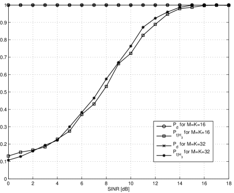
Figure 8: Performance of the SLIM-based detector in terms of $P_{d}$ and $P_{t|H_{3}}$ versus SINR for $M=K=16$ and $M=K=32$.

In Figure 8, we show the $P_{d}$ and the $P_{t|H_{3}}$ both as functions of the SINR and for $(K,M)\in\{(16,16),(32,32)\}$. As expected, the $P_{d}$ is equal to $1$ regardless the values of $K$, $M$, and SINR. This is due to the presence of the CJs whose JNR is constant and equal to $45$ dB. On the other hand, the $P_{t|H_{3}}$ achieves $1$ at SINR$=15$ dB when $(K,M)=(32,32)$ and at SINR$=17$ dB when $(K,M)=(16,16)$. Generally speaking, inspection of the figure highlights that increasing the volume of training samples leads to a moderate improvement of the $P_{t|H_{3}}$.

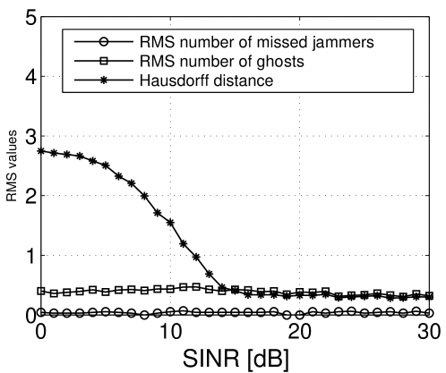
Figure 9: RMS values of $n_{mj}$, $n_{g}$, and $h_{d}(\cdot,\cdot)$ assuming $M=K=16$.

It is important to highlight that the SLIM-based detector draws, as a byproduct, a picture of the electromagnetic scenario under surveillance in terms of AOAs of possible passive or active objects. However, this picture might contain false objects (ghosts) or ignore existing sources. Thus, it is worth to evaluate to what extent the above phenomena take place. To this end, in Figure 9, we plot the following figures of merit as functions of the SINR

• Root Mean Square (RMS) number of missed interferers, $n_{mj}$ say, evaluated by verifying that the $\Theta_{i}$s corresponding to the two jammers refer to null entries of $\bar{\mbox{\boldmath{$\alpha$}}}_{\hat{q}}$;

• RMS number of ghosts, $n_{g}$ say, defined as the nonzero components of $\bar{\mbox{\boldmath{$\gamma$}}}_{\hat{q}}$ in positions different from that of the target and CJs;

• the Hausdorff metric [43] between $\gamma$ and $\bar{\mbox{\boldmath{$\gamma$}}}_{\hat{q}}$. This metric belongs to the family of the multi-object distances which are able to capture the error between two sets of vectors and is defined as $h_{d}(\mbox{$\mathcal{X}$},\mbox{$\mathcal{Y}$})=\max\{\max_{x\in\mbox{$\mathcal{X}$}}\min_{y\in\mbox{$\mathcal{Y}$}}d(x,y),\max_{y\in\mbox{$\mathcal{Y}$}}\min_{x\in\mbox{$\mathcal{X}$}}d(x,y)\}$ with $\mathcal{X}$ and $\mathcal{Y}$ are the sets of the coordinates of the nonzero entries of $\gamma$ and $\bar{\mbox{\boldmath{$\gamma$}}}_{\hat{q}}$, respectively.

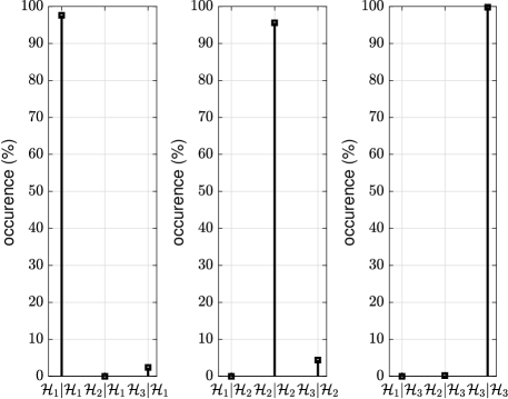
Figure 10: Classification histograms for all the three hypotheses $\mathcal{H}_{1}$, $\mathcal{H}_{2}$, and $\mathcal{H}_{3}$ assuming $M=K=16$ and SINR$=20$ dB.

Note that the Hausdorff metric decreases as the SINR increases up to $15$ dB and then it takes on a constant value equal to $n_{g}=0.4$. Remarkably, the RMS number of missed jammers is close to zero regardless of the SINR, since it depends on the JNR. Finally, Figure 10 contains the classification histograms assuming SINR$=20$ dB. More precisely, each subplot presents the probabilities $P(\mbox{$\mathcal{H}$}_{i}|\mbox{$\mathcal{H}$}_{k})$ as the percentages of declaring $\mbox{$\mathcal{H}$}_{i}$, $i=1,2,3$, when $\mbox{$\mathcal{H}$}_{k}$, $k=1,2,3$, is in force. The histograms highlight that the probability of correct classification, namely of deciding for $\mbox{$\mathcal{H}$}_{i}$ when the latter holds, is close to $1$ at least for the considered parameter setting.

Summarizing, the analysis shows that the SLIM-based detector is very versatile, since it can operates in the presence of NLJ and/or CJs. More importantly, it can ensure excellent signal classification performances allowing for the discrimination between the echoes backscattered from a target and coherent signals emitted by hostile platforms.

V Conclusions

In this paper, we have devised adaptive detection architectures with signal-processing-related ECCM capabilities against the attack of NLJs and/or CJs from the antenna sidelobes. We have analyzed two operating scenarios which differ for the presence of an unknown number of CJs assuming that two independent sets of training samples are available for estimation purposes. Next, we have devised novel signal processing procedures to estimate the ICM capable of providing reliable estimates even in the presence of a low volume of secondary data. Moreover, such estimation procedures work without knowing the actual number of NLJs. In the case where CJs are present, we have conceived a multistage architecture which leverages the hidden sparse nature of the data model to detect structured signals backscattered from a target or generated by CJs. To this end, we have borrowed the SLIM paradigm proposed in [39]. The performance analyses has highlighted that the newly proposed detection architectures exhibit satisfactory performances and, more important, the SLIM-based detector with its classification capabilities can act as an improved SLB, since, in the case where a target and CJs are simultaneously present, it does not blank the possible detection.

Future research tracks might encompass the design of detection architectures for range-spread targets based upon compressive sensing algorithms.

VI ACKNOWLEDGMENTS

This work was partially supported by the National Natural Science Foundation of China under Grant No. 61571434, and Chinese academy of sciences president’s international fellowship initiative under Grant No. 2018VTB0006.

Appendix A MLE of $\mbox{\boldmath{$M$}}_{2}$ for known $r$

In this Appendix, we provide the derivation of (7). To this end, compute the logarithm of $\mbox{$\mathcal{L}$}_{R}(\sigma^{2},\mbox{\boldmath{$M$}}_{nj})$ and recast it by means of the eigendecompositions of $\mbox{\boldmath{$M$}}_{2}$ and $\mbox{\boldmath{$R$}}\mbox{\boldmath{$R$}}^{\dagger}$ as

$$\ln\mbox{$\mathcal{L}$}(\sigma^{2},\mbox{\boldmath{$M$}}_{nj}) =-MN\ln\pi-M\left\{\sum_{i=1}^{r}\ln(\sigma^{2}+\lambda_{nj,i})+(N-r)\ln\sigma^{2}\right\}$$

$$-\mathrm{tr}\left[(\sigma^{2}\textbf{I}+\mbox{\boldmath{$\Lambda$}}_{nj})^{-1}\mbox{\boldmath{$U$}}^{{\dagger}}\mbox{\boldmath{$U$}}_{S1}\mbox{\boldmath{$\Lambda$}}_{S1}\mbox{\boldmath{$U$}}_{S1}^{{\dagger}}\mbox{\boldmath{$U$}}\right]$$

$$=h(\sigma^{2},\mbox{\boldmath{$\Lambda$}}_{j},\mbox{\boldmath{$U$}}),$$ (38)

where

• $\mbox{\boldmath{$\Lambda$}}_{nj}\in{\mathds{R}}^{N\times N}$ is a diagonal matrix whose nonzero entries are the eigenvalues of $\mbox{\boldmath{$M$}}_{nj}$ with $\lambda_{nj,1}\geq\lambda_{nj,2}\geq...\geq\lambda_{nj,r}>0$ and $\mbox{\boldmath{$U$}}\in{\mathds{C}}^{N\times N}$ is the unitary matrix of the corresponding eigenvectors;

• $\mbox{\boldmath{$\Lambda$}}_{S1}\in{\mathds{R}}^{N\times N}$ is a diagonal matrix whose nonzero entries are the eigenvalues of $\mbox{\boldmath{$R$}}\mbox{\boldmath{$R$}}^{\dagger}$, denoted by $\gamma_{1,1}\geq\gamma_{1,2}\geq...\geq\gamma_{1,N}\geq 0$, and $\mbox{\boldmath{$U$}}_{S1}\in{\mathds{C}}^{N\times N}$ contains the corresponding eigenvectors.

Thus, the maximization of $\ln\mbox{$\mathcal{L}$}(\sigma^{2},\mbox{\boldmath{$M$}}_{nj})$ with respect to $\mbox{\boldmath{$M$}}_{2}$ is equivalent to

$$\underset{\sigma^{2},\mbox{\boldmath{$\Lambda$}}_{j},\mbox{\boldmath{$U$}}}{\max}h(\sigma^{2},\mbox{\boldmath{$\Lambda$}}_{j},\mbox{\boldmath{$U$}}).$$ (39)

Now, the optimization with respect to $U$ can be accomplished exploiting Theorem 1 [44], we obtain that

$$\max\limits_{\mbox{\boldmath{$U$}}}\mathrm{tr}\left[(\sigma^{2}\textbf{I}+\mbox{\boldmath{$\Lambda$}}_{j})^{-1}\mbox{\boldmath{$U$}}^{{\dagger}}\mbox{\boldmath{$U$}}_{S1}\mbox{\boldmath{$\Lambda$}}_{S1}\mbox{\boldmath{$U$}}_{S1}^{{\dagger}}\mbox{\boldmath{$U$}}\right] =\max\limits_{\mbox{\boldmath{$W$}}_{1}}\mathrm{tr}[(\sigma^{2}\textbf{I}+\mbox{\boldmath{$\Lambda$}}_{j})^{-1}\mbox{\boldmath{$W$}}_{1}\mbox{\boldmath{$\Lambda$}}_{S1}\mbox{\boldmath{$W$}}_{1}^{{\dagger}}]$$

$$=\mathrm{tr}[(\sigma^{2}\textbf{I}+\mbox{\boldmath{$\Lambda$}}_{j})^{-1}\mbox{\boldmath{$\Lambda$}}_{S1}],$$ (40)

where $\mbox{\boldmath{$W$}}_{1}=\mbox{\boldmath{$U$}}^{{\dagger}}\mbox{\boldmath{$U$}}_{S1}$. It is possible to show that optimization with respect to $\mbox{\boldmath{$W$}}_{1}$ leads to $\mbox{\boldmath{$W$}}_{1}=\mbox{\boldmath{$I$}}e^{j\theta_{1}}$ for arbitrary $\theta_{1}\in[0,2\pi]$. Thus, choosing for simplicity $\theta_{1}=0$, an MLE of $U$ can be recast as $\widehat{\mbox{\boldmath{$U$}}}=\mbox{\boldmath{$U$}}_{S1}$. As a consequence, problem (39) becomes

$$\underset{\sigma^{2},\mbox{\boldmath{$\Lambda$}}_{j}}{\max}g(\sigma^{2},\mbox{\boldmath{$\Lambda$}}_{j}),$$ (41)

where

$$g(\sigma^{2},\mbox{\boldmath{$\Lambda$}}_{j})=-MN\ln\pi-M\left\{\sum_{i=1}^{r}\ln(\sigma^{2}+\lambda_{j,i})+(N-r)\ln\sigma^{2}\right\}-\sum_{i=1}^{r}\frac{\gamma_{1,i}}{\sigma^{2}+\lambda_{j,i}}-\frac{1}{\sigma^{2}}\sum_{i=r+1}^{N}\gamma_{1,i}.$$ (42)

To estimate the remaining parameters, let us set to zero the gradient of $g(\sigma^{2},\mbox{\boldmath{$\Lambda$}}_{j})$. Then, the resulting estimates are given by

$$\widehat{\sigma}^{2}=\frac{1}{M(N-r)}\sum\limits_{i=r+1}^{N}\gamma_{1,i}\quad\mbox{and}\quad\widehat{\lambda}_{j,i}+\widehat{\sigma}^{2}=\frac{\gamma_{1,i}}{M},\quad i=1,...,r.$$ (43)

Finally, the MLE of $\widehat{\mbox{\boldmath{$M$}}}_{2}$ is

$$\widehat{\mbox{\boldmath{$M$}}}_{2}=\mbox{\boldmath{$U$}}_{S1}(\widehat{\sigma}^{2}\mbox{\boldmath{$I$}}+\widehat{\mbox{\boldmath{$\Lambda$}}}_{j})\mbox{\boldmath{$U$}}_{S1}^{{\dagger}},$$ (44)

where $\widehat{\sigma}^{2}\mbox{\boldmath{$I$}}+\widehat{\mbox{\boldmath{$\Lambda$}}}_{j}=\textbf{diag}\left\{\frac{\gamma_{1,1}}{M},\ldots,\frac{\gamma_{1,r}}{M},\frac{1}{M(N-r)}\sum_{i=r+1}^{N}\gamma_{1,i},\ldots,\frac{1}{M(N-r)}\sum_{i=r+1}^{N}\gamma_{1,i}\right\}$.

Appendix B MLE of $\mbox{\boldmath{$M$}}_{c}$ for known $\mbox{\boldmath{$M$}}_{2}$

Assume that $\mbox{\boldmath{$M$}}_{2}$ is known and consider the following maximization problem

$$\max_{\mbox{\boldmath{$M$}}_{c}}\mbox{$\mathcal{L}$}_{Z}(\mbox{\boldmath{$M$}}_{c}),$$ (45)

where $\mbox{$\mathcal{L}$}_{Z}(\mbox{\boldmath{$M$}}_{c})$ is defined by (8). To solve (45), let us recast the logarithm of $\mbox{$\mathcal{L}$}_{Z}(\mbox{\boldmath{$M$}}_{c})$ as

$$-KN\ln\pi-K\ln\det(\mbox{\boldmath{$M$}}_{2})-K\ln\det(\mbox{\boldmath{$I$}}+\mbox{\boldmath{$M$}}_{2}^{-\frac{1}{2}}\mbox{\boldmath{$M$}}_{c}\mbox{\boldmath{$M$}}_{2}^{-\frac{1}{2}})$$

$$-\mathrm{tr}\left[(\mbox{\boldmath{$I$}}+\mbox{\boldmath{$M$}}_{2}^{-\frac{1}{2}}\mbox{\boldmath{$M$}}_{c}\mbox{\boldmath{$M$}}_{2}^{-\frac{1}{2}})^{-1}\mbox{\boldmath{$M$}}_{2}^{-\frac{1}{2}}\mbox{\boldmath{$Z$}}\mbox{\boldmath{$Z$}}^{\dagger}\mbox{\boldmath{$M$}}_{2}^{-\frac{1}{2}}\right]$$

$$=-KN\ln\pi-K\ln\det(\mbox{\boldmath{$M$}}_{2})-K\ln\det(\mbox{\boldmath{$I$}}+\mbox{\boldmath{$\Omega$}}_{c})-\mathrm{tr}\left[(\mbox{\boldmath{$I$}}+\mbox{\boldmath{$\Omega$}}_{c})^{-1}\mbox{\boldmath{$V$}}^{{\dagger}}\mbox{\boldmath{$U$}}_{S2}\mbox{\boldmath{$\Lambda$}}_{S2}\mbox{\boldmath{$U$}}_{S2}^{{\dagger}}\mbox{\boldmath{$V$}}\right]$$

$$=\mbox{$\mathcal{L}$}_{Z}(\mbox{\boldmath{$V$}},\mbox{\boldmath{$\Omega$}}_{c}),$$ (46)

where the last equality is due to the eigendecomposition of $\mbox{\boldmath{$M$}}_{2}^{-\frac{1}{2}}\mbox{\boldmath{$M$}}_{c}\mbox{\boldmath{$M$}}_{2}^{-\frac{1}{2}}$ and $\mbox{\boldmath{$Z$}}\mbox{\boldmath{$Z$}}^{\dagger}$. In fact, in (B), $\mbox{\boldmath{$\Lambda$}}_{S2}\in{\mathds{R}}^{N\times N}$ is a diagonal matrix whose nonzero entries are the eigenvalues of $\mbox{\boldmath{$M$}}_{2}^{-\frac{1}{2}}\mbox{\boldmath{$Z$}}\mbox{\boldmath{$Z$}}^{\dagger}\mbox{\boldmath{$M$}}_{2}^{-\frac{1}{2}}$ denoted by $\gamma_{2,1}\geq...\geq\gamma_{2,N}\geq 0$ with $\mbox{\boldmath{$U$}}_{S2}\in{\mathds{C}}^{N\times N}$ the unitary matrix of the corresponding eigenvectors and $\mbox{\boldmath{$\Omega$}}_{c}\in{\mathds{R}}^{N\times N}$ is the diagonal matrix containing the eigenvalues of $\mbox{\boldmath{$M$}}_{2}^{-\frac{1}{2}}\mbox{\boldmath{$M$}}_{c}\mbox{\boldmath{$M$}}_{2}^{-\frac{1}{2}}$ denoted by $\lambda_{c,1}\geq...\geq\lambda_{c,N}>0$ with $\mbox{\boldmath{$V$}}\in{\mathds{C}}^{N\times N}$ the unitary matrix of the corresponding eigenvectors. It follows that problem (45) becomes

$$\max_{\mbox{\boldmath{$V$}},\mbox{\boldmath{$\Omega$}}_{c}}\mbox{$\mathcal{L}$}_{Z}(\mbox{\boldmath{$V$}},\mbox{\boldmath{$\Omega$}}_{c}).$$ (47)

The optimization with respect to $V$ can be accomplished adopting the same line of reasoning as for $\mbox{\boldmath{$W$}}_{1}$ in Appendix A, namely

$$\max\limits_{\mbox{\boldmath{$V$}}}\mathrm{tr}\left[(\mbox{\boldmath{$I$}}+\mbox{\boldmath{$\Omega$}}_{c})^{-1}\mbox{\boldmath{$V$}}^{{\dagger}}\mbox{\boldmath{$U$}}_{S2}\mbox{\boldmath{$\Lambda$}}_{S2}\mbox{\boldmath{$U$}}_{S2}^{{\dagger}}\mbox{\boldmath{$V$}}\right] =\max\limits_{\mbox{\boldmath{$W$}}_{2}}\mathrm{tr}[(\mbox{\boldmath{$I$}}+\mbox{\boldmath{$\Omega$}}_{c})^{-1}\mbox{\boldmath{$W$}}_{2}\mbox{\boldmath{$\Lambda$}}_{S2}\mbox{\boldmath{$W$}}_{2}^{{\dagger}}]$$

$$=\mathrm{tr}[(\mbox{\boldmath{$I$}}+\mbox{\boldmath{$\Omega$}}_{c})^{-1}\mbox{\boldmath{$\Lambda$}}_{S2}],$$ (48)

where $\mbox{\boldmath{$W$}}_{2}=\mbox{\boldmath{$V$}}^{{\dagger}}\mbox{\boldmath{$U$}}_{S2}$ and the last equality comes from the fact that $\widehat{\mbox{\boldmath{$W$}}}_{2}=\mbox{\boldmath{$I$}}e^{j\theta_{2}}$ with $\theta_{2}\in[0,2\pi]$ arbitrary. As a result, an estimate of $V$ is $\widehat{\mbox{\boldmath{$V$}}}=\mbox{\boldmath{$U$}}_{S2}$.

The final step consists in solving

$$\max_{\mbox{\boldmath{$\Omega$}}_{c}}\bar{g}(\mbox{\boldmath{$\Omega$}}_{c}),$$ (49)

where

$$\bar{g}(\mbox{\boldmath{$\Omega$}}_{c})=-K\sum_{i=1}^{N}\ln(1+\lambda_{c,i})-\sum_{i=1}^{N}\frac{\gamma_{2,i}}{1+\lambda_{c,i}}.$$ (50)

Thus, setting to zero the gradient of $\bar{g}(\mbox{\boldmath{$\Omega$}}_{c})$, we obtain

$$\widehat{\lambda}_{c,i}=\max\left\{\frac{\gamma_{2,i}}{K}-1,0\right\},\quad i=1,\ldots,N.$$ (51)

Gathering the above results, the MLE of $\mbox{\boldmath{$M$}}_{c}$ for known $\mbox{\boldmath{$M$}}_{2}$ is

$$\widehat{\mbox{\boldmath{$M$}}}_{c}[\mbox{\boldmath{$M$}}_{2}]=\mbox{\boldmath{$M$}}_{2}^{\frac{1}{2}}\mbox{\boldmath{$U$}}_{S2}\widehat{\mbox{\boldmath{$\Omega$}}}_{c}\mbox{\boldmath{$U$}}_{S2}^{{\dagger}}\mbox{\boldmath{$M$}}_{2}^{\frac{1}{2}},$$ (52)

where $\widehat{\mbox{\boldmath{$\Omega$}}}_{c}=\textbf{diag}\left\{\widehat{\lambda}_{c,1},\ldots,\widehat{\lambda}_{c,N}\right\}$.

Table I: List of Acronyms

Acronyms
AIC	Akaike Information Criterion
AOA	Angle of Arrival
AMF	Adaptive Matched Filter
BIC	Bayesian Information Criterion
CJ	Coherent Jammer
CNR	Clutter-to-Noise Ratio
CUT	Cell Under Test
DT	Double Trained
ECCM	Electronic Counter-countermeasure
ECM	Electronic Countermeasure
GIC	Generalized Information Criterion
GLRT	Generalized Likelihood Ratio Test
ICM	Interference Covariance Matrix
IDT	Improved Double Trained
JNR	Jammer-to-Noise Ratio
LRT	Likelihood Ratio Test
MLA	Maximum Likelihood Approach
MLE	Maximum Likelihood Estimate
NLJ	Noise Like Jammer
MOS	Model Order Selection
RMS	Root Mean Square
SINR	Signal-to-Interference plus Noise Ratio
SLB	Sidelobe Blanker
SLC	Sidelobe Canceler
SLIM	Sparse Learning via Iterative Minimization

References

- [1] M. A. Richards, J. A. Scheer, and W. A. Holm, Principles of Modern Radar: Basic Principles. Raleigh, NC: Scitech Publishing, 2010.
- [2] A. Farina, Antenna-Based Signal Processing Techniques for Radar Systems. Boston, MA: Artech House, 1992.
- [3] D. Adamy, EW101: A First Course in Electronic Warfare. Norwood, MA: Artech House, 2001.
- [4] W. L. Melvin and J. A. Scheer, Principles of Modern Radar: Advanced Techniques. Edison, NJ: Scitech Publishing, 2013.
- [5] E. J. Kelly, “An adaptive detection algorithm,” IEEE Transactions on Aerospace and Electronic Systems, vol. 22, no. 2, pp. 115–127, 1986.
- [6] F. C. Robey, D. R. Fuhrmann, E. J. Kelly, and R. Nitzberg, “A CFAR adaptive matched filter detector,” IEEE Transactions on Aerospace and Electronic Systems, vol. 28, no. 1, pp. 208–216, 1992.
- [7] F. Gini and A. Farina, “Vector subspace detection in compound-Gaussian clutter Part I: Survey and new results,” IEEE Transactions on Aerospace and Electronic Systems, vol. 38, no. 4, pp. 1295–1311, 2002.
- [8] A. De Maio, “Rao test for adaptive detection in Gaussian interference with unknown covariance matrix,” IEEE Transactions on Signal Processing, vol. 55, no. 7, pp. 3577–3584, 2007.
- [9] A. De Maio, S. M. Kay, and A. Farina, “On the invariance, coincidence, and statistical equivalence of the glrt, rao test, and wald test,” IEEE Transactions on Signal Processing, vol. 58, no. 4, pp. 1967–1979, 2010.
- [10] D. Orlando and G. Ricci, “A rao test with enhanced selectivity properties in homogeneous scenarios,” IEEE Transactions on Signal Processing, vol. 58, no. 10, pp. 5385–5390, 2010.
- [11] W. Liu, W. Xie, and Y. Wang, “Rao and wald tests for distributed targets detection with unknown signal steering,” IEEE Signal Processing Letters, vol. 20, no. 11, pp. 1086–1089, 2013.
- [12] N. Li, G. Cui, L. Kong, and X. Yang, “Rao and wald tests design of multiple-input multiple-output radar in compound-gaussian clutter,” IET Radar, Sonar & Navigation, vol. 6, no. 8, pp. 729–738, 2012.
- [13] F. Bandiera, D. Orlando, and G. Ricci, Advanced Radar Detection Schemes Under Mismatched Signal Models. San Rafael, US: Synthesis Lectures on Signal Processing No. 8, Morgan & Claypool Publishers, 2009.
- [14] P. Addabbo, A. Aubry, A. De Maio, L. Pallotta, and S. L. Ullo, “HRR profile estimation using SLIM,” IET Radar, Sonar Navigation, vol. 13, no. 4, pp. 512–521, 2019.
- [15] J. Liu, W. Liu, B. Chen, H. Liu, H. Li, and C. Hao, “Modified rao test for multichannel adaptive signal detection,” IEEE Transactions on Signal Processing, vol. 64, no. 3, pp. 714–725, 2016.
- [16] J. Liu, H. Li, and B. Himed, “Persymmetric adaptive target detection with distributed MIMO radar,” IEEE Transactions on Aerospace and Electronic Systems, vol. 51, no. 1, pp. 372–382, 2015.
- [17] J. Liu, G. Cui, H. Li, and B. Himed, “On the performance of a persymmetric adaptive matched filter,” IEEE Transactions on Aerospace and Electronic Systems, vol. 51, no. 4, pp. 2605–2614, 2015.
- [18] C. Hao, S. Gazor, G. Foglia, B. Liu, and C. Hou, “Persymmetric adaptive detection and range estimation of a small target,” IEEE Transactions on Aerospace and Electronic Systems, vol. 51, no. 4, pp. 2590–2604, 2015.
- [19] J. Liu, H. Li, and B. Himed, “Persymmetric adaptive target detection with distributed mimo radar,” IEEE Transactions on Aerospace and Electronic Systems, vol. 51, no. 1, pp. 372–382, 2015.
- [20] J. Liu, G. Cui, H. Li, and B. Himed, “On the performance of a persymmetric adaptive matched filter,” IEEE Transactions on Aerospace and Electronic Systems, vol. 51, no. 4, pp. 2605–2614, 2015.
- [21] A. De Maio and D. Orlando, “An invariant approach to adaptive radar detection under covariance persymmetry,” IEEE Transactions on Signal Processing, vol. 63, no. 5, pp. 1297–1309, 2015.
- [22] P. Wang, Z. Sahinoglu, M. Pun, and H. Li, “Persymmetric Parametric Adaptive Matched Filter for Multichannel Adaptive Signal Detection,” IEEE Transactions on Signal Processing, vol. 60, no. 6, pp. 3322–3328, 2012.
- [23] L. Cai and H. Wang, “A persymmetric multiband glr algorithm,” IEEE Transactions on Aerospace and Electronic Systems, vol. 28, no. 3, pp. 806–816, 1992.
- [24] A. De Maio, D. Orlando, C. Hao, and G. Foglia, “Adaptive detection of point-like targets in spectrally symmetric interference,” IEEE Transactions on Signal Processing, vol. 64, no. 12, pp. 3207–3220, 2016.
- [25] C. Hao, D. Orlando, G. Foglia, and G. Giunta, “Knowledge-based adaptive detection: Joint exploitation of clutter and system symmetry properties,” IEEE Signal Processing Letters, vol. 23, no. 10, pp. 1489–1493, 2016.
- [26] G. Foglia, C. Hao, A. Farina, G. Giunta, D. Orlando, and C. Hou, “Adaptive detection of point-like targets in partially homogeneous clutter with symmetric spectrum,” IEEE Transactions on Aerospace and Electronic Systems, vol. 53, no. 4, pp. 2110–2119, 2017.
- [27] S. U. Pillai, Y. L. Kim, and J. R. Guerci, “Generalized forward/backward subaperture smoothing techniques for sample starved STAP,” IEEE Transactions on Signal Processing, vol. 48, no. 12, pp. 3569–3574, 2000.
- [28] G. Pailloux, P. Forster, J. P. Ovarlez, and F. Pascal, “Persymmetric adaptive radar detectors,” IEEE Transactions on Aerospace and Electronic Systems, vol. 47, no. 4, pp. 2376–2390, 2011.
- [29] A. Farina, “Eccm techniques,” in Radar Handbook, M. I. Skolnik, Ed. McGraw-Hill, 2008, ch. 24.
- [30] M. Greco, F. Gini, A. Farina, and V. Ravenni, “Effect of phase and range gate pull-off delay quantisation on jammer signal,” IEE Proceedings - Radar, Sonar and Navigation, vol. 153, no. 5, pp. 454–459, 2006.
- [31] A. Farina and F. Gini, “Calculation of blanking probability for the sidelobe blanking for two interference statistical models,” IEEE Signal Processing Letters, vol. 5, no. 4, pp. 98–100, 1998.
- [32] A. De Maio, A. Farina, and F. Gini, “Performance analysis of the sidelobe blanking system for two fluctuating jammer models,” IEEE Transactions on Aerospace and Electronic Systems, vol. 41, no. 3, pp. 1082–1091, 2005.
- [33] G. Cui, A. De Maio, M. Piezzo, and A. Farina, “Sidelobe blanking with generalized swerling-chi fluctuation models,” IEEE Transactions on Aerospace and Electronic Systems, vol. 49, no. 2, pp. 982–1005, 2013.
- [34] A. Farina, “Single sidelobe canceller: Theory and evaluation,” IEEE Transactions on Aerospace and Electronic Systems, vol. 13, no. 6, pp. 690–699, 1977.
- [35] E. J. Hendon and I. S. Reed, “A new CFAR sidelobe canceler algorithm for radar,” IEEE Transactions on Aerospace and Electronic Systems, vol. 26, no. 5, pp. 792–803, 1990.
- [36] A. Farina, L. Timmoneri, and R. Tosini, “Cascading SLB and SLC devices,” Signal Processing, vol. 45, no. 2, pp. 261 – 266, 1995.
- [37] V. Carotenuto, A. De Maio, D. Orlando, and L. Pallotta, “Adaptive radar detection using two sets of training data,” IEEE Transactions on Signal Processing, vol. 66, no. 7, pp. 1791–1801, 2018.
- [38] P. Stoica and Y. Selen, “Model-order selection: A review of information criterion rules,” IEEE Signal Processing Magazine, vol. 21, no. 4, pp. 36–47, 2004.
- [39] X. Tan, W. Roberts, J. Li, and P. Stoica, “Sparse learning via iterative minimization with application to mimo radar imaging,” IEEE Transactions on Signal Processing, vol. 59, no. 3, pp. 1088–1101, 2011.
- [40] R. A. Horn and C. R. Johnson, Matrix Analysis, C. U. Press, Ed., 1985.
- [41] L. Van Brunt, Applied ECM. EW Engineering, 1982, vol. 2.
- [42] H. L. Van Trees, Optimum Array Processing (Detection, Estimation, and Modulation Theory, Part IV). John Wiley & Sons, 2002.
- [43] D. Schuhmacher, B. Vo, and B. Vo, “A consistent metric for performance evaluation of multi-object filters,” IEEE Transactions on Signal Processing, vol. 56, no. 8, pp. 3447–3457, 2008.
- [44] L. Mirsky, “On the trace of matrix products,” Mathematische Nachrichten, vol. 20, pp. 171–174, 1959.