Turbulent kinetic energy production and flow structures in flows past smooth and rough walls

Abstract

Data available in literature from direct numerical simulations of two-dimensional turbulent channels by Lee & Moser (2015), Bernardini et al. (2014), Yamamoto & Tsuji (2018) and Orlandi et al. (2015) in a large range of Reynolds number have been used to find that $S^{*}$ the ratio between the eddy turnover time ($q^{2}/\epsilon$) and the time scale of the mean deformation ($1/S$), scales very well with the Reynolds number in the near-wall region. The good scaling is due to the eddy turnover time, although the turbulent kinetic energy and the rate of isotropic dissipation show a Reynolds dependence near the wall. $S^{*}$ is linked to the flow structures, as well as $-{\langle Q\rangle}=\langle{s_{ij}s_{ji}}\rangle-\langle{\omega_{i}\omega_{i}/2}\rangle$ and also this quantity presents a good scaling. It has been found that the maximum of turbulent kinetic energy production $P_{k}$ occurs in the layer with $-{\langle Q\rangle}\approx 0$ that is where the unstable sheet-like structures roll-up to become rods. The decomposition of $P_{k}$ in the contribution of elongational and compressive strain demonstrates that the two contribution present a good scaling. The perfect scaling however holds when the near-wall and the outer structures are separated. The same statistics have been evaluated by direct simulations of turbulent channels with different type of corrugations on both walls. The flow physics in the layer near the plane of the crests is strongly linked to the shape of the surface and it has been demonstrated that the $u_{2}$ (normal to the wall) fluctuations are responsible for the modification of the flow structures, for the increase of the resistance and of the turbulent kinetic energy production. These simulations at intermediate Reynolds number indicated that in the outer region the Townsend similarity hypothesis holds.

1 Introduction

Turbulent flows near smooth walls are characterised by flow structures of different size and intensity that have been observed and described by very impressive flow visualizations by Kline et al. (1967). In laboratory experiments it is rather difficult to measure any quantity, therefore the deep understanding of the flow complexity can not be achieved. The evolution of hardware and software necessary for the solution of the non-linear Navier-Stokes equations allowed to evaluate any flow variable and to increase the knowledge of the physics of turbulent flows. The simulations were performed for a large amount of turbulent flows and in particular for wall bounded flows such as boundary layers, circular pipes and two-dimensional channels. In this paper the study is focused on flows in two-dimensional channels past smooth and corrugated walls. The first Direct Numerical Simulation (DNS) of a two-dimensional channel by Moin & Kim (1982) can be considered a scientific revolution, in fact after this publication a large number of scholars and even some experimentalist directed their research work on the use of numerical methods to produce and analyse turbulent data to understand the complex physics of wall bounded turbulent flows. The direct comparison between numerical and laboratory flow visualizations in Moin & Kim (1997) can be considered a proof that the Navier-Stokes equations are the valid model to describe the evolution of turbulent flows. After that simulation at low Reynolds number ($R_{\tau}=u_{\tau}h/\nu=180$ with $u_{\tau}$ the friction velocity $h$ half channel height and $\nu$ the kinematic viscosity) there was a large effort to increase the Reynolds number. The relevant efforts were done, among several groups by Jimenez & Hoyas (2008) up to $R_{\tau}=2000$ by Bernardini et al. (2014) up to $R_{\tau}=4000$, by Lee & Moser (2015) up to $R_{\tau}=5200$ and recently by Yamamoto & Tsuji (2018) up to $R_{\tau}=8000$. Some of the statistics in these papers together with others at low Reynolds number in Orlandi et al. (2015) are used in this study to calculate quantities linked to the flow structures and therefore to investigate the dependence on the Reynolds number. Namely these are the shear rate parameter $S^{*}=Sq^{2}/\epsilon$ defined as the ratio between the eddy turnover time $q^{2}/\epsilon$ ( $q^{2}$ is twice the turbulent kinetic energy and $\epsilon$ is the isotropic dissipation rate) and the time scale of the mean deformation $1/S=2/{{dU}\over{dx_{2}}}$ ($U$ stands for $\langle u_{1}\rangle$). The shear parameter was used by Lee et al. (1990) to prove that the elongated wall structures, observed by Kline et al. (1967), were not generated by the presence of the solid wall, instead by the mean shear rate $S$ if it was greater than a threshold value. As it was shown by Orlandi et al. (2015) the profiles of the shear parameter do not largely vary with the Reynolds number in presence of smooth walls. This conclusion is a first evidence that the laboratory experiments have limitations to explain the complex physics of turbulent flows due to the impossibility to measure $\epsilon$ in the whole channel and in particular near the wall. The profiles of $\epsilon^{+}$ as well as those of $q^{2+}$ (the superscript $+$ indicates wall units) are Reynolds dependent. In this paper it is shown that, near the walls, the eddy turnover time as well as the mean shear in wall units do not depend on the Reynolds number, therefore the shear parameters can be considered a fundamental quantity to characterise the energetic scales near smooth walls.

The production of turbulent energy $P_{k}=-\langle u_{1}u_{2}\rangle{{dU}\over{dx_{2}}}$ (small letters indicate fluctuations) is strictly linked to $S$. When the near-wall and the outer turbulent structures are separated the production does not depend on the Reynolds number. At low $Re$, on the other hand, the maximum of $P_{k}^{+}$, from zero for the laminar regime jumps to a value $0.15$ at the transitional Reynolds number. Hence it gradually grows with $R_{\tau}$ to saturate at $500<R_{\tau}$ at a value equal to $0.25$. Due to the key role of $S$ the one-dimensional statistics profiles can be projected on the eigenvectors of the tensor $S_{ij}$. In this frame there is a negative compressive $S_{\alpha}$ and a positive extensional $S_{\gamma}$ strain. The turbulent kinetic production in this local frame is $P_{k}=-(P_{\alpha}+P_{\gamma})$ with the terms $P_{\alpha}=R_{\alpha\alpha į}S_{\alpha}$ and $P_{\gamma}=R_{\gamma\gamma}S_{\gamma}$ greater than $P_{k}$. Their profiles allow to understand that the compressive strain generates more kinetic energy than that destroyed by extensional one. The projection of the statistics along the eigenvectors of the tensor $S_{ij}$ shows a decrease on the anisotropy of the velocity and vorticity correlation and can give insights on turbulence closures. The stresses in the spanwise direction, as it should be expected, do not change in this new reference frame with $S_{\beta}=0$.

The production of turbulent kinetic energy can also be expressed in a different way. (Orlandi (2000) at Pg.211) with $P_{k}=P_{T}+P_{C}$. This expression is derived by the Navier-Stokes equation in rotational form. $P_{C}={{\partial U\langle u_{1}u_{2}\rangle}\over{\partial x_{2}}}$ is related to the action of the large eddies advecting the turbulence across the channel. $P_{T}=U(\langle u_{3}\omega_{2}\rangle-\langle u_{2}\omega_{3}\rangle)$ is linked to the energy transfer from large to small eddies.

Orlandi (2013) in turbulent wall bounded flows emphasised the role of the wall-normal Reynolds stress and therefore the statistics linked to the $u_{2}$ velocity fluctuations and in particular those connected to the flow structures should be analysed. This stress received little attention, in particular because of the difficulty to get accurate measurements near the walls. It is worth to recall that only this stress appears in the mean momentum equation and it is balanced by the mean pressure $\langle{p}\rangle$. As it was discussed in that paper as well as by Tsinober (2009) at Pg.162 the topology of flow structures can be described by $-Q=s_{ij}s_{ji}-\omega_{i}\omega_{i}/2$, where regions with $Q<0$ are sheet-dominated and regions with $Q>0$ are associated with tube-like structures. In homogeneous turbulence ${\langle Q\rangle}=0$ In non-homogeneous turbulent flows ${{d^{2}\langle u_{2}^{2}\rangle}\over{dx_{2}^{2}}}=-{\langle Q\rangle}=\langle{s_{ij}s_{ji}}\rangle-\langle{\omega_{i}\omega_{i}/2}\rangle$ accounts for the disequilibrium between $\langle{s_{ij}s_{ji}}\rangle$ and $\langle{\omega_{i}\omega_{i}/2}\rangle$. Hence the term ${{d^{2}\langle u_{2}^{2}\rangle}\over{dx_{2}^{2}}}$ determines whether in a region there is a prevalence of sheet-like or rod-like structures. The former are inherently unsteady, and roll-up producing turbulent kinetic energy. A detailed study on the difference between the shape of ribbon- and rod-like structures requires appropriate eduction schemes as those described by Pirozzoli et al. (2010). The profiles of the turbulent kinetic energy production, in their different form, together with the profiles of ${{d^{2}\langle u_{2}^{2}\rangle}\over{dx_{2}^{2}}}$ shows that the maximum production occurs in the layer separating sheet- and tubular-dominated regions. One of the goals in performing DNS of two-dimensional turbulent channels at high Reynolds numbers was and still is to investigate the Reynolds number dependence on the statistics. The aim of the present study is to see whether the above mentioned statistics , in wall units, related to the flow structures present a minor or almost a complete Reynolds number independence in the near-wall region.

A rediscovered and improved version of the old Immersed Boundary Technique used by Peskin (1972) for bio-inspired flows was developed by Orlandi & Leonardi (2006) to perform DNS of turbulent flows past rough walls. The method was validated in several papers and the convincing proof of its accuracy was reported by Burattini et al. (2008) by comparing the statistics derived by the numerical experiments with those measured in laboratory, The experiments were designed with the aim to show that true DNS can be accomplished by the immersed boundary technique inserted in a second order finite difference method. In this paper the corrugations are located in both walls and the solutions are obtained at intermediate values of the $Re$ number, namely approximately at $R_{\tau}=200$ in presence of smooth walls. Longitudinal transverse and three-dimensional elements are considered producing a drag increase with the exception of a geometry similar to that investigated by Choi et al. (1993) producing drag reduction. Near rough walls the flow structures change leading to different profiles of the turbulent statistics above mentioned as it is shown in this paper.

2 Results

2.1 Smooth wall

In this section the data in the web of the DNS at high Reynolds numbers by Bernardini et al. (2014), by Lee & Moser (2015) and by Yamamoto & Tsuji (2018) are used to investigate the eventual Reynolds independence of the shear parameter and their components. The data at low $Re$ are those used in Orlandi et al. (2015). The shear parameter $S^{*}$ is one of the statistics linked to certain kind of flow structures, in fact if $S^{*}$ is greater than a threshold value, approximately $5$, very elongated anisotropic longitudinal structures form. It has been observed that in the near-wall region $S^{*}$ is high and in the outer is small, consequently the flow structures are more intense near the wall than those in the outer region. The profiles of $q^{2+}$ in figure 1a and of $\epsilon^{+}$ in figure 1b show a large $Re$ dependence in the near-wall region, that has been emphasised by plotting the quantities only in the viscous and buffer regions. These two figures show that large variations appear at intermediate $Re$ and that both quantities tend to a limit at high $Re$. Still it has not been established whether a saturation or a logarithmic growth of the maximum of $q^{2+}$ occurs for $Re\rightarrow\infty$ . However, figures 1a seems to infer a saturation. The value of the maximum of $q^{2+}$ at $R_{\tau}=8000$ is twice the value reached at the transitional Reynolds number. At this $Re$ there is no separation between outer and near-wall structures. The peak is located almost at the same distance, in wall units, as that at a $Re$ number hundred times greater. The rate of isotropic energy dissipation in figure 1b shows a large Reynolds number dependence in the region $y^{+}<10$, being this quantity linked to the small scales. As it is discussed later on, for $y^{+}<10$, the full rate of energy dissipation $D_{k}=2\nu\langle u_{i}\nabla^{2}u_{i}\rangle$, in wall units, shows a reduced dependence with the Reynolds number. Since $D_{k}=\nu{{d^{2}\langle q^{2}\rangle}\over{dx^{2}_{2}}}-\epsilon$ it can be concluded that the Reynolds dependence of $\epsilon^{+}$, in the near-wall region, is due to the viscous diffusion of $q^{2+}$. The Reynolds dependence for $y^{+}<10$, at very high $Re$, in the outer region disappears by looking at the profiles of the eddy turnover time, in wall units in figure 1c.

\psfrag{ylab}{\large$q^{2+}$}\psfrag{xlab}{\large$$ }\includegraphics[width=213.39566pt]{fig1_a.eps}

\psfrag{ylab}{\large$q^{2+}$}\psfrag{xlab}{\large$$ }\psfrag{ylab}{\large$\epsilon^{+}$ }\psfrag{xlab}{\large$$ }\includegraphics[width=213.39566pt]{fig1_b.eps}

a)                                                             b) \psfrag{ylab}{\large$q^{2+}$}\psfrag{xlab}{\large$$ }\psfrag{ylab}{\large$\epsilon^{+}$ }\psfrag{xlab}{\large$$ }\psfrag{ylab}{\large$(q^{2}/\epsilon)^{+}$}\psfrag{xlab}{\large$y^{+}$ }\includegraphics[width=213.39566pt]{fig1_c_new.eps} \psfrag{ylab}{\large$q^{2+}$}\psfrag{xlab}{\large$$ }\psfrag{ylab}{\large$\epsilon^{+}$ }\psfrag{xlab}{\large$$ }\psfrag{ylab}{\large$(q^{2}/\epsilon)^{+}$}\psfrag{xlab}{\large$y^{+}$ }\psfrag{ylab}{\large$Sq^{2}/\epsilon$}\psfrag{xlab}{\large$y^{+}$ }\includegraphics[width=213.39566pt]{fig1_d.eps}                                            c)                                                             d) \psfrag{ylab}{\large$q^{2+}$}\psfrag{xlab}{\large$$ }\psfrag{ylab}{\large$\epsilon^{+}$ }\psfrag{xlab}{\large$$ }\psfrag{ylab}{\large$(q^{2}/\epsilon)^{+}$}\psfrag{xlab}{\large$y^{+}$ }\psfrag{ylab}{\large$Sq^{2}/\epsilon$}\psfrag{xlab}{\large$y^{+}$ }\psfrag{ylab}{\large$(q^{2}/D_{k})^{+}$}\psfrag{xlab}{\large$y^{+}$ }\includegraphics[width=213.39566pt]{fig1_e.eps} \psfrag{ylab}{\large$q^{2+}$}\psfrag{xlab}{\large$$ }\psfrag{ylab}{\large$\epsilon^{+}$ }\psfrag{xlab}{\large$$ }\psfrag{ylab}{\large$(q^{2}/\epsilon)^{+}$}\psfrag{xlab}{\large$y^{+}$ }\psfrag{ylab}{\large$Sq^{2}/\epsilon$}\psfrag{xlab}{\large$y^{+}$ }\psfrag{ylab}{\large$(q^{2}/D_{k})^{+}$}\psfrag{xlab}{\large$y^{+}$ }\psfrag{ylab}{\large$$}\psfrag{xlab}{\large$y^{+}$ }\includegraphics[width=213.39566pt]{fig1_f.eps}                                            e)                                                             f)

Figure 1: Profiles in wall units of: a) Turbulent kinetic energy, b) rate of dissipation, c) eddy turnover time evaluated with $\epsilon$ (solid line $2x^{2}$ dashed $10x$), d) shear parameter, e),f) eddy turnover time evaluated with $D_{k}$ (solid line $15x$ dashed $5x$), for channel flows past smooth walls, the data are from the references given in the text. The Reynolds number are in the insets of a); in b), c), d), e), f) the profiles at $R_{\tau}=8000$ could not be evaluated from the Yamamoto & Tsuji (2018) data.

In the near-wall region the eddy turnover time is proportional to $y^{2+}$ instead in the outer region is proportional to $y^{+}$. Figure 1c shows a deviation from the linear behavior higher smaller $Re$ is. In order to appreciate better the variations in the region of transition in the inset some of the profiles are plotted in linear scale. The eddy turnover time based on $D_{k}^{+}$ (figure 1e) instead of on $\epsilon^{+}$ shows a linear increase with $y^{+}$ also near the wall. Therefore it can be stressed that this dimensionless eddy turnover time depicts an universal behavior for the inner and outer structures. These have the same characteristics being generated by the strain $S$, are fast near the wall, and slow in the outer region. The transition between the two similar structures occurs in the region with high growth of turbulent kinetic energy production. To demonstrate the collapse in the near-wall region and the tendency to the saturation in the buffer region figure 1f has been plotted in linear scales and the data at $R_{\tau}=78$ were not considered. At $Re$ numbers close to the transitional value ($R_{\tau}\approx 80$) the two kind of structures are strongly connected and hence the similarity disappears and the flow physics is more complex. In the transitional regime the turbulence could play a large effect in mixing processes or in heat transfer. From the data in figure 2 in Orlandi et al. (2015) it has been evaluated that for $70<R_{\tau}<200$, $K/(hU_{b}^{2})$ ( $K=\int q^{2}dy$ and $U_{b}$ the bulk velocity) decays with $R_{\tau}^{1/3}$ and that for $500<R_{\tau}<5200$ with $R_{\tau}^{1/6}$. Therefore it can be inferred that the effects of Reynolds number are high when the near-wall and the outer structures have the same size, and a strong interconnection. When the near-wall structures are much smaller and far apart from the outer ones the effect of the Reynolds number is reduced. The profiles of $S^{+}$ for $y^{+}<200$ are not given being superimposed each other with the exception of that at $R_{\tau}=78$. Therefore the Reynolds independence of the shear parameter $S^{*}$ in figure 1d is due to the universality of the eddy turnover time in the near-wall region. It can be argued that the similarity in the mean velocity profiles for wall bounded turbulent flows past smooth walls, having well defined boundary conditions, forces the similarity in the eddy turnover time of turbulent flows.

\psfrag{ylab}{\hskip-28.45274pt\large$(10^{2}{{d\langle{u_{2}^{2}}\rangle}\over{dx^{2}_{2}}})^{+}$}\psfrag{xlab}{ $$}\includegraphics[width=213.39566pt]{fig2_a.eps}

\psfrag{ylab}{\hskip-28.45274pt\large$(10^{2}{{d\langle{u_{2}^{2}}\rangle}\over{dx^{2}_{2}}})^{+}$}\psfrag{xlab}{ $$}\psfrag{ylab}{\large$P_{k}^{+}$}\psfrag{xlab}{\large$$ }\includegraphics[width=213.39566pt]{fig2_b.eps}

a)                                                             b) \psfrag{ylab}{\hskip-28.45274pt\large$(10^{2}{{d\langle{u_{2}^{2}}\rangle}\over{dx^{2}_{2}}})^{+}$}\psfrag{xlab}{ $$}\psfrag{ylab}{\large$P_{k}^{+}$}\psfrag{xlab}{\large$$ }\psfrag{ylab}{\large$D_{k}^{+}$}\psfrag{xlab}{\large$y^{+}$ }\includegraphics[width=213.39566pt]{fig2_c.eps} \psfrag{ylab}{\hskip-28.45274pt\large$(10^{2}{{d\langle{u_{2}^{2}}\rangle}\over{dx^{2}_{2}}})^{+}$}\psfrag{xlab}{ $$}\psfrag{ylab}{\large$P_{k}^{+}$}\psfrag{xlab}{\large$$ }\psfrag{ylab}{\large$D_{k}^{+}$}\psfrag{xlab}{\large$y^{+}$ }\psfrag{ylab}{\large$T_{k}^{+}$}\psfrag{xlab}{\large$y^{+}$ }\includegraphics[width=213.39566pt]{fig2_d.eps}                                            c)                                                             d)

Figure 2: Profiles in wall units of: a) ${{d^{2}{\langle u_{2}^{2}\rangle}}\over{dx^{2}_{2}}}$, b) turbulent kinetic energy production, c) full rate of dissipation , d) turbulent diffusion by non-linear terms, the data are from the references given in the text. The Reynolds number are in the insets of a); in c), d) the profiles at $R_{\tau}=8000$ could not be evaluated from the Yamamoto & Tsuji (2018) data.

To understand in more detail the influence of the Reynolds number on the flow structures in the near-wall region it is worth to look at the profiles of ${{d^{2}{\langle u_{2}^{2}\rangle}}\over{dx^{2}_{2}}}=-{\langle Q\rangle}$. As previously mentioned this quantity is null in homogeneous turbulent flows, for $-{\langle Q\rangle}>0$ sheet-like structures prevail on tubular like structures. In the near-wall region the sheets produce and dissipate turbulent kinetic energy. The profiles in wall units of ${{d^{2}{\langle u_{2}^{2}\rangle}}\over{dx^{2}_{2}}}$, $P_{k}$ and $D_{k}$ in figure 2 show a similar dependence upon the Reynolds number. Namely large variations for $70<R_{\tau}<200$ and small for $500<R_{\tau}<5200$. In figure 2 the data by Yamamoto & Tsuji (2018) at $R_{\tau}=8000$ are not reported, since the budgets profiles were not given. Figure 2a for $500<R_{\tau}<5200$ depicts a good scaling for the sheet-like structures near the wall and even better for the tubular structures in the buffer region. It can also been observed that the trend with $Re$ is not regular, in fact the peak at $R_{\tau}=5200$ (Lee & Moser (2015)) is smaller that that at $R_{\tau}=4000$ (Bernardini et al. (2014)) and that at $R_{\tau}=8000$ (Yamamoto & Tsuji (2018)). The profiles for $70<R_{\tau}<200$ of $-{\langle Q\rangle}$ largely depend on the Reynolds number with the magnitude decreasing with $Re$ in both regions. By reducing the Reynolds number the zero crossing point moves far from the wall. Figure 2b shows that the maximum energy production is located, at low and high Reynolds numbers, near the crossing point and it is slightly shifted in the region where the sheet-like structures prevail. In this location it may be inferred that the unstable ribbon-like structures tend to roll-up to become rod-like structures. When the Reynolds number increases the saturation of the maximum, as well as of the entire profiles up to $y^{+}\approx 200$ is evident, corroborating the saturation of the maximum of the turbulent kinetic energy in figure 1a. The total rate of dissipation in figure 1c behaves similarly to the production, with the maximum located in the region dominated by ribbon-like structures , therefore during the roll-up of the unstable structures the maximum of production and dissipation occur. The scaling of $D_{k}^{+}$ at high $Re$ is rather good but not as good as that of $P_{k}^{+}$ in figure 2b. This occurrence can be explained by considering that the production is directly linked to the mean shear, having a perfect scaling with the Reynolds number. Since $P_{k}^{+}$ is balanced by $D_{k}^{+}$ and $T_{k}^{+}$ (turbulent kinetic energy diffusion) and that the latter is smaller than $P_{k}^{+}$ and $D_{k}^{+}$, the $Re$ dependence in $D_{k}^{+}$ should appear on the profiles of $T_{k}^{+}$. Indeed the profiles of the turbulent diffusion, in figure 2d, evaluated by including the small contribution of the pressure strain term, show a deterioration of the wall scaling in the sheet dominated layer. The transfer of energy from the region dominated by the tubular structures into the region dominated by the sheets depends on the Reynolds number and this dependence should be expected because of the influence of the viscosity on the roll-up of the ribbon-like structures. In figure 2d the perfect collapse of $T_{k}^{+}<0$, for the flows at $180<R_{\tau}$, suggests that the universal rod-like structures loose the same amount of energy independently from the value of $R_{\tau}$. The profiles in figure 2b-d could be of interest to whom is interested to build low-Reynolds number RANS (Reynolds Averaged Navier-Stokes) closures at high Reynolds number. In fact the model of the rate of full dissipation should be easier growing, from zero at the wall, proportionally to $q^{2}$ in the viscous layer.

\psfrag{ylab}{ \large$R_{\alpha\alpha}^{+}$}\psfrag{xlab}{ $$}\includegraphics[width=213.39566pt]{fig3_a.eps}

\psfrag{ylab}{ \large$R_{\alpha\alpha}^{+}$}\psfrag{xlab}{ $$}\psfrag{ylab}{\large$R_{\gamma\gamma}^{+}$}\psfrag{xlab}{ $$}\includegraphics[width=213.39566pt]{fig3_b.eps}

a)                                                             b) \psfrag{ylab}{ \large$R_{\alpha\alpha}^{+}$}\psfrag{xlab}{ $$}\psfrag{ylab}{\large$R_{\gamma\gamma}^{+}$}\psfrag{xlab}{ $$}\psfrag{ylab}{\large$P_{\alpha}^{+}$}\psfrag{xlab}{\large$y^{+}$ }\includegraphics[width=213.39566pt]{fig3_c.eps} \psfrag{ylab}{ \large$R_{\alpha\alpha}^{+}$}\psfrag{xlab}{ $$}\psfrag{ylab}{\large$R_{\gamma\gamma}^{+}$}\psfrag{xlab}{ $$}\psfrag{ylab}{\large$P_{\alpha}^{+}$}\psfrag{xlab}{\large$y^{+}$ }\psfrag{ylab}{\large$P_{\gamma}^{+}$}\psfrag{xlab}{\large$y^{+}$ }\includegraphics[width=213.39566pt]{fig3_d.eps}                                            c)                                                             d)

Figure 3: Profiles in wall units of the stress aligned with a) $S_{\alpha}$, b) $S_{\gamma}$; of the turbulent kinetic energy aligned with c) $S_{\alpha}$, d) $S_{\gamma}$, the data are from the references given in the text. The Reynolds number are in the insets of figure a).

To get a different view of the contribution of the structures to the turbulent kinetic energy production it is worth looking at the distribution of the normal stresses aligned with the eigenvectors of the strain tensor $S_{ij}$. The reason, as previously mentioned, is that the good scaling of the production with the Reynolds number is due to its proportionality with the mean shear $S$. Therefore the statistics aligned with the eigenvectors of $S_{ij}$ should be linked to flow structures different from those visualised in the Cartesian reference frame. The new reference frame is aligned with a negative compressive $S_{\gamma}$ and a positive extensional $S_{\alpha}$ strain. In the Cartesian frame the near-wall inhomogeneity is manifested by large differences in the profiles of the normal stresses $R_{ii}=\langle u_{i}u_{i}\rangle$ with $R_{22}<R_{33}<<R_{11}$. Flow visualizations in planes $x_{1}-x_{3}$ parallel to the wall, show very elongated structures for $u_{1}$, while the other two fluctuating velocity components are concentrated in patches of elliptical or circular shape. The contours of $u_{2}$ in several location depict the presence of an intense negative patch surrounded by two positive patches of elliptical shape. In correspondence of the strong $u_{2}<0$ (sweeps events) the positive elongated streamwise structures form (Orlandi et al. (2016)). Several papers have been addressed to investigate this cycle of events, for instance that by Jiménez & Pinelli (1999). The $u_{1}$ and $u_{2}$ are the fluctuations producing the active motion in turbulent flows since their combination interacts directly with the mean shear $S$ to produce new fluctuations. The fluctuations $u_{3}$ in the spanwise direction can be considered as an inactive motion, and these are concentrated in positive and negative patches. The structures therefore are not well defined as those of the other two velocity components. These structures can be considered inactive also because the profiles of the relative stress $R_{33}$ coincide with $R_{\beta\beta}$ aligned with $S_{\beta}=0$. The vertical profiles of $R_{\beta\beta}^{+}$ are not reported, on the other hand figure 3a and figure 3b shows that $R_{\alpha\alpha}^{+}$ and $R_{\gamma\gamma}^{+}$ do not differ in shape, and that those aligned with $S_{\gamma}$ are greater than those aligned with $S_{\alpha}$. In each component a strong Reynolds dependence, similar to that depicted in figure 1a for $q^{2+}$ emerges. The similarity of the profiles of $R_{\alpha\alpha}^{+}$ and of $R_{\gamma\gamma}^{+}$ suggests that the contours of $u_{\alpha}u_{\alpha}$ and $u_{\gamma}u_{\gamma}$ in a plane $x_{1}-x_{3}$ parallel to the wall, should be similar implying that the structures aligned with $S_{\alpha}$ and $S_{\gamma}$ do not largely differ. This is shown later on discussing the differences between flows past smooth walls and flows past corrugated walls. To investigate which of the two kind of structures plays a large role in the near-wall turbulent kinetic production it is worth to decompose the production $P_{k}$. In this local frame $P_{k}=-(P_{\alpha}+P_{\gamma})$ with $P_{\alpha}=R_{\alpha\alpha į}S_{\alpha}$ and $P_{\gamma}=R_{\gamma\gamma}S_{\gamma}$. The two terms are greater than $P_{k}$ and their profiles in figure 3c and in figure 3d show that the compressive strain generates more kinetic energy than that eliminated by the extensional one. In both terms there is a Reynolds dependence at high and low $Re$ numbers, while the sum of the two in figure 2b shows that it is almost absent at high $Re$. It can be, therefore, concluded, that the universality of the wall structures is evident only in some of the statistics.

\psfrag{ylab}{ \large$P_{T}^{+}$}\psfrag{xlab}{ $y^{+}$}\includegraphics[width=213.39566pt]{fig4_a.eps}

\psfrag{ylab}{ \large$P_{T}^{+}$}\psfrag{xlab}{ $y^{+}$}\psfrag{ylab}{ \large$P_{C}^{+}$}\psfrag{xlab}{ $$}\includegraphics[width=213.39566pt]{fig4_b.eps}

a)                                                             b)

Figure 4: Profiles in wall units of: a) $P_{T}$, b) $P_{C}$ as are defined in the text, the data are from the references given in the text. The Reynolds number are in the insets of figure b).

A different way to split $P_{k}$ was used by Orlandi (2000) at Pg.211 to enlight the energy transfer from large to small eddies in the near-wall region. The splitting was derived by the Navier-Stokes equation in rotational form where the Lamb vector $\bf{\lambda}=-\bf{u}\times\bf{\omega}$ appears. This term is $P_{T}=U(\langle u_{3}\omega_{2}\rangle-\langle u_{2}\omega_{3}\rangle)$, and to get $P_{k}$ it should be added $P_{C}={{\partial U\langle u_{1}u_{2}\rangle}\over{\partial x_{2}}}$ related to the action of the large eddies advecting the turbulence across the channel. The profiles of the vorticity velocity correlations were not directly evaluated in the simulations here used. However the identity $\langle u_{3}\omega_{2}\rangle-\langle u_{2}\omega_{3}\rangle={{\partial\langle u_{2}u_{1}\rangle}\over{\partial x_{2}}}$ allows to evaluate $P_{T}$. The two terms are plotted in figure 4 with the characteristic to have an universal behavior in the near-wall region for $500<R_{\tau}<8000$. The detailed analysis of the two terms gives some insight on what occurs in the whole channel. The expression of $P_{C}$ demonstrates that what is produced near the wall is transferred to the outer region. In fact $P_{C}^{+}$ is negative in the outer region and in magnitude higher smaller $Re$, being smaller than $P_{T}^{+}$ it follows that $P_{k}^{+}>0$. Tsinober (2009) at Pg.120 analysed the physical aspects of the kinematic relationship previously mentioned, by asserting ”the component of the Lamb vectors imply a statistical dependence by large scales ($\bf{u}$) and small scales ($\bf{\omega}$). Without this dependence the mean flow does not fill the turbulent part”. Indeed figure 4a shows that, for $100<y^{+}$, $P_{T}^{+}$ is negligible at high $R_{\tau}$, however, the large contribution of $P_{T}^{+}$ infer the transfer of energy from large to small scale, which is redistributed by $P_{C}^{+}$. The budget in Lee & Moser (2015) at $R_{\tau}=5200$, in the outer region, shown in the inset of figure 4a depicts the large contributions of the $P_{T}^{+}$ and $P_{C}^{+}$ terms with respect to the turbulent diffusion and to the full dissipation discussed respectively in figure 2c and in figure 2d. Tsinober (2009) wrote ” It is noteworthy that both correlation coefficients $C_{u_{3}\omega_{2}}=\frac{(\langle u_{3}\omega_{2}\rangle}{(\langle u_{3}^{2}\rangle)^{1/2}(\langle\omega_{2}^{2}\rangle)^{1/2}}$ and $C_{u_{2}\omega_{3}}=\frac{(\langle u_{2}\omega_{3}\rangle}{(\langle u_{2}^{2}\rangle)^{1/2}(\langle\omega_{3}^{2}\rangle)^{1/2}}$ (and many other statistical characteristics, e.g. some, but not all, measures of anisotropy) are of order $10^{-2}$ even at rather small Reynolds numbers. Nevertheless, as we have seen, in view of the dynamical importance of interaction between velocity and vorticity in turbulent shear flows such ‘small’ correlations by no means imply absence of a dynamically important statistical dependence and a direct interaction between large and small scales.” This is indeed true in the outer region where $S$ is rather small, however large enough to give a $S^{*}\approx 10$ sufficient to create large elongated structures in the outer region. Near the wall the two velocity vorticity correlations are quite large producing large negative values of $P_{T}^{+}$. This should be investigated in more detail by looking at the joint pdf between the velocity and vorticity components.

The easiest way to change the velocity fluctuations at the boundary consists on the modification of the shape of the surface with the result to produce large differences among the statistics profiles in the near-wall region. Therefore there is a large probability that the universality with the Reynolds number, described in this section, is not any longer valid. In the next section the behaviours of the quantities, here considered, are discussed for flows past surfaces leading to an increase or to a reduction of the drag with respect to that in presence of smooth walls. Having several realisations the joint pdf between the velocity components generating the turbulent stress together with flow visualizations allow to understand in more details the differences between smooth and rough walls.

2.2 Rough walls

2.2.1 Numerical Procedure and validation

The numerical methodology was described in several previous papers in particular Orlandi & Leonardi (2006), however it is worth to shortly summarise the main features of the method, and to recall the validation based on the comparisons between the numerical results and the laboratory data available in the literature.

The non-dimensional Navier-Stokes and continuity equations for incompressible flows are

$$\frac{\partial u_{i}}{\partial t}+\frac{\partial u_{i}u_{j}}{\partial x_{j}}=-\frac{\partial p}{\partial x_{i}}+\frac{1}{Re}\;\frac{\partial^{2}u_{i}}{\partial x_{j}^{2}}+\Pi\delta_{1i},\hskip 18.06749pt\frac{\partial u_{j}}{\partial x_{j}}=0,$$ (1)

where $\Pi$ is the pressure gradient required to maintain a constant flow rate, $u_{i}$ is the component of the velocity vector in the $i$ direction and $p$ is the pressure. The reference velocity is the centerline laminar Poiseuille velocity profile $U_{P}$, and the reference length is the half channel height $h$ in presence of smooth walls. The Navier-Stokes equations have been discretized in an orthogonal coordinate system through a staggered central second-order finite-difference approximation. The discretization scheme of the equations is reported in chapter 9 of Orlandi (2000). To treat complex boundaries, Orlandi & Leonardi (2006) developed an immersed boundary technique, whereby the mean pressure gradient to maintain a constant flow rate in channels with rough surfaces of any shape is enforced. In the presence of rough walls, after the discrete integration of $RHS_{1}$ (right-hand-side in the $i=1$ direction) in the whole computational domain, a correction is necessary to account for the metrics variations near the body. This procedure, requires a number of operations proportional to the number of boundary points, and the flow rate remains constant within round-off errors. In principle, there is no big difference in treating two- or three-dimensional geometries. However, in the latter case, a greater memory occupancy is necessary to define the nearest points to the wall surface.

In the present paper several types of corrugations have been considered in a computational domain with size $L_{1}=8$ in the streamwise and $L_{3}=2\pi$ in the spanwise directions. Differently than in previous simulation, where one wall was corrugated and the other was smooth, here both walls have the same corrugation. This set-up has the advantage to investigate whether at the steady state a symmetrical solution is obtained. This condition should require a large number of realisations collected by simulations requiring a great CPU time. As for the flows past smooth walls, considered in the previous section, the symmetric boundaries for flow past rough walls require a reduced number of realisations to get converged statistics.

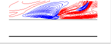
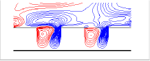
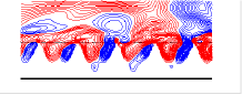
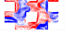
a)                               b)                               c)                               d)
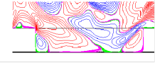
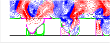
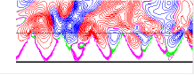
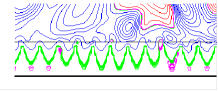
e)                               f)                               g)                               h)

Figure 5: contour plots of $u_{2}$: a) $SM$, b) $TS$, c) $TT$ in planes $x_{1}-x_{2}$, d) $CS$ plane $x_{1}-x_{3}$ at $x_{2}=-1.03$, e) $LLS$, f) $LS$ , g) $LT$, h) $LTS$, planes $x_{3}-x_{2}$, blue and green negative, red and magenta positive $\Delta=0.005$ for red and blue $\Delta=0.0005$ for green and magenta.

The validation of the immersed boundary technique was presented in Orlandi et al. (2006) by a comparison of the pressure distribution on the rod-shaped elements with the measurements by Furuya et al. (1976). These authors studied the boundary layer over circular rods, fixed to the wall transversely to the flow, for several values of $w/k$ ($w$ is the streamwise separation between two consecutive rods of height $k$). The numerical validation was performed for values of $w/k=3,7$ and $15$. It is important to point out that circular rods are appropriate for numerical validation of the immersed boundary method, owing to the variation of the metric along the circle. The numerical simulations were performed, at $Re=U_{P}h/\nu=4200$, and the pressure distributions around the circular rod were compared with those measured. The good agreement reported in Orlandi et al. (2006) implies that the numerical method is accurate and can be used to reproduce the flow past any type of surface. From the physical point of view, the agreement between low $Re$ simulations and high $Re$ experiments ( Furuya et al. (1976)) implies a similarity between the near-wall region of boundary layers and channel flows. In addition it can be asserted that, as in fully rough flows, (Nikuradse (1950)) a Reynolds number independence for the friction factor does exist. The capability of the immersed boundary technique to treat rough surfaces was further demonstrated by a comparison with the experimental results of Burattini et al. (2008) for a flow past transverse square bars with $w/k=3$.

2.2.2 Global results

Several corrugations have been located below the plane of the crest at $x_{2}\pm 1$, that coincides with the walls of channels with smooth walls ($SM$). The shape of the corrugation are given in figure 5 by plotting the contours of the $u_{2}$ velocity component in the planes more appropriate to see the walls of the corrugations. These images demonstrate that the immersed boundary technique accurately reproduces the flow around the corrugations. The velocity component $u_{2}$ coincides with the fluctuating component being, for each realisation, the average in the homogeneous directions equal to zero. In several previous papers it was stressed the importance of the $u_{2}$ fluctuations and the relative statistics. The relevant papers are reported in Orlandi (2013). For the smooth channel the $u_{2}$ contours, in a small region, in figure 5a depict the sweep and the ejection events one after the other. These are the events contributing to increase the drag of turbulent flows with respect to that of laminar flows and to produce turbulent kinetic energy. The recirculating motion in figure 5b within the cavities of the transverse square bars configuration ($TS$), for this spanwise section, connect the negative regions of $u_{2}$ inside with those of the same sign above. However, in a different spanwise section, it has been observed a connection between positive values. The global results leads to a relative high value of $\langle u_{2}^{2}\rangle_{W}$ at the plane of the crests. Triangular transverse bars, one attached to the other ($TT$), generate a more intense recirculating motion (figure 5c)), producing large effects on the overlying turbulent flows. A spanwise coherence of the recirculating motion inside the corrugations is observed, that disappears at a distance $y=0.2$ from the plane of the crests. The capability of the numerical method to describe the complex flow inside the three-dimensional staggered cubes ($CS$) can be appreciated by the contours of $u_{2}$ in figure 5d in a $x_{1}-x_{3}$ plane at $x_{2}=-1.03$ The velocity disturbances ejected from three-dimensional corrugations are large, and, therefore, large effects on the overlying turbulent flow are produced. The motion inside the longitudinal corrugation can be visualised by $u_{2}$ contours in $x_{3}-x_{2}$ planes; in these circumstances the motion is rather weak, therefore contours with $\Delta=0.0005$ are depicted in figures 5e-h in green for negative and in magenta for positive $u_{2}$. These images confirm that the immersed boundary technique reproduces the complexity of the secondary motion, namely for the corrugation $LLS$ (figure 5e) with $w/k=3$ ($w$ is the distance between two square bars), and $LS$ with $w/k=1$. Triangular bars ($LT$) with $s/k=1$ ($s$ is the width of the base of the triangle) in figure 5g show disturbances similar to those in figure 5f for $LS$. On the other hand for the triangular bars with $s/k=0.5$ ($LTS$) the recirculating motion in figure 5h is very weak, and, as a consequence, the activity of the overlying flow decreases, leading to a reduction of turbulent kinetic energy and of the drag.

Flow	$l$	$N_{1}$	$N_{3}$	$H_{fl}$	$R_{\tau}$	$10U_{W}$	$10^{3}<u_{2}^{2}>_{W}$	$10^{2}u_{\tau}$	$10^{3}\tau_{W}$	$10^{3}<u_{1}u_{2}>_{W}$
SM	0	800	128	2.00	204.2	0.0	0.0	4.1678	17.362	0.
CS	1	800	512	2.295	372.1	1.397	3.311	7.5939	15.279	34.985
TT	2	800	128	2.195	313.3	1.048	1.399	6.3942	20.384	16.882
TS	3	800	128	2.190	238.4	0.370	0.157	4.8649	20.000	1.615
LS	4	256	512	2.200	228.8	1.361	0.528	4.6699	13.580	6.245
LLS	5	256	512	2.323	217.2	3.817	0.638	4.4325	4.706	12.206
LT	6	256	512	2.195	205.7	2.691	0.338	4.1981	9.777	6.280
LTS	7	256	512	2.189	166.8	2.143	0.048	3.4040	9.332	1.253

Table 1: Values of some of the global quantities for the simulations at $Re=4900$, the non-uniform grid $x_{2}$ is the same in all cases with $N2=257$ points.

Some of the global results and the resolution for the cases depicted in in figure 5 are reported in the table 1. The resolution in the streamwise and spanwise directions are different for transverse, longitudinal and three-dimensional corrugations. The resolution in $x_{1}$ for transverse corrugations is dictated in order to have $20$ grid points to describe the square and triangular cavities. For the longitudinal corrugations $16$ grid points are used for the solid bars for the $LS$ and $LLS$ cases. For all cases $20$ grid points in the direction $x_{2}$ have been used to get the flow-fields depicted in figure 5. The values of $U_{W}$ (the mean streamwise velocity at the plane of the crests) in the table shows that, $U_{W}$ for the longitudinal bars are greater than those for the transverse corrugations, implying a decrease of $\tau_{W}=\nu{{\partial U}\over{\partial x_{2}}}|_{W}$. Therefore it should be expected a large drag reduction due to this slip condition. As it has been demonstrated by Arenas et al. (2018), if at the plane of the crests the $u_{2}$ can be, ideally, set equal to zero for any kind of corrugations a strong drag reduction is achieved. For the surfaces here considered the largest reduction should be for the $LLS$ configuration. However, in the real flow, the $u_{2}$ fluctuations are large as it can be inferred by the values of $\langle u_{2}^{2}\rangle_{W}$ in table 1. The $u_{2}$ at the plane of the crests generates a turbulent stress $\langle u_{2}u_{1}\rangle_{W}$ which can be considered as a ”form” drag due to the corrugation of the surfaces, contributing to the total resistance $\tau_{T}=\tau_{W}+\langle u_{2}u_{1}\rangle_{W}$. The friction velocities $u_{\tau l}=\sqrt{\tau_{Tl}R_{Vl}}$ ($l$ is an index of the geometry of the surface) show that only for the surface $LTS$ there is a drag reduction with respect to that in presence of smooth walls ($SM$). In this expression $R_{Vl}$ is given by the ratio of $H_{fl}$ with respect to that of the channel with smooth walls ($H$). $H_{fl}$ is the ratio between the volume occupied by the fluid and the area in the homogeneous directions ($L_{1}L_{3}$).

2.2.3 Viscous and turbulent stresses

From the global results it follows that the statistics of large interest are the viscous $\tau=\nu{{\partial U}\over{\partial x_{2}}}$ in figure 6a and the turbulent $-\langle u_{2}u_{1}\rangle$ in figure 6b stresses. The figures are in semi-log form to emphasise the different behavior in the region near the plane of the crests and therefore to enlight the difference with the well known profiles in presence of smooth walls. Figure 6a shows a viscous stress, at the plane of the crests, for transverse grooves higher than that of smooth walls. This occurs despite the presence of a $\widehat{u_{1}}|_{W}\neq 0$ in the regions of the cavities. The over-script $\widehat{\cdot}$ indicates an average in time, in $x_{3}$ for the transverse, in $x_{1}$ for the longitudinal corrugations of the generic quantity $q(x_{1},x_{2},x_{3},t)$. A further phase average over several elements allows to have the distribution of $\widehat{u_{1}}|_{W}$ along the cavity. The distribution of $\widehat{u_{1}}|_{W}$ and of $\widehat{u_{1}}$ above the cavities varies with the type of corrugations and thus allow to understand which part of the cavity contributes more to the reduction of ${{\partial\widehat{u_{1}}}\over{\partial y}}|_{W}$. Orlandi et al. (2016), for the $TS$ and $TT$ surfaces, described in detail the reduction of the viscous stress above the cavity region and the large increase near the solid leading to the values of $\tau$ in figure 6a higher than that of $SM$. Similar distribution along each transverse cavity for $\widehat{u_{1}u_{2}}|_{W}$ demonstrate why, in figure 6b, a small for $TS$, and a large for $TT$, values are found. The latter is due to the strong ejections flowing along the slopes of the triangular cavities (figure 5c). For $TT$ the profiles of the viscous and the turbulent stress largely differ from those in presence of smooth walls. The statistics profiles are those typical of $k$ type roughness. Instead for the $TS$ surface the profiles are those typical of ”d” type roughness. The turbulent stress profile for the flow past staggered cubes ($CS$) is the largest among all the cases here studied with a maximum four times greater than that of smooth walls. Even in this flow the causes of the increase are due to the flow ejections from the roughness layer, qualitatively depicted in figure 5d. The viscous stress profiles of the longitudinal corrugations in figure 6a are largely reduced with respect to that of the smooth wall, with the smallest values for $LLS$ due to the high $\widehat{u_{1}}|_{W}$ generated at the wide interface of the cavity. Figure 5e shows a rather high $u_{2}$ inside the cavity leading to a turbulent stress three times greater than the viscous stress at the plane of the crests. The final result leads to a friction velocity slightly higher than that of smooth walls. The other two surfaces $LT$ and $LS$, despite the different profiles of the two stresses, lead to similar values of $u_{\tau}$ in table 1. The recirculating motion inside the $LS$ cavity (figure 5f) is similar to that inside the $LT$ (figure 5g), therefore the turbulent stress at the plane of the crest in figure 6b is the same. The wider solid surface of $LS$ is the reason why $u_{\tau}$ in table 1 is slightly greater than that for $LT$. Thin triangular cavities, as those in figure 5h ($LTS$), give at the plane of the crests the same value of the viscous stress of $LT$, on the other hand the values of turbulent stress, in figure 6b, are drastically reduced in the whole channel leading to a sensible drag reduction. In fact for $LTS$ $u_{\tau}$ is $18\%$ smaller than for $SM$.

\psfrag{ylab}{ \large$\tau$}\psfrag{xlab}{ $y$}\includegraphics[width=213.39566pt]{fig6_a.eps}

\psfrag{ylab}{ \large$\tau$}\psfrag{xlab}{ $y$}\psfrag{ylab}{ \large$-\langle u_{2}u_{1}\rangle$}\psfrag{xlab}{ $y$}\includegraphics[width=213.39566pt]{fig6_b.eps}

a)                                                             b) \psfrag{ylab}{ \large$\tau$}\psfrag{xlab}{ $y$}\psfrag{ylab}{ \large$-\langle u_{2}u_{1}\rangle$}\psfrag{xlab}{ $y$}\psfrag{ylab}{ \large$\langle u_{2}^{2}\rangle^{+}$}\psfrag{xlab}{ $y^{+}$}\includegraphics[width=213.39566pt]{fig6_c.eps} \psfrag{ylab}{ \large$\tau$}\psfrag{xlab}{ $y$}\psfrag{ylab}{ \large$-\langle u_{2}u_{1}\rangle$}\psfrag{xlab}{ $y$}\psfrag{ylab}{ \large$\langle u_{2}^{2}\rangle^{+}$}\psfrag{xlab}{ $y^{+}$}\psfrag{ylab}{ \large$U^{+}-U_{W}^{+}$}\psfrag{xlab}{ $y^{+}$}\includegraphics[width=213.39566pt]{fig6_d.eps}                                            c)                                                             d)

Figure 6: Profiles of: a) viscous stress, b) turbulent stress versus the distance from the plane of the crests, in computational units; c) the normal to the wall stress, d) the mean velocity subtracted to the velocity at the plane of the crests $U_{W}$, in c) and d) the statistics and the distance are in wall units. The flows listed in the insets of a) corresponds to those in table 1.

Our view is that the normal to the wall stress is the fundamental statistics to characterise wall bounded flows. The values at the plane of the crests are linked to the shape of the surfaces. It should be a difficult task to relate it to the kind of the surface, in fact a large number of geometrical parameters enter in the characterisation of a surface. For instance in figure 6c the profile of $\langle u_{2}^{2}\rangle$ of $LTS$ do not differ from that of $TS$ being the surfaces completely different. Despite the quantitative differences with the smooth wall it is interesting to notice that, in a thin layer of few wall units, the growth is similar to that for smooth walls, with the exception of the surfaces with very strong ejections ($CS$ and $TT$). Orlandi (2013) by investigating the importance of $\langle u_{2}^{2}\rangle|_{W}$ in wall bounded flows observed that the roughness function $\Delta U^{+}$ evaluated by the profiles of $U^{+}-U_{W}^{+}$ is proportional to $\langle u_{2}^{2}\rangle^{+}|_{W}$. This behavior can be appreciated in figure 6d where the downward shift of the $\log$ law is greater higher $\langle u_{2}^{2}\rangle^{+}|_{W}$. In figure 6d the results by Lee & Moser (2015) are in perfect agreement with the present one corroborating the accuracy of the present numerics. The differences, in figure 6c, between the present $SM$ and the Lee & Moser (2015) profiles should be, in part, attributed to the effect of the Reynolds number. In fact, in the previous section, large differences have been observed at low $Re$, here $R_{\tau}=204$ instead in Lee & Moser (2015) $R_{\tau}=180$.

\psfrag{ylab}{\large$q^{2+}$}\psfrag{xlab}{\large$$ }\includegraphics[width=213.39566pt]{fig7_a.eps}

\psfrag{ylab}{\large$q^{2+}$}\psfrag{xlab}{\large$$ }\psfrag{ylab}{\large$\epsilon^{+}$ }\psfrag{xlab}{\large$$ }\includegraphics[width=213.39566pt]{fig7_b.eps}

a)                                                             b) \psfrag{ylab}{\large$q^{2+}$}\psfrag{xlab}{\large$$ }\psfrag{ylab}{\large$\epsilon^{+}$ }\psfrag{xlab}{\large$$ }\psfrag{ylab}{\large$(q^{2}/\epsilon)^{+}$}\psfrag{xlab}{\large$y^{+}$ }\includegraphics[width=213.39566pt]{fig7_c.eps} \psfrag{ylab}{\large$q^{2+}$}\psfrag{xlab}{\large$$ }\psfrag{ylab}{\large$\epsilon^{+}$ }\psfrag{xlab}{\large$$ }\psfrag{ylab}{\large$(q^{2}/\epsilon)^{+}$}\psfrag{xlab}{\large$y^{+}$ }\psfrag{ylab}{\large$Sq^{2}/\epsilon$}\psfrag{xlab}{\large$y^{+}$ }\includegraphics[width=213.39566pt]{fig7_d.eps}                                            c)                                                             d)

Figure 7: Profiles in wall units of: a) turbulent kinetic energy, b) rate of isotropic dissipation, c) eddy turnover time, d) shear parameter for the flows with rough surfaces listed in the inset in a), compared with those in presence of smooth walls (open circle present at $R_{\tau}=204$, lines Lee & Moser (2015) at $R_{\tau}=180$).

2.2.4 Shear parameter

For flows past smooth walls despite the $Re$ variations in the near-wall region of the turbulent kinetic energy and of the rate of energy dissipation in figure 1c there was a good scaling of the eddy turnover time. Figure 7a shows unexpected behavior of $q^{2+}$ depending on the type of roughness. For instance it is rather difficult to predict the large increase of $q^{2+}$ for $LLS$ with respect to that for $CS$ being the differences between the $\langle u_{2}u_{2}\rangle^{+}$ in figure 6c rather small. The profiles of each normal stress, not reported, show that the growth of $q^{2+}$ is due to the large increase of $\langle u_{1}u_{1}\rangle^{+}$. The increase of $\langle u_{3}u_{3}\rangle^{+}$, instead, is moderate. The message of figure 7a is that in the near-wall region the longitudinal grooves generate values of $q^{2+}$ greater than those for transverse and three-dimensional corrugations, due to the large streamwise fluctuations inside the longitudinal cavities. In figure 7b large variations in the near-wall region of the profiles of the rate of dissipation do not have the same trend as those of $q^{2+}$. The $LS$ and the $TS$ surfaces have a high rate of dissipation, in the near-wall region, due to large amount of solid at the plane of the crests, generating high $s_{12}^{2+}$ contributing more to $\epsilon^{+}$ than the other fluctuating shears. Only for the $LTS$ flow the small fluctuations near the plane of the crests, and the small amount of solid give rise to a rate of dissipation smaller than that of the smooth wall. The profile of the eddy turnover time of the $TS$ surface, in figure 7c, is the only one close to that of smooth walls and the difference is mainly due to the $\epsilon^{+}$ in figure 7b. Interestingly figure 7c depicts a completely different behavior for transverse and longitudinal corrugations. In the latter $q^{2+}/\epsilon^{+}$ remains constant while in the former it decays similarly to the smooth walls. The shear parameter $S^{*}$ corroborates the similarity between the smooth and the $TS$ surface, classified as ”d” type roughness, with a weak drag increase with respect to $SM$. In both surfaces as well as for $LTS$ with drag reduction the maximum is located approximately at $y^{+}=10$. Flow visualizations for $LTS$ depicts the formation of streaky structures similar to those of the smooth channel. For the other longitudinal corrugations the maximum of $S^{*}$, near the plane of the crests, depend on the type of surface, indicating that the shape of the surface dictates the structures formation. The values of $S^{*}$ suggest that for $LS$ the longitudinal structures are coherent, these become more strong and coherent for the $LLS$ surfaces. The low values $S^{*}$ indicate an isotropization of the structures, that was investigated by Orlandi & Leonardi (2006) through the profiles of the normal stresses. In figure 7e the collapse of the $S^{*}$ profiles in the outer layer, despite the differences near the plane of the crests, is a first indication of the validity of the Townsend similarity hypothesis (Townsend (1976)).

\psfrag{ylab}{\hskip-28.45274pt\large$(10^{2}{{d^{2}\langle{u_{2}^{2}}\rangle}\over{dx^{2}_{2}}})^{+}$}\psfrag{xlab}{ $y^{+}$}\includegraphics[width=213.39566pt]{fig8_a.eps}

\psfrag{ylab}{\hskip-28.45274pt\large$(10^{2}{{d^{2}\langle{u_{2}^{2}}\rangle}\over{dx^{2}_{2}}})^{+}$}\psfrag{xlab}{ $y^{+}$}\psfrag{ylab}{\large$\langle\omega_{2}^{2}\rangle^{+}$}\psfrag{xlab}{\large$y^{+}$ }\includegraphics[width=213.39566pt]{fig8_b.eps}

a)                                                             b)

Figure 8: Profiles in wall units of: a) ${{d^{2}\langle{u_{2}^{2}}\rangle}\over{dx^{2}_{2}}}$, b) $rms$ of normal to the wall vorticity component, for the flows with rough surfaces listed in the inset of a), compared with those in presence of smooth walls (open circle present at $R_{\tau}=204$, lines Lee & Moser (2015) at $R_{\tau}=180$).

2.2.5 Structural statistics

As for the smooth channel the analysis of the kind of structures near the surfaces can be drawn by the profiles of $({{d^{2}\langle{u_{2}^{2}}\rangle}\over{dx^{2}_{2}}})^{+}$. It is worth to recall that positive values indicate a layer dominated by sheet-like and negative by rod-like structures. In figure 8 as well as in figure 7b differences can be noticed between the present $SM$ data and those at $R_{\tau}=180$ in figure 2a. The reason should be ascribed in a large measure to the different $R_{\tau}$ and in a reduced measure to the coarse grid, here used to have a smooth transition of the resolution in the flow side with that required to reproduce the roughness layer. The resolution and the Reynolds number affect more the profiles of $\langle\omega_{2}^{2}\rangle^{+}$ in figure 8b and of $\epsilon^{+}$ in figure 7b. Both figures 8 show drastic differences between smooth and rough walls in the inner region that disappear in the outer region. For the longitudinal corrugations, near the plane of the crests, and, in particular, in contact with the solid tubular-like structures form, as it is qualitatively depicted by the $u_{2}$ contours in figure 5. Even for the transverse triangular bar ($TT$) as well as for the cubes ($CS$) there is a tendency to the formation of tubular-like structures. For flow past the $TS$ surface, on the other hand, there is a prevalence of the sheet-like structures even higher than that for smooth walls ($SM$). This can be also deduced by comparing figure 5c and figure 5d. Only the $LLS$ flow shows small variations of $-{\langle Q\rangle}$, and once more this occurrence is corroborated by the smooth contours in figure 5e of $u_{2}$ lying in large structures. The intensification of the contours of $u_{2}$ near the wedges in figure 5f and figure 5g, relative to the longitudinal corrugations $LLS$ and $LT$, explain the negative values of $-{\langle Q\rangle}$ near the plane of the crests in figure 8a. The locations where $-{\langle Q\rangle}=0$ vary between $y^{+}=10$ and $y^{+}=18$, in correspondence of this region the maximum of turbulent kinetic energy production is located, as discussed later on.

Near smooth walls the elongated structures, the so called near-wall streaks usually are characterised by regions of negative and positive $u_{1}$. The same picture is obtained by contours of $\omega_{2}$, therefore it is interesting to look at the effects of the shape of the surfaces on the profiles of $\langle\omega_{2}^{2}\rangle^{+}$. In presence of smooth walls the streaky structures are very intense at the distance where these are generated, accordingly the peak of $\langle\omega_{2}^{2}\rangle^{+}$ is located at $y^{+}\approx 15$. Figure 8b shows a different trend, near the plane of the crests, between the longitudinal and the transverse corrugations. For the $TT$ and the $CS$ surfaces the small and constants values of $\langle\omega_{2}^{2}\rangle^{+}$ suggest an isotropization of the small scales in the near wall region. In the near-wall region the isotropization is further corroborated by the profiles of the three vorticity $rms$, not shown. These profiles do not depict the large differences among the three components reported by Kim et al. (1987) for the channel with smooth walls. On the other hand, for the longitudinal grooves the anisotropy of the structures is appreciated by the growth of $\langle\omega_{2}^{2}\rangle^{+}$ moving towards the plane of the crests. The strong planar motion at the top of the cavities, in particular for the $LS$ and $LT$ surfaces causes this growth. This motion is due to the the large $u_{2}$ fluctuations generated inside the longitudinal cavities depicted in figure 5f and figure 5g. For the drag reducing surface ($LTS$) these fluctuations reduce in the near-wall region (figure 5h), therefore the strength of small and large scales reduce in accord to the decrease of $q^{2+}$ and $\epsilon^{+}$ in figure 7. In figure 8b $\langle\omega_{2}^{2}\rangle^{+}$ for $LTS$ is smaller than that of the other longitudinal corrugations.

2.2.6 Flow visualizations and statistics

The surface contours of $\omega_{2}$, in the near-wall region, for the different corrugations may be of help to explain what has been previously discussed . The visualizations are performed by taking only one realisation, from which the $rms$ profiles of $\langle\omega_{2}^{2}\rangle$ are calculated. The comparison between these profiles, indicated by lines, and those calculated by taking several fields, indicated by symbols, demonstrates that the main features, previously described by converged statistics, are captured by one realisation. This is shown in figure 9a and in figure 9b through the profiles of $\langle u_{2}^{2}\rangle$ and of $\langle\omega_{2}^{2}\rangle$ in computational units. These profiles show, in figure 9a, that, $\langle u_{2}^{2}\rangle$ is rather constant near the plane of the crests, and $\langle\omega_{2}^{2}\rangle$ depends on the type of corrugations. In some of the flows, and, in particular, for those with a large resistance or those with large longitudinal corrugations ($LLS$) $\langle\omega_{2}^{2}\rangle$ decreases moving far from the plane of the crests. For transverse corrugations $\langle\omega_{2}^{2}\rangle$ increases as for smooth walls. It remains constant in a thick layer for the drag reducing flow ($LTS$). The weak $u_{2}$ fluctuations created by the $TS$ corrugation do not produce large differences in the near-wall streaks, as it can be appreciated by comparing figure 9c for $SM$ and figure 9d for $TS$. On the other hand, the strong $u_{2}$ fluctuations emerging from the $CS$ and the $TT$ surfaces break the streamwise coherence of the near wall structures emphasised in figure 9e ($TT$) and in figure 9f ($CS$).

\psfrag{ylab}{\hskip-28.45274pt\large$\langle{u_{2}^{2}}\rangle$}\psfrag{xlab}{ $y$}\includegraphics[width=213.39566pt]{fig9_a.eps}

\psfrag{ylab}{\hskip-28.45274pt\large$\langle{u_{2}^{2}}\rangle$}\psfrag{xlab}{ $y$}\psfrag{ylab}{\large$\langle\omega_{2}^{2}\rangle$}\psfrag{xlab}{\large$y$ }\includegraphics[width=213.39566pt]{fig9_b.eps}

a)                                                             b) \psfrag{ylab}{\hskip-28.45274pt\large$\langle{u_{2}^{2}}\rangle$}\psfrag{xlab}{ $y$}\psfrag{ylab}{\large$\langle\omega_{2}^{2}\rangle$}\psfrag{xlab}{\large$y$ }\includegraphics[width=113.81102pt]{o2fl_smoo.eps} \psfrag{ylab}{\hskip-28.45274pt\large$\langle{u_{2}^{2}}\rangle$}\psfrag{xlab}{ $y$}\psfrag{ylab}{\large$\langle\omega_{2}^{2}\rangle$}\psfrag{xlab}{\large$y$ }\includegraphics[width=113.81102pt]{o2fl_sqt.eps} \psfrag{ylab}{\hskip-28.45274pt\large$\langle{u_{2}^{2}}\rangle$}\psfrag{xlab}{ $y$}\psfrag{ylab}{\large$\langle\omega_{2}^{2}\rangle$}\psfrag{xlab}{\large$y$ }\includegraphics[width=113.81102pt]{o2fl_trt.eps} \psfrag{ylab}{\hskip-28.45274pt\large$\langle{u_{2}^{2}}\rangle$}\psfrag{xlab}{ $y$}\psfrag{ylab}{\large$\langle\omega_{2}^{2}\rangle$}\psfrag{xlab}{\large$y$ }\includegraphics[width=113.81102pt]{o2fl_prsh.eps} c)                           d)                           e)                           f) \psfrag{ylab}{\hskip-28.45274pt\large$\langle{u_{2}^{2}}\rangle$}\psfrag{xlab}{ $y$}\psfrag{ylab}{\large$\langle\omega_{2}^{2}\rangle$}\psfrag{xlab}{\large$y$ }\includegraphics[width=113.81102pt]{o2fl_sqll.eps} \psfrag{ylab}{\hskip-28.45274pt\large$\langle{u_{2}^{2}}\rangle$}\psfrag{xlab}{ $y$}\psfrag{ylab}{\large$\langle\omega_{2}^{2}\rangle$}\psfrag{xlab}{\large$y$ }\includegraphics[width=113.81102pt]{o2fl_sql.eps} \psfrag{ylab}{\hskip-28.45274pt\large$\langle{u_{2}^{2}}\rangle$}\psfrag{xlab}{ $y$}\psfrag{ylab}{\large$\langle\omega_{2}^{2}\rangle$}\psfrag{xlab}{\large$y$ }\includegraphics[width=113.81102pt]{o2fl_trl.eps} \psfrag{ylab}{\hskip-28.45274pt\large$\langle{u_{2}^{2}}\rangle$}\psfrag{xlab}{ $y$}\psfrag{ylab}{\large$\langle\omega_{2}^{2}\rangle$}\psfrag{xlab}{\large$y$ }\includegraphics[width=113.81102pt]{o2fl_trls.eps} g)                           h)                           i)                           l)

Figure 9: Profiles in computational units of the $rms$ of the: a) normal to the wall velocity, b) normal to the wall vorticity components, for the flows with rough surfaces listed in the inset of b), symbols averages in time and in the homogeneous directions $x_{1}$ and $x_{3}$, lines the same quantities averaged in $x_{1}$ and $x_{3}$ of the fields used to get the visualizations of $\omega_{2}$ (red $\omega_{2}=+1$, yellow $\omega_{2}=-1$): c) $SM$, d) $TS$, e) $TT$, f) $CS$ , g) $LLS$, h) $LS$, i) $LT$, l) $LTS$

The $\omega_{2}$ contours are clustered in short regions. The tendency towards the isotropization of the small scales is also corroborated by visualizations, not shown of $\omega_{1}$ and $\omega_{3}$. The impact of the geometry surfaces on the $\omega_{2}$ vorticity is depicted in figure 9g by the positive and negative surface contours of $\omega_{2}$ attached to the corners of $LLS$, spanning the entire length in the streamwise direction. These vorticity layers are generated by the strong $\frac{\partial u_{1}}{\partial x_{3}}$ forming near the vertical walls inside the cavities. A similar view is obtained in the $LS$ (figure 9h) and $LT$ (figure 9i) flows by the layers of $\omega_{2}$ generated near the cavities walls. For $LT$ the $\omega_{2}$ layers are less intense than those for $LS$, accordingly to the profiles in figure 9b. In the drag reducing $LTS$ flow the weak motion near the plane of the crest creates a more uniform flow and therefore the vorticity structures in figure 9l are weak.

2.2.7 Turbulent kinetic energy production

\psfrag{ylab}{ \large$R_{\alpha\alpha}^{+}$}\psfrag{xlab}{ $$}\includegraphics[width=213.39566pt]{fig10_a.eps}

\psfrag{ylab}{ \large$R_{\alpha\alpha}^{+}$}\psfrag{xlab}{ $$}\psfrag{ylab}{\large$R_{\gamma\gamma}^{+}$}\psfrag{xlab}{ $$}\includegraphics[width=213.39566pt]{fig10_b.eps}

a)                                                             b) \psfrag{ylab}{ \large$R_{\alpha\alpha}^{+}$}\psfrag{xlab}{ $$}\psfrag{ylab}{\large$R_{\gamma\gamma}^{+}$}\psfrag{xlab}{ $$}\psfrag{ylab}{\large$P_{\alpha}^{+}$}\psfrag{xlab}{\large$$ }\includegraphics[width=213.39566pt]{fig10_c.eps} \psfrag{ylab}{ \large$R_{\alpha\alpha}^{+}$}\psfrag{xlab}{ $$}\psfrag{ylab}{\large$R_{\gamma\gamma}^{+}$}\psfrag{xlab}{ $$}\psfrag{ylab}{\large$P_{\alpha}^{+}$}\psfrag{xlab}{\large$$ }\psfrag{ylab}{\large$P_{\gamma}^{+}$}\psfrag{xlab}{\large$$ }\includegraphics[width=213.39566pt]{fig10_d.eps}                                            c)                                                             d) \psfrag{ylab}{ \large$R_{\alpha\alpha}^{+}$}\psfrag{xlab}{ $$}\psfrag{ylab}{\large$R_{\gamma\gamma}^{+}$}\psfrag{xlab}{ $$}\psfrag{ylab}{\large$P_{\alpha}^{+}$}\psfrag{xlab}{\large$$ }\psfrag{ylab}{\large$P_{\gamma}^{+}$}\psfrag{xlab}{\large$$ }\psfrag{ylab}{\large$P_{k}^{+}$}\psfrag{xlab}{\large$y^{+}$ }\includegraphics[width=213.39566pt]{fig10_e.eps} \psfrag{ylab}{ \large$R_{\alpha\alpha}^{+}$}\psfrag{xlab}{ $$}\psfrag{ylab}{\large$R_{\gamma\gamma}^{+}$}\psfrag{xlab}{ $$}\psfrag{ylab}{\large$P_{\alpha}^{+}$}\psfrag{xlab}{\large$$ }\psfrag{ylab}{\large$P_{\gamma}^{+}$}\psfrag{xlab}{\large$$ }\psfrag{ylab}{\large$P_{k}^{+}$}\psfrag{xlab}{\large$y^{+}$ }\psfrag{ylab}{\large$D_{k}^{+}$}\psfrag{xlab}{\large$y^{+}$ }\includegraphics[width=213.39566pt]{fig10_f.eps}                                            e)                                                             f)

Figure 10: Profiles in wall units of the stress aligned with: a) $S_{\alpha}$, b) $S_{\gamma}$, of the turbulent kinetic energy production aligned with c) $S_{\alpha}$, d) $S_{\gamma}$, e) turbulent kinetic energy production, f) full rate of dissipation $D_{k}^{+}$, for the flows with rough surfaces listed in the inset of a), compared with those in presence of smooth walls (open circle present at $R_{\tau}=204$, lines Lee & Moser (2015) at $R_{\tau}=180$).

The large dependence of the statistics upon the shape of the corrugations should be also observed in the components of the normal stresses aligned with the eigenvectors of the strain tensor $S_{ij}$. As for smooth walls, in this reference system the stress $R_{\gamma\gamma}$ aligned with the compressive $S_{\gamma}$ and the $R_{\alpha\alpha}$ aligned with the extensional $S_{\alpha}$ strain become of the same order. The stress in the spanwise direction ($R_{33}$), does not change, and coincide with $R_{\beta\beta}$ aligned with $S_{\beta}=0$. For any surface figure 10a and figure 10b show that the stress aligned with $S_{\gamma}$ are greater than those aligned with $S_{\alpha}$. For the longitudinal corrugations $R_{\alpha\alpha}$ and $R_{\gamma\gamma}$ become very large. This is mainly due to the growth of $R_{11}$ in particular for the $LLS$ surface. In this reference system no one component has a constant trend near the plane of the crests as that in figure 9a. The $R_{\alpha\alpha}$ and the $R_{\gamma\gamma}$ grow or decrease with slopes that depend on the shape of the surface. The slope is zero for the $LT$ surface. This stress decomposition allows to split the turbulent kinetic production $P_{k}=-(P_{\gamma}+P\alpha)$; in magnitude $P_{\gamma}$ in figure 10d, is greater than $P\alpha$, in figure 10c. Near the walls the two component have a similar trend with the highest values for the $LLS$ due to the strong fluctuations generated within the cavities. The increase of $R_{\alpha\alpha}$ and $R_{\gamma\gamma}$ despite the reduction of $S_{\alpha}$ and $S_{\gamma}$ leads to the increase of $P^{+}_{\alpha}$ and of $P_{\gamma}^{+}$. For the drag reducing surface the components of $P_{k}$ decrease. These are rather small for the three dimensional corrugations. The same trend should be expected for $P_{k}$, on the other hand, figure 10e shows a different trend with maximum production for $TT$ and a sensible reduction for $LLS$ and $LS$ corrugations. In some of the flows the maximum production is located near the plane of the crests, with the exception of the $LTS$ and $TS$ surfaces, which do not differ much with the $P_{k}$ profile in presence of smooth walls. The rate of isotropic dissipation $\epsilon^{+}$ in the near wall region, in figure 7b, is greater than the production $P_{k}^{+}$. The trend of the maximum of $\epsilon^{+}$ are not similar to those of the production $P_{k}^{+}$. Near smooth walls, in figure 2, the same trend for the profiles of $P_{k}^{+}$ and $D_{k}^{+}$ was observed and the difference between the two was balanced by the turbulent diffusion $T_{k}^{+}$ due to the non-linear terms. In figure 10f $D_{k}^{+}$ has been plotted showing a complex behavior. For the $CS$, $LT$, $LTS$ and $LS$ corrugations a trend similar to that of $P_{k}^{+}$ is found while for the other flows large differences occurs. Therefore very large differences should be expected in the profiles of $T_{k}^{+}$.

\psfrag{ylab}{ \hskip-14.22636pt$BUDG^{+}$}\psfrag{xlab}{\large$$ }\includegraphics[width=213.39566pt]{fig11_a.eps}

\psfrag{ylab}{ \hskip-14.22636pt$BUDG^{+}$}\psfrag{xlab}{\large$$ }\psfrag{ylab}{\large$$}\psfrag{xlab}{\large$$ }\includegraphics[width=213.39566pt]{fig11_b.eps}

a)                                                             b) \psfrag{ylab}{ \hskip-14.22636pt$BUDG^{+}$}\psfrag{xlab}{\large$$ }\psfrag{ylab}{\large$$}\psfrag{xlab}{\large$$ }\psfrag{ylab}{\large$$}\psfrag{xlab}{\large$$ }\includegraphics[width=213.39566pt]{fig11_c.eps} \psfrag{ylab}{ \hskip-14.22636pt$BUDG^{+}$}\psfrag{xlab}{\large$$ }\psfrag{ylab}{\large$$}\psfrag{xlab}{\large$$ }\psfrag{ylab}{\large$$}\psfrag{xlab}{\large$$ }\psfrag{ylab}{\large$$}\psfrag{xlab}{\large$$ }\includegraphics[width=213.39566pt]{fig11_d.eps}                                            c)                                                             d) \psfrag{ylab}{ \hskip-14.22636pt$BUDG^{+}$}\psfrag{xlab}{\large$$ }\psfrag{ylab}{\large$$}\psfrag{xlab}{\large$$ }\psfrag{ylab}{\large$$}\psfrag{xlab}{\large$$ }\psfrag{ylab}{\large$$}\psfrag{xlab}{\large$$ }\psfrag{ylab}{ \hskip-14.22636pt$BUDG^{+}$}\psfrag{xlab}{\large$y^{+}$ }\includegraphics[width=213.39566pt]{fig11_e.eps} \psfrag{ylab}{ \hskip-14.22636pt$BUDG^{+}$}\psfrag{xlab}{\large$$ }\psfrag{ylab}{\large$$}\psfrag{xlab}{\large$$ }\psfrag{ylab}{\large$$}\psfrag{xlab}{\large$$ }\psfrag{ylab}{\large$$}\psfrag{xlab}{\large$$ }\psfrag{ylab}{ \hskip-14.22636pt$BUDG^{+}$}\psfrag{xlab}{\large$y^{+}$ }\psfrag{ylab}{\large$$}\psfrag{xlab}{\large$y^{+}$ }\includegraphics[width=213.39566pt]{fig11_f.eps}                                            e)                                                             f) \psfrag{ylab}{ \hskip-14.22636pt$BUDG^{+}$}\psfrag{xlab}{\large$$ }\psfrag{ylab}{\large$$}\psfrag{xlab}{\large$$ }\psfrag{ylab}{\large$$}\psfrag{xlab}{\large$$ }\psfrag{ylab}{\large$$}\psfrag{xlab}{\large$$ }\psfrag{ylab}{ \hskip-14.22636pt$BUDG^{+}$}\psfrag{xlab}{\large$y^{+}$ }\psfrag{ylab}{\large$$}\psfrag{xlab}{\large$y^{+}$ }\psfrag{ylab}{ \hskip-14.22636pt$BUDG^{+}$}\psfrag{xlab}{\large$y^{+}$ }\includegraphics[width=213.39566pt]{fig11_g.eps} \psfrag{ylab}{ \hskip-14.22636pt$BUDG^{+}$}\psfrag{xlab}{\large$$ }\psfrag{ylab}{\large$$}\psfrag{xlab}{\large$$ }\psfrag{ylab}{\large$$}\psfrag{xlab}{\large$$ }\psfrag{ylab}{\large$$}\psfrag{xlab}{\large$$ }\psfrag{ylab}{ \hskip-14.22636pt$BUDG^{+}$}\psfrag{xlab}{\large$y^{+}$ }\psfrag{ylab}{\large$$}\psfrag{xlab}{\large$y^{+}$ }\psfrag{ylab}{ \hskip-14.22636pt$BUDG^{+}$}\psfrag{xlab}{\large$y^{+}$ }\psfrag{ylab}{\large$$}\psfrag{xlab}{\large$y^{+}$ }\includegraphics[width=213.39566pt]{fig11_h.eps}                                            g)                                                             h)

Figure 11: Profiles in wall units of the simplified budgets: $D_{k}=\nu\langle u_{i}\nabla^{2}u_{i}\rangle$ , $P_{k}=-2\langle u_{2}u_{1}\rangle S$, $T_{k}=-({{d\langle u_{2}u_{i}^{2}\rangle}\over{dx_{2}}}+\langle u_{i}\frac{\partial p}{\partial x_{i}}\rangle)$ a) $SM$ , b) $TS$ , c) $TT$, d) $CS$ , e) $LLS$, f) $LS$ , g) $LT$, h) $LTS$; in a) line Lee & Moser (2015) at $R_{\tau}=180$ symbols present $R_{\tau}=204$.

2.2.8 Budgets of turbulent kinetic energy

To emphasise the differences in the turbulent kinetic energy budgets in presence of rough surfaces with respect to that of smooth walls the simplified budget is considered. In these circumstances the production is balanced by $D_{k}$ and by the turbulent diffusion due to the non-linear terms and to the correlations between velocity and pressure gradients. For smooth walls all the terms are equal to zero at the wall and grow with a different trend; $|D_{k}|$ and $T_{k}$ proportionally to $y^{2}$ and $P_{k}$ to $y^{3}$. The $T_{k}$ is positive in the region with $-{\langle Q\rangle}>0$ meaning that the sheet-like structures loose energy towards the region with $-{\langle Q\rangle}<0$ where the tubular-like structures prevail. This is depicted in figure 11a with the present data compared with those of Lee & Moser (2015) at $R_{\tau}=180$. The agreement is rather good, the small differences in $D_{k}^{+}$ and $T_{k}^{+}$ are due to the different Reynolds numbers and to the coarse resolution near the surface in this simulation. The transverse square bars $TS$ show a similar trend in figure 11b with the difference to get the three terms different from zero at the plane of the crests. This occurrence is due to the small velocity fluctuations generated inside the square cavities. In presence of triangular bars ($TT$) the strong fluctuations emerging from the cavities produce a high $\langle u_{1}u_{2}\rangle_{W}$; the maximum production, in figure 11c, moves at the plane of the crests with the consequence to have there a high $D_{k}^{+}$. In this flow the turbulent transfer is low and negative near the plane of the crests. This negative contribution is balanced by the positive contribution at the center of the channel. It is worth to recall that for smooth walls the total contribution of the turbulent transfer is null, for rough surfaces it is smaller than the total production and full rate of dissipation, but it could be different from zero. For the $CS$ surface figure 11d shows a reduction of $P_{k}^{+}$ and $D_{k}^{+}$ near the plane of the crests. The large disturbances emerging from the interior of the surfaces make $T_{K}^{+}$ a sink of energy comparable to the total rate of dissipation. This is corroborated by the large values $-{\langle Q\rangle}<0$ in figure 8a implying the prevalence of tubular-like structures in this layer. For the $LLS$ corrugation the wide cavity generates large $u_{2}$ fluctuations, therefore the turbulent transfer is a sink of turbulent kinetic energy and greater than $D_{k}^{+}$ (figure 11e), implying the formation of tubular-like structures near the plane of the crests, as it was depicted in figure 8a. Figure 9a shows that the $\langle u^{2}_{2}\rangle$ for $LS$ does not change too much with respect to that for $LLS$ and therefore the $T_{k}^{+}$ profile in figure 11f is similar to that in figure 11e. For $LS$ the increase of solid at the plane of the crests leads to an increase of $S$ greater than the reduction of $\langle u_{2}u_{1}\rangle$, as it is shown in figure 6a and figure 6b. This occurrence explain the increase of $P_{k}^{+}$ and $D_{k}^{+}$ in figure 11f with respect to the quantities calculated near the plane of the crests for $LLS$. For the triangular ($LT$) as well as for the square ($LS$) longitudinal bars, $T_{K}^{+}$ is negative in a large part of the channel. In figure 11g the values of $T_{k}^{+}$ are small, therefore the energy produced is directly dissipated. For the $LTS$ the $u_{2}$ fluctuations reduce with respect to those generated in the $LT$ corrugations (figure 9a), in addition the profiles of $-{\langle Q\rangle}$ for $LTS$ in figure 8a are similar to those for $TS$ and consequently the budgets in figure 11h do not differ too much from those in figure 11b.

\psfrag{ylab}{ $\nu_{T}^{+}$}\psfrag{xlab}{ $y^{+}$}\includegraphics[width=213.39566pt]{fig12_a.eps}

\psfrag{ylab}{ $\nu_{T}^{+}$}\psfrag{xlab}{ $y^{+}$}\psfrag{ylab}{\hskip 0.0pt$\nu_{T}|^{+}_{W}$}\psfrag{xlab}{ $v^{\prime+}_{W}$}\includegraphics[width=213.39566pt]{fig12_b.eps}

a)                                                             b) \psfrag{ylab}{ $\nu_{T}^{+}$}\psfrag{xlab}{ $y^{+}$}\psfrag{ylab}{\hskip 0.0pt$\nu_{T}|^{+}_{W}$}\psfrag{xlab}{ $v^{\prime+}_{W}$}\psfrag{ylab}{ $\Delta U^{+}$}\psfrag{xlab}{ $v^{\prime+}_{W}$}\includegraphics[width=213.39566pt]{fig12_c.eps} \psfrag{ylab}{ $\nu_{T}^{+}$}\psfrag{xlab}{ $y^{+}$}\psfrag{ylab}{\hskip 0.0pt$\nu_{T}|^{+}_{W}$}\psfrag{xlab}{ $v^{\prime+}_{W}$}\psfrag{ylab}{ $\Delta U^{+}$}\psfrag{xlab}{ $v^{\prime+}_{W}$}\psfrag{ylab}{ $K_{S}^{+}$}\psfrag{xlab}{ $v^{\prime+}_{W}$}\includegraphics[width=213.39566pt]{fig12_d.eps}                                            c)                                                             d)

Figure 12: Profiles in wall units of: a)$\nu_{T}^{+}$ for the flows with rough surfaces (symbols) listed in the inset, compared with those in presence of smooth walls (open circle present at $R_{\tau}=204$, lines Lee & Moser (2015) at $R_{\tau}=180$), b) $\nu_{T}|_{W}^{+}$, c) $\Delta U^{+}$, d) $K_{S}^{+}$ versus $v^{\prime+}_{W}$, the black symbols from the simulations in Orlandi (2013) the red symbols present results.

2.2.9 Suggestions for RANS closures

The simplified budgets in figure 11 can be useful to give directions to the turbulence modellers to improve the Reynolds averaged closures for simulations of flows past rough surfaces at high Reynolds numbers. For instance the modification of the Spalart-Allmaras closure proposed by Aupoix & Spalart (2003) requires the modification of the turbulent viscosity in the near-wall region, as they reported in their figure 10. The turbulent viscosity profiles obtained by the present simulations in figure 12a qualitatively agree with the experimental profiles in Aupoix & Spalart (2003). The correction for the roughness could be achieved by assigning the value of $\nu_{T}|_{W}^{+}$ at the plane of the crests, that depends on the type of surfaces. However, in figure 12a it is clear that different surfaces give the save value of $\nu_{T}^{+}$. Therefore a parametrisation based on the geometrical properties of the rough surface should be rather difficult. As previously mentioned the parametrization based on $v^{\prime+}_{W}=\sqrt{\langle u^{2+}_{2}\rangle_{W}}$ could be useful. The arguments in Orlandi (2013) on the importance of the normal to the wall stress have been qualitatively reported in commenting the proportionality between the roughness function $\Delta U^{+}$ and $v^{\prime+}_{W}$. From simulations of flows past rough surfaces it was possible to get the analytical expression $\Delta U^{+}=B\frac{v^{\prime+}_{W}}{\kappa}$, with $B=5.5$ the constant in the expression of the $\log$ law for smooth walls, and $\kappa=0.4$ the von Karman constant. This expression was derived by fitting the data with the black solid symbols in figure 12c obtained by simulations with one wall rough and the other smooth. The present data (red squares in figure 12c) fit this expression. From the profiles of $\nu_{T}^{+}$ in figure 12a and from the profiles calculated by the simulation in Orlandi (2013) the values of $\nu_{T}|_{W}^{+}$ are given in figure 12b fitting rather well the expression $\nu_{T}|_{W}^{+}=12.5{v^{\prime+}_{W}}^{4}$. Nikuradse (1950) from a large number of measurements of flow past rough surfaces, made by sand grain of different size, in which the corrugation can not be exactly characterised, derived the expression for the mean velocity in wall units $U^{+}=8.48+1.\log(y^{+}/K_{S}^{+})/\kappa$ where $K_{S}^{+}$ is an equivalent roughness height. From the present results and from those in Orlandi (2013) the values of $K_{S}^{+}$ are plotted in figure 12d versus the corresponding value of $v^{\prime+}_{W}$, showing a good collapse of the data, with the exception of the simulations having high values of $U_{W}$ at the plane of the crests. In Nikuradse (1950) an equivalent roughness height was introduced and was not linked to the shape of the corrugations, the present results suggest to introduce a value $v^{\prime+}_{W}$ equivalent to a roughness height. The passage from an equivalent roughness height to a normal to the wall stress should be useful in RANS simulation requiring boundary conditions at $y=0$ for turbulent statistics.

Flow case	$y^{+}$	$Q_{1}$	$Q_{2}$	$Q_{3}$	$Q_{4}$	$C_{u_{1}u_{2}}$
$SM$	0.2073E+01	0.6611E-01	-0.1424E+00	0.5680E-01	-0.2855E+00	-0.3049E+00
$CS$	0.3778E+01	0.6282E-01	-0.1907E+00	0.2461E-01	-0.4008E+00	-0.5040E+00
$TT$	0.3181E+01	0.7204E-01	-0.2170E+00	0.3026E-01	-0.4115E+00	-0.5262E+00
$TS$	0.2413E+01	0.7024E-01	-0.1234E+00	0.4393E-01	-0.2537E+00	-0.2630E+00
$LS$	0.2317E+01	0.1630E+00	-0.5222E-01	0.1965E-01	-0.3436E+00	-0.2132E+00
$LLS$	0.2016E+01	0.1078E+00	-0.8808E-01	0.1652E-01	-0.2409E+00	-0.2047E+00
$LT$	0.2088E+01	0.8311E-01	-0.2295E+00	0.4908E-01	-0.2925E+00	-0.3898E+00
$LTS$	0.1693E+01	0.9135E-01	-0.1893E+00	0.8727E-01	-0.2684E+00	-0.2790E+00

Table 2: Values of the quadrant contribution to the $C_{u_{1}u_{2}}$ correlation coefficients at $y^{+}\approx 7$ for the cases indicated as in table 1

2.2.10 Quadrant analysis

\psfrag{ylab}{\hskip-28.45274pt\large$-C_{u_{1}u_{2}}$}\psfrag{xlab}{ $y^{+}$}\includegraphics[width=213.39566pt]{fig13_a.eps}

\psfrag{ylab}{\hskip-28.45274pt\large$-C_{u_{1}u_{2}}$}\psfrag{xlab}{ $y^{+}$}\psfrag{ylab}{\hskip-28.45274pt\large$Q_{i}$}\psfrag{xlab}{ $y^{+}$}\includegraphics[width=213.39566pt]{fig13_b.eps}

a)                                                             b)

Figure 13: Profiles in computational units of: a) correlation coefficient between $u_{1}$ and $u_{2}$, for the flows with rough surfaces listed in the inset; b) quadrant contribution to $-C_{u_{1}u_{2}}$for the $SM$ flow.

The statistics previously discussed depicted large variations near the plane of the crests, that depend on the shape of the surface. The correlation affecting more the turbulent kinetic energy production is $\langle u_{1}u_{2}\rangle$, therefore it is worth analyse the profiles of the correlation coefficient $C_{u_{1}u_{2}}=\langle\sigma_{1}\sigma_{2}\rangle$ in figure 13a ($\sigma_{i}=u_{i}/\langle u_{i}^{2}\rangle^{1/2}$) The interesting feature of this figure consists in a large influence of the type of surface on the values of $-C_{u_{1}u_{2}}$ in the near-wall region. The satisfactory independence in the outer region, corroborating the Townsend similarity hypothesis, can be better appreciated by plotting $-C_{u_{1}u_{2}}$ versus $y$. In presence of smooth walls from the Lee & Moser (2015) data it can be observed that $-C_{u_{1}u_{2}}$ is almost independent on the Reynolds number for $R_{\tau}>1000$, it grows in the near-wall region from a value equal to $0.2$ to $0.40$ at the location of maximum production. This correlation coefficient is linked to the flow structures, the contribution from the different kind of structures can be derived through the quadrant analysis described by Wallace (2016). This contribution varies across the channel accordingly to the kind of flow structures. For instance by plotting the contribution of the four quadrants $Q_{1}(+\sigma_{1},+\sigma_{2})$,$Q_{2}(-\sigma_{1},+\sigma_{2})$ ,$Q_{3}(-\sigma_{1},-\sigma_{2})$, $Q_{4}(+\sigma_{1},-\sigma_{2})$ to $C_{u_{1}u_{2}}$ across the channel it can be observed that the second and fourth quadrants prevail on the first and third. The ejection and sweeps events contribute to $Q_{2}$ and $Q_{4}$, and for their relevance have been deeply studied. Wallace (2016) defined the events in the first and third quadrants as outward and inward interactions and their contributions is constant moving far from the wall, as it is shown in figure 13b. In the near-wall region $Q_{4}$ prevails on $Q_{2}$, the location where the two are equal coincides with the location of the first change of sign of $({{d^{2}\langle{u_{2}^{2}}\rangle}\over{dx^{2}_{2}}})^{+}$ separating the sheet- by the tubular-dominated regions.

Figure 10e shows that the production of turbulent kinetic energy for smooth walls grows in the region dominated by the sweep events. The joint pdf $P(q_{1},q_{2})$ or the covariance integrated $q_{1}q_{2}P(q_{1},q_{2})$ of more interest have been calculated at $y^{+}\approx 2$ for any surface, the distance at which figure 13a shows large variations due to the different type of corrugation. The values of $C_{u_{1}u_{2}}$ together with the contribution of the four quadrants are given in table 2 and are indicated by the black open squares in figure 13a. The greater values of $C_{u_{1}u_{2}}$ are obtained by the $CS$ and $TT$ flows for the large increase of the $Q_{4}$ contribution. The comparison between the covariance integrated plots for $SM$ (figure 14a) and the $CS$ (figure 14d) surfaces depicts minor changes for the quadrant with $\sigma_{1}<0$ than for those with $\sigma_{1}>0$.

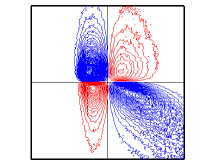
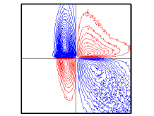
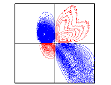
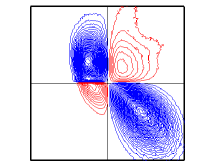
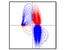
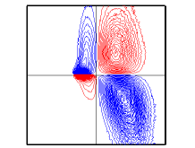
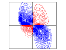
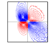
$\sigma_{2}$ $\sigma_{1}$      a)                               b)                               c)                               d) $\sigma_{2}$ $\sigma_{1}$      e)                               f)                               g)                               h)

Figure 14: The covariance integrated $q_{1}q_{2}P(q_{1},q_{2})$ at $y^{+}\approx 5$ between $u_{1}$ and $u_{2}$ with contours increments $\Delta=.00001$ a) $SM$ , b) $TS$ , c) $TT$, d) $CS$ , e) $LLS$, f) $LS$ , g) $LT$, h) $LTS$

The same behavior is observed in figure 14c for the $TT$ flow. The contours in the first quadrant have a complex shape, due to the form of the surface affecting the ejections of high intensity in the $CS$ and $TT$ surfaces. From visualizations of $\sigma_{2}$ it can be appreciated that for the corrugations with a large solid region, at the plane of the crests, the shape of the surfaces is visible up to distances $y^{+}\approx 10$. On the other hand, the surfaces are not appreciated by the $\sigma_{1}$ contours, however the elongation of the longitudinal structures is strongly reduced in particular for the $CS$ and $TT$ surfaces. In the sheet-dominated region the pdf profiles, evaluated by the joint pdf, for the $CS$ and $TT$ surfaces are symmetric for $\sigma_{2}$ and positive skewed for the $\sigma_{1}$. Due to the weak $\sigma_{2}$ disturbance in the $TS$ flow the profiles of the quadrant contributions, the covariance integrated contours in figure 14b, and the relative pdf do not change much with respect to those of the smooth surface. The $-C_{u_{1}u_{2}}$ for the surfaces with longitudinal bars are smaller in particular for the $LLS$ and the $LS$ surfaces, due to the reduction of $Q_{4}$ and the increase of $Q_{1}$. This is clearly depicted in figure 14e and figure 14f. The corresponding visualizations, not shown, emphasise the formation of very long streamwise structures with the positive streaks over the cavities and the negative over the solid. For $LLS$ the magnitude of the peaks in the layers with $\sigma_{1}>0$ is smaller than that for $LS$. The symmetric pdf of $\sigma_{2}$ do not change, instead the pdf of $\sigma_{1}$ present, for both surfaces, a sharp decrease leading to negative values of the skewness coefficient. For the $LT$ and for the $LTS$ surfaces $-C_{u_{1}u_{2}}$ increases with respect to the flows past longitudinal square bars due to the increase of the $Q_{2}$ contribution. For $LT$ the highest value of $Q_{2}$ is given in table 2; it is confirmed by the contours in figure 14g.

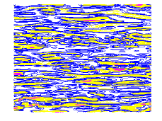
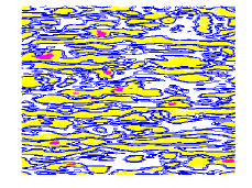
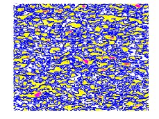
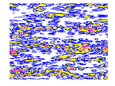
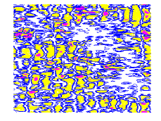
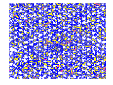
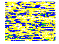
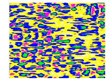
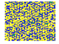
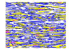
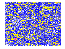
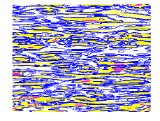
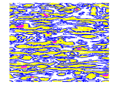
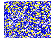
a1)                                   a2)                                   a3) b1)                                   b2)                                   b3) c1)                                   c2)                                   c3) d1)                                   d2)                                   d3) e1)                                   e2)                                   e3)

Figure 15: Contours of al) $\rho{11}$, bl) $\rho{22}$, cl) $\rho{12}$, dl) $\rho{\alpha\alpha}$, el) $\rho{\gamma\gamma}$ at $y^{+}\approx 5$ with increments $\Delta=.25$, yellow positive, blue negative for $<5$ magenta positive, for $>5$ green negative; left $SM$, center $LTS$, right $CS$.

2.2.11 Turbulent stresses visualisations

For the flows past these surfaces it is interesting to look at the flow visualizations of the stresses $u_{l}u_{m}$ in planes $x_{1}-x_{3}$ parallel to the plane of the crests. In these circumstances the stresses are evaluated by one realisation. The subscript $l$ and $m$ may indicate either the components in the Cartesian reference system or those in the frame aligned with the eigenvalues of the strain tensor $S_{ij}$. The contours in figure 15 are done for $\rho_{lm}(x_{1},x_{3})=(u_{l}u_{m}(x_{1},x_{3})-R_{lm})/R_{lm}$, with $R_{lm}=\frac{1}{N1N3}\Sigma_{N1}\Sigma_{N3}u_{l}u_{m}(x_{1},x_{3})$, at the distance $y^{+}\approx 5$ from the plane of the crests. Usually the streaks are visualised through contours of $\sigma_{1}$ producing a picture with elongated positive and negative regions similar to those in figure 15a1 for $\rho_{11}$. The yellow positive layers have few peaks with high values (magenta coloured) the less intense blue negative are located in wider elongated structures. The contours of $\rho_{22}$ in figure 15b1 depict regions of small size with a large number of intense positive values. This imply for $u_{2}$ a large flatness factor, and agrees with the covariance integrated distribution in figure 14a. In correspondence of the high values of $\rho_{22}$ high values of negative $\rho_{12}$ (green coloured) can be detected in figure 15c1. The contours of the $\rho_{\alpha\alpha}$ in figure 15d1 and of $\rho_{\gamma\gamma}$ in figure 15e1 are similar. In figure 10b $R_{\gamma\gamma}$ for $SM$ was greater than $R_{\alpha\alpha}$ in figure 10a, this difference in the visualizations can not be appreciated due to the normalisation in the expression of $\rho_{lm}$. The anisotropy of the near wall region in the Cartesian reference frame, is clearly drawn by comparing figure 15a1 and figure 15b1. In the strain rate reference system the anisotropy is visually appreciated by a comparison between the contours of $\rho_{\beta\beta}$, equal to those of $\rho_{33}$, with those in in figure 15d1 and in figure 15e1.

The figures in the central column for the $LTS$ flow of $\rho_{11}$ (figure 15a2), $\rho_{\alpha\alpha}$ (figure 15d2) and $\rho_{\gamma\gamma}$ (figure 15e2) are similar to those for $SM$, with more elongated positive regions due to the effects of the underlying surface, barely visible. On the other hand, large differences can be appreciated between the contours of $\rho_{22}$ (figure 15b2) and $\rho_{12}$ (figure 15c2) and the corresponding figure for $SM$ in the left column. For $LTS$ is clear the formation of spanwise coherent structures with intense positive peaks in correspondence of which strong negative $\rho_{12}$ appear. The common features of the $LTS$ and $SM$ surfaces is the strong influence of the $u_{2}$ fluctuations on the turbulent stress $\langle u_{1}u_{2}\rangle$ and therefore on the production of turbulence. This is a further prof that the $u_{2}$ fluctuations are those characterising wall turbulence. In presence of smooth walls the streaks do not form in particular locations. For the $LLS$ corrugations the streaks are linked to the underlying surfaces as it can be observed in visualizations, not shown for sake of brevity. The influence of the underlying surface can be appreciated in the visualizations for the $CS$ flow in the right column of figure 15. In this case the disturbances generated within the roughness layer are strong enough to destroy the near-wall anisotropy. The contours of $\rho_{11}$ (figure 15a3), $\rho_{\alpha\alpha}$ (figure 15d3) and $\rho_{\gamma\gamma}$ (figure 15e3) show that the elongated streamwise structures are not any more visible, and that their size is approximately the same as that of $\rho_{22}$. Therefore the tendency towards the isotropy in the near-wall layer is clearly depicted. In presence of strong $u_{2}$ and $u_{1}$ disturbances is found that the intense negative values of $\rho_{12}$ in figure 15c3 are strongly correlated with those of $\rho_{22}$ in figure 15b3 and also with the $\rho_{11}$. To conclude the stress distribution in the near-wall layer is strictly linked to the staggered distribution of the cubes in the corrugation.

3 Concluding remarks

This paper is focused on the connection between turbulent structures and production of turbulent kinetic energy. Emphasis has been directed towards statistics seldom considered in the analysis of wall bounded flows. Namely the full dissipation rate, the shear parameter and different expression for the production of turbulent kinetic energy. The canonical two-dimensional turbulent channel has been investigated by taking the data from DNS at high and low friction velocity Reynolds numbers. In a recent review paper Jimenez (2018) reported the debate about the eventual universality of wall bounded flows by increasing the Reynolds number. He shortly discussed the shear parameter $S^{*}$ without discussing the universality of this parameter in the near-wall region. Since $S^{+}$ does not vary with the Reynolds number, in the present paper the eddy turnover time in wall units has been evaluated by the DNS data by concluding that there is a good universality. The eddy turnover time can also be defined as the ratio between $q^{2+}$ and the full rate of dissipation $D_{k}^{+}$, in this case it has been found that it grows linearly both in the near-wall region and in the outer region, with two different constants of proportionally. Therefore there is a small layer connecting the two regions with linear growth. This result can be a first indication that the flow structures near the wall and those in the outer region are of the same kind. Those near the wall move fast and those in the outer layer slow. The linear growth near the wall is greater than that in the outer region, the passage between one and the other occurs in the layer where the $P_{k}^{+}$ sharply grows. From these data it can be, also observed that at $R_{\tau}=5200$ there is a tendency to the linear growth in the outer region. However, our view is that it will be indeed achieved by simulations at a slightly higher $Re$. From the data it was also possible to conclude that the maximum turbulent kinetic energy production scales at high Reynolds numbers and that the maximum is located at a distance from the wall where there is the transition between layers sheet-dominated and rods-dominated. Namely in the region where the ribbon unstable structures roll-up to become tubular structures. Finally it was found that the rate of isotropic dissipation largely depends on the Reynolds number, and that the full rate dissipation does not.

Flows past smooth walls have well defined boundary conditions for the velocity fields. These boundary conditions can be varied by changing the shape of the walls. Through the DNS of flows past different kind of corrugations it was observed that it is easy to increase the resistance, and rather difficult to reduce it. Drag reduction is obtained when the viscous stress at the plane of the crests reduces more than the increase of the turbulent stress $\langle u_{1}u_{2}\rangle$. In this regard it is interesting to look at the results of Arenas et al. (2018) where it is possible to get a large drag reduction by imposing $u_{2}=0$ at the plane of the crests of any kind of corrugation. In real applications this result can be achieved if someone is able to find the way to reproduce this boundary condition. Perhaps this is a very difficult task to reach, but from a mathematical point of view is important. The simulations of flows past several types of corrugations allowed to reach the conclusion that a universal behavior can not be found. However the parametrization of rough walls can be obtained through the normal to the wall stress at the plane of the crests. It was reported that the results of the DNS can give insight on the improvement of turbulence RANS closures, for instance to the Spalart-Almaras model. It was also observed that in RANS the reproduction of the turbulent kinetic energy budget is simpler by considering the full rate of dissipation instead of the isotropic rate of dissipation. The flow structures in the near-wall region for corrugations generating intense $u_{2}$ fluctuations tend to become more isotropic. For the drag reducing corrugations spanwise coherent structures forms which are easily detected by the $u_{2}$ contours and even better by pressure contours. These structures were observed at high Reynolds number by Raupach et al. (1996) in flows past canopies. They claimed that these structures were generated by inflectional velocity profiles similar to those occurring in mixing layers. In this experiment the drag is greater than that in presence of smooth walls. Similar conclusions were reached by García-Mayoral & Jiménez (2011) by simulations of flows past square bars in the case of breakdown of drag reduction and the spanwise structures were barely visualised. In the present simulations the spanwise structures were observed only in the drag reducing corrugations and it has been observed that a large role should be ascribed to the pressure. More simulations are currently performed to investigate how important are these structures.

4 Acknowledgements

We acknowledge that some of the results reported in this paper have been achieved using the PRACE Research Infrastructure resource MARCONI based at CINECA, Casalecchio di Reno, Italy. A particular thank to David Sassun helping me in the implementation of the immersed boundary method, and to Sergio Pirozzoli through a large number of discussions on wall turbulence and for the correction of the draft.

References

- Arenas et al. (2018) Arenas, I., Garcia, E., Orlandi, P., Fu, M.K., Hultmark, M. & Leonardi, S. 2018 Comparison between super-hydrophobic, liquid infused and rough surfaces: a study. submitted to Journal of Fluid Mechanics .
- Aupoix & Spalart (2003) Aupoix, B. & Spalart, P. R. 2003 Extensions of the spalart-allmaras turbulence model to account for wall roughness. International Journal of Heat and Fluid Flow 24, 454–462.
- Bernardini et al. (2014) Bernardini, M., Pirozzoli, S. & Orland, P. 2014 Velocity statistics in turbulent channel flow up to Re. Journal of Fluid Mechanics 742, 171–191.
- Burattini et al. (2008) Burattini, P., Leonardi, S., Orlandi, P. & Antonia, RA 2008 Comparison between experiments and direct numerical simulations in a channel flow with roughness on one wall. Journal of Fluid Mechanics 600, 403–426.
- Choi et al. (1993) Choi, H., Moin, P. & Kim, J. 1993 Direct numerical simulation of turbulent flow over riblets. Journal of Fluid Mechanics 255, 503–539.
- Furuya et al. (1976) Furuya, Y., Miyata & M. Fujita, H. 1976 Turbulent boundary layer and flow resistance on plates roughened by wires. J. Fluids Eng. 98, 635–644.
- García-Mayoral & Jiménez (2011) García-Mayoral, R. & Jiménez, J. 2011 Hydrodynamic stability and breakdown of the viscous regime over riblets. Journal of Fluid Mechanics 678, 317–347.
- Jimenez (2018) Jimenez, J. 2018 Coherent structures in wall-bounded turbulence. Journal of Fluid Mechanics 842, 1–100.
- Jimenez & Hoyas (2008) Jimenez, J. & Hoyas, S. 2008 Turbulent fluctuations above the buffer layer of wall-bounded flows. Journal of Fluid Mechanics 611, 215–236.
- Jiménez & Pinelli (1999) Jiménez, J. & Pinelli, A. 1999 The autonomous cycle of near–wall turbulence. J. Fluid Mech. 389, 335–359.
- Kim et al. (1987) Kim, J., Moin, P. & Moser, R. 1987 Turbulence statistics in fully developed channel flow at low reynolds number. J. Fluid Mech. 177, 133–166.
- Kline et al. (1967) Kline, S. J., Reynolds, W. C., Schraub, F. A. & Rundstadler, P. W. 1967 The structure of turbulent boundary layers. Journal of Fluid Mechanics 30, 741–773.
- Lee & Moser (2015) Lee, M. & Moser, R. D. 2015 Direct simulation of turbulent channel flow layer up to Re. Journal of Fluid Mechanics 774, 395–415.
- Lee et al. (1990) Lee, M. L., Kim, J. & Moin, P. 1990 Structure of turbulence at high shear rate. J. Fluid Mech. 216, 561–583.
- Moin & Kim (1982) Moin, P. & Kim, J. 1982 Numerical investigation of turbulent channel flow. Journal of Fluid Mechanics 118, 341–377.
- Moin & Kim (1997) Moin, P. & Kim, J. 1997 Tackling turbulence with supercomputers. Scientific American 276, 62–68.
- Nikuradse (1950) Nikuradse, J. 1950 Laws of flow in rough pipes. NACA Technical Memorandum 1292.
- Orlandi (2000) Orlandi, P. 2000 Fluid Flow Phenomena - A Numerical Toolkit. Kluwer Academic Publisher.
- Orlandi (2013) Orlandi, P. 2013 The importance of wall-normal reynolds stress in turbulent rough channel flows. Physics of Fluids 25, 110813–12.
- Orlandi et al. (2015) Orlandi, P., Bernardini, M. & Pirozzoli, S. 2015 Poiseuille and couette flows in the transitional and fully turbulent regime. Journal of Fluid Mechanics 770, 424–441.
- Orlandi & Leonardi (2006) Orlandi, P. & Leonardi, S. 2006 DNS of turbulent channel flows with two- and three-dimensional roughness. Journal of Turbulence 7 (N53).
- Orlandi et al. (2006) Orlandi, P., Leonardi, S. & Antonia, R. A. 2006 Turbulent channel with either transverse or longitudinal roughness elements on one wall. Journal of Fluid Mechanics 561, 279–305.
- Orlandi et al. (2016) Orlandi, P., Sassun, D. & S.Leonardi 2016 DNS of conjugate heat transfer in presence of rough surfaces. International Journal of Heat and Mass Transfer 100, 250–266.
- Peskin (1972) Peskin, C. S. 1972 Flow patterns around heart valves: a numerical method. J. of Comp. Phys. 25, 220–252.
- Pirozzoli et al. (2010) Pirozzoli, S., Bernardini, M. & Grasso, F. 2010 On the dynamical relevance of coherent vortical structures in turbulent boundary layers. Journal of Fluid Mechanics 648, 325–349.
- Raupach et al. (1996) Raupach, M. R., Finningan, J. J. & Brunet, Y. 1996 Coherent eddies and turbulence in vegetation canopies: the mixing layer analogy. Boundary-Layer Metereology 78, 351–386.
- Townsend (1976) Townsend, A. A. 1976 The Structure of Turbulent Shear Flows, second edition edn. Cambridge University Press.
- Tsinober (2009) Tsinober, A. 2009 An Informal Conceptual Introduction to Turbulence. Second Edition, Springer.
- Wallace (2016) Wallace, J. M. 2016 Quadrant analysis in turbulence research: history and evolution. Annual Reviews of Fluid Mechanics 48, 131–158.
- Yamamoto & Tsuji (2018) Yamamoto, Y. & Tsuji, Y. 2018 Numerical evidence of logarithmic regions in channel flow at Re. Physical Reviews Fluiids 3, 012062.