D2D Data Offloading in Vehicular Environments
with Optimal Delivery Time Selection

Abstract

Within the framework of a Device-to-Device (D2D) data offloading system for cellular networks, we propose a Content Delivery Management System (CDMS) in which the instant for transmitting a content to a requesting node, through a D2D communication, is selected to minimize the energy consumption required for transmission. The proposed system is particularly fit to highly dynamic scenarios, such as vehicular networks, where the network topology changes at a rate which is comparable with the order of magnitude of the delay tolerance. We present an analytical framework able to predict the system performance, in terms of energy consumption, using tools from the theory of point processes, validating it through simulations, and provide a thorough performance evaluation of the proposed CDMS, in terms of energy consumption and spectrum use. Our performance analysis compares the energy consumption and spectrum use obtained with the proposed scheme with the performance of two benchmark systems. The first one is a plain classic cellular scheme, the second is a D2D data offloading scheme (that we proposed in previous works) in which the D2D transmissions are performed as soon as there is a device with the required content within the maximum D2D transmission range. The results show that, in specific scenarios, the proposed scheme achieves an overall, i.e., including both cellular and D2D communications, reduction of the energy consumption of up to 70% with respect to the plain cellular scheme and of up to 18% with respect to the benchmark D2D offloading scheme. Furthermore, compared to the benchmark D2D offloading scheme in which the transmission instant is not optimized, the reduction of the energy consumed for the D2D transmissions only, is almost always above 90%, peaking at a 97% percent reduction. Regarding spectrum use, the proposed scheme allows to achieve an average fraction of the available radio resources used per control interval which ranges between 40% and 55% less than those used by the cellular scheme.

comment

1 Introduction

Device-to-Device (D2D) data offloading in cellular networks [1] is a powerful means to decrease congestion at the base stations, reduce the energy consumption of the overall system, and increase spectral efficiency. The idea is that, whenever a content is requested by a node, if the content is available at any of its neighbors, it should be obtained from it, rather than through a network infrastructure node. We define the nodes that can potentially hand the desired content to the requesting node as Potential Content Providers (PCPs). The set of PCPs depends on scenario parameters like the node density and the content popularity, and on the specific protocol design. For delay-tolerant applications, an interesting protocol design option is that, in case a node issuing a content request has no PCP in its neighborhood at the time of request, it waits for a predefined interval, known as content timeout, within which it is still possible to obtain the content from a new neighbor, encountered in the meantime [2, 3]. Only at the expiration of the content timeout, if the content has not yet been obtained, it is transmitted by the infrastructure nodes, which retrieve it from a remote source, through an Infrastructure-to-Device (I2D) transmission. This approach is particularly effective in highly dynamic scenarios, such as vehicular networks, where the network topology changes at a fast rate. The use of a content timeout allows to increase the population of PCPs beyond the set of the requesting node’s neighbors at the request time, extending such population to the nodes that will become its neighbors in the future. In this way, the system may obtain an increase of the offloading efficiency, defined as the percentage of contents delivered by using D2D communications between peer nodes (vehicles), rather than using I2D transmissions from the infrastructure nodes.

In our prior works [4, 5] we have shown that the considered type of D2D data offloading protocols are also very effective in reducing the overall energy consumption by exploiting the short-range D2D transmissions among nodes (provided that the popular contents are kept in their caches by the nodes that receive them), which require less transmit power (on average) than the conventional I2D ones performed by the eNBs. While this is true for most D2D data offloading protocols, especially when power control is in use, there is still room for a significant performance improvement, by taking full advantage of the delay tolerance of requests, with respect solution proposed in [4, 5].

Consider two nodes, and define them as neighbors if and only if their distance is less than or equal to a (nominal) maximum transmission range $r_{\max}^{\text{}}$. In previous works that follow the above described approach, in the case that, at the time of a content request, there are no PCPs within a range $d_{\max}$ from the requesting node (i.e., no neighbor has the requested content in its cache), as soon as the requesting node encounters a PCP, the content is transmitted. It is clear that, in this case, the transmission takes place at the maximum transmission range of the devices. Therefore, in a system with distance-based power control, all the requests that are not fulfilled at the request time, inherently require the use of the maximum D2D transmit power. Furthermore, in the opposite case, in which at the request time there is already a PCP, say at distance $r<r_{\max}$, the content delivery requires a transmit power that may be higher than what would be required if the delivery was postponed to a later instant, at which the involved (or any other) content provider could be closer than $r$ to the requesting node.

Motivated by this observation, in this work we propose the following approach, to define an improved Content Delivery Management System (CDMS). When a new request arrives, a controller, running, e.g., at the eNodeB (eNB), exploits knowledge of nodes positions and predicted motion in the near future (specifically, in the following content timeout window), to estimate which PCP will be in range of the requesting node in that timeframe. The content transmission is scheduled with the PCP that is predicted to be at the minimum distance from the requesting node, at the point in time when this will happen. In this way, provided that a distance-dependent transmit power control is in use, the smallest possible transmit power will be required for that content transmission. We will show that, using this approach, the energy consumption of the considered protocol for delay-tolerant application can be considerably reduced. This work extends our previous work [6], which provided preliminary simulation results regarding the energy consumption aspect. With respect to [6], in this work, we provide an analytical framework which allows to compute the statistics of the energy consumption of the proposed system, and a performance evaluation which quantifies, besides the energy consumption, also the spectrum usage of the proposed system, in comparison with a benchmark plain cellular system and with the CDMS system proposed by us in [4, 5].

The paper is organized as follows. We position our work with respect to the recent research trends in this area in Section 2. In Section 3 we describe our system model, positioning the proposed CDMS in the framework of a protocol stack tailored for D2D data offloading protocols. In Section 4 we present in detail the proposed Content Delivery Management System (CDMS) and provide an analytical framework to predict its performance. In Section 6 we describe a possible MAC (adapted from an existing solution) for an in-band implementation of the proposed D2D offloading scheme. In Section 7, through extensive system-level simulations, we validate the proposed analytical framework and evaluate the performance of the proposed system in terms of the average energy consumption per content delivery, and average spectrum use, required to satisfy a given system-wise traffic demand. Finally, Section 8 concludes the paper, summarizing our contribution and most relevant results.

2 Related work

The use of D2D communications to offload traffic from infrastructure nodes has been investigated in the recent years by the researchers of different communities. Works like [7, 8] aim at investigating scaling laws and network throughput from a fundamental limits perspective. Works like [9, 10] (amongst many others), aim at devising radio resource allocation strategies, and/or other physical layer parameters, like coding rates and transmit power levels, assuming that the D2D and/or I2D links to be scheduled are given as an input to the problem. More specific protocol-oriented works have appeared in the last years as well. The interested reader may want to check, e.g., [1] for an extensive survey. In these works, the objective is to determine and schedule I2D and D2D offloading communications as a function of the request patterns (as opposed to the above mentioned works, in which the links to be scheduled are an input to the problem). In [2], the peculiarity of D2D data offloading for delay-tolerant applications was first addressed, clarifying the advantages of offloading cellular traffic from the network infrastructure, and targeting the offloading efficiency as the key performance metric. In [3], the authors propose a basic CDMS for D2D data offloading an analyze its performance in a vehicular scenario, investigating the interplay of the content timeout duration with other system or scenario parameters, in a vehicular scenario. The presence of multiple contents with different popularity (which is related to the rate at which a specific content is requested by the devices) is not considered. In [11], in a scenario in which content delivery mostly relies on D2D-offloading, a strategy for I2D re-injection of contents in the network is proposed to mitigate the effect of temporal content starving in a certain areas. In [12], in the framework of a content dissemination problem (i.e., when contents need to reach all the nodes, without having been explicitly requested), the authors propose a mixed I2D-multicast and D2D-relaying reinforcement-learning-based strategy, which determines which users should receive the contents through D2D relaying from a neighboring device or through a direct I2D transmission. The above mentioned works, although providing interesting insights from the perspective of offloading efficiency maximization, devote less attention to performance metrics which are closer to physical quantities, like energy consumption and spectrum efficiency. Our work is motivated by the need to take into account such metrics in the system design, and optimize the design to maximize them. In [4, 5], we have elaborated a CDMS building on the one presented in [3], and proposed an analytical model to evaluate its performance [4]. In [5], we evaluate the impact, on the performance evaluation, of using different channel models, showing that simplistic scalar models models can lead to high inaccuracy when dealing with performance metrics tightly related with the physical layer aspects, like energy consumption or spectrum use. With respect to [3], our works [4, 5] take into account contents with different popularity, and considers energy consumption and spectrum occupation, besides offloading efficiency, as key performance metrics. The analytical model in [4] investigates the effect of content popularity and vehicles speed on the D2D transmit power, provides expressions for the offloading efficiency and the energy consumption of both I2D and D2D transmissions, and relies on them to select the best value for the maximum D2D transmission range. The CDMS considered in [4], however, does not optimize the D2D transmission time, letting the nodes transmit a requested content as soon as they encounter a node requesting it. In this work, differently from the above mentioned ones, we leverage the degree of freedom entailed by delay tolerance by deferring the D2D transmission instant to the time it will require the lowest power, thus achieving quite significant performance gains in terms of energy consumption. We also deem it appropriate to take into account accurate channel models, since using relatively simplistic models may result in an inaccurate estimation of the performance gain of a particular design [5]. Furthermore, we consider it necessary, when dealing with the type of performance metrics discussed above, to integrate in the performance evaluation an actual radio resource management technique. Among the many available, as done in [5], we used the solution proposed in [10], adapting it to a multi-cell scenario and to deal with frequency selective channels.

3 System model

3.1 Nodes topology, mobility, and content requests

We consider a Region of Interest (ROI) consisting of a bidirectional street chunk which vehicle enter, traverse, and exit from both ends, as shown in Fig. 1.

Vehicles enter the street according to a given stationary temporal arrival process, with an average arrival rate of $\lambda_{t}$ vehicles per second ($\lambda_{t}/2$ vehicles per second on each end). Each vehicle $n$ traverses the ROI at an average speed which is the sample of a random variable $V^{*}$ with Probability Density Function (PDF) $p_{V^{*}}(v)$. We assume that the speed value is bounded by a maximum speed $v_{\max}$. Each vehicle has onboard a mobile device, which can be either a human hand-held device or part of the vehicle equipment. Along the street, a set of eNBs is regularly placed. At each instant, each device (vehicle) is under the coverage of an eNB.

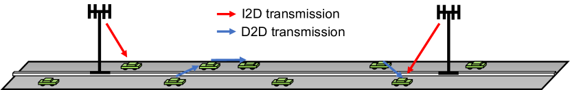
Figure 1: Sketch of the considered scenario.

Each device issues content requests according to a given stationary content request process with an average content request rate of $\lambda_{Z}$ requests per second, by sending requests messages to the eNB it is associated to at the request time. The specific content being requested is drawn from a content popularity distribution $P_{Z}(z)$. Similarly to [2, 3], we assume that the content requests can be fulfilled with some delay tolerance, i.e., they must be served at most within a content timeout $\tau_{c}$, starting at the request instant. A request may be fulfilled either by a PCP, through a D2D communication, or, if there are no PCPs, by some remote server in the Internet, using the eNB of a cellular network as the final communication hop. We assume that, in such case, the content is directly sent by an eNB. In this work we assume that, within the content timeout, the first option (delivery through D2D) is always privileged, and I2D transmissions are performed only at the end of the content timeout, if it has expired before any PCP has been found. The rationale is that, in this way, we maximize the advantage of D2D transmissions in offloading traffic from the cellular infrastructure, which is one of the primary goals of any offloading system. Furthermore, to keep the probability of cache overflow limited, each device keeps the contents it has received in its cache for a sharing timeout $\tau_{s}$, starting at the content reception instant, making it available to other nodes encountered by the device which may request it. At the expiration of the sharing timeout, to avoid an indefinite increase of the cache occupation, the content is removed from the cache. Finally, another important parameter of interest is the maximum nominal transmission range of the devices, indicated with $r_{\max}^{\text{(D2D)}}$. Table 1 summarized the basic scenario parameters introduced so far.

Table 1: Basic system model parameters

parameter	symbol
Vehicles arrival rate	$\lambda_{t}$
Vehicles speed distribution	$p_{V}\left(v\right)$
Maximum speed
Content request rate	$\lambda_{Z}$
Content popularity distribution	$P_{Z}\left(z\right)$
Content timeout	$\tau_{c}$
Sharing timeout	$\tau_{s}$
maximum nominal D2D transmission range	$r_{\max}^{\text{(D2D)}}$

The assumptions are quite general. For the purpose of performance evaluation, specific models need to be assumed for the involved random processes. We leave the description of the specific assumptions used for our performance evaluation to Section 7.

3.2 High-level view on D2D offloading control

In general, D2D-aided data offloading protocols define a strategy to handle each content request during its lifetime, from the instant it is taken in charge, to the time the content is finally delivered to the requesting node. The network infrastructure may be involved in this process in different ways. At one extreme, the whole process can be carried out autonomously by the mobile devices, typically operating out of the cellular network band, e.g. using WiFi-direct or other similar enabling communication technologies. This approach requires the frequent execution of neighbor discovery routines, and each node first seeks to obtain a content of interest directly from the neighbors, without the need of any control or support from the network infrastructure elements (such as the eNBs). Only at the approaching of the content timeout expiration, in what is sometimes called the “panic zone”, if the content has not yet been received, the node requires the content to some remote server via the cellular infrastructure. This approach has been considered, for instance, in [3].

Alternatively, as proposed in this work, the D2D-aided data offloading protocol is entirely executed under the supervision of an entity that we call Content Delivery Management System. The CDMS is a distributed software agent under the control of the network operator. Most of its functions are executed at the eNBs. Whenever a content request is generated by a user, it reaches the CDMS, which is responsible for handling it from the time it is issued by a device, until its fulfillment, deciding how and when the content request will be satisfied, either through D2D or through I2D communications. The main CDMS functions are summarized in Figure 2.

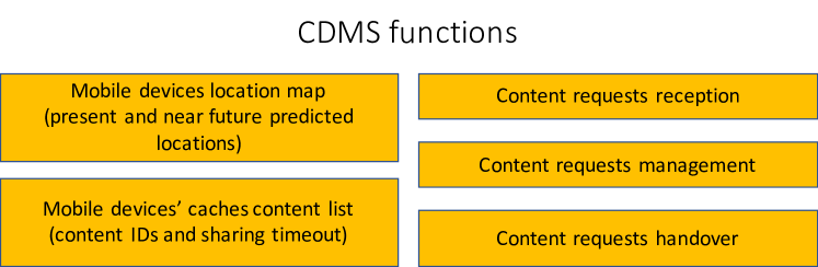
Figure 2: CDMS functions

The left column shows the two functions which provide the required information for the CDMS to operate. In general, D2D data offloading may rely on different types of information regarding the presence nodes in the region of interest, e.g., statistical (node density) or deterministic information (nodes positions). In this work, we assume that both the current nodes positions and their predicted trajectories are available. The right-hand side of Figure 2 shows the set of functions for handling the content requests. The core CDMS function is the content request management, which consists in the execution of a specific D2D offloading algorithm. The protocol decides whether a content should be provided to the requesting node by one of its neighbors or by an eNB, and at what time the transmission should be performed. In our previous works [4, 5], this protocol essentially consisted in delivering the content through D2D as soon as there is an available (i.e., within radio transmission range) PCP. In this work, we introduce a new strategy for the content provider selection, which also schedules the optimal instant and position at which the content provider is supposed to transmit the content to the requesting device. As we will show, carefully scheduling the content transmission allows to obtain a considerable performance improvement, in terms of both energy consumption and radio spectrum use. The details of the proposed protocol are described in Section 4.

In the case that a node, while waiting for a content, moves from one cell to another, the management procedure associated to that request is handed over from the eNB currently in charge of it to the adjacent one. This requires an exchange of information across adjacent eNBs.

Finally, the CDMS relies on a radio resource reuse management scheme (RRRM) which operates at the MAC layer of the cellular network protocol stack. For the purposes of this work, we have implemented a scheme that we have adapted from [10], and already used in [4, 5]. A detailed description of the considered RRRM scheme can be found in [5] and it is briefly recalled in Section 6, where we also provide details on the implementation of physical layer related aspects such as the channel model and the transmission error model. It is important to emphasize that without an accurate modeling of such aspects, it would be difficult to obtain reliable simulation results, in terms of energy consumption and spectrum use [5]. The RRRM scheme is responsible for periodically allocating the radio resources, within the time horizon of short control intervals (with duration in the order of one second) to the set of D2D and I2D content transmissions whose transmission time has been determined, with a coarser time scale, by the scheduling performed at CDMS level.

Figure 3 provides an high level abstraction of how the proposed CDMS can be implemented in a distributed way. The horizontal arrows represent the necessary exchange of information across adjacent cells. This control information flow would be typically carried out through high speed fiber connection using, e.g., the X2 interface of 4G and 5G systems. The vertical arrows represent the information provided to the RRRM component by the CDMS component.

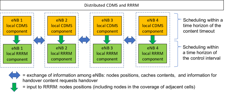
Figure 3: High level abstraction of the distributed CDMS.

4 Content Delivery Management System with optimized delivery time

For each content request it receives by the mobile devices, the CDMS executes an algorithm (explained next) which requires that it is aware of the location and expected trajectory of each node. To this end, the CDMS acts on a distributed database containing the up-to-date list of each node’s position and an estimation of their trajectories for the next $\tau_{c}$ seconds. Each device may obtain a running estimation of its speed and trajectory in the next seconds, either through the use of GPS or, if it is part of the vehicle electronic equipment, directly from the speedometer, and send it periodically to the eNBs. Alternatively, the devices can send the GPS information only to the eNB, leaving the burden of trajectory estimation to the CDMS. In general, different combinations are possible, whose details are outside the scope of this work. In this way, essentially, the CDMS has a picture of how the network topology will evolve in the next seconds. In this work, we assume a perfect prediction of the vehicles’ trajectory for an amount of time equal to the content timeout, leaving the evaluation of the robustness of the system with respect to trajectory prediction errors to a future work.

Each device $k$ has an internal content cache $\mathcal{C}_{k}$ populated with previously downloaded contents. We assume that, at any time, the CDMS also has an index of the contents in each node’s cache, and it knows the instants at which each content will be removed from the node’s cache due to the expiration of the associated sharing timeout. Each eNB keeps the above described information for all the nodes in its coverage and all the nodes in the adjacent eNBs cells, see Figure 3. The detailed actions for the execution of the proposed protocol by the CDMS are provided in Algorithm 1. Regarding the requesting node, all it does after issuing a content request is to wait for the content to be delivered to it. At the expiration of the content timeout, if it has not yet received the content by a neighboring device, it will anyway receive it from an eNB through an I2D transmission.
 

Algorithm 1 Actions taken by CDMS for handling content request $(k,z)$

1:$\mathbf{Upon}$ receiving $(k,z)$_cont_req

2:$\mathbf{set}$ $(k,z)$_served = $\mathbf{false}$

3:$\mathbf{set}$ $(k,z)$_content_timeout

4:$\mathbf{compute}$ the region of interest $\mathcal{A}^{(k,z)}$ : the area within which all PCPs can be located at the request time

5:*$\mathbf{compute}$ the set of PCPs $\mathcal{Q}_{(k,z)}=\left\{q_{1}^{(k,z)},\ldots,q_{N_{(k,z)}}^{(k,z)}\right\}$ within the area $\mathcal{A}^{(k,z)}$

6:$\mathbf{if}$ $\mathcal{Q}_{(k,z)}\neq\emptyset$

7:*  $\forall q_{i}\in\mathcal{Q}_{(k,z)}$, $\mathbf{compute}$ the optimal time and distance $t_{i}^{(k,z)}$ and $\delta_{i}^{(k,z)}$ for delivering content $z$ to device $k$ using the PCP $q_{i}$

8: $\mathbf{compute}$ $\hat{i}=\arg\min_{i\in\left\{1,\ldots,N_{(k,z)}\right\}}\left(\delta_{i}^{(k,z)}\right)$

9: $\mathbf{set}$ $\hat{\delta}^{(k,z)}:=\delta_{\hat{i}}^{(k,z)}$

10: $\mathbf{set}$ $\hat{q}^{(k,z)}:=q_{\hat{i}}^{(k,z)}$ (the selected content provider for delivering content $z$ to node $k$)

11: $\mathbf{set}$ $\hat{t}^{(k,z)}:=t_{\hat{i}}^{(k,z)}$ (the selected instant for delivering content $z$ to node $k$ using $\hat{q}^{(k,z)}$ )

12:$\mathbf{else}$

13: $\mathbf{set}$ $\hat{t}^{(k,z)}:=\tau_{c}$, $\hat{q}^{(k,z)}:=\mathbf{null}$

14:$\mathbf{end\,if}$

15:$\mathbf{while}$ $t<\hat{t}^{(k,z)}$ $\mathbf{do}$ (* the condition check is performed at every control interval)

16: $\mathbf{if}$ $\exists r\mid\boldsymbol{x}_{r}\in\mathcal{A}^{(k,z)},q\notin\mathcal{Q}_{(k,z)},\mathcal{C}_{r}\ni z$ $\mathbf{then}$

17:  $\mathbf{set}$ $q_{\text{new}}^{(k,z)}:=q$

18:  $\mathbf{compute}$ the optimal time and distance $t_{\text{new}}^{(k,z)}$ and $\delta_{\text{new}}^{(k,z)}$ for delivering using $q_{\text{new}}^{(k,z)}$

19:  $\mathbf{if}$ $\delta_{\text{new}}^{(k,z)}<\hat{\delta}^{(k,z)}$ $\mathbf{then}$

20:   $\mathbf{set}$ $\hat{q}^{(k,z)}:=q_{\text{new}}^{(k,z)}$

21:   $\mathbf{set}$ $\hat{t}^{(k,z)}:=t_{\text{new}}^{(k,z)}$

22:   $\mathbf{set}$ $\hat{\delta}^{(k,z)}:=\delta_{\text{new}}^{(k,z)}$ $\vdots$

$\hskip 39.83368pt\vdots$

23:  $\mathbf{else}$

24:   $\mathcal{R}_{(k,z)}:=\mathcal{R}_{(k,z)}\cup\left\{r\right\}$

25:   $\mathbf{discard}$ $q_{\text{new}}^{(k,z)}$, $t_{\text{new}}^{(k,z)}$, $\delta_{\text{new}}^{(k,z)}$

26:  $\mathbf{end\,if}$

27:  $\mathbf{repeat}$ steps 17-25 for each $q$ satisfying conditions at step 15

28: $\mathbf{end\,if}$

29:$\mathbf{end\,while}$

30:$\mathbf{if}$ $\hat{q}^{(k,z)}\neq\mathbf{null}$ $\mathbf{and}$ $(k,z)$_served = $\mathbf{false}$

31: $\mathbf{while}$ $t\leq\tau_{c}$

32:  $\mathbf{trigger}$ transmission $\hat{q}^{(k,z)}\stackrel{{\scriptstyle z}}{{\rightarrow}}k$

33:  $\mathbf{while}$ $(k,z)$_ACK not received

34:  $\mathbf{wait\,for}$ $(k,z)$_ACK

35:  $\mathbf{upon}$ $(k,z)$_ACK reception

36:   $\mathbf{set}$ $(k,z)$_served = $\mathbf{true}$

37:   $\mathbf{remove}$ $(k,z)$ from $\mathcal{L}_{\text{req}}$

38: $\mathbf{end\,while}$

39:$\mathbf{end\,\mathbf{if}}$

40:$\mathbf{while}$ $(k,z)$_served = $\mathbf{false}$

41: $\mathbf{send}$ $z$ to $k$ from eNB

42: $\mathbf{wait\,for}$ $(k,z)$_ACK

43: $\mathbf{upon}$ $(k,z)$_ACK reception

44:  $\mathbf{set}$ $(k,z)$_served = $\mathbf{true}$

45:  $\mathbf{remove}$ $(k,z)$ from $\mathcal{L}_{\text{req}}$

46:$\mathbf{end\,while}$

47:$\mathbf{Cancel}$ $(k,z)$_content_timeout

Essentially, on a coarse timescale, with respect to a given content request, the requesting node and the proposed CDMS act as follows. Upon receiving a content request from a node within its coverage, the eNB performs the following operations:

1. It determines the region within which PCPs for the considered request can be located. In practice, the region is determined by the maximum speed parameter $v_{\max}$, the content timeout $\tau_{c}$, and the maximum D2D transmission range $r_{\max}^{\text{(D2D)}}$. These parameters are system parameters known to the CDMS and which determine the set of PCPs that the requesting node is supposed to encounter before the content timeout for the request expires. (steps 4-5)

2. It compares the estimated trajectory of the requesting node for the next $\tau_{c}$ seconds, with those of all the nodes that have the requested content in their caches. For each PCP, it compares the expiration instant of the sharing timeout for the requested content with the expiration time of the content timeout associated to the request. If the sharing timeout will expire before the content timeout, the estimated trajectory of the PCP is considered only up to the expiration instant of the sharing timeout. (steps 6-7)

3. On the basis of the trajectories of all the PCPs, it computes (i) which provider will achieve the shortest distance from requesting device, (ii) the value of such distance, and (iii) the instant at which the two nodes are going to find themselves that close to each other. The provider with the shortest prospective distance is selected as the one who will transmit the content to the requesting node. (step 8)

4. It schedules the transmission of the content from the selected content provider to the requesting node at the time instant in which the two nodes will be at their shortest distance (compatible with the expiration of the content and sharing timeout). (steps 9-14)

5. Before the scheduled transmission instant arrives, the CDMS, with respect to the considered content request, keeps track of any device other than the selected content provider which (i) is not included in the initial set of PCPs and (ii) is supposed to encounter the requesting before the expiration of the content timeout. If any such node receives the same requested content in this period, the CDMS computes the shortest distance it will reach from the requesting node. If this new shortest distance is found to be shorter than the originally computed shortest distance, the content delivery is rescheduled to be performed by the newly found PCP, at the (new) time instant it will find itself at the newly found shortest distance. (steps 15-29)

6. At the scheduled transmit time, trigger the transmission as per the result of the assignment of the transmission to a PCP or to an eNB, and re-trigger it until an ACK is received or the content timeout expires. (steps 30-39)

7. At the expiration of the content timeout, if the content has not been received yet, transmit the content from the eNB under which the requesting device is located. (steps 40-47)

The operations described above are executed, in practice, in discrete-time, with control intervals of duration typically much lower than the content timeout. For instance, the content timeout can be in the order of one minute, and the control interval duration is in the order of 1 second. We consider a typical multi-carrier system, with control intervals determined by the organization of the radio resources onto frames, each one corresponding to a rectangular time-frequency grid of Physical Resource Blocks. For instance, considering an LTE-like MAC, a control interval could be mapped to a frame, i.e., it would last one second. The scheduled content delivery instants are hence computed in terms of number of control intervals, and mapped to the future control intervals. The content deliveries scheduled by the CDMS within the time horizon of the content timeout, will contribute, in the control interval corresponding to the prescribed delivery time, to the input to the Radio Resource Reuse (RRR) and allocation scheme described in Section 6.

5 Analytical model

In this section, we provide an analytical model for computing the statistics of the D2D transmission distance, and the associated energy consumption of mobile devices, when the CDMS described in Section 4 is in operation in the scenario described in Section 3. In the rest of this section, we represent the nodes positions in the street chunk as a unidimensional Homogeneous Spatial Poisson Point Process (HSPPP), i.e., we only consider the spatial dimension along the street median axis. For our derivations, we will use analytical results obtained in our previous paper [4], which are briefly summarized in the following Subsection 5.1. In Subsection 5.2 we compute the statistics of the D2D transmission distance resulting from the use of the proposed CDMS, and use them to compute the statistics of the associated energy consumption in Subsection 5.3. The derivations in Subsection 5.2 will follow the line of reasoning represented in Figure 4.

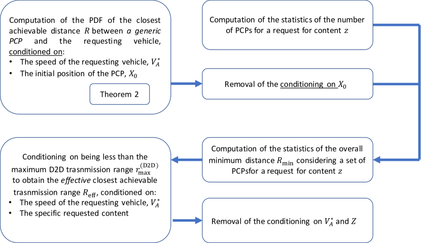
Figure 4: Summary of the derivations

Before starting, it will be useful to introduce the following notation: The symbol $p_{X}\left(\cdot\right)$ and $P_{Z}\left(\cdot\right)$ indicate the PDF and the Probability Mass Function (PMF) of continuous and discrete random variables, respectively. $F_{X}\left(\cdot\right)$ is used to represent the cumulative distribution function (CDF) of a random variable $X$, for both continuous and discrete random variables. The math blackboard expression $\mathbb{P}\left(\cdot\right)$ indicates the probability of the event enclosed in the parentheses. The function $u_{[a,b]}\left(x\right)$ represents the rectangular function defined as $u_{[a,b]}(x)=\begin{cases}1&x\in[a,b]\\ 0&x\notin[a,b]\end{cases}$. In case the domain interval is open at one or both edges, the notation $u_{(a,b]}(x)$ and $u_{(a,b)}(x)$ will be used. Setting one of the extremes to infinity, the same notation indicates the step functions equal to unity for values of $x$ larger than or equal to $a$, and zero otherwise, $u_{[a,+\infty)}(x)$, or equal to unity for values of $x$ less than or equal to $b$, and zero otherwise, $u_{(-\infty,b]}(x)$. The function $u_{0}\left(x\right)$ indicates the Dirac pulse function. The operator $\circ$ used between two functions, as in $f\left(\cdot\right)\circ g\left(\cdot\right)$, represents the convolution operator, i.e., $f\left(x\right)\circ g\left(x\right)=\smallint_{-\infty}^{\infty}f\left(x^{\prime}\right)g\left(x^{\prime}-x\right)dx^{\prime}$.

5.1 Preliminary results

Let us assume that vehicles enter the street according to a Homogeneous Temporal Poisson Point Process with a rate $\lambda_{t}$ vehicles per second (see Section 3.1) and each vehicle traverses the street at a constant speed $v$, which is independent sample of a random variable $V^{*}$ with PDF $p_{V^{*}}\left(v\right)$, and the direction of motion is incorporated in the sign of $v$. The the following hold true [4, Lemma 2]:

• The positions of the nodes along the street is a HSPPP with linear density

  $$\rho=\int_{-\infty}^{\infty}\frac{1}{\left|v\right|}\lambda_{t}p_{V^{*}}(v)dv.$$ (1)

• In the special case of uniformly distributed speeds, i.e., assuming

  $$p_{V^{*}}\left(v\right)=\frac{1}{2}\left(v_{\max}-v_{\min}\right)u_{[-v_{\max},-v_{\min}]}\left(v\right)+\frac{1}{2}\left(v_{\max}-v_{\min}\right)u_{[v_{\min},v_{\max}]}\left(v\right),$$ (2)

  the linear density of vehicles present in the street at a given instant is

  $$\rho=\lambda_{t}\left(\ln v_{\max}-\ln v_{\min}\right)/(v_{\max}-v_{\min}).$$ (3)

Furthermore, under the assumption that content requests arrive according to a HTPPP with interarrival rate $\lambda_{Z}$ and that the requested contents of different requesting nodes and across different requests are i.i.d. random variables with PMF $P_{Z}\left(z\right)$ representing the content popularity, we have that [4, Lemma 3]

• The temporal process of arrival of requests for a specific content $z$ is a HTPPP with interarrival rate

  $$\lambda_{z}=P_{Z}(z)\lambda_{Z}.$$ (4)

• The positions of nodes having content $z$ in their caches at any given time instant is a HSPPP with linear density satisfying the tight lower bound

  $$\rho_{z}\gtrsim\rho\left(1-e^{-\lambda_{z}(\tau_{s}-\tau_{c})}\right).$$ (5)

A futher result we will need is the probability that a given request is for a content that is not already cached at the device requesting it or; in other words, the probability that the request is “non-repeated”. This probability is given by $\mathbb{P}\left(\mathrm{NR}\right)=\sum_{z}P_{Z}\left(z\right)\mathbb{P}\left(\mathcal{C}\not\ni z\right)$, where $\mathcal{C}$ is the set of contents in cache of the requesting node at the request time. Finally, and the probability that the requested content is $z$, conditioned on the request being non-repeated, is given by [4, Lemma 4]

$$p_{Z}\left(z\mid\mathrm{NR}\right)=\frac{Pr\left(Z=z\right)Pr\left(\mathcal{C}\not\ni z\right)}{\sum_{z\in\mathcal{L}}Pr\left(Z=z\right)Pr\left(\mathcal{C}\not\ni z\right)}.$$ (6)

The probability that the request is non-repeated is the probability that the request fulfillment will require a transmission, either from an eNB or from a mobile device (vehicle).

5.2 Analytical model for the optimal D2D transmission distance

We start considering a device requesting a content $z$ at a given instant $t_{0}$, which is onboard a vehicle denoted with letter A, and a PCP for that request which is onboard a vehicle B. We indicate with $V_{A}^{*}$ and $V_{B}^{*}$ the random speeds at which the two vehicles are moving, and with $v_{a}^{*}$ and $v_{b}^{*}$, their respective realizations. $V_{A}^{*}$ and $V_{B}^{*}$ are i.i.d. and distributed according to a PDF $p_{V^{*}}\left(v\right)$. We incorporate the marching direction in the speed value, associating positive speed values to one direction and negative values to the opposite one. For simplicity, we assume that the absolute (i.e., unsigned) values of the speeds of vehicles marching in the two opposite directions are distributed in the same way. Since $V^{*}$ is defined as the signed speed value, this assumptions entails that $p_{V^{*}}\left(v\right)$ is symmetric around 0.

We introduce the random variable representing the relative speed between the two vehicles $V=V_{B}^{*}-V_{A}^{*}$. The PDF of the relative speed $V$, conditioned on $V_{A}^{*}$, is given by

$$p_{V\mid V_{A}^{*}}\left(v\mid v_{a}^{*}\right)=p_{V^{*}}\left(v+v_{a}^{*}\right).$$ (7)

We can assume, without loss of generality, that $v_{a}^{*}$ is positive.

Consider now the direction of motion of A and the half-line originating at A and extending in its motion direction, and assume that vehicle B is on this half-line. With the above definition of $V$ and assumption on the location of B, it holds that $v<0$ if the two vehicles are getting closer to each other, $v>0$ if their distance is increasing, and $v=0$ if the distance between the two vehicles is constant in time (since they proceed at the same speed $v^{*}$). The PDF of the relative speed between a PCP is the starting point to compute an approximate analytical expression for the PDF of the transmission range from which the eventually selected content provider will transmit the content to the requesting device. Before starting with the derivation of the approximate PDF, we first prove the following result on the maximum time limit within which a PCP should transmit the content (in case it was selected).

Lemma 1.

Consider two devices and A and B and assume that device A requests a content $z$ at $t_{0}$ and that $z$ is present in device B’s contents cache. Assume that the content timeout duration, $\tau_{c}$ is lower than the sharing timeout, $\tau_{s}$. Then the effective time limit within which vehicle B should transmit the content to the requesting device A, is a random variable $\Phi$ with the following PDF

$$p_{\Phi}\left(\phi\right)=\frac{1}{\tau_{s}}u_{[0,\tau_{c})}\left(\phi\right)+\left(1-\frac{\tau_{c}}{\tau_{s}}\right)u_{0}\left(\phi-\tau_{c}\right),$$ (8)

and average value

$$\bar{\Phi} =\tau_{c}-\frac{\tau_{c}^{2}}{2\tau_{s}}.$$ (9)

Proof 1.

Let $\Phi^{\prime}$ be a random variable representing the amount of time left, at $t=t_{0}$, before the expiration of the sharing timeout for content $z$ in vehicle B’s cache. At the expiration of the sharing timeout, the content will be deleted from vehicle B’s cache. Since the request time $t_{0}$ is independent from the time vehicle B has (previously) obtained the content, we can claim that $\Phi^{\prime}$ is uniformly distributed over the interval $[0,\tau_{s}]$, i.e., $p_{\Phi^{\prime}}\left(\phi\right)=\frac{1}{\tau_{s}}u_{[0,\tau_{s}]}\left(\phi\right)$. At the same time, the content timeout duration (which is a deterministic quantity) can be seen as a random variable whose PDF just includes a probability mass concentrated at $\tau_{c}$. To keep the same notation, indicating this variable with $\Phi^{\prime\prime}$, we have $p_{\Phi^{\prime\prime}}\left(\phi\right)=u_{0}\left(\phi-\tau_{c}\right)$. The effective time limit, within which vehicle B could transmit content $z$ to vehicle A, is determined by the first expiring timeout, among the content timeout and the sharing timeout. This time limit is, therefore, a new random variable defined as $\Phi=\min\left(\Phi^{\prime},\Phi^{\prime\prime}\right)$. It is easy to check that the corresponding PDF is given by (8). $\blacksquare$

The effective time limit is the superposition of a rectangular function of size $\tau_{c}$ weighted by $1/\tau_{s}$ and a probability mass $\left(1-\tau_{c}/\tau_{s}\right)$ concentrated at $\phi=\tau_{c}$. The first term represents the event that the sharing timeout expires before the content timeout. Its probability is given by $\tau_{c}/\tau_{s}$. If this is the case, device B will need to transmit the content before the expiration of the content timeout. The second term is the probability that the content timeout expires after the sharing timeout. In this case, device B can wait until $t=t_{0}+\tau_{c}$ to transmit the content. Note that the introduced random variable $\Phi$ represents the effective time limit within which device B can transmit the content, and not the instant at which it will eventually do so.

We now proceed with the derivation of the PDF of the closest transmission distance that a generic PCP can achieve within its time limit $\Phi$. We start considering a coordinate system still with earth, and with origin at the location of vehicle A at the request time, and indicate the random position of vehicle B at the request time with $X_{0}$. We consider now a coordinate system integral with vehicle A’s motion, with origin coincident with the (time-varying) location of vehicle A in the former coordinate system, and with the positive semi-axis of the position variable corresponding to the half-line ahead of the motion. We indicate with $x_{0}$ the realization of $X_{0}$, and observe that the position of B at the request time has the same value, $x_{0}$, in both coordinate systems. Setting, without loss of generality, $t_{0}=0$, the relative trajectory of vehicle B with respect to vehicle A is given by

$$x\left(t\right)=x_{0}+vt.$$ (10)

We indicate the best time and relative position of vehicle B, with respect to vehicle A, to eventuallyhave the PCP transmit the content the requesting device with $t^{*}$ and $x^{*}$. Given the trajectory (10), the best time and position for transmission are the those at which the distance between B and A is minimal, within the time limit $\Phi$. Intuition suggests that three cases are possible:

1. Vehicle B is moving away from vehicle A, i.e., it moves in the same direction and with an absolute speed larger than or equal to vehicle A’s speed. In this case the optimal instant and position to transmit are just $t^{*}=0$ and $x^{*}=x_{0}$, since $x(t)$ increases with time, and transmitting the content later would require more and more energy.

2. Vehicle B is either moving in the opposite direction of vehicle A’s direction, or it is moving in the same direction with a lower speed, but the two vehicles will not get to a zero distance. In this case, the optimal time and position are given by $t^{*}=\phi$ and $x^{*}=x\left(t^{*}\right)=x_{0}+v\phi$, respectively (where $\phi$ is the realization of the above defined time limit random variable $\Phi$).

3. Vehicle B is either moving in the opposite direction of vehicle A’s direction, or it is moving in the same direction with a lower speed, and the two vehicles are going to find themselves at the same location before the time limit. In this case, the optimal position is obviously $x^{*}=0$ and the optimal time is $t^{*}=-x_{0}/v$. Note that the minus sign is coherent with the convention that, for a vehicle in the half-line ahead of vehicle A’s motion, if the two vehicles are getting closer to each other, the relative speed $v$ is negative, and hence $t^{*}$ is a positive quantity.

We indicate the closest distance that the PCP can achieve from the requesting device with $R$. We indicate the PDF of $R$, conditioned on the initial position $X_{0}$ of the PCP, and on the speed $V_{A}^{*}$ of the requesting device, with $p_{R\mid X_{0},V_{A}^{*}}\left(r\mid x_{0},v_{a}^{*}\right)$, and characterize the PDF through the following

Theorem 2.

Consider a device onboard a vehicle A requesting a content $z$ at time $t_{0}$ and that $z$ is present in the cache of a device onboard a vehicle B, which is therefore a PCP for that request. Consider a unidimensional coordinate system still with earth, with origin at the position of vehicle A at the request time, and with positive axis corresponding to the motion direction of vehicle A. Let the two i.i.d. random variables $V_{A}^{*}$ and $V_{B}^{*}$, with common PDF $p_{V^{*}}\left(v^{*}\right)$, represent the absolute, signed speed of vehicle A and B, respectively, and let the relative speed of vehicle B with respect to vehicle A be defined as $V=V_{B}^{*}-V_{A}^{*}$. Let $f\left(v,v_{a}^{*}\right)\triangleq p_{V\mid V_{A}^{*}}\left(v\mid v_{a}^{*}\right)=p_{V^{*}}\left(v+v_{a}^{*}\right)$. Let $X_{0}$ denote be a random variable representing the position of vehicle B at the request time, in the so defined coordinate system. Let $R$ denote the closest distance that vehicle B can achieve, within a time limit $\Phi$ distributed as in Lemma 1.

Assume that $X_{0}$ is in the positive axis, i.e., vehicle B on the half-line ahead of vehicle A in its motion direction. Then, the PDF of $R$ can be written as

$$p_{R\mid X_{0}^{+},V_{A}^{*}}\left(r\mid x_{0},v_{a}^{*}\right)=$$ (11)

$$= +u_{(0,\infty)}\left(x_{0}\right)u_{0}\left(r-\left|x_{0}\right|\right)\int_{0}^{\infty}f\left(v,v_{a}^{*}\right)dv$$

$$+u_{(0,\infty)}\left(x_{0}\right)u_{(0,\left|x_{0}\right|)}\left(r\right)\left(\frac{1}{\tau_{s}}\int_{-\infty}^{\left(r-x_{0}\right)/\tau_{c}}f\left(v,v_{a}^{*}\right)\frac{1}{\left|v\right|}dv+\left(\frac{1}{\tau_{c}}-\frac{1}{\tau_{s}}\right)f\left(\frac{r-x_{0}}{\tau_{c}},v_{a}^{*}\right)\right)$$

$$+u_{(0,\infty)}\left(x_{0}\right)u_{0}\left(r\right)\left(\int_{-\infty}^{-x_{0}/\tau_{c}}f\left(v,v_{a}^{*}\right)dv-\frac{\left|x_{0}\right|}{\tau_{s}}\int_{-\infty}^{-x_{0}/\tau_{c}}f\left(v,v_{a}^{*}\right)\frac{1}{\left|v\right|}dv\right).$$

Assume now that $X_{0}$ is in the negative axis, i.e., vehicle B on the half-line behind vehicle A in its motion direction. Then, the PDF of $R$ can be written as

$$p_{R\mid X_{0}^{-},V_{A}^{*}}\left(r\mid x_{0},v_{a}^{*}\right)=$$ (12)

$$= u_{(-\infty,0)}\left(x_{0}\right)u_{0}\left(r-\left|x_{0}\right|\right)\int_{-\infty}^{0}f\left(v,v_{a}^{*}\right)dv$$

$$+u_{(-\infty,0)}\left(x_{0}\right)u_{(0,\left|x_{0}\right|)}\left(r\right)\left(\frac{1}{\tau_{s}}\int_{\left(\left|x_{0}\right|-r\right)/\tau_{c}}^{\infty}f\left(v,v_{a}^{*}\right)\frac{1}{\left|v\right|}dv+\left(\frac{1}{\tau_{c}}-\frac{1}{\tau_{s}}\right)f\left(\frac{\left|x_{0}\right|-r}{\tau_{c}},v_{a}^{*}\right)\right)$$

$$+u_{(-\infty,0)}\left(x_{0}\right)u_{0}\left(r\right)\left(\int_{-x_{0}/\tau_{c}}^{\infty}f\left(v,v_{a}^{*}\right)dv-\frac{\left|x_{0}\right|}{\tau_{s}}\int_{-x_{0}/\tau_{c}}^{\infty}f\left(v,v_{a}^{*}\right)\frac{1}{\left|v\right|}dv\right)$$

Finally, if the $X_{0}=0$, $R$ is deterministically equal to 0.

Overall, the PDF of $R$ is given by

$$p_{R\mid X_{0},V_{A}^{*}}\left(r\mid x_{0},v_{a}^{*}\right)= u_{(-\infty,0)}\left(x_{0}\right)p_{R\mid X_{0}^{-},V_{A}^{*}}\left(r\mid x_{0},v_{a}^{*}\right)$$ (13)

$$+u_{(0,\infty)}\left(x_{0}\right)p_{R\mid X_{0}^{+},V_{A}^{*}}\left(r\mid x_{0},v_{a}^{*}\right)+u_{0}\left(r\right)u_{0}\left(x_{0}\right)$$

Proof 2.

See Appendix A $\blacksquare$

5.2.1 Closest D2D distance from a random number of potential content providers

As described in Section 4, for each request, the CDMS computes the trajectories of a set of PCPs, and selects the best one according to the minimum of the shortest distances from the requesting device that they can achieve within their respective time limits. Such shortest distances are determined by the expiration of the content timeout (common to all) or the respective sharing timeouts (which are specific for each PCP, and distributed according to (8)).

The set of devices eligible to transmit the content is the result of the spatial point process of the positions, at the request time, of the devices that have the requested content $z$ in their caches. This process, according to our assumption, as recalled in Subsection 5.1, is a HSPPP completely characterized by its linear density, $\rho_{z}$, which is given by (5).

Let $r_{\max}^{\text{(D2D)}}$ be the maximum D2D transmission range, defined as a system parameter, and consider a coordinate system still with earth, with origin at the position of vehicle A at the request time. It is straightforward to show that

• Conditioned on $V_{A}$, a vehicle B behind vehicle A at the request time (and with the desired content in its cache) has a chance to come within a distance from vehicle A lower than or equal to the maximum transmission range $r_{\max}^{\text{(D2D)}}$ if, at the request time, it is located in the interval $[-X_{\text{$\inf$}}\left(v_{a}^{*}\right),0]$, with $X_{\text{$\inf$}}\left(v_{a}^{*}\right)=r_{\max}^{\text{(D2D)}}+\left(v_{\max}-v_{a}^{*}\right)\tau_{c}.$

• Conditioned on $V_{A}$, a vehicle B ahead of vehicle A at the request time (and with the desired content in its cache) has a chance to come within a distance from vehicle A lower than or equal to the maximum transmission range $r_{\max}^{\text{(D2D)}}$ if, at the request time, it is located in the interval $[0,X_{\sup}\left(v_{a}^{*}\right)]$, with $X_{\sup}\left(v_{a}^{*}\right)=r_{\max}^{\text{(D2D)}}+\left(v_{\max}-v_{a}^{*}\right)\tau_{c}$.

We recognize that the two spatial boundaries $X_{\text{$\inf$}}\left(v_{a}^{*}\right)$ and $X_{\sup}\left(v_{a}^{*}\right)$ have the same expression. Defining

$$X_{\text{$\lim$}}\left(v_{a}^{*}\right)\triangleq r_{\max}^{\text{(D2D)}}+\left(v_{\max}-v_{a}^{*}\right)\tau_{c},$$

we have that the street chunk corresponding to the spatial interval $[-X_{\text{$\lim$}}\left(v_{a}^{*}\right),X_{\text{$\lim$}}\left(v_{a}^{*}\right)]$ is the region in which any PCP can be located at the request time.

For the properties of HSPPPs, the initial position of the PCP in this region, $X_{0}$, conditioned on vehicle A’s speed, is uniformly distributed in the interval $[-X_{\text{$\lim$}}\left(v_{a}^{*}\right),X_{\text{$\lim$}}\left(v_{a}^{*}\right)]$, i.e.,

$$p_{X_{0}}\left(x_{0}\right)=\frac{1}{2X_{\text{$\lim$}}\left(v_{a}^{*}\right)}u_{[-X_{\text{$\lim$}}\left(v_{a}^{*}\right),X_{\text{$\lim$}}\left(v_{a}^{*}\right)]}\left(x_{0}\right).$$ (14)

Removing the conditioning on $X_{0}$ from (11), we obtain that the closest distance achievable by a PCP for a given content request, conditioned on the speed of the requesting vehicle, $V_{A}$, is distributed as

$$p_{R\mid V_{A}^{*}}\left(r\mid v_{a}^{*}\right)= \frac{1}{2X_{\text{$\lim$}}\left(v_{a}^{*}\right)}\int_{-X_{\sup}\left(v_{a}^{*}\right)}^{X_{\text{inf}}\left(v_{a}^{*}\right)}p_{R\mid X_{0},V_{A}^{*}}\left(r\mid x_{0},v_{a}^{*}\right)dx_{0},$$ (15)

where $p_{R\mid X_{0},V_{A}^{*}}\left(r\mid x_{0},v_{a}^{*}\right)$ is given by (13). Note that (15) does not depend on the specific content $z$. The specific content $z$, instead, comes into play in the following of our derivation.

Considering a content request, indicating with $Z$ the random variable representing the requested content, we can state that

Lemma 3.

The number of devices with content $z$ in their cache, positioned within the region $[-X_{\text{$\lim$}}\left(v_{a}^{*}\right),X_{\text{$\lim$}}\left(v_{a}^{*}\right)]$ centered at the position of the requesting device at the request time (i.e., the number of PCPs for that content request), a Poisson random variable $N_{\text{PCP}}\left(v_{a}^{*};z\right)$ with mean

$$\overline{N}_{\text{PCP}}\left(v_{a}^{*};z\right) =\rho_{z}2X_{\text{$\lim$}}\left(v_{a}^{*}\right)$$ (16)

and PMF

$$P_{N_{\text{PCP}}\mid V_{a}^{*},Z}\left(n\mid v_{a}^{*},z\right)=e^{-\overline{N}_{\text{PCP}}\left(v_{a}^{*};z\right)}\frac{\overline{N}_{\text{PCP}}\left(v_{a}^{*};z\right)^{n}}{n!},$$ (17)

where we have explicitly indicated the dependence on the variables $V_{A}^{*}$ and $Z$.

Proof 3.

The result comes straightforward from well known properties of homogeneous Poisson point processes. $\blacksquare$

It is worth pointing out that since the PMF, evaluated at $n=0$, is the probability that there are no PCPs in the eligibility region, it coincides with the probability that the content request will not be offloaded. Therefore, indicating the probability of offloading conditioned on a specific content $z$, and on a given speed $v_{a}^{*}$ of the vehicle with onboard the requesting device, with $\mathbb{P}\left(\text{off}\mid z,v_{a}^{*}\right)$, and the probability of sending the content using an eNB as $\mathbb{P}\left(\text{non-off}\mid z,v_{a}^{*}\right)$, we can write

$$\mathbb{P}\left(\text{non-off}\mid z,v_{a}^{*}\right) =e^{-\overline{N}_{\text{PCP}}\left(v_{a}^{*};z\right)},$$ (18a)

$$\mathbb{P}\left(\text{off}\mid z,v_{a}^{*}\right) =1-e^{-\overline{N}_{\text{PCP}}\left(v_{a}^{*};z\right)}..$$ (18b)

We now proceed by computing the best achievable transmission range resulting from the overall set of PCPs. To each PCP within the set, we can associate random variables of the kind $X_{0}$ (initial position) and $\Phi$ (PCP-specific effective time limit for eventually sending the content), resulting in two sets $X_{0}^{(1)},\ldots,X_{0}^{\left(N_{\text{PCP}}\left(v_{a}^{*};z\right)\right)}$ and $\Phi{}_{1},\ldots,\Phi{}_{N_{\text{PCP}}\left(v_{a}^{*};z\right)}$. The random variables in both sets are i.i.d. with common distribution (14) and (8), respectively. Each pair $\left[X_{0}^{(n)},\Phi{}_{n}\right],\,n\in\left\{1,\ldots,N_{\text{PCP}}\left(v_{a}^{*};z\right)\right\},$ refers to a different PCP, and determines a new random variable $R_{n}$, corresponding to the closest achievable distance of the $n$-th PCP, which, conditionally on the requesting vehicle speed, is distributed with PDF (15). By construction, the random variables in the new set $\left\{R_{1},\ldots,R_{N_{\text{PCP}}\left(v_{a}^{*};z\right)}\right\}$ are conditionally independent and identical distributed.

According to the proposed CDMS operation, the device that would eventually be selected to transmit the content to vehicle A is the one with the smallest prospective minimum distance in the set $\left\{R_{1},\ldots,R_{N_{\text{PCP}}\left(v_{a}^{*};z\right)}\right\}$. We indicate this overall minimum distance as

$$R_{\min}=\min\left(R_{1},\ldots,R_{N}\right).$$

Since the random variables $R_{1},\ldots,R_{N}$ are conditionally i.i.d., using the well known property that the CDF of the minimum among a set of i.i.d. random variables with common CDF $F\left(r\right)$ is given by $F_{\min}\left(r\right)=1-\left(1-F\left(r\right)\right)^{N},$ and introducing the conditional CDF of $R$ as

$$F_{R\mid V_{A}^{*}}\left(r\mid v_{a}^{*}\right)=\smallint_{0}^{r}p_{R\mid V_{A}^{*}}\left(r^{\prime}\mid v_{a}^{*}\right)dr^{\prime},$$

we obtain the conditional CDF of $R_{\min}$ (with conditioning random variables $V_{A}^{*}$ and $N_{\text{PCP}}\left(v_{a}^{*}/z\right)$ as

$$F_{R_{\min}\mid V_{A}^{*},\overline{N}_{\text{PCP}}\left(v_{a}^{*};z\right)}\left(r\mid v_{a}^{*},n\right)=1-\left(1-F_{R\mid V_{A}^{*}}\left(r\mid v_{a}^{*}\right)\right)^{n},$$

and the corresponding PDF as

$$p_{R_{\min}\mid V_{A}^{*},N_{\text{PCP}}\left(v_{a}^{*};z\right)}\left(r\mid v_{a}^{*},n\right) =\frac{d}{dr}F_{R_{\min}\mid V_{A}^{*},N}\left(r\mid v_{a}^{*},n\right)$$ (19)

$$=-n\left(1-F_{R\mid V_{A}^{*}}\left(r\mid v_{a}^{*}\right)\right)^{n-1}\frac{d}{dr}\left(1-F_{R\mid V_{A}^{*}}\left(r\mid v_{a}^{*}\right)\right)$$

$$=n\left(1-F_{R\mid V_{A}^{*}}\left(r\mid v_{a}^{*}\right)\right)^{n-1}p_{R\mid V_{A}^{*}}\left(r\mid v_{a}^{*}\right).$$

We now observe that, since the content will be actually delivered through a D2D transmission only if the closest distance will be lower than or equal the maximum nominal D2D transmission rage $r_{\max}^{\text{(D2D)}}$, the effective transmission distance, conditioned on $V_{A}^{*}$, results from conditioning $R_{\min}$ to being lower than or equal to $r_{\max}^{\text{(D2D)}}$. We indicate this effective transmission distance as $R_{\text{eff}}$. Its PDF is related to the PDF of the closest distance achieved by the set of PCPs (whose number, here indicated with $N$, is determined by (19)) through

$$p_{R_{\text{eff}}^{*}\mid V_{A}^{*},N,Z}\left(r\mid v_{a}^{*},n,z\right)=\frac{p_{R^{*}\mid V_{A}^{*},N,Z}\left(r\mid v_{a}^{*},n,z\right)u_{[0,r_{\max}^{\text{(D2D)}}]}\left(r\right)}{F_{R^{*}\mid V_{A}^{*},N}\left(r_{\max}^{\text{(D2D)}}\mid v_{a}^{*},n\right)},$$ (20)

where $p_{R^{*}\mid V_{A}^{*},N,Z}\left(r\mid v_{a}^{*},n,z\right)$ is given by (LABEL:subsec:D2D_distance_single_content_provider), but we have made it explicit its dependence on the specific requested content $z$, which comes into play through (16).

Combining (17) and (20), we obtain the following PDF of the effective D2D transmission distance for the considered content $z$, conditioned, now, only on $V_{A}^{*}$ and the content itself

$$p_{R_{\text{eff}}^{*}\mid V_{A}^{*},Z}\left(r\mid v_{a}^{*},z\right)=\frac{\sum_{n=1}^{\infty}P_{N_{\text{PCP}}\mid V_{a}^{*},Z}\left(n;z\right)p_{R_{\text{eff}}^{*}\mid V_{A}^{*},N_{\inf}}\left(r\mid v_{a}^{*},n\right)}{1-e^{-\bar{N}_{\text{PCP}}\left(v_{a}^{*};z\right)}}.$$ (21)

The final step to obtain the PDF of the effective D2D transmission distance $R_{\text{eff}}^{*}$ is to average out the dependency on $V_{A}^{*}$ and $Z$. In doing this, we must keep in mind that all the derivations in this section have built on the convention of taking vehicle A’s motion direction as a reference for defining the positive and negative axis of the coordinate system. Therefore, in the considered system, the speed of vehicle A is, by construction, always positive. In other words, the marginal PDF which needs to be used to compute the unconditional PDF of $R_{\text{eff}}$ for a given content $z$ is $p_{V_{A}^{*}}^{+}(v)=p_{V^{*}}(v)+p_{V^{*}}(-v)$, which, under the symmetry assumption on $p_{V^{*}}(v)$, becomes $p_{V_{A}^{*}}^{+}(v)=2p_{V^{*}}(v)$. Further removing the conditioning on the requested content $z$, we obtain the final, unconditional PDF of the optimal D2D transmission range. This result is stated in the following theorem

In conclusion, the PDF of the effective D2D transmission range for a request of content $z$ is provided by the following

Theorem 4.

Consider a content request issued by a device onboard a vehicle moving at constant (unsigned) speed which is a realization of a random variable $V_{A}^{*}$ with PDF $p_{V_{a}^{*}}^{+}(v)$, and assume that the specific requested content, $z$, is the realization of a discrete random variable $Z$ representing the content popularity, with realizations in a content library $\mathcal{Z}$ and PMF $P_{Z}\left(z\right)$. Let the assumptions on the vehicle arrival process and content request process made in Subsection 5.1 hold. Let $\rho_{z}$ be the linear density of devices with the desired content $z$ in their caches resulting from 5. Then:

• The PDF of the distance $R_{\text{eff}}$ from which the PCP that would eventually send the content to the requesting device, conditioned on the specific content $z$, is given by

  $$p_{R_{\text{eff}}\mid Z}\left(r\mid z\right) =\smallint_{0}^{\infty}p_{R_{\text{eff}}^{*}\mid V_{A}^{*},Z}\left(r\mid v_{a}^{*},z\right)p_{V_{a}^{*}}^{+}(v)dv$$ (22)

  $$=\smallint_{0}^{\infty}p_{V_{a}^{*}}^{+}(v)\sum_{n=1}^{\infty}P_{N_{\text{PCP}}\mid V_{a}^{*}}\left(n;z\right)p_{R_{\text{eff}}^{*}\mid V_{A}^{*},N_{\inf},Z}\left(r\mid v,n,z\right)dv$$

  $$=\smallint_{0}^{\infty}p_{V_{A}^{*}}^{+}(v)\sum_{n=1}^{\infty}e^{-\overline{N}_{\text{PCP}}\left(v_{a}^{*};z\right)}\frac{\overline{N}_{\text{PCP}}\left(v_{a}^{*};z\right)^{n}}{n!}p_{R_{\text{eff}}^{*}\mid V_{A}^{*},N_{\inf},Z}\left(r\mid v,n,z\right)dv$$

  with: $$\text{$\overline{N}_{\text{PCP}}\left(v_{a}^{*};z\right)$}=\rho_{z}\left(2r_{\max}^{\text{(D2D)}}+\left(v_{\max}+v_{\min}-2v_{a}^{*}\right)\tau_{c}\right),$$

  where $p_{R_{\text{eff}}^{*}\mid V_{A}^{*},N_{\text{PCP}},Z}\left(r\mid v,n,z\right)$ is given in (20).

and

• The unconditional PDF of the minimum transmission range $R_{\text{eff}}$ is

$$p_{R_{\text{eff}}}\left(r\right)= \sum_{z\in\mathcal{Z}}\left(p_{Z}\left(z\mid\mathrm{NR}\right)\int_{0}^{\infty}p_{V_{A}^{*}}^{+}\left(v_{a}^{*}\right)\vphantom{\frac{\sum_{n=1}^{\infty}P_{N_{\text{PCP}}\mid V_{a}^{*},Z}\left(n;z\right)p_{R_{\text{eff}}^{*}\mid V_{A}^{*},N_{\inf}}\left(r\mid v_{a}^{*},n\right)}{1-e^{-\overline{N}_{\text{PCP}}\left(v_{a}^{*};z\right)}}}\right.$$ (23)

$$\cdot\left.\frac{\sum_{n=1}^{\infty}P_{N_{\text{PCP}}\mid V_{a}^{*},Z}\left(n;z\right)p_{R_{\text{eff}}^{*}\mid V_{A}^{*},N_{\inf}}\left(r\mid v_{a}^{*},n\right)}{1-e^{-\overline{N}_{\text{PCP}}\left(v_{a}^{*};z\right)}}dv_{a}^{*}\right)$$

where $\mathcal{Z}$ is the content library, and $p_{Z}\left(z\mid\mathrm{NR}\right)$ is the content probability, conditioned to the fact the the content is not already in the cache of the requesting device.

Proof 4.

The two expressions of $p_{R_{\text{eff}}\mid Z}\left(r\mid z\right)$ and $p_{R_{\text{eff}}}\left(r\right)$ are simply obtained by averaging out the conditioning random variables $V_{A}^{*}$ and $Z$ from the conditional PDF (21). The denominator on the right-hand side of (23) is the probability of offloading the content, see (18b). $\blacksquare$

5.3 Analytical model for the energy consumption

To determine the energy consumption (due to the radio transmissions) induced on both the network infrastructure nodes and the devices by our CDMS, it is necessary to specify how the transmit power is set. In this work, we assume that both cellular communications (I2D) and D2D ones rely on a power control mechanism, which relates the transmit power to the distance between transmitter and receiver. More specifically, the system relies on a nominal channel gain function of transmission range, $g\left(r\right)$. Based on this function (and on standard physical layer parameters related to modulation and coding) it is able to determine the transmit power required to achieve a desired radio link reliability. More details on these aspects are provided in Section 6 and Appendix B.

We indicate with $g_{\text{I2D}}\left(r\right)$ and $g_{\text{D2D}}\left(r\right)$ two nominal channel gain functions, related to I2D and D2D transmissions, respectively, and with $\mathcal{E}\left(g\right)$ the function that relates the energy to the nominal channel gain. Furthermore, we indicate with $p_{R}^{\text{(I2D)}}(r)$ the PDF of the transmission range for the cellular tranmissions, and with $r_{\max}^{\text{(I2D)}}$ the coverage of eNBs (i.e, the cell radius). Under the assumption that the nodes positions in time are a HSPPP, using basic HSPPP properties, it is straightforward to show that $p_{R}^{\text{(I2D)}}(r)=\frac{1}{r_{\max}^{\text{(I2D)}}}u_{[0,r_{\max}^{\text{(I2D)}}]}\left(r\right)$, which does not depend on either $z$ or $v_{a}^{*}$. Thus, the average energy consumption associated to a content transmission performed by an eNB is

$$\overline{E}_{\text{I2D}}=\frac{1}{r_{\max}^{\text{(I2D)}}}\int_{0}^{r_{\max}^{\text{(I2D)}}}\mathcal{E}\left(g_{\text{I2D}}\left(r\right)\right)dr.$$ (24)

Furthermore, the probabity that a content delivery is not offloaded is given by (see (18a))

$$\mathbb{P}\left(\text{non-off}\right) =\sum_{z\in\mathcal{Z}}\left(P_{Z}\left(z\mid\text{NR}\right)\int_{0}^{\infty}\text{$\mathbb{P}\left(\text{non-off}\mid z,v_{a}^{*}\right)$}p_{V_{A}^{*}}^{+}\left(v_{a}^{*}\right)dv_{a}^{*}\right)$$ (25)

$$=\sum_{z\in\mathcal{Z}}\left(P_{Z}\left(z\mid\text{NR}\right)\int_{0}^{\infty}e^{-\overline{N}_{\text{PCP}}\left(v_{a}^{*};z\right)}p_{V_{A}^{*}}^{+}\left(v_{a}^{*}\right)dv_{a}^{*}\right),$$

For D2D trasnmissions, it is straightforward to show that

$$\overline{E}_{D2D} =\sum_{z\in\mathcal{Z}}\left(P_{Z}\left(z\mid\text{NR}\right)\int_{0}^{r_{\max}^{\text{(D2D)}}}\mathcal{E}\left(g_{\text{D2D}}\left(r\right)\right)\vphantom{\frac{\mathbb{P}\left(\text{off}\mid z,v_{a}^{*}\right)}{1-\mathbb{P}\left(\text{non-off}\right)}}\right.$$ (26)

$$\left.\int_{0}^{\infty}\frac{\mathbb{P}\left(\text{off}\mid z,v_{a}^{*}\right)}{1-\mathbb{P}\left(\text{non-off}\right)}p_{R_{\text{eff}}^{*}\mid V_{A}^{*},Z}\left(r\mid v_{a}^{*},z\right)p_{V_{A}^{*}}^{+}\left(v_{a}^{*}\right)dv_{a}^{*}dr\right)$$

where $p_{R_{\text{eff}}^{*}\mid Z}\left(r\right)$ is given by (22).

Finally, the overall average energy consumption for delivering a content is

$$\overline{E}= \mathbb{P}\left(\text{non-off}\right)\overline{E}_{\text{I2D}}+\left(1-\mathbb{P}\left(\text{non-off}\right)\right)\overline{E}_{\text{D2D}}$$ (27)

$$= \mathbb{P}\left(\text{non-off}\right)\overline{E}_{\text{I2D}}$$

$$+\int_{0}^{r_{\max}^{\text{(D2D)}}}\mathcal{E}\left(g_{\text{D2D}}\left(r\right)\right)\text{$\int_{0}^{\infty}$$\mathbb{P}\left(\text{off}\mid z,v_{a}^{*}\right)$}p_{V_{A}^{*}}^{+}\left(v_{a}^{*}\right)p_{R_{\text{eff}}^{*}\mid V_{A}^{*},Z}\left(r\mid v_{a}^{*},z\right)dv_{a}^{*}dr$$

where $p_{R_{\text{eff}}^{*}\mid V_{A}^{*},Z}\left(r\mid v_{a}^{*},z\right)$ is given by (21), $\mathbb{P}\left(\text{off}\mid z,v_{a}^{*}\right)$ by (18b), and $r_{\max}^{\text{(D2D)}}$ is the maximum transmission range of the devices.

6 MAC and physical layer implementation

In evaluating the performance of the proposed CDMS, we considered it important to use a sufficiently detailed and realistic implementation of medium access control and radio resource management layers, which takes into account the physical layer aspects that have an considerable impact on the energy consumption and interference among concurrent transmission. As shown in our recent work [5], failing to do so may result in a high degree of inaccuracy of the results. The physical layer aspects taken into account are the multipath frequency selective fading of the radio channels, spatially correlated lognormal shadowing, and interference across simultaneous transmissions. For the RRRM component, we use the same solution presented in [5], which is also compatible for being used with the CDMS proposed in this work. In the following, we summarize the main features of the RRRM component, whereas the description of the physical layer and channel models we used, the transmit power settings, and how modeled transmission errors are left to Appendix B.

We have considered a multi-carrier system in which the radio resources are organized in a time-frequency grid of Physical Resource Blocks (PRBs) of fixed bandwidth $w$ and duration $\tau$. Concurrent D2D and I2D transmissions are allowed to spatially reuse the PRBs in a very flexible way. Specifically, we have followed the approach of the resource-sharing oriented scheme proposed in [10], modifying the algorithms in [10] to use different transmit power levels across concurrent links, and including multiple eNBs and spatial frequency reuse for I2D communications (besides D2D ones) in the design, which allows to run the RRR scheme across multiple cells.

Time is organized in control intervals. In each control interval, a set of ID2 and D2D links have to be scheduled for transmission. The set of I2D and D2D links to schedule in each control interval is determined by the CDMS according to the procedure described in Section 4. Radio Resource allocation is performed by a distributed RRR agent residing at the eNBs. We assume that the position of each device is known to the RRR agent, and hence, it can compute the distance between any node pair.

The RRR agent, taking in input the distance $r$ between the transmitter and receiver of each link to be scheduled, computes the transmit power of each link. The transmit power is computed to guarantee that the channel capacity (which is a random quantity determined by fading and interference) supports the transfer of the desired amount of information with an outage probability $P_{e}\ll 1$. More details on the transmit power setting are provided in Subsection B.

The set of links is partitioned into RRR sets in order to satisfy a set of cross-interference mitigation constraints. The constraints are computed using an estimation of the interference across links obtained by computing the nominal channel gain $g$ between any link transmitter and any link receiver among the set of links to be scheduled. A suitable amount of PRBs is assigned to each RRR set. This amount is a function of the number and size of the contents that have to be transmitted by each link in the RRR set. D2D links in the same RRR set can use the same radio resources, since their belonging to the same set stands for the fact that their cross-interference is sufficiently low not to compromise the communications. I2D links originating from the same eNB are assigned radio resources in an exclusive way, selected as a portion of the pool of PRBs assigned to the RRR set they have been included in. In its portion of PRBs, however, each I2D link is subject to the interference coming from the D2D links included in the same RRR set. Finally, I2D links originating from different eNBs, that are included in the same RRR set, can be assigned the same portion of PRBs within the pool of PRBs assigned to that RRR set. If the RRR set partitioning and consequent PRBs allocation to each RRR set, due to the cross-interference constraints and to the limited number of PRBs in a control interval, prevent to accomodate the transmission of all the data required by any of the links, the data to be transmitted are pruned until reaching a feasible amount. The pruned transmissions will be rescheduled in the next control interval. Pruning is performed giving a higher scheduling priority to content deliveries related to requests whose content timeout is closer to expire. Therefore, I2D communications have a higher priority then D2D ones, since they are by design related to content requests whose timeout has already expired. If, due to pruning, the content timeout of any content request expires, the corresponding delivery is redirected to be performed by an eNB.

7 Performance evaluation

We evaluate the perfomance of the proposed CDMS using both the analytical model and simulation results. We describe the considered scenario in Subsection 7.1, and validate the theoretical model and draw some conclusions based on it in Subsection 7.2. Extensive simulations results and further comments are provided in Subsection 7.3.

7.1 Scenario description

We considered a two-lane street chunk of length 3 Km and width 20 m. The two lanes correspond to opposite marching directions. Six eNBs are placed at the horizontal coordinates of 0, 600, 1200, 1800, 2400, and 3000 m, respectively, at the center of the street (see Fig. 1). The eNB antenna height is 10 m. These numbers are in line with the “Urban Micro” scenario [13].

The distance between the median axis of the two lanes is 10 m. This is also the closest distance a vehicle can get to any vehicle marching in the opposite direction. We modeled the vehicles arrival as a HTPPP. In all the simulations whose results are, the vehicle arrival rate was kept fixed at $\lambda_{t}=1/3$ vehicles per second. Similarly, we used a HTPPP for modeling the request arrival process of each node, and kept the content request rate per device fixed at $\lambda_{Z}=1/6$ requests per second (10 requests per minute). The content requests processes of different devices were set to be statistically independent. The selected content popularity distribution was a Zipf distribution with parameter $\alpha=1.1$, i.e., $p_{Z}(z)\sim\frac{1}{\zeta(\alpha)}z^{-\alpha},$ truncated to a library size of $10^{4}$ contents. The sharing timeout was also fixed and equal to $\tau_{s}=600$ seconds. The content size was fixed and equal to a payload of 432 kB, which we assumed to be encoded in a packet of 540 kB using a FEC coding rate $\beta=0.8$. The MAC parameters we used (see Subsection 6) are as follows: each control interval lasts one second, and is divided in time slots of duration $0.5\,\text{ms}$. Each PRB lasts for 1 time slot and has width $180\,\text{KHz}$. In each PRB bandwidth, there are 12 subcarriers, the overall system bandwidth is 10.8 MHz, and in each control interval, a maximum of 120000 PRBs could be allocated to concurrent I2D and D2D transmissions (possibly spatially reusing the same PRBs across non-interfering links (see Subsection 6).

7.1.1 Simulation settings, performance metrics and benchmarks

To evaluate the performance of the proposed system, validate the analytical model, we used a custom simulator written in Matlab. The same simulator has been used for our previous works [4, 5, 6]. The simulator implements both the CDMS layer and the RRRM layer described in Sections 4 and 6, and all the considered aspects of channel, interference, and transmission error models (see Section 6 and Appendix B). More details can be found in [5].

The simulation results are organized in four different sets, each one obtained by letting a system parameter vary while keeping the rest of the parameters fixed. We focus on three parameters: the speed range $[v_{\min},v_{\max}]$ in which each vehicle’s speed falls, the content timeout $\tau_{c},$ and the maximum D2D transmission distance $r_{\max}^{\text{(D2D)}}$ (we performed two sets of simulations with varying speed range, using two different fixed values of $\tau_{c}$ and the same value for $r_{\max}^{\text{(D2D)}}$). For each value of the varying system parameter, we run 10 independent i.i.d simulations, each lasting 1 hour, reinitializing the random number generator seed with the same state at the beginning of each batch of 10 simulations. Each simulation is initialized with a random number of vehicles, positions, speeds, and cache content of each node according to the results of our previous work [4], in which we computed the steady state average number of vehicles and cache content distribution. In each simulation, we used a different independent realization of the whole set of random components of the channels between any two points in the grid, and between any eNB and any point in the grid.

We evaluate the performance of the proposed systems using the following benchmarks:

• Plain cellular system with 6 eNBs, numbered eNB1, eNB2,…, eNB6, following the order of their location. The frequency reuse pattern of length 3. The set of PRBs in each control interval is partitioned in three subsets of equal size, and each subset in the partition is assigned to the eNBs in the subsets {eNB1,eNB4}, {eNB2,eNB5}, {eNB2,eNB6}. Essentially, in each control interval, a PRB can be used exclusively by one base station within the exclusive spectrum use regions {eNB1,eNB2, eNB3}.

• CDMS presented in [4, 5], in which the D2D transmission can occur under the following circumstances:

  • Immediately after the request, if there is at least one PCP within a distance $r_{\max}^{\text{(D2D)}}$ to the requesting device. In this case, the closest PCP is selected, and the transmission distance is the same distance the two devices are from each other at the request time.

  • During the content timeout, if no PCP is within a range $r_{\max}^{\text{(D2D)}}$ to the requesting device at the request time. In this case, the first PCP which comes at a distance $r_{\max}^{\text{(D2D)}}$ to the requesting device is selected for delivering the content, and it does so at the time its being in-range is detected, therefore transmitting at the maximum distance.

The performance metrics considered in this work are

• Offloading efficiency

• Average energy consumption per content delivery, considering both I2D and D2D transmissions

• Average energy consumption per content delivered considering only D2D transmissions

• Average spectrum occupation percentage (computed an area equal to the exclusive spectrum use regions): a PRB is counted as being used if it used by at least one transmission within an exclusive spectrum use region of the cellular system. Clearly, for the benchmark cellular system, the average spectrum occupation percentage coincides with the ratio between the offered traffic and the traffic that the network is able to support without being saturated. For D2D offloading schemes, in which PRBs are spatially reused, the average spectrum occupation percentage is expected to be less.

7.2 Analytical model validation and performance trends

We validate our analytical model by comparing the statistics of the D2D transmission distance computed with it, with the sample PDF obtained in the simulations. In doing this, we also comment on the major difference, in terms of D2D transmission distance, between the proposed CDMS and the benchmark CDMS. Figure 5 shows the PDF of the D2D transmission range computed using the analytical model (solid line), and the sample PDFs obtained with the simulations running the proposed CDMS (dashed line) and the benchmark CDMS (dotted line). The system parameters are $\tau_{c}=20\text{ s}$, $r_{\max}^{\text{(D2D)}}=180\,\text{m}$, and $[v_{\min},v_{\max}]=[6,16]\,\text{m/s}$. In plotting the theoretical PDF we reintroduced the presence of the spatial dimension transversal to the street median axis. Defining $r_{y}$ as the distance between the median axes of the two street lanes, we have that the effective distance, taking into account both spatial dimensions, is given by $\widetilde{R}_{\text{eff}}=\sqrt{R_{\text{eff}}^{2}-r_{y}^{2}}$ if the selected PCP is in the opposite street lane with respect to the requesting device, and $\widetilde{R}_{\text{eff}}=R_{\text{eff}}$ otherwise. The theoretical model presents two Dirac pulses at $r=0$ and $r=10$, respectively, which account for the fraction of D2D transmissions that are performed by the PCP from the sweet spot $R_{\text{eff}}=0$, i.e., either $\widetilde{R}_{\text{eff}}=0$ or $\widetilde{R}_{\text{eff}}=r_{y}$.

It can be seen that the sample PDF closely follows the tail of the theoretical PDF, and the trends at small values of the transmission distance are similar as well. The mismatch in the area of the theoretical probability masses (which are absent from the sample PDF), is explained by the spatio-temporal sampling effect represented by the RRRM implementation. In practice, with the actual implementation of the RRRM component, the CDMS is able to determine the transmission instant ony with a precision equal to the control interval duration, which, being in the order of one second, entails a dispersion of the theoretical proability mass around an interval of few meters (depending on the speed). We can conclude that the proposed model is sufficiently accurate, since it reproduces the tail behaivor, and allows to quantify the percentage of transmissions that is performed at a very short range, e.g, less than 20 m, which is given by the overall probability mass at $R_{\text{eff}}=0$ (i.e., either $\widetilde{R}_{\text{eff}}=0$ or $\widetilde{R}_{\text{eff}}=r_{y}$).

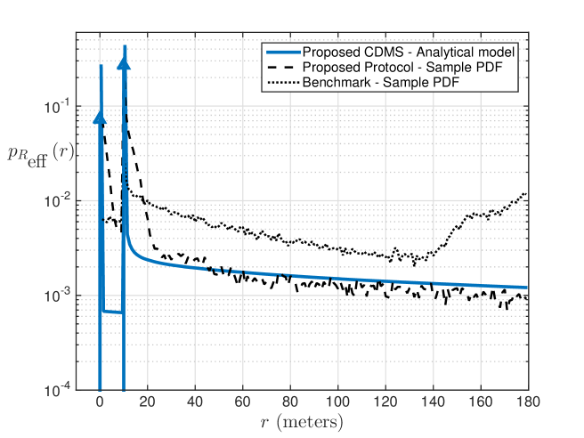
Figure 5: PDF of the D2D transmission distance $R_{\text{eff}}$

Finally, the figure also shows how much effective is the proposed CDMS in concentrating the probability mass towards short distances, with respect to the benchmark CDMS.

The surface plots in Figure 6 show the value of the probability mass at $R_{\text{eff}}=0$, i.e., the probability that the D2D transmission will be performed at very short distance (virtually equal to zero in case of PCP moving in the same direction of the requesting vehicle, and $r_{y}$ otherwise), for different values of the system parameters. We used the PDF (2). The horizontal axes correspond to speed range $[v_{\min},v_{\max}]$ and content timeout $\tau_{c}$. Different surfaces correspond to different values of $r_{\max}^{\text{(D2D)}}$, with surfaces at lower heights corresponding to higher values of $r_{\max}^{\text{(D2D)}}$, ranging from 80 to 140 m in steps of 20 m. The difference between the left and right plots is in the variation of the speed range. In the left had side surface plot, $v_{\min}$ and $v_{\max}$ are increased while keeping their difference constant, and the speeds are narrowed in a 5 m/s interval. In the right hand side, when increasing the speed range, also the difference between $v_{\max}$ and $v_{\min}$ increases.

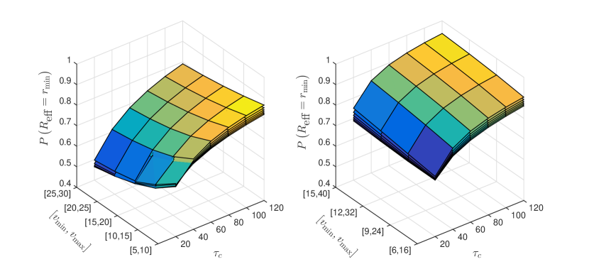
Figure 6: Probability of D2D transmission at the minimum range

From the plots we can observe that, for all configurations of speed range and maximum D2D transmission range, increasing the content timeout has a significant impact in terms of probability of transmission near the closest feasible achievable distance. Increasing the maximum transmission range $r_{\max}^{\text{(D2D)}}$ (different surfaces layered on top of each other) results in a moderate decrease of the probability of short range transmission (the height of the surfaces decreases). Finally, an interesting aspect is that, increasing $v_{\max}$ and $v_{\min}$ at the same rate (left hand side surfaces) results in a descrease of the probability of D2D transmission with the PCP close to best overall spot, whereas, increasing $v_{\max}$ while also increasing $v_{\min}$, but at a lower rate, i.e., widening the difference $v_{\min}-v_{\max}$, results in an increase of the probability of D2D trasnmission with the selected PCP close to the best place.

7.3 Simulation results and performance evaluation

In the following, we review and comment on the results of our simulations analyzing different aspects. Each figure displays a specific performance metric obtained by letting one system parameters vary, and keeping the other ones fixed. To generate the vehicles speed in inpu to the simulator, we used the PDF (2). The considered parameters are the content timeout $\tau_{c}$, the speed range $[v_{\min},v_{\max}]$, and the maximum nominal transmission range for D2D communications $r_{\max}^{\text{(D2D)}}$. The sharing timeout was set to 600 s.The remaining system parameters, kept fixed as well, are shown in Table 2.

Table 2: System parameters used for performance evaluation

System parameter	Symbol	value
Speed range	$[v_{\min},v_{\max}]$	variable
Vehicles arrival rate (new vehicles per minute)	$\lambda_{V}$	20 per minute
Node density	$\rho$	variable (see Section 5.1)
Content requests per minute (for each vehicle)	$\lambda_{C}$	6 req. per minute
Content payload size	$L$	$432\,\text{kB}$
Coded packet size	$L/\beta$	$540\,\text{kB}$
Zipf distribution parameter for the	$\alpha$	1.1
content popularity
Content timeout	$\tau_{c}$	variable
Sharing timeout	$\tau_{s}$	$600\text{ s}$
Center frequency of the system band	$f_{0}$	$2.3\text{ GHz}$
System bandwidth	$W$	$10.8\,\text{MHz}$
control interval duration	$T$	$1\text{ s}$
PRB duration	$\tau$	$0.5\,\text{ms}$
PRB bandwidth	$w$	$180\,\text{KHz}$
Number of subcarriers per PRB	$K_{sc}$	$12$
Subcarrier spacing	$w_{c}$	$15$ KHz
Noise power spectral density	$\mathcal{N}_{0}$	$-174\leavevmode\nobreak\ \text{dBm/Hz}$
Receiver noise figure	$F$	$10\,\text{dB}$
Link margin	$M$	see Section 6.2
Forward error correction coding rate	$\beta$	4/5
Transmit spectral efficiency (see Appendix )	$e$	6

7.3.1 Offloading efficiency

In Figure 7 we plot the results obtained in terms of offloading efficiency of the considered D2D offloading system (with 95% confidence intervals). The offloading efficiency tends to increase significantly with the duration of the content timeout, while varying the other parameters yields a moderate effect. Regarding the offloading efficiency of the benchmark CDMS, it can be shown that, by construction, it is the same as the proposed scheme, hence it is not showed in the figure.

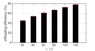
(a) With different values of $\tau_{c}$ (and fixed parameters $r_{\max}^{\text{(D2D)}}=100$ m and $[v_{\min},v_{\max}]=[9,24]$ m/s)

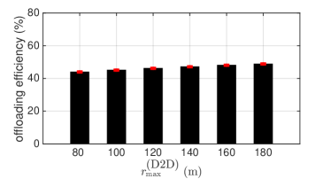
(b) With different values of $r_{\max}^{\text{(D2D)}}$ (and fixed parameters $\tau_{c}=20$ s and $[v_{\min},v_{\max}]=[9,24]$ m/s)

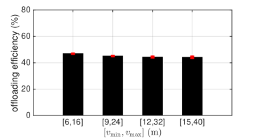
(c) With different values of $[v_{\min},v_{\max}]$ (and fixed parameters $\tau_{c}=20\text{ s}$ and $r_{\max}^{\text{(D2D)}}=100\text{ m}$)

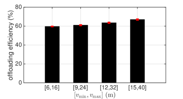
(d) With different values of $[v_{\min},v_{\max}]$ (and fixed parameters $\tau_{c}=60\text{ s}$ and $r_{\max}^{\text{(D2D)}}=100\text{ m}$)

Figure 7: Offloading efficiency

7.3.2 Energy consumption

Figure 8 shows the energy consumed on average (with confidence intervals) to deliver a content by the proposed CDMS and the plain cellular scheme. The average is performed on the overall set of both I2D and D2D transmissions (only I2D ones for the benchmark cellular scheme). It can be seen that the proposed CDMS yields a considerable improvement of this performance metric with respect to the plain cellular system. Using the proposed CDMS yields a performance gain (i.e., a reduction) of at least $13\text{ mJ}$ per content, and up to $25\text{ mJ}$, over the benchmark plain cellular protocol.

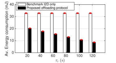
(a) With different values of $\tau_{c}$ (and fixed parameters $r_{\max}^{\text{(D2D)}}=100$ m and $[v_{\min},v_{\max}]=[9,24]$ m/s)

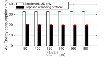
(b) With different values of $r_{\max}^{\text{(D2D)}}$ (and fixed parameters $\tau_{c}=20$ s and $[v_{\min},v_{\max}]=[9,24]$ m/s)

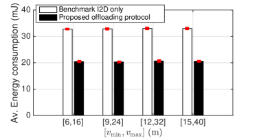
(c) With different values of $[v_{\min},v_{\max}]$ (and fixed parameters $\tau_{c}=20\text{ s}$ and $r_{\max}^{\text{(D2D)}}=100\text{ m}$)

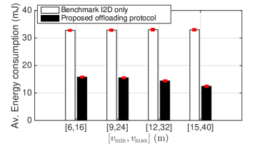
(d) With different values of $[v_{\min},v_{\max}]$ (and fixed parameters $\tau_{c}=60\text{ s}$ and $r_{\max}^{\text{(D2D)}}=100\text{ m}$)

Figure 8: Average energy consumption per delivered content

The same comparison, in terms of percentage reduction of the energy consumption, is provided in Figure 9. The reduction is in the order of 30-40% in the worst cases, up to 60% with a speed range $[15,40]\,\text{m/s}$ and a content timeout of $60\,\text{s}$ (Subfigure 9d), and 77% with a speed range of $[9,24]\,\text{m/s}$ and content timeout $20\text{ s}$.

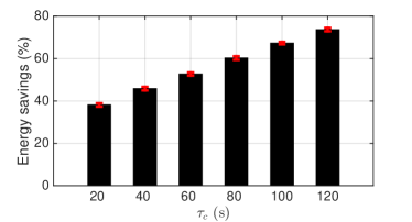
(a) With different values of $\tau_{c}$ (and fixed parameters $r_{\max}^{\text{(D2D)}}=100$ m and $[v_{\min},v_{\max}]=[9,24]$ m/s)

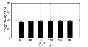
(b) With different values of $r_{\max}^{\text{(D2D)}}$ (and fixed parameters $\tau_{c}=20$ s and $[v_{\min},v_{\max}]=[9,24]$ m/s)

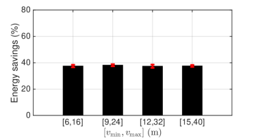
(c) With different values of $[v_{\min},v_{\max}]$ (and fixed parameters $\tau_{c}=20\text{ s}$ and $r_{\max}^{\text{(D2D)}}=100\text{ m}$)

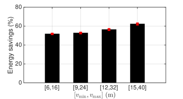
(d) With different values of $[v_{\min},v_{\max}]$ (and fixed parameters $\tau_{c}=60\text{ s}$ and $r_{\max}^{\text{(D2D)}}=100\text{ m}$)

Figure 9: Average energy consumption reduction percentage with respect to the benchmark plain cellular scheme

The performance gain relative to the benchmark D2D offloading system, still taking into account both I2D transmissions and D2D ones, is showed (with confidence intervals) in Figure 10, it can be seen that the gain ranges from a 2% reduction up to 12% (Subfigure 10.a) or 17% (Subfigure 10.b).

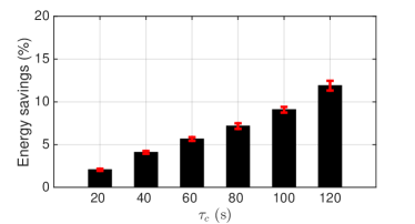
(a) With different values of $\tau_{c}$ (and fixed parameters $r_{\max}^{\text{(D2D)}}=100$ m and $[v_{\min},v_{\max}]=[9,24]$ m/s)

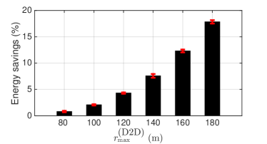
(b) With different values of $r_{\max}^{\text{(D2D)}}$ (and fixed parameters $\tau_{c}=20$ s and $[v_{\min},v_{\max}]=[9,24]$ m/s)

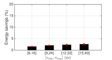
(c) With different values of $[v_{\min},v_{\max}]$ (and fixed parameters $\tau_{c}=20\text{ s}$ and $r_{\max}^{\text{(D2D)}}=100\text{ m}$)

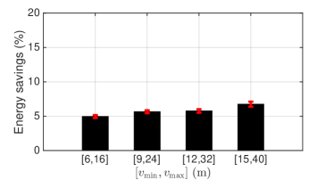
(d) With different values of $[v_{\min},v_{\max}]$ (and fixed parameters $\tau_{c}=60\text{ s}$ and $r_{\max}^{\text{(D2D)}}=100\text{ m}$)

Figure 10: System-level (I2D +D2D comms) energy consumption reduction percentage of the proposed CDMS with respect to the benchmark CDMS

Furthermore, it is worth pointing out that the overall energy consumption is dominated by the I2D component, since the energy spent for I2D communications is much larger than that spent for D2D ones, and the weights associated to the two types of communications have a comparable order of magnitude, since they are determined by the offloading efficiency, which is 80%, in the best case, among our selected configurations. Therefore, the marginal impact of the proposed CMDS cannot be fully appreciated using this performance metric. Indeed, since the mobile devices are battery powered, and the cost associated to their energy consumption impacts on the end user (while the cost of I2D communications impacts on the cellular operator), it is important to single out the gain in terms of energy consumption associated to the sole D2D communications. Figure 11 shows the average energy consumption of the benchmark D2D offloading protocol and the proposed protocol. It can be seen that the proposed protocol entails an average energy consumption, for D2D transmission, which is a small fraction of the energy spent by the benchmark protocol.

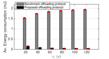
(a) With different values of $\tau_{c}$ (and fixed parameters $r_{\max}^{\text{(D2D)}}=100$ m and $[v_{\min},v_{\max}]=[9,24]$ m/s)

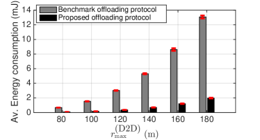
(b) With different values of $r_{\max}^{\text{(D2D)}}$ (and fixed parameters $\tau_{c}=20$ s and $[v_{\min},v_{\max}]=[9,24]$ m/s)

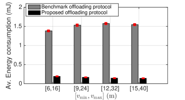
(c) With different values of $[v_{\min},v_{\max}]$ (and fixed parameters $\tau_{c}=20\text{ s}$ and $r_{\max}^{\text{(D2D)}}=100\text{ m}$)

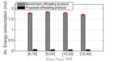
(d) With different values of $[v_{\min},v_{\max}]$ (and fixed parameters $\tau_{c}=60\text{ s}$ and $r_{\max}^{\text{(D2D)}}=100\text{ m}$)

Figure 11: Average energy consumption per delivered content, including D2D communications only - proposed CDMS and benchmark CDMS

In terms of energy consumption reduction percentage, this improvement is showed in Figure 12. For the D2D transmissions, the reduction in energy consumption is always larger than 80%, peaking at 97% in the best case (Subfigure 12.a) of content timeout equal to 120 seconds.

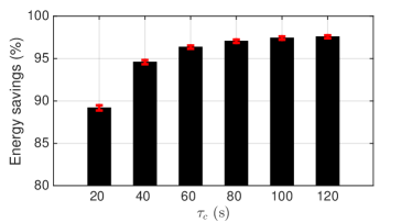
(a) With different values of $\tau_{c}$ (and fixed parameters $r_{\max}^{\text{(D2D)}}=100$ m and $[v_{\min},v_{\max}]=[9,24]$ m/s)

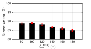
(b) With different values of $r_{\max}^{\text{(D2D)}}$ (and fixed parameters $\tau_{c}=20$ s and $[v_{\min},v_{\max}]=[9,24]$ m/s)

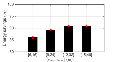
(c) With different values of $[v_{\min},v_{\max}]$ (and fixed parameters $\tau_{c}=20\text{ s}$ and $r_{\max}^{\text{(D2D)}}=100\text{ m}$)

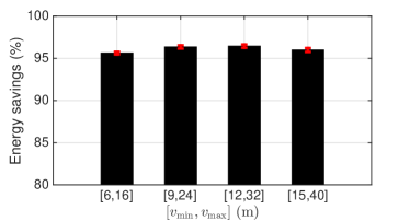
(d) With different values of $[v_{\min},v_{\max}]$ (and fixed parameters $\tau_{c}=60\text{ s}$ and $r_{\max}^{\text{(D2D)}}=100\text{ m}$)

Figure 12: Energy consumption reduction percentage of the proposed CMDS with respect to a the benchmark D2D CDMS - D2D communications only

From the analysis of the above results, it can be concluded that the most relevant parameter is the content timeout. Intuitively, if the type of data being transmitted is needed for a non time-critical application, the best thing to do, upon issuing a content request, is to wait for a while for some devices with the content passing very close to the requesting device, so that the transmission will be performed at a very short distance. The statistics of the D2D transmission distance derived in Section 5 explain why, with an increasing content timeout, the proposed protocol outperforms the benchmark one. In fact, for the benchmark protocol, increasing the content timeout increases the percentage of the D2D transmission performed with delay with respect to the request time, which (by design) are performed as soon as an encountered PCP comes at a distance equal to the maximum transmission distance, and hence using the maximum transmit power for D2D transmissions. With the proposed protocol, it is the opposite, since the PCPs have time to come very close to the requesting node.

7.3.3 Spectrum use

Figure 13 shows the average spectrum occupation percentage (with confidence intervals) of the three considered systems. The trends are similar to those observed for the energy consumption, although the proportions of absolute and relative gains are different. The offered traffic requires a spectrum occupation, for the plain cellular system, of 26% of the available radio resources, for the scenario with speed range [6,16] m/s. Increasing the speed range, the traffic load decreases, and the spectrum occupation follows the decrease (Subfigures 13.c and 13.d). The D2D offloading systems succeed in using only around 20% of the resources for the scenario with speed range [6,16] m/s, and the percentage decreases coherently with increasing speed ranges. As observable in Subfigure 13.a, and by the comparison of Subfigures 13.c and 13.d, for the spectrum use, too, the critical parameter is the content timeout. The intuitive reason is that shorter transmission distances allow for reusing the same PRBs more frequently in the spatial dimension. The D2D systems succeed in using less than 15% of the spectrum in most of the cases, dropping below 10% in the most favorable conditions of $\tau_{c}=120\,\text{s}$.

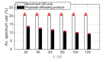
(a) With different values of $\tau_{c}$ (and fixed parameters $r_{\max}^{\text{(D2D)}}=100$ m and $[v_{\min},v_{\max}]=[9,24]$ m/s)

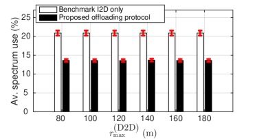
(b) With different values of $r_{\max}^{\text{(D2D)}}$ (and fixed parameters $\tau_{c}=20$ s and $[v_{\min},v_{\max}]=[9,24]$ m/s)

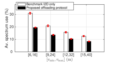
(c) With different values of $[v_{\min},v_{\max}]$ (and fixed parameters $\tau_{c}=20\text{ s}$ and $r_{\max}^{\text{(D2D)}}=100\text{ m}$)

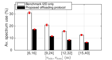
(d) With different values of $[v_{\min},v_{\max}]$ (and fixed parameters $\tau_{c}=60\text{ s}$ and $r_{\max}^{\text{(D2D)}}=100\text{ m}$)

Figure 13: Average spectrum use percentage of the benchmark protocols (plain cellular and D2D offloading) and the proposed protocol

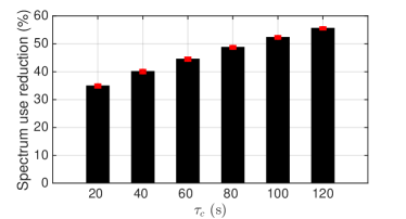
(a) With different values of $\tau_{c}$ (and fixed parameters $r_{\max}^{\text{(D2D)}}=100$ m and $[v_{\min},v_{\max}]=[9,24]$ m/s)

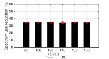
(b) With different values of $r_{\max}^{\text{(D2D)}}$ (and fixed parameters $\tau_{c}=20$ s and $[v_{\min},v_{\max}]=[9,24]$ m/s)

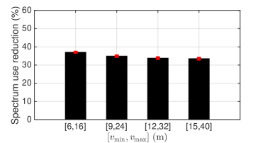
(c) With different values of $[v_{\min},v_{\max}]$ (and fixed parameters $\tau_{c}=20\text{ s}$ and $r_{\max}^{\text{(D2D)}}=100\text{ m}$)

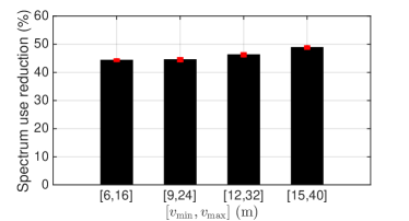
(d) With different values of $[v_{\min},v_{\max}]$ (and fixed parameters $\tau_{c}=60\text{ s}$ and $r_{\max}^{\text{(D2D)}}=100\text{ m}$)

Figure 14: Reduction percentage of the average spectrum use of the proposed CDMS with respect to the cellular system.

Figure 14 shows the percentage reduction of the spectrum occupation obtained by the D2D system (benchmark and proposed one) against the plain cellular benchmark system. The reduction is always above 30%, on average 40%, and peaking to 50% in the most favorable conditions. With respect to the benchmark system, in our simulations, we observed a reduction mostly in the range of 4 to 6%.

Commenting our results on spectrum occupation, we remark that they are closely related the specific implementation of the RRRM component we used. Particularly, one aspect that the considered RRRM does not optimize the selection of the input transmit power of the concurrent links. In fact, the transmit power is set to satisfy a constraint which is only function of the channel in the considered link. Furthermore, the considered RRRM allocates the resources to I2D and D2D links in a shared way (i.e., I2D links have no dedicated resources). It may be the case that this coexistence prevents to fully exploit the shorter D2D transmission distances achieved with the proposed scheme, thus limiting the gain in terms of spectrum use. Thus, although the reduction in spectrum use is already relevant, we believe that by using an evolved RRRM component, which optimizes the input transmit power of the concurrent links jointly, may result in a further performance improvement in terms of spatial spectrum reuse. This aspect will be considered in our future works.

8 Conclusion

We have proposed a content delivery management system for D2D data offloading in cellular networks tailored to scenarios, such as vehicular networks, where the topology varies at a fast rate, and to delay-tolerant applications. The proposed system exploits the availability of nodes mobility predictions at the CDMS. We have derived an analytical model able to predict the system performance in terms of the statistics of the D2D transmission range and the energy consumption. The analytical model allows to rapidly evaluate the system performance in a variety of scenarios larger than that allowed through system-level simulations which, with the involvement of hundreds of nodes, and the MAC and channel model implementation details, may require a very large time.

We have evaluated the system level performance using an accurate system level simulator which includes a radio resource reuse scheme for allocating resources over a time-frequency radio resource grid, and incorporates a quite detailed channel model including small scale frequency selective fading. The proposed system, in which the D2D transmission instant is selected to minimize the transmission range, allows energy savings at the system level (including I2D and D2D transmissions) ranging between 30% and 80%, depending on the scenario parameters, with respect to the benchmark cellular system, and mostly in the 5%-20% range with respect to the D2D offloading benchmark system. However, considering the sole energy consumed by the devices for operating with any of the two considered D2D offloading systems (benchmark and proposed one), the proposed system outperforms the benchmark with a reduction of around 90% of spent energy for transmission in most of the considered settings, peaking at 97% when the delay tolerance is 2 minutes, which is a reduction of almost two orders of magnitude. In terms of spectrum occupation, the proposed system uses an amount of spectrum resources (for the considered configurations) 30% to 40% less than the plain cellular system, and up to 5% less then the benchmark D2D offloading system.

We emphasize that, since the energy consumption of the devices is one of the major concerns in the evaluation of the worthiness of deploying this kind of solutions, a performance comparison in terms of the enrgy consumed by the devices, is the most appropriate, since this specific metric can make a real difference in determining if a system is worth deploying or not.

References

Appendix A Statistics of the optimal D2D transmission from a single PCP

Proof of Theorem 2 1.

To compute of the PDF of the closest distance from a device requesting a content achievable by a PCP within the time limit, it is convenient to introduce an auxiliary random variable $\Delta$ defined as the signed “displacement” of the optimal relative position of the PCP (the one at which it should transmit the content, if it was selected for doing it) with respect to its original position $X_{0}$. Coherently with this perspective, the optimal relative (i.e. referred to a coordinate system integral with vehicle A motion) position for transmission is a random variable $X^{*}=X_{0}+\Delta$. In the following, we shall use the symbols $x_{0}$ and $x^{*}$ to indicate the realizations of $X_{0}$ and $X^{*}$. We indicate the PDF of the random variable $\Delta$, conditioned on the initial position of the PCP, $X_{0}$, distinguishing between two possible cases for the conditioning realization $x_{0}$. Specifically, we use $p_{\Delta\mid X_{0}^{+},V_{A}^{*}}\left(\delta\mid x_{0}\right)$ for the case that $x_{0}>0$, and $p_{\Delta\mid X_{0}^{-},V_{A}^{*}}\left(\delta\mid x_{0},v_{a}^{*}\right)$ for the case $x_{0}<0$. The case for $x_{0}=0$ boils down to simply transmitting the content immediately, since it means that the PCP is already at the closest distance, and any delay will result in an increased distance. Accordingly, if $x_{0}=0$ the PDF of $\Delta$ is a Dirac pulse with unit mass concentrated at $r=0$.

Case for PCP ahead of requesting vehicle A: $x_{0}>0$

First of all, intuition suggest that, if $x_{0}>0$, the optimal signed displacement $\Delta$ of vehicle B (with respect to its original position $x_{0}\triangleq x\left(t_{0}\right)$) evaluated in a coordinate system integral with vehicle A’s motion, be either negative or, at most, null. Specifically, we will show that, for this case, $\Delta$ has the following properties:

• With a finite positive probability, $\Delta$ is equal to $0$, Specifically,

  $$\mathbb{P}\left(\Delta=0\mid X_{0}=x_{0},V_{A}^{*}\right)\Bigr{|}_{x_{0}>0}=\int_{0}^{\infty}f\left(v,v_{a}^{*}\right)dv.$$ (28)

• With a finite positive probability, $\Delta$ is equal to $-x_{0}$. Specifically,

  $$\small{\mathbb{P}\left(\Delta=-x_{0}\mid X_{0}=x_{0},V_{A}^{*}\right)\Bigr{|}{}_{x_{0}>0}=\int_{-\infty}^{-x_{0}/\tau_{c}}f\left(v,v_{a}^{*}\right)dv-\frac{x_{0}}{\tau_{s}}\int_{-\infty}^{-x_{0}/\tau_{c}}f\left(v,v_{a}^{*}\right)\frac{1}{\left|v\right|}dv}.$$ (29)

• For values of the realization $\delta$ in the open interval $\left(-x_{0},0\right)$, the PDF of $\Delta$ has the following expression

  $$\small{\left.p_{\Delta\mid X_{0}^{+},V_{A}^{*}}(\delta\mid x_{0},v_{a}^{*})\right|_{\delta\in(-x_{0},0)}=\frac{1}{\tau_{s}}\int_{-\tau_{c}}^{0}f\left(-\frac{\delta}{z},v_{a}^{*}\right)\frac{1}{\left|z\right|}dz+\left(\frac{1}{\tau_{c}}-\frac{1}{\tau_{s}}\right)f\left(\frac{\delta}{\tau_{c}},v_{a}^{*}\right)}$$ . (30)

In fact, consider the three cases listed on page 1. Under our assumptions, if the distance between B and A is constant or increasing (case 1 in the list), i.e., $V\geq 0$, the optimal instant for transmitting is just $t_{0}$, and hence $\Delta=0$. Therefore, the probability of having $\Delta=0$ is given by the probability that $V$ is zero or positive, as in Eq. (28). If the distance between the two vehicles is decreasing (hence, by our convention, $V<0$) but they will not achieve the same location within the expiration of either the content or they sharing timeout (case 2 in the list), the displacement (in the coordinate system integral with vehicle A) of vehicle B with respect to its original position $x_{0}$ is determined by the (relative) space travelled during an interval of duration $\Phi$. Finally, if vehicles A and B will reach the same location before the expiration of any of the timeouts (case 3 in the list), the displacement is simply given by the opposite (additive inverse) value of the original position $x_{0}$.

Summarizing, the three cases can be easily mapped to the following properties for the random variable $\Delta$:

$$\Delta=\begin{cases}0&\text{if }V\geq 0\\ V\Phi&\text{if }V<0\text{\,and\,}V\Phi>-x_{0}\\ -x_{0}&\text{if }V<0\text{\,and\,}V\Phi\leq-x_{0}\end{cases}\,.$$ (31)

Eq. (29) can be obtained through the following steps:

$$\mathbb{P}\left(\Delta=-x_{0}\right)= \mathbb{P}\left(V\Phi\leq-x_{0},V<0\right)$$

$$= \mathbb{P}\left(\Phi\geq\frac{x_{0}}{\left|V\right|},V<0\right)$$

$$= \int_{-\infty}^{0}f\left(v,v_{a}^{*}\right)\int_{x_{0}/\left|v\right|}^{\infty}p_{\Phi}(\phi)d\phi dv$$

$$= \int_{-\infty}^{0}f\left(v,v_{a}^{*}\right)\int_{x_{0}/\left|v\right|}^{\infty}\frac{1}{\tau_{s}}u_{[0,\tau_{c}]}(\phi)+\left(1-\frac{\tau_{c}}{\tau_{s}}\right)u_{0}\left(\phi-\tau_{c}\right)d\phi dv$$

$$\hphantom{\mathbb{P}\left(\Delta=-x_{0}\right)}= \int_{-\infty}^{0}f\left(v,v_{a}^{*}\right)\left(\frac{1}{\tau_{s}}\int_{x_{0}/\left|v\right|}^{\tau_{c}}d\phi\right.$$

$$\left.+\left(1-\frac{\tau_{c}}{\tau_{s}}\right)\int_{x_{0}/\left|v\right|}^{\infty}u_{0}\left(\phi-\tau_{c}\right)d\phi\right)u_{(-\infty,-x_{0}/\tau_{c}]}(v)dv$$

$$= \int_{-\infty}^{-x_{0}/\tau_{c}}f\left(v,v_{a}^{*}\right)\left(\frac{1}{\tau_{s}}\left(\tau_{c}-\frac{x_{0}}{\left|v\right|}\right)+\left(1-\frac{\tau_{c}}{\tau_{s}}\right)\right)dv$$

$$\hphantom{\mathbb{P}\left(\Delta=-x_{0}\right)}= \left(\frac{\tau_{c}}{\tau_{s}}+1-\frac{\tau_{c}}{\tau_{s}}\right)\int_{-\infty}^{-x_{0}/\tau_{c}}f\left(v,v_{a}^{*}\right)dv-\frac{x_{0}}{\tau_{s}}\int_{-\infty}^{-x_{0}/\tau_{c}}f\left(v,v_{a}^{*}\right)\frac{1}{\left|v\right|}dv$$

$$= \int_{-\infty}^{-x_{0}/\tau_{c}}f\left(v,v_{a}^{*}\right)dv-\frac{x_{0}}{\tau_{s}}\int_{-\infty}^{-x_{0}/\tau_{c}}f\left(v,v_{a}^{*}\right)\frac{1}{\left|v\right|}dv.$$

Eq. (30), which refers to the case for negative relative speed values (vehicles getting closer to each other), but not sufficiently large to let vehicle B reach vehicle A, is derived as follows. Let us indicate the CDF of $\Delta$ as $F_{\Delta}(\delta)\triangleq\mathbb{P}\left(\Delta\leq\delta\right)$, then we have

$$\left.F_{\Delta}(\delta)\right|_{\delta\in(-x_{0},0)}= \left.\mathbb{P}\left(\Delta\leq\delta\right)\right|_{\delta\in(-x_{0},0)}$$

$$= \mathbb{P}\left(V\Phi\leq-x_{0},V<0\right)+\mathbb{P}\left(-x_{0}<V\Phi\leq\delta,V<0\right)$$

$$\mathbb{P}\left(\Delta=-x_{0}\right)+\mathbb{P}\left(-x_{0}<V\Phi\leq\delta,V<0\right)$$

$$= \mathbb{P}\left(\Delta=-x_{0}\right)+\mathbb{P}\left(\frac{\delta}{V}<\Phi\leq\frac{-x_{0}}{V},V<0\right)$$

$$= \mathbb{P}\left(\Delta=-x_{0}\right)+\int_{-\infty}^{0}f\left(v,v_{a}^{*}\right)\int_{\delta/v}^{-x_{0}/v}p_{\Phi}(\phi)d\phi dv$$

Taking the derivative of $F_{\Delta}(\delta)$ with respect to $\delta$ we obtain

$$\left.p_{\Delta}(\delta)\right|_{\delta\in(-x_{0},0)}= \frac{d}{d\delta}\left.F_{\Delta}(\delta)\right|_{\delta\in(-x_{0},0)}$$

$$= \int_{-\infty}^{0}f\left(v,v_{a}^{*}\right)\frac{d}{d\delta}\int_{\delta/v}^{-x_{0}/v}p_{\Phi}(\phi)d\phi dv$$

$$= \int_{-\infty}^{0}f\left(v,v_{a}^{*}\right)\frac{1}{v}\frac{d}{d(\delta/v)}\left(\int_{\delta/v}^{-x_{0}/v}p_{\Phi}\left(\phi\right)d\phi\right)dv$$

$$= \int_{-\infty}^{0}f\left(v,v_{a}^{*}\right)\frac{1}{v}(-1)p_{\Phi}\left(\delta/v\right)dv$$

$$\hphantom{\left.p_{\Delta}(\delta)\right|_{\delta\in(-x_{0},0)}}= \int_{-\infty}^{0}f\left(v,v_{a}^{*}\right)\frac{1}{\left|v\right|}\left(\frac{1}{\tau_{s}}u_{[0,\tau_{c}]}\left(\frac{\delta}{v}\right)+\left(1-\frac{\tau_{c}}{\tau_{s}}\right)u_{0}\left(\frac{\delta}{v}-\tau_{c}\right)\right)dv$$

$$\frac{1}{\tau_{s}}\int_{-\infty}^{\delta/\tau_{c}}f\left(v,v_{a}^{*}\right)\frac{1}{\left|v\right|}dv$$

$$+\left(1-\frac{\tau_{c}}{\tau_{s}}\right)\int_{-\infty}^{0}f\left(v,v_{a}^{*}\right)\frac{1}{\left|v\right|}u_{0}\left(\frac{\delta}{v}-\tau_{c}\right)dv$$

$$= \frac{1}{\tau_{s}}\int_{-\infty}^{\delta/\tau_{c}}p_{V}(v)\frac{1}{\left|v\right|}dv$$

$$+\left(1-\frac{\tau_{c}}{\tau_{s}}\right)\int_{0}^{-\infty}f\left(-\frac{\delta}{z},v_{a}^{*}\right)\left|\frac{z}{\delta}\right|u_{0}\left(-z-\tau_{c}\right)\frac{\delta}{z^{2}}dz$$

$$= \frac{1}{\tau_{s}}\int_{-\infty}^{\delta/\tau_{c}}f\left(v,v_{a}^{*}\right)\frac{1}{\left|v\right|}dv$$

$$+\left(1-\frac{\tau_{c}}{\tau_{s}}\right)(-1)\int_{-\infty}^{0}f\left(-\frac{\delta}{z},v_{a}^{*}\right)\left(-\frac{1}{\left|z\right|}\right)u_{0}\left(z+\tau_{c}\right)dz$$

$$\vdots$$

$$\vdots$$

$$= \frac{1}{\tau_{s}}\int_{-\infty}^{\delta/\tau_{c}}f\left(v,v_{a}^{*}\right)\frac{1}{\left|v\right|}dv+\left(1-\frac{\tau_{c}}{\tau_{s}}\right)p_{V}\left(\frac{\delta}{\tau_{c}}\right)\frac{1}{\tau_{c}}$$

$$= \frac{1}{\tau_{s}}\int_{-\infty}^{\delta/\tau_{c}}f\left(v,v_{a}^{*}\right)\frac{1}{\left|v\right|}dv+\left(\frac{1}{\tau_{c}}-\frac{1}{\tau_{s}}\right)p_{V}\left(\frac{\delta}{\tau_{c}}\right)$$

$$\hphantom{\left.p_{\Delta}(\delta)\right|_{\delta\in(-x_{0},0)}}= \frac{1}{\tau_{s}}\int_{-\infty}^{0}f\left(v,v_{a}^{*}\right)\frac{1}{\left|v\right|}u_{(-\infty,\delta/\tau_{c}]}\left(v\right)dv$$

$$+\left(1-\frac{\tau_{c}}{\tau_{s}}\right)\int_{-\infty}^{0}f\left(v,v_{a}^{*}\right)\frac{1}{\left|v\right|}u_{0}\left(\frac{\delta}{v}-\tau_{c}\right)dv$$

$$\hphantom{\left.p_{\Delta}(\delta)\right|_{\delta\in(-x_{0},0)}}= \frac{1}{\tau_{s}}\int_{-\infty}^{\delta/\tau_{c}}f\left(v,v_{a}^{*}\right)\frac{1}{\left|v\right|}dv$$

$$+\left(1-\frac{\tau_{c}}{\tau_{s}}\right)\int_{0}^{\infty}f\left(\frac{\delta}{z},v_{a}^{*}\right)\left|\frac{z}{\delta}\right|\left(-\frac{\delta}{z^{2}}\right)u_{0}\left(z-\tau_{c}\right)dz$$

$$\hphantom{\left.p_{\Delta}(\delta)\right|_{\delta\in(-x_{0},0)}}= \frac{1}{\tau_{s}}\int_{-\infty}^{\delta/\tau_{c}}f\left(v,v_{a}^{*}\right)\frac{1}{\left|v\right|}dv$$

$$+\left(1-\frac{\tau_{c}}{\tau_{s}}\right)\int_{0}^{\infty}f\left(\frac{\delta}{z},v_{a}^{*}\right)\left|\frac{1}{z}\right|u_{0}\left(z-\tau_{c}\right)dz$$

$$= \frac{1}{\tau_{s}}\int_{-\infty}^{\delta/\tau_{c}}f\left(v,v_{a}^{*}\right)\frac{1}{\left|v\right|}dv+\left(1-\frac{\tau_{c}}{\tau_{s}}\right)f\left(\frac{\delta}{\tau_{c}},v_{a}^{*}\right)\frac{1}{\tau_{c}}$$

$$= \frac{1}{\tau_{s}}\int_{-\infty}^{\delta/\tau_{c}}f\left(v,v_{a}^{*}\right)\frac{1}{\left|v\right|}dv+\left(\frac{1}{\tau_{c}}-\frac{1}{\tau_{s}}\right)f\left(\frac{\delta}{\tau_{c}},v_{a}^{*}\right).$$

Combining the Eq. (28) through (30), we obtain

$$p_{\Delta\mid X_{0}^{+},V_{A}^{*}}\left(\delta\mid x_{0},v_{a}^{*}\right)=$$ (32)

$$= u_{0}\left(\delta+x_{0}\right)\left(\int_{-\infty}^{-x_{0}/\tau_{c}}f\left(v,v_{a}^{*}\right)dv-\frac{x_{0}}{\tau_{s}}\int_{-\infty}^{-x_{0}/\tau_{c}}f\left(v,v_{a}^{*}\right)\frac{1}{\left|v\right|}dv\right)$$

$$+u_{(-x_{0},0)}\left(\delta\right)\left(\frac{1}{\tau_{s}}\int_{-\infty}^{\delta/\tau_{c}}f\left(v,v_{a}^{*}\right)\frac{1}{\left|v\right|}dv+\left(\frac{1}{\tau_{c}}-\frac{1}{\tau_{s}}\right)f\left(\frac{\delta}{\tau_{c}},v_{a}^{*}\right)\right)$$

$$+u_{0}\left(\delta\right)\int_{0}^{\infty}f\left(v,v_{a}^{*}\right)dv$$

which is easy to compute, either analytically or numerically, once a specific PDF for the relative speed $V$, $f\left(v,v_{a}^{*}\right)$, is specified.

We observe that, in the case (considered above) that vehicle B is in the half-line ahead of vehicle A’s motion, the signed displacement $\Delta$ can take either negative or null values, whereas the original position of vehicle B, $x_{0}$, and its trajectory in the coordinate system integral with vehicles A’s motion, (10), always take positive or null values. Therefore, the expression of the trajectory also gives the distance between the two vehicles across time. The same holds for the optimal position $X^{*}=X_{0}+\Delta$, which, in the case $x_{0}>0$, coincides with the optimal D2D transmission distance.

Case for PCP behind the requesting vehicle A: $x_{0}<0$

Considering, now, the case that vehicle B is in the half-line behind vehicle A’s motion, we have that $X_{0}$ and $X^{*}$ can only take negative or null values, and the signed displacement $\Delta$ can only take either positive or null values. Furthermore (see footnote 2), $v>0$ if the vehicles are getting closer to each other, and $v<0$ if they are getting farther. Using a line of reasoning similar to the one used above, we obtain that, in function of the realization $x_{0}$ of the original position of vehicle B $X_{0}$,

$$\Delta=\begin{cases}0&\text{if }V\leq 0\\ V\Phi&\text{if }V>0\text{\,and\,}V\Phi<\left|x_{0}\right|\\ -x_{0}&\text{if }V>0\text{\,and\,}V\Phi\geq\left|x_{0}\right|\end{cases}\,.$$ (33)

In this case, however, the optimal D2D transmission distance is given by the opposite of the (now negative) optimal relative position $X^{*}$. With derivations similar to those presented in Appendix A, the following expression can be obtained for the displacement in the case that vehicle B, at the request time, lies on the half-line behind vehicle A:

$$p_{\Delta\mid X_{0}^{-},V_{A}^{*}}\left(\delta\mid x_{0},v_{a}^{*}\right)=$$ (34)

$$= u_{0}\left(\delta\right)\int_{-\infty}^{0}f\left(v,v_{a}^{*}\right)dv$$

$$+u_{(0,-x_{0})}\left(\delta\right)\left(\frac{1}{\tau_{s}}\int_{\delta/\tau_{c}}^{\infty}f\left(v,v_{a}^{*}\right)\frac{1}{\left|v\right|}dv+\left(\frac{1}{\tau_{c}}-\frac{1}{\tau_{s}}\right)f\left(\frac{\delta}{\tau_{c}},v_{a}^{*}\right)\right)$$

$$+u_{0}\left(\delta+x_{0}\right)\left(\int_{-x_{0}/\tau_{c}}^{\infty}f\left(v,v_{a}^{*}\right)dv-\frac{\left|x_{0}\right|}{\tau_{s}}\int_{-x_{0}/\tau_{c}}^{\infty}f\left(v,v_{a}^{*}\right)\frac{1}{\left|v\right|}dv\right).$$

Minimal distance between the two vehicles within the effective time limit

Now, the relationship of the variable $R$ with $\Delta$ can be summarized as follows.

$$R =\Bigl{|}X_{0}\Bigr{|}-\Bigl{|}\Delta\Bigr{|}=\begin{cases}X_{0}+\Delta&\text{if\,}X_{0}>0\\ 0&\text{if\,}X_{0}=0\\ -X_{0}-\Delta&\text{if\,}X_{0}<0\end{cases}\,.$$ (35)

Replacing $\delta$, in (32) and (34), with the corresponding value of the realization, $r$, of $R$, i.e., $\delta=\begin{cases}r-x_{0}&\text{if }x_{0}>0\\ x_{0}-r&\text{if }x_{0}<0\end{cases}$, we obtain (11) and (12) which, including the unitary probability mass at $r=0$ when $x_{0}=0$, combine to provide the desired expression (13) of the conditional PDF of the closest achievable transmission distance for the PCP. $\blacksquare$

Appendix B Physical layer model, transmit power setting, and packet error modeling

In the majority of network level studies, the radio channel between any two transceivers is represented as a scalar quantity, namely an attenuation coefficient, which allows a simple mapping between the signal to noise ratio (SNR) and the packet error probability. This approach, however, may result in a considerable accuracy when dealing with a multicarrier wideband system, in which channels are subject to frequency selective fading and lognormal shadowing, with spatially correlated statistic parameters [13]. Using simplistic channels may lead to a considerable inaccuracy in the evaluation of the transmit power required for a successful transmission. In this work, rather than the SNR, to compute the required transmit power we use the approach of guaranteeing a prescribed outage probability on the Shannon capacity of the channel, referred to a nominal bandwidth. More precisely, let $f$ be the frequency and $H(f)$ be the channel frequency response We assume that power is allocated uniformly over the subcarriers in use and indicate with $\mathcal{P}_{c}$ the transmit power used on each subcarrier in use. Let $\sigma_{c}^{2}=\digamma_{\text{noise}}\mathcal{N}_{0}w_{c}$ is the noise power on a subcarrier bandwidth, where $\mathcal{N}_{0}$ is the thermal noise spectral density, $\digamma_{\text{noise}}$ is the receiver noise figure, and $w_{c}$ is the subcarrier bandwidth. The Shannon capacity of the portion of spectrum corresponding to subcarrier $k$ of the channel of a radio link of interest, is given by

$$c_{k}=w_{c}\log_{2}\left(1+\mathcal{P}_{c}\left|H(f_{k})\right|^{2}/\left(\sigma_{c}^{2}+\sum_{i=1}^{S}\mathcal{P}_{c}^{(i)}\left|H_{i}(f_{k})\right|^{2}\right)\right),$$

where the index $i$ runs over the, say, $S$ interfering transmitters, and $H_{i}(f_{k})$ is the transfer function, evaluated at $f_{k}$, the $i$-th interfering transmitter and the receiver of the radio link of interest, and $\mathcal{P}_{c}^{(i)}$ is the transmit power of the $i$-th interfering transmitter. The achievable amount of information that can be transferred, in an information theoretic sense, using a PRB, is $I_{\text{PRB}}=\tau\sum_{k=1}^{K_{sc}}c_{k}$, where $K_{sc}$ is the number of subcarriers in a PRB bandwidth. Assuming that, on each subcarrier, a fixed modulation scheme is used, in which $e$ bits are encoded in a symbol (e.g., a 64QAM constellation allows to encode $e=6$ bps/Hz), the maximum achievable rate on a subcarrier is limited by $\bar{c}_{k}=\min$$\left(c_{k},ew_{c}\right)$.

We set the transmit power per subcarrier $\mathcal{P}_{c}$ for transmitting over a range $r$, as a function of the nominal channel gain $g\left(r\right)$. More precisely, we find the power required to support a capacity equal the information rate $ew_{c}$ required by the constellation in use, and, to compensate for the effect of fading and (eventual) interference, we add a suitable link margin. More specifically, we invert the function $c=w_{c}\log_{2}\left(1+\mathcal{P}_{c}g\left(r\right)\right)$ with respect to $\mathcal{P}_{c}$ by imposing $c=ew_{c}$, and multiply by $M$, obtaining

$$\mathcal{P}_{c}=M\frac{\sigma_{c}^{2}}{g\left(r\right)}\left(2^{e}-1\right).$$

Note that both the function $g\left(r\right)$ and the required link margin differ between D2D and I2D communications. In fact, to compute the nominal channel gain $g\left(r\right)$ we use the formula in [13, Table 7-1, UMi-O2O-(BS-UE)-LOS] for I2D communications, and [13, Table 7-1, UMi-O2O-D2D/V2V] for D2D communications. Furthermore we set the link margin with the same settings we used in [5, Table 2] for the “Urban Micro” scenario (UMi) for I2D communications and V2V scenario for D2D ones, which, measured in dB, are given by (considering the frequency selective channel model in use) $M_{\text{I2D}}=10\,\text{dB}$ and $M_{\text{D2D}}=13\,\text{dB}$.

Now, assume that $N_{\text{PRB}}$ PRBs are used for a packet transmission, enumerated with the index $m=1,\ldots,N_{\text{PRB}}$, than the achievable amount of information for that transmission is

$$I =\sum_{m=1}^{N_{\text{PRB}}}I_{\text{PRB}}(m)=\tau\sum_{m=1}^{N_{\text{PRB}}}\sum_{k=1}^{K_{sc}}\bar{c}_{k,m}$$ (36)

$$=\tau w_{c}\sum_{m=1}^{N_{\text{PRB}}}\sum_{k=1}^{K_{sc}}\min\left(e,\log_{2}\left(1+\frac{\mathcal{P}_{c}\left|H(f_{k,m})\right|^{2}}{\sigma_{c}^{2}+\mathcal{P}_{c}^{(i)}\sum_{l=1}^{L_{i}}\left|H_{i}(f_{k,m})\right|^{2}}\right)\right).$$ (37)

The number of bits encoded in a packet is determined by the payload size, which we indicate with $L$, and the amount of redundancy inserted by the forward correction code. In this work, we include forward error correction (FEC) in the model by assuming that each payload of $L$ bits is encoded in a packet of $L/\beta$ bits, where $\beta<1$ is the FEC coding rate of the code in use (the lower $\beta$, the stronger the error correction code). More specifically, for a payload of $L$ bits, the number of required PRBs is

$$N_{\text{PRB}}=\frac{L}{\beta}\frac{1}{e\tau w}.$$

We model transmission errors as the events that the achievable amount of information $I$ in (36) (which is function of the actual frequency selective channel experienced by the transmitter, and of the interfering transmissions) is less than $L$, i.e, a successful transmission occurs if the following inequality is satisfied

$$w_{c}\sum_{m=1}^{N_{\text{PRB}}}\sum_{k=1}^{K_{sc}}\min\left(e,\log_{2}\left(1+\frac{\mathcal{P}_{c}\left|H(f_{k,m})\right|^{2}}{\sigma_{c}^{2}+\mathcal{P}_{c}^{(i)}\sum_{l=1}^{L_{i}}\left|H_{i}(f_{k,m})\right|^{2}}\right)\right)\geq L.$$

References

- [1] F. Rebecchi et al., Data Offloading Techniques in Cellular Networks: A Survey, IEEE Communications Surveys & Tutorials 17 (2) (2015) 580–603.
- [2] J. Whitbeck, Y. Lopez, J. Leguay, V. Conan, M. D. de Amorim, Push-and-track: Saving infrastructure bandwidth through opportunistic forwarding, Pervasive and Mobile Computing 8 (5) (2012) 682–697.
- [3] R. Bruno, A. Masaracchia, A. Passarella, Offloading through opportunistic networks with dynamic content requests, in: Proc. IEEE MASS ’14, 2014.
- [4] L. Pescosolido, M. Conti, A. Passarella, Performance analysis of a device-to-device offloading scheme for vehicular networks, in: Proc. IEEE WoWMoM 2018, Chania, Greece, 2018.
- [5] L. Pescosolido, M. Conti, A. Passarella, On the impact of the physical layer model on the performance of d2d-offloading in vehicular environments, Ad Hoc Networks 81 (2018) 197–210.
- [6] L. Pescosolido, M. Conti, A. Passarella, D2d data offloading in vehicular networks with delivery time selection, in: Proc. 16th IFIP International Conference on Wired/Wireless Internet Communications (WWIC ’18), Boston, MA, USA, 2018.
- [7] M. Ji, G. Caire, A. F. Molisch, Wireless device-to-device caching networks: Basic principles and system performance, IEEE J. Sel. Areas Commun. 34 (1) (2016) 176–189.
- [8] M. Ji, G. Caire, A. F. Molisch, Fundamental Limits of Caching in Wireless D2D Networks, IEEE Trans. Information Theory 62 (2) (2016) 849–869.
- [9] X. Lin, J. G. Andrews, A. Ghosh, Spectrum Sharing for Device-to-Device Communication in Cellular Networks, IEEE Trans. Wireless Commun. 13 (12) (2014) 6727–6740.
- [10] Y. Yang, T. Liu, X. Ma, H. Jiang, J. Liu, FRESH: Push the Limit of D2D Communication Underlaying Cellular Networks, IEEE Tran. Mob. Comput. 16 (6) (2017) 1630–1643.
- [11] F. Rebecchi, M. Dias de Amorim, V. Conan, Circumventing plateaux in cellular data offloading using adaptive content reinjection, Computer Networks 106 (2016) 49–63.
- [12] F. Rebecchi, L. Valerio, R. Bruno, V. Conan, M. D. De Amorim, A. Passarella, A joint multicast/D2D learning-based approach to LTE traffic offloading, Computer Communications 72 (2015) 26–37.
- [13] ICT METIS Project Deliverable 1.4, METIS Channel Models, Tech. rep. (2015).