Dynamic Programming for Sequential Deterministic Quantization of Discrete Memoryless Channels

Abstract

In this paper, under a general cost function $C$, we present a dynamic programming (DP) method to obtain an optimal sequential deterministic quantizer (SDQ) for $q$-ary input discrete memoryless channel (DMC). The DP method has complexity $O(q(N-M)^{2}M)$, where $N$ and $M$ are the alphabet sizes of the DMC output and quantizer output, respectively. Then, starting from the quadrangle inequality, two techniques are applied to reduce the DP method’s complexity. One technique makes use of the Shor-Moran-Aggarwal-Wilber-Klawe (SMAWK) algorithm and achieves complexity $O(q(N-M)M)$. The other technique is much easier to be implemented and achieves complexity $O(q(N^{2}-M^{2}))$. We further derive a sufficient condition under which the optimal SDQ is optimal among all quantizers and the two techniques are applicable. This generalizes the results in the literature for binary-input DMC. Next, we show that the cost function of $\alpha$-mutual information ($\alpha$-MI)-maximizing quantizer belongs to the category of $C$. We further prove that under a weaker condition than the sufficient condition we derived, the aforementioned two techniques are applicable to the design of $\alpha$-MI-maximizing quantizer. Finally, we illustrate the particular application of our design method to practical pulse-amplitude modulation systems.

I Introduction

Consider the quantization problem for the $q$-ary input discrete memoryless channel (DMC) with $q\geq 2$, as shown by Fig. 1. The channel input $X$ takes values from $\mathcal{X}$,

$$\mathcal{X}=\{x_{1},x_{2},\ldots,x_{q}\},$$

with probability

$$P_{X}(x_{i})=\mathrm{Pr}(X=x_{i})>0,i\in[q],$$

where $[n]=\{1,2,\ldots,n\}$ for any positive integer $n$. The channel output $Y$ takes values from $\mathcal{Y}$,

$$\mathcal{Y}=\{y_{1},y_{2},\ldots,y_{N}\},$$

with channel transition probability

$$P_{Y|X}(y_{j}|x_{i})=\mathrm{Pr}(Y =y_{j}|X=x_{i}),i\in[q],j\in[N],$$

where $P_{Y|X}(y_{j}|x_{i})\in[0,1]$ and $\sum_{j\in[N]}P_{Y|X}(y_{j}|x_{i})=1$. We assume $P_{Y}(y_{j})=\sum_{i\in[q]}P_{X}(x_{i})P_{Y|X}(y_{j}|x_{i})>0,\forall j\in[N]$ throughout the paper. The most generic task is to design a quantizer

$$Q:\mathcal{Y}\to\mathcal{Z}=\{1,2,\ldots,M\}$$

to minimize a certain cost function $C(Q)$, where $2\leq M<N$ is of interest. Clearly, the quantizer $Q$ is uniquely specified by $P_{Z|Y}$, $Z$’s probability distribution conditioned on $Y$.

Figure 1: Quantization of a discrete memoryless channel (DMC).

A deterministic quantizer (DQ) $Q:\mathcal{Y}\to\mathcal{Z}$ means that for each $y\in\mathcal{Y}$, there exists a unique $z^{\prime}\in\mathcal{Z}$ such that

$$P_{Z|Y}(z|y)=\begin{cases}1,&z=z^{\prime},\\ 0,&z\neq z^{\prime},\end{cases}$$

or equivalently, we say $y$’s quantization result $Q(y)$ is a deterministic element in $\mathcal{Z}$. For the cost function $C$ considered in this paper, we show that there always exists at least one DQ that is optimal among all quantizers. Due to this reason as well as that DQ is more practical than non-deterministic quantizer, we focus only on DQs in this paper. For any DQ $Q:\mathcal{Y}\to\mathcal{Z}$, denote $Q^{-1}(z)\subset\mathcal{Y}$ as the preimage of $z\in\mathcal{Z}$.

For binary-input DMC, dynamic programming (DP) [2, Section 15.3] was applied by Kurkoski and Yagi [3] to design quantizers that maximize the mutual information (MI) between $X$ and $Z$, i.e., $I(X;Z)$. The complexity (refer to the computational complexity throughout this paper unless the storage complexity is specified) of this DP method was reduced [4, 5] by applying the Shor-Moran-Aggarwal-Wilber-Klawe (SMAWK) algorithm [6]. However, for the general $q$-ary input DMC with $q>2$, design of the optimal quantizers that maximize $I(X;Z)$ is an NP-hard problem [7, 8]. Up till now, only the necessary condition [9, 10], rather than any sufficient condition, has been established for the optimal quantizer; meanwhile, there only exist some suboptimal design methods in practice [11, 12, 13, 14, 8].

In this paper, we are not going to solve the NP-hard problem: finding an optimal DQ to minimize $C$ for a general $q$-ary input DMC. Instead, we consider the optimal design of a specific type of DQ $Q:\mathcal{Y}\to\mathcal{Z}$ satisfying

$$\left\{\begin{array}[]{l}Q^{-1}(1)\,\,\,=\{{y_{\lambda_{0}+1},y_{2},\ldots,y_{\lambda_{1}}}\},\\ Q^{-1}(2)\,\,\,=\{y_{\lambda_{1}+1},y_{\lambda_{1}+2},\ldots,y_{\lambda_{2}}\},\\ \quad\quad\quad\quad\vdots\\ Q^{-1}(M)=\{y_{\lambda_{M-1}+1},y_{\lambda_{M-1}+2},\ldots,y_{\lambda_{M}}\},\end{array}\right.$$ (1)

where $0=\lambda_{0}<\lambda_{1}<\lambda_{2}<\cdots<\lambda_{M-1}<\lambda_{M}=N$. We name this type of DQ sequential deterministic quantizer (SDQ). The design of SDQs is called sequential deterministic quantization in this paper. Based on (1), every SDQ $Q:\mathcal{Y}\to\mathcal{Z}$ can be equivalently described by the integer set $\Lambda=\{\lambda_{0}=0,\lambda_{1},\lambda_{2},\ldots,\lambda_{M}=N\}$, in which each element is regarded as a quantization boundary/threshold. Due to its simplicity, SDQ is generally more preferable in practical communication and data storage systems which usually have real-valued channel outputs. For example, SDQs are used for additive white Gaussian noise (AWGN) channels with quadrature amplitude modulations (QAMs) with Gray mappings [15] (this channel model can essentially be decomposed into AWGN channels with pulse-amplitude modulations (PAMs)), for non-volatile memory (NVM) channels which are similar to AWGN channels with PAMs [16, 17, 18, 19], and also for hardware-friendly decoders of low-density parity-check (LDPC) codes [20, 21]. These practical applications motivate us to investigate the design of SDQs for $q$-ary input DMCs, particularly the DMCs derived from AWGN channels with PAMs.

I-A Contributions of This Paper

The main contributions of this work are summarized as follows. We remark that since our results are generally for $q\geq 2$ and for a general cost function, they are non-trivial extensions of the results of [3, 4, 5].

1. Under a general cost function $C$, we present a DP method with complexity $O(q(N-M)^{2}M)$ to obtain an optimal SDQ.

2. For the case where the quadrangle inequality (QI) [22] holds, we apply two techniques to reduce the complexity of the DP method. One technique achieves complexity $O(q(N-M)M)$ by making use of the SMAWK algorithm [6], and the other technique is much easier to be implemented and achieves complexity $O(q(N^{2}-M^{2}))$.

3. We derive a sufficient condition under which the optimal SDQ is an optimal DQ and the above two low-complexity techniques are applicable.

4. We make special effort design the $\alpha$-mutual information ($\alpha$-MI)[23, 24, 25] maximizing SDQs. (In particular, for $\alpha=1$, the $\alpha$-MI is exactly the standard MI, which is the most popular metric for channel quantization.) We show that the related cost function belongs to the category of $C$; consequently, the results mentioned in the first three contributions are also applicable here. Moreover, we prove that the two low-complexity techniques are actually applicable to the design of $\alpha$-MI-maximizing SDQs under a condition which is weaker than the sufficient condition mentioned in the third contribution.

5. We investigate the quantization of DMCs derived from AWGN channels with PAMs. We illustrate that the weaker condition mentioned in the fourth contribution holds for this case. The numerical results demonstrate that the DP method optimized by the two low-complexity techniques can be much more efficient in terms of actual running time. Moreover, the optimal SDQs obtained by our DP method are better (have lower cost) than the DQs obtained by both the greedy combining algorithm [11, 12] and the Kullback-Leibler (KL)-means algorithm [13].

I-B Organization

The remainder of this paper is organized as follows. Section II presents some preliminaries for the quantizer design. Section III develops a DP method for the sequential deterministic quantization of $q$-ary input DMCs. Section IV introduces the QI and applies two techniques to reduce the DP method’s complexity. Section V investigates the design of $\alpha$-MI-maximizing quantizer in details. Section VI presents the numerical results for the quantization of DMCs derived from AWGN channels with PAMs. Finally, Section VII concludes the paper.

I-C Notations

We list notations used throughout this paper. $\mathcal{X}=\{x_{1},x_{2},\ldots,x_{q}\}$, $\mathcal{Y}=\{y_{1},y_{2},\ldots,y_{N}\}$, and $\mathcal{Z}=\{1,2,\ldots,M\}$ denote the alphabets of the DMC input, DMC output, and quantizer output. Their corresponding random variables are denoted by $X$, $Y$, and $Z$, whose realizations are denoted by $x$, $y$, and $z$, respectively. The distributions or joint distributions of $X$, $Y$, and $Z$ are denoted in the conventional style, e.g., $P_{X}$, $P_{X,Y}$, $P_{Y|X}$, etc.

$Q$ denotes a DQ (possibly also an SDQ), while $\Lambda$ always denotes an SDQ. $C$ denotes the cost function. For $1\leq i\leq j\leq N$, $w(i,j)$ denotes the cost caused by quantizing $\{y_{i},y_{i+1},\ldots,y_{j}\}$ into one level. For $1\leq m\leq n\leq N$, $\mathsf{dp}(n,m)$ denotes the minimum cost for using an SDQ to quantize $\{y_{1},y_{2},\ldots,y_{n}\}$ into $m$ levels. For $m-1\leq t<n$, denote $\mathsf{dp}_{t}(n,m)=\mathsf{dp}(t,m-1)+w(t+1,n)$ and $\mathsf{sol}(n,m)=\arg\min_{m-1\leq t<n}\mathsf{dp}_{t}(n,m)$.

Let $\mathbb{R}$ (resp. $\mathbb{R}_{+}$) denote the (resp. nonnegative) real number set, and $[0,1]$ denote the set of real numbers between 0 and 1 (both inclusive). For any positive integer $n$, $[n]=\{1,2,\ldots,n\}$. Denote the $(q-1)$-dimensional probability simplex by

$$\mathcal{U}=\{(a_{1},a_{2},\ldots,a_{q})\mid a_{1}+\cdots+a_{q}=1,a_{i}\geq 0,i\in[q]\}.$$

For any $\mathbf{a}=(a_{i})_{1\leq i\leq n},\mathbf{b}=(b_{i})_{1\leq i\leq n}\in\mathbb{R}_{+}^{n}$, define the binary relation $\succeq$ between $\mathbf{a}$ and $\mathbf{b}$ by

$$\mathbf{a}\succeq\mathbf{b}\iff a_{i}b_{j}\geq a_{j}b_{i},\forall 1\leq i<j\leq n.$$ (2)

II Preliminaries

In this paper, for any quantizer $Q:\mathcal{Y}\to\mathcal{Z}$, we consider the following general cost function:

$$C(Q)=\sum_{z\in\mathcal{Z}}P_{Z}(z)\phi(P_{X|Z}(\cdot|z)),$$ (3)

where $P_{X|Z}(\cdot|z)=(P_{X|Z}(x_{1}|z),\ldots,P_{X|Z}(x_{q}|z))\in\mathcal{U}$ and $\phi:\mathcal{U}\to\mathbb{R}$ is concave on $\mathcal{U}$, i.e.,

$$\phi(tu_{1}+(1-t)u_{2})\geq t\phi(u_{1})+(1-t)\phi(u_{2})$$

for any $u_{1},u_{2}\in\mathcal{U}$ and $t\in[0,1]$. Here, $C(Q)$ given by (3) is a general cost function used for minimum impurity partition in learning theory [9, 10, 8]. The minimum impurity partition problem is somewhat equivalent to the problem of finding the optimal quantizers for DMCs [3]. $C(Q)$ includes many popular concrete cost functions as subcases. For example, $\phi(P_{X|Z}(\cdot|z))=-\sum_{x\in\mathcal{X}}P_{X|Z}(x|z)\log P_{X|Z}(x|z)$ yields $I(X;Z)=H(X)-C(Q)$; as a result, $C(Q)$ becomes a valid cost function for MI-maximizing quantizer. Later in Section V, we will also illustrate that the cost function of $\alpha$-MI-maximizing quantizer belongs to the category of $C(Q)$.

Lemma 1

There exists a DQ $Q^{*}:\mathcal{Y}\to\mathcal{Z}$ which is optimal among all quantizers quantizing $\mathcal{Y}$ to $\mathcal{Z}$, i.e.,

$$C({Q}^{*})=\min_{Q:\mathcal{Y}\to\mathcal{Z}}C(Q)$$

with $C(Q)$ given by (3).

Proof:

See Appendix A. ∎

Lemma 1 generalizes [3, Lemma 1] since it uses a general cost function. It explains why we only consider DQ in this paper. When only DQ is considered for (3), we have

$$P_{Z}(z)\phi(P_{X|Z}(\cdot|z))$$

$$= \mathrm{Pr}(Y\in Q^{-1}(z))\phi\left(\frac{\sum_{y\in Q^{-1}(z)}P_{X|Y}(\cdot|y)P_{Y}(y)}{\mathrm{Pr}(Y\in Q^{-1}(z))}\right),$$

which can be considered as the (weighted) cost for quantizing $Q^{-1}(z)$ into one level. Moreover, we have

$$C(Q) \geq\sum_{z\in\mathcal{Z}}\sum_{y\in Q^{-1}(z)}P_{Y}(y)\phi\left(P_{X|Y}(\cdot|y)\right)$$

$$=\sum_{y\in\mathcal{Y}}P_{Y}(y)\phi\left(P_{X|Y}(\cdot|y)\right),$$

where the inequality is due to the concavity of $\phi$. This implies that any quantizer cannot have a smaller cost than that before quantization, which indeed is reasonable.

Denote

$$\Delta=\{\delta_{1},\delta_{2},\ldots,\delta_{N}\},$$ (4)

where for $j\in[N]$, $\delta_{j}$ is given by

$$\delta_{j}=(P_{X|Y}(x_{1}|y_{j}),P_{X|Y}(x_{2}|y_{j}),\ldots,P_{X|Y}(x_{q}|y_{j})),$$

which can be regarded as a point in $\mathcal{U}$ from the viewpoint of geometry. In this way, we establish a one-to-one mapping between $\Delta$ and $\mathcal{Y}$. Define an equivalent quantizer of $Q:\mathcal{Y}\to\mathcal{Z}$ by

$$\tilde{Q}:\Delta\to\mathcal{Z}.$$

They are equivalent in the sense that $\tilde{Q}(\delta_{j})=Q(y_{j})$ for $1\leq j\leq N$ and $C(\tilde{Q})=C(Q)$. We have the following result.

Lemma 2

There exists an optimal quantizer $\tilde{Q}^{*}:\Delta\to\mathcal{Z}$, i.e.,

$$C(\tilde{Q}^{*})=\min_{\tilde{Q}:\Delta\to\mathcal{Z}}C(\tilde{Q}),$$

such that $\tilde{Q}^{*}$ is deterministic and for any $z,z^{\prime}\in\mathcal{Z}$ with $z\neq z^{\prime}$, there exists a hyperplane that separates $\tilde{Q}^{*-1}(z)$ and $\tilde{Q}^{*-1}(z^{\prime})$. Moreover, the equivalent quantizer of $\tilde{Q}^{*}$, $Q^{*}:\mathcal{Y}\to\mathcal{Z}$, is also deterministic and optimal.

We omit the proof, since it is almost identical to the proof of [3, Lemma 2] except that a more general cost function is considered here.

For the binary-input case (i.e., $q=2$), [3] proved that if $P_{Y|X}$ satisfies

$${P_{Y|X}(y_{j}|x_{1})}{P_{Y|X}(y_{j+1}|x_{2})}\geq$$

$$\quad\quad\quad\quad{P_{Y|X}(y_{j+1}|x_{1})}{P_{Y|X}(y_{j}|x_{2})},\forall j\in[N-1],$$

any optimal SDQ is an optimal DQ that can maximize $I(X;Z)$. Also, [3] developed a DP method with complexity $O((N-M)^{2}M)$ to obtain the optimal SDQ. This DP method’s complexity was reduced to $O((N-M)M)$ in [4] by applying the SMAWK algorithm [6]. Moreover, [5] further extended the result of [4] to $\alpha$-MI-maximizing quantizer. These works motivate us to apply DP to obtain an optimal SDQ for a general $q$-ary input DMC.

III Dynamic Programming for Sequential Deterministic Quantization

In this section, we first present a DP algorithm for obtaining an optimal SDQ, and then derive a sufficient condition which ensures the global optimality of the optimal SDQ among all DQs.

III-A Dynamic Programming Algorithm

For $1\leq l\leq r\leq N$, denote $w(l,r)$ as the cost for quantizing $\{y_{l},y_{l+1},\ldots,y_{r}\}$ into one level, i.e.,

$$w(l,r)=\sum_{j^{\prime}=l}^{r}P_{Y}(y_{j^{\prime}})\phi\left(\frac{\sum_{j=l}^{r}P_{X,Y}(\cdot,y_{j})}{\sum_{j^{\prime\prime}=l}^{r}P_{Y}(y_{j^{\prime\prime}})}\right).$$ (5)

To simplify the computation of $w(\cdot,\cdot)$, we precompute and store $\sum_{j=1}^{k}{P_{X,Y}}(x_{i},y_{j})$ for $k=1,2,\ldots,N$ and $i=1,2,\ldots,q$, both the computational and storage complexities of which are $O(qN)$ (Hence this term does not dominate the complexities of the algorithms discussed later in the paper). In this case, we can generally compute $w(l,r)$ with a computational complexity linear to the input alphabet size $q$. We thus denote the computational complexity for computing $w(l,r)$ for any given pair of $(l,r)$ by $O(q)$. Note that we can also precompute and store $w(\cdot,\cdot)$, with computational and storage complexities of $O(qN^{2})$ and $O(N^{2})$, respectively. However, this is not necessary since we can compute $w(l,r)$ on-the-fly for any pair of $(l,r)$ with computational complexity $O(q)$ when needed. The computational complexity of each algorithm discussed later in the paper is given for the case where $w(\cdot,\cdot)$ is not precomputed. When the precomputation is applied, an algorithm’s computational complexity may change and is lower-bounded by $O(qN^{2})$, with an extra storage complexity of $O(N^{2})$. As an example, we will discuss this situation for the DP method proposed later in this section.

For $1\leq m\leq n\leq N$, let $\Lambda(n,m)=\{\lambda_{0},\lambda_{1},\ldots,\lambda_{m}\},0=\lambda_{0}<\lambda_{1}<\cdots<\lambda_{m}=n$ be an SDQ for quantizing $\{y_{1},y_{2},\ldots,y_{n}\}$ into $m$ levels. We have

$$C(\Lambda(n,m))=\sum_{i=1}^{m}w(\lambda_{i-1}+1,\lambda_{i}).$$

Moreover, let

$$\Lambda^{*}(n,m)=\{\lambda^{*}_{0},\lambda^{*}_{1},\ldots,\lambda^{*}_{m}\}=\arg\min_{\Lambda(n,m)}C(\Lambda(n,m)).$$

Our task is to obtain a $\Lambda^{*}(N,M)$. Recall that

$$\mathsf{dp}(n,m) =C(\Lambda^{*}(n,m)),$$

$$\mathsf{dp}_{t}(n,m) =\mathsf{dp}(t,m-1)+w(t+1,n),m-1\leq t<n,$$

$$\mathsf{sol}(n,m) =\arg\min_{m-1\leq t<n}\mathsf{dp}_{t}(n,m).$$

Algorithm 1 summarizes the computation of $\Lambda^{*}(N,M)$.

Proposition 1

Algorithm 1 is correct and runs in $O(q(N-M)^{2}M)$ time.

Proof:

For $m=1$, we have $\mathsf{dp}(n,m)=w(1,n)$. For $m>1$, we have

$$\mathsf{dp}(n,m) =\sum_{i=1}^{m}w(\lambda^{*}_{i-1}+1,\lambda^{*}_{i})$$

$$=\mathsf{dp}(\lambda^{*}_{m-1},m-1)+w(\lambda^{*}_{m-1}+1,n)$$

$$=\mathsf{dp}_{\mathsf{sol}(n,m)}(n,m),$$

implying that Algorithm 1 is correct.

On the other hand, clearly, the computational complexity of Algorithm 1 is dominated by the computation between lines 7 and 12, which is $O(q(N-M)^{2}M)$. (Recall that this complexity is given for the case where $w(\cdot,\cdot)$ is not precomputed. It becomes $O(qN^{2}+(N-M)^{2}M)$ when $w(\cdot,\cdot)$ is precomputed.) ∎

Algorithm 1 Dynamic programming for obtaining $\Lambda^{*}(N,M)$

0:  $P_{X},P_{Y|X},N,M$.

0:  $\Lambda^{*}(N,M)$.

1:  $//$Initialization

2:  for $n\leftarrow 1,2,\ldots,N$ do

3:     $\mathsf{dp}(n,1)\leftarrow w(1,n)$.

4:     $\mathsf{sol}(n,1)\leftarrow 0$.

5:  end for

6:  $//$Compute $\mathsf{dp}(N,M)$

7:  for $m\leftarrow 2,3,\ldots,M$ do

8:     for $n\leftarrow N-M+m,N-M-1+m,\ldots,m$ do

9:        $\mathsf{sol}(n,m)\leftarrow\arg\min_{m-1\leq t<n}\mathsf{dp}_{t}(n,m)$.

10:        $\mathsf{dp}(n,m)\leftarrow\mathsf{dp}_{\mathsf{sol}(n,m)}(n,m)$.

11:     end for

12:  end for

13:  $//$Recursively generate $\Lambda^{*}(N,M)$

14:  $\lambda^{*}_{M}\leftarrow N$.

15:  for $m\leftarrow M,M-1,\ldots,1$ do

16:     $\lambda^{*}_{m-1}\leftarrow\mathsf{sol}(\lambda^{*}_{m},m)$.

17:  end for

18:  return  $\Lambda^{*}(N,M)$.

III-B A Sufficient Condition

We now derive a sufficient condition under which the optimal SDQ obtained by Algorithm 1 is an optimal DQ (and thus is also optimal among all quantizers). We assume that there exist at least two points $\delta_{j},\delta_{j^{\prime}}\in\Delta$ defined by (4) such that $\delta_{j}\neq\delta_{j^{\prime}}$; otherwise, any DQ will have the same cost value according to (3). Consider the situation where all points in $\Delta=\{\delta_{1},\delta_{2},\ldots,\delta_{N}\}$ are located on a line, i.e., there exists a unique $t_{j}\in\mathbb{R}$ for any $\delta_{j}\in\Delta$ such that

$$\delta_{j}=\delta_{1}+t_{j}\mathbf{d},~{}~{}\mathbf{d}=(d_{i})_{1\leq i\leq q}=\delta_{N}-\delta_{1},$$ (6)

where the addition and substraction are element-wise and we assume $\delta_{1}\neq\delta_{N}$ (since we can replace $\delta_{N}$ by any $\delta_{j}\neq\delta_{1}$). $\delta_{1},\delta_{2},\ldots,\delta_{N}$ are said to sequentially located on a line if and only if we further have

$$0=t_{1}\leq t_{2}\leq\cdots\leq t_{N}=1.$$ (7)

We have the following result.

Theorem 2

The following three statements are equivalent:

1. $\delta_{1},\delta_{2},\ldots,\delta_{N}$ (defined by (4)) are sequentially located on a line.

2. $\delta_{1},\delta_{2},\ldots,\delta_{N}$ are located on a line, and the elements in $\mathcal{X}$ can be relabelled to make $P_{Y|X}$ satisfy

   $$P_{Y|X}(\cdot|x_{i})\succeq P_{Y|X}(\cdot|x_{i^{\prime}}),\forall 1\leq i<i^{\prime}\leq q,$$ (8)

   where $\succeq$ is defined in (2).

3. $\delta_{1},\delta_{2},\ldots,\delta_{N}$ are located on a line, and the elements in $\mathcal{X}$ can be relabelled to make $P_{Y|X}$ satisfy

   $${P_{Y|X}(y_{j}|x_{i})}{P_{Y|X}(y_{j+1}|x_{i+1})}\geq$$

   $$\quad\quad\quad\quad\quad\quad{P_{Y|X}(y_{j+1}|x_{i})}{P_{Y|X}(y_{j}|x_{i+1})},$$

   $$\quad\quad\quad\quad\quad\quad\quad\quad\,\forall i\in[q-1],j\in[N-1].$$ (9)

Moreover, if $\delta_{1},\delta_{2},\ldots,\delta_{N}$ are sequentially located on a line, any optimal SDQ is an optimal DQ.

Proof:

See Appendix B. ∎

Note that if $\delta_{1},\delta_{2},\ldots,\delta_{N}$ are located on a line, we can always make them sequentially located on the line by relabelling the elements in $\mathcal{Y}$. Specifically, denote $t_{j_{1}},t_{j_{2}},\ldots,t_{j_{N}}$ as the result after sorting $t_{1},t_{2},\ldots,t_{N}$ given by (6) in ascending order. After relabelling $y_{j_{k}}$ as $y_{k}$ for $k\in[N]$, $\delta_{1},\delta_{2},\ldots,\delta_{N}$ (corresponding to the new labelling) are sequentially located on the line. We also show in (19) how to further relabel the elements in $\mathcal{X}$ to make $P_{Y|X}$ satisfy (8) and (3). Moreover, for the binary-input case (i.e., $q=2$), $\delta_{1},\delta_{2},\ldots,\delta_{N}$ are always located on a line. In such a case, the elements in $\mathcal{Y}$ can always be relabelled to make $P_{Y|X}$ satisfy (8) and (3), after which any optimal SDQ is an optimal DQ. This situation is fully investigated in [3] for the MI-maximizing quantizer, while being included as a subcase of our results.

IV Reducing the Complexity of Dynamic Programming

In certain cases the DMC output alphabet size $N$ can be very large, and hence Algorithm 1 may need to take a long time to find an optimal solution. For example, when we use Algorithm 1 to quantize the output of a continuous memoryless channel to $M$ levels, we may need to first uniformly quantize the continuous output to $N$ levels, after which Algorithm 1 can be applied. Obviously, increasing $N$ can reduce the loss due to uniform quantization. Thus, it is worth reducing the computational complexity of Algorithm 1 to make it work well for large $N$.

We develop two low-complexity techniques in this section. Both techniques rely on the QI which is defined as follows. The QI was first proposed by Yao [22] as a sufficient condition to reduce the complexity of a class of DP. Then, it was pointed out in [26] that Yao’s result can be achieved by using the SMAWK algorithm [6].

Definition 1 (Quadrangle inequality)

$w(\cdot,\cdot)$ (see (5)) is said to satisfy the QI if it satisfies

$$w(i,k)+w(j,l)\leq w(i,l)+w(j,k)$$ (10)

for all $1\leq i<j\leq k<l\leq N$.

IV-A First Technique: SMAWK Algorithm

Inspired by the works of [26] and [4], for $2\leq m\leq M$, we define $D^{m}=[d^{m}_{i,j}]_{1\leq i,j\leq N-M+1}$ as a matrix with $d^{m}_{i,j}$ given by

$$d^{m}_{i,j}=\begin{cases}\mathsf{dp}_{j-2+m}(i-1+m,m),&i\geq j,\\ \infty,&i<j,\end{cases}$$ (11)

where $\infty$ indeed can be replaced by any constant larger than all $d^{m}_{i,j}$ for $i\geq j$.

We define $D^{m}$ as above since it can be computed in the order of $D^{2},D^{3},\ldots,D^{M}$, and for $m\leq n\leq N-M+m$, $\mathsf{dp}(n,m)$ is given by the minima of the $(n-m+1)$-th row of $D^{m}$. More specifically, for a given $m$, let $\mathbf{p}=(p_{i})_{1\leq i\leq N-M+1}$, where $p_{i}$ is the position (column index) of the leftmost minima in the $i$-th row of $D^{m}$, i.e., $p_{i}$ is the smallest integer such that $d^{m}_{i,p_{i}}=\min_{j\in[N-M+1]}d^{m}_{i,j}$. Then, we have

$$\mathsf{sol}(n,m) =\arg\min_{m-1\leq t\leq n-1}\mathsf{dp}_{t}(n,m)$$

$$=p_{n-m+1}-2+m.$$

As a result, the computation in lines 8 to 11 of Algorithm 1 corresponds to the new problem of computing $\mathbf{p}$. The new problem is essentially the classical problem discussed in [6], where the SMAWK algorithm was proposed to solve this problem when $D^{m}$ is totally monotone.

Definition 2 (Totally monotone matrix)

A $2\times 2$ matrix $A=[a_{i,j}]_{1\leq i,j\leq 2}$ is monotone if $a_{1,1}>a_{1,2}$ implies $a_{2,1}>a_{2,2}$. A matrix $D$ is totally monotone if every $2\times 2$ submatrix (intersections of arbitrary two rows and two columns) of $D$ is monotone.

Assume $D^{m}$ is totally monotone. The SMAWK algorithm for finding the leftmost minima in each row of $D^{m}$ is summarized in Algorithm 2. For a subset of rows $\mathbf{r}$ and columns $\mathbf{c}$ of $D^{m}$, let $D^{m}(\mathbf{r},\mathbf{c})$ denote the submatrix of $D^{m}$ which consists of the intersections of rows $\mathbf{r}$ and columns $\mathbf{c}$. The function $\mathrm{SMAWK}(\mathbf{r},\mathbf{c})$ is to find the column indices of the leftmost minima in each row of $D^{m}(\mathbf{r},\mathbf{c})$, and the function $\mathrm{Reduce}(\mathbf{r},\mathbf{c})$ is to reduce $D^{m}(\mathbf{r},\mathbf{c})$ to size $|\mathbf{r}|\times|\mathbf{r}|$ by deleting $|\mathbf{c}|-|\mathbf{r}|$ many “dead” columns in which the leftmost minima are not located. The essential ideas of both $\mathrm{SMAWK}(\mathbf{r},\mathbf{c})$ and $\mathrm{Reduce}(\mathbf{r},\mathbf{c})$ are to make use of the total monotonicity of $D^{m}(\mathbf{r},\mathbf{c})$. We further remark that Algorithm 2 does not require $D^{m}$ to be precomputed, but a specific entry of $D^{m}$ to be computed on-the-fly when needed. According to (11), any entry $d^{m}_{i,j}$ of $D^{m}$ can be computed with the same complexity as computing $w(j-1+m,i-1+m)$, i.e., $O(q)$ in general. Therefore, the total complexity of Algorithm 2 is $O(q(N-M))$ [6]. More details about Algorithm 2 can be found in [6].

Algorithm 2 SMAWK algorithm for finding the leftmost minima in each row of $D^{m}$

1:  $\mathbf{r}\leftarrow\mathbf{c}\leftarrow(1,2,\ldots,N-M+1)$.

2:  return  $\mathrm{SMAWK}(\mathbf{r},\mathbf{c})$.

3:  

4:  Function: $\mathrm{SMAWK}(\mathbf{r},\mathbf{c})$

5:  $\mathbf{c}\leftarrow\mathrm{Reduce}(\mathbf{r},\mathbf{c})$.

6:  if $|\mathbf{r}|=1$ then

7:     return  $\mathbf{p}\leftarrow\mathbf{c}$.

8:  else

9:     $\mathbf{r}^{\prime}\leftarrow(r_{2},r_{4},\ldots,r_{\lfloor|\mathbf{r}|/2\rfloor\cdot 2})$.

10:     $(p_{2},p_{4},\ldots,p_{\lfloor|\mathbf{r}|/2\rfloor\cdot 2})\leftarrow\mathrm{SMAWK}(\mathbf{r}^{\prime},\mathbf{c})$.

11:     $j\leftarrow 1$.

12:     for $i=1,3,\ldots,\lceil|\mathbf{r}|/2\rceil\cdot 2-1$ do

13:        $p_{i}\leftarrow c_{j}$.

14:        If $i<|\mathbf{r}|$, $u\leftarrow p_{i+1}$; otherwise, $u\leftarrow\infty$.

15:        while $j\leq|\mathbf{r}|$ and $c_{j}\leq u$ do

16:           $p_{i}\leftarrow c_{j}$ if $d^{m}_{r_{i},c_{j}}<d^{m}_{r_{i},p_{i}}$.

17:           $j\leftarrow j+1$.

18:        end while

19:        $j\leftarrow j-1$.

20:     end for

21:     return  $\mathbf{p}\leftarrow(p_{i})_{1\leq i\leq|\mathbf{r}|}$.

22:  end if

23:  

24:  Function: $\mathrm{Reduce}(\mathbf{r},\mathbf{c})$

25:  $i\leftarrow 1$.

26:  while $|\mathbf{r}|<|\mathbf{c}|$ do

27:     if $d^{m}_{r_{i},c_{i}}\leq d^{m}_{r_{i},c_{i+1}}$ and $i<|\mathbf{r}|$ then

28:        $i\leftarrow i+1$.

29:     else if $d^{m}_{r_{i},c_{i}}\leq d^{m}_{r_{i},c_{i+1}}$ and $i=|\mathbf{r}|$ then

30:        Delete $c_{i+1}$ from $\mathbf{c}$.

31:     else if $d^{m}_{r_{i},c_{i}}>d^{m}_{r_{i},c_{i+1}}$ then

32:        Delete $c_{i}$ from $\mathbf{c}$.

33:        $i\leftarrow i-1$ if $i>1$.

34:     end if

35:  end while

36:  return  $\mathbf{c}$.

The following lemma illustrates the connection between the QI and the total monotonicity. It implies that if $w(\cdot,\cdot)$ satisfies the QI, the complexity of Algorithm 1 can be reduced to $O(q(N-M)M)$ by applying Algorithm 2.

Lemma 3

If $w(\cdot,\cdot)$ satisfies the QI, $D^{m}$ is totally monotone for $2\leq m\leq M$.

Proof:

Consider the $2\times 2$ submatrix of $D^{m}$ consisting of the intersections of rows $k,l$ with $k<l$ and columns $i,j$ with $i<j$, denoted by $D_{s}$. If $j>k$, we have $d^{m}_{k,j}=\infty$, implying $D_{s}$ is monotone. For $j\leq k$, we have $d^{m}_{k,i}+d^{m}_{l,j}-d^{m}_{k,j}-d^{m}_{l,i}=w(i+m,k+m)+w(j+m,l+m)-w(j+m,k+m)-w(i+m,l+m)<0$ because $w(\cdot,\cdot)$ satisfies the QI. Then, $d^{m}_{k,i}>d^{m}_{k,j}$ implies $d^{m}_{l,i}>d^{m}_{l,j}$, indicating $D_{s}$ is monotone. This completes the proof. ∎

IV-B Second Technique

To check whether $w(\cdot,\cdot)$ satisfies the QI is vital for reducing the complexity of Algorithm 1. For $w(\cdot,\cdot)$ that cannot be determined analytically of whether it satisfies the QI or not, we can test it by exhaustively checking [26]

$$w(r,s)+w(r+1,s+1)\leq w(r,s+1)+w(r+1,s)$$ (12)

for $1\leq r<s<N$. It can be easily proved that (10) is equivalent to (12). Checking (12) has complexity $O(qN^{2})$, which will lower-bound the overall complexity for the quantizer design if it is applied. It is worth doing the checking if $qN^{2}<q(N-M)^{2}M$, i.e., the checking costs less complexity than Algorithm 1.

If $w(\cdot,\cdot)$ is verified by the exhaustive test to satisfy the QI, the SMAWK algorithm can be used to reduce the complexity of Algorithm 1, and hence the overall complexity approaches the lower-bound of $O(qN^{2})$. Considering that implementing the SMAWK algorithm is tricky and sophisticated, in the following, we present another low-complexity DP algorithm which is much easier to be implemented, and the overall complexity also approaches this lower-bound. By simply modifying the upper and lower bounds of $t$ in line 9 of Algorithm 1 (i.e. the standard DP algorithm), it can reduce the complexity from $O(q(N-M)^{2}M)$ to $O(q(N^{2}-M^{2}))$. The corresponding details are as follows.

Lemma 4

If $w(\cdot,\cdot)$ satisfies the QI, we then have

$$\mathsf{sol}(n,m-1)\leq\mathsf{sol}(n,m)\leq\mathsf{sol}(n+1,m)$$ (13)

for $2\leq m\leq n<N$.

Proof:

See Appendix C. ∎

The inequality of (13) was first proved by Yao as a consequence of the QI in order to reducing the complexity for solving the DP problem considered in [22]. Though our DP problem is different from that considered in [22], fortunately, (13) still holds as a consequence of the QI and can also be used to reduce the complexity for solving our DP problem. In particular, when (13) holds, for $n=N-M+m-1,N-M+m-2,\ldots,m$ in line 8 of Algorithm 1, we can conduct a low-complexity technique by enumerating $t$ in line 9 from $\max\{m-1,\mathsf{sol}(n,m-1)\}$ to $\min\{n-1,\mathsf{sol}(n+1,m)\}$ instead of from $m-1$ to $n-1$. Let $T(n,m)$ denote the complexity for enumerating $t$ in line 9 with respect to the $m$ in line 7 and the $n$ in line 8. Then, the total complexity for enumerating $t$, after applying this low complexity algorithm, is given by

$$\sum_{m=2}^{M}\sum_{n=m}^{N-M+m}T(n,m)$$

$$\leq \sum_{m=2}^{M}T(N-M+m,m)+$$

$$\quad\sum_{m=2}^{M}\sum_{n=m}^{N-M+m-1}(\mathsf{sol}(n+1,m)-\mathsf{sol}(n,m-1)+1)$$

$$\leq M(N-M+1)+\sum_{n=M+1}^{N}\mathsf{sol}(n,M)$$

$$\leq (N+M)(N-M+1)$$

Therefore, this low-complexity algorithm has complexity $O(q(N^{2}-M^{2}))$.

IV-C Remarks

The two low-complexity techniques presented in this section can be used to reduce the complexity of Algorithm 1 once $w(\cdot,\cdot)$ satisfies the QI, no matter this requirement is verified analytically or by exhaustive test. The first technique making use of the SMAWK algorithm works faster, while being more complicated than the second technique making use of (13) in terms of the implementation complexity.

Theorem 3

If $\delta_{1},\delta_{2},\ldots,\delta_{N}$ defined by (4) are sequentially located on a line, $w(\cdot,\cdot)$ satisfies the QI.

Proof:

See Appendix D. ∎

Theorem 2 together with Theorem 3 indicate that, if $\delta_{1},\delta_{2},\ldots,\delta_{N}$ are located on a line, we can first relabel the elements in $\mathcal{Y}$ to make $\delta_{1},\delta_{2},\ldots,\delta_{N}$ sequentially located on the line. Then, an optimal DQ can be obtained by using the DP method given by Algorithm 1, and at the same time, the two low-complexity techniques become applicable. This result extends the results of [3, 4, 5] to cases with $q>2$ and to a more general cost function.

V $\alpha$-Mutual Information-Maximizing Quantizer

In this section, we consider a specific quantizer, the $\alpha$-MI-maximizing quantizer for $\alpha>0$. The $\alpha$-MI is closely related to Gallager’s exponent function [27] and to the channel capacity problems in many applications (e.g., see [28]). In particular, it can be used to measure the channel capacity of order $\alpha$ [25]. For $\alpha>0$, the $\alpha$-MI between $X$ and $Z$ is defined by (14) [23, 24, 5, 25].

$$I_{\alpha}(X;Z)=\begin{cases}\sum_{z\in\mathcal{Z}}\sum_{x\in\mathcal{X}}P_{X,Z}(x,z)\log\frac{P_{X,Z}(x,z)}{P_{X}(x)P_{Z}(z)},&\alpha=1,\\ \log\left(\sum_{z\in\mathcal{Z}}\max_{x\in\mathcal{X}}P_{Z|X}(z|x)\right),&\alpha=\infty,\\ \frac{\alpha}{\alpha-1}\log\left(\sum_{z\in\mathcal{Z}}\left(\sum_{x\in\mathcal{X}}P_{X}(x)P_{Z|X}^{\alpha}(z|x)\right)^{1/\alpha}\right),&\alpha\in(0,1)\cup(1,\infty).\end{cases}$$ (14)

Note that $I_{1}(X;Z)$ is equivalent to the standard MI between $X$ and $Z$, i.e., $I(X;Z)$, and $I_{1/2}(X;Z)$ is equivalent to the cutoff rate between $X$ and $Z$ [25].

We first illustrate that the cost function of an $\alpha$-MI-maximizing quantizer can be defined as a specific case of (3). To this end, for $\alpha>0$, define the cost function of any quantizer $Q:\mathcal{Y}\to\mathcal{Z}$ by

$$C_{\alpha}(Q)=\sum_{z\in\mathcal{Z}}P_{Z}(z)\phi_{\alpha}(P_{X|Z}(\cdot|z)),$$ (15)

where

$$\phi_{\alpha}(P_{X|Z}(\cdot|z))=$$

$$\quad\quad\begin{cases}-\sum_{x\in\mathcal{X}}P_{X|Z}(x|z)\log P_{X|Z}(x|z),&\alpha=1,\\ -\max_{x\in\mathcal{X}}P_{X|Z}(x|z)/P_{X}(x),&\alpha=\infty,\\ \left(\sum_{x\in\mathcal{X}}P_{X}^{1-\alpha}(x)P_{X|Z}^{\alpha}(x|z)\right)^{1/\alpha},&\alpha\in(0,1),\\ -\left(\sum_{x\in\mathcal{X}}P_{X}^{1-\alpha}(x)P_{X|Z}^{\alpha}(x|z)\right)^{1/\alpha},&\alpha\in(1,\infty).\end{cases}$$

The cost function $C_{\alpha}(Q)$ given by (15) is a specific case of that given by (3), since it can be easily proved that $\phi_{\alpha}:\mathcal{U}\to\mathbb{R}$ is concave on $\mathcal{U}$ (e.g., see [5, Lemma 1]). On the other hand, we have

$$I_{\alpha}(X;Z)=\begin{cases}H(X)-C_{\alpha}(Q),&\alpha=1,\\ \log(-C_{\alpha}(Q)),&\alpha=\infty,\\ \frac{\alpha}{\alpha-1}\log\left(C_{\alpha}(Q)\right),&\alpha\in(0,1),\\ \frac{\alpha}{\alpha-1}\log(-C_{\alpha}(Q)),&\alpha\in(1,\infty),\end{cases}$$ (16)

where $H(X)=-\sum_{x\in\mathcal{X}}P_{X}(x)\log P_{X}(x)$ is a constant given $P_{X}$. According to (16), maximizing $I_{\alpha}(X;Z)$ is equivalent to minimizing $C_{\alpha}(Q)$. This implies that design of the $\alpha$-MI-maximizing quantizers belongs to the quantizer design category discussed in the previous sections, and hence all the previous results are applicable here.

We now consider the design of $\alpha$-MI-maximizing SDQs. Since the cost function varies for different $\alpha$, to avoid ambiguity, $w(\cdot,\cdot)$ is now replaced by $w_{\alpha}(\cdot,\cdot)$, which can be computed based on (5) with $\phi(\cdot)$ being replaced by $\phi_{\alpha}(\cdot)$. We have the following result.

Theorem 4

If the elements in $\mathcal{X}$ can be relabelled to make $P_{Y|X}$ satisfy (8), $w_{\alpha}(\cdot,\cdot)$ satisfies the QI.

Proof:

See Appendix E. ∎

We remark that Theorem 4 does not require $\delta_{1},\delta_{2},\ldots,\delta_{N}$ to be located on a line, while Theorem 3 does. In fact, the condition required by Theorem 4 is necessary, but not sufficient, for the condition required by Theorem 3 to hold, i.e., the condition that the elements in $\mathcal{X}$ can be relabelled to make $P_{Y|X}$ satisfy (8) is necessary, but not sufficient, for $\delta_{1},\delta_{2},\ldots,\delta_{N}$ to be sequentially located on a line. Therefore, when considering the design of $\alpha$-MI-maximizing SDQs, Theorem 4 is a stronger statement than Theorem 3 as it requires a weaker condition. We show in the next section that Theorem 4 is applicable to the DMCs derived from AWGN channels with PAMs. However, for other scenarios with $q>2$, it is generally hard to relabel the elements in $\mathcal{X}$ (and even also in $\mathcal{Y}$) to make $P_{Y|X}$ satisfy (8).

VI Quantization of AWGN Channels with PAMs

In this section, we consider the quantization of the PAM system shown in Fig. 2. The probability density function (pdf) of the channel continuous output $\widetilde{Y}=\widetilde{y}$ conditioned on channel input $X=x_{i}$ is given by

$$f_{\widetilde{Y}|X}(\widetilde{y}|x_{i})=\frac{1}{\sqrt{2\pi\sigma^{2}}}\exp\left({-\frac{(\widetilde{y}-x_{i})^{2}}{2\sigma^{2}}}\right)$$

for $i\in[q]$ and $\widetilde{y}\in\mathbb{R}$. Our goal is to use an SDQ to quantize $\widetilde{Y}$ into $Z\in\mathcal{Z}=\{1,2,\ldots,M\}$. That is, the quantization should be done by finding $M+1$ thresholds $\Theta=\{\theta_{0},\theta_{1},\ldots,\theta_{M}\},\theta_{0}=-\infty<\theta_{1}<\cdots<\theta_{M-1}<\theta_{M}=+\infty$, such that for $i\in[M]$, $\widetilde{Y}\in(\theta_{i-1},\theta_{i}]$ is quantized to $Z=i$.

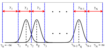
Figure 2: PAM system with input $X\in\mathcal{X}=\{x_{1},x_{2},\ldots,x_{q}\},x_{1}<x_{2}<\cdots<x_{q}$. $X$ is transmitted over an AWGN channel with noise variance $\sigma^{2}$ and mean 0. The channel is converted into a DMC by uniformly quantizing the continuous channel output $\widetilde{Y}$ to $N$ levels $\mathcal{Y}=\{y_{1},y_{2},\ldots,y_{N}\}$ based on $N+1$ thresholds $\Gamma=\{\gamma_{0},\gamma_{1},\ldots,\gamma_{N}\}$ with $\gamma_{1}=x_{1}-3\sigma$, $\gamma_{N-1}=x_{q}+3\sigma$, and $\gamma_{1}-\gamma_{2}=\gamma_{2}-\gamma_{3}=\cdots=\gamma_{N-2}-\gamma_{N-1}$.

We first convert the channel into a DMC, as shown in Fig. 2, with output $Y\in\mathcal{Y}=\{y_{1},y_{2},\ldots,y_{N}\}$, where $N\gg M$. More specifically, we create $N+1$ candidate thresholds $\Gamma=\{\gamma_{0},\gamma_{1},\ldots,\gamma_{N}\},\gamma_{0}=-\infty<\gamma_{1}<\cdots<\gamma_{N-1}<\gamma_{N}=+\infty$, such that the transition probability of the DMC is given by

$$P_{Y|X}(y_{j}|x_{i})=\int_{\gamma_{j-1}}^{\gamma_{j}}f_{\widetilde{Y}|X}(\widetilde{y}|x_{i})\mathrm{d}\widetilde{y}$$

for $i\in[q]$ and $j\in[N]$. In general, we can set $\gamma_{1}=x_{1}-3\sigma$ and $\gamma_{N-1}=x_{q}+3\sigma$, and set $\gamma_{j}=\gamma_{j-1}+(\gamma_{N-1}-\gamma_{1})/(N-2)$ for $j=2,\ldots,N-2$ to uniformly partition $[\gamma_{1},\gamma_{N-1}]$ into $N-2$ segments.

We can then use Algorithm 1 to find the optimal thresholds $\Theta$ from the candidate thresholds $\Gamma$ according to Proposition 1. In particular, if $\alpha$-MI-maximizing SDQs are of interest, the two low-complexity techniques discussed in Section IV are applicable here, according to Theorem 4 and the following lemma. We remark that Lemma 5 only requires $x_{1}<x_{2}<\cdots<x_{q}$ and $\gamma_{0}=-\infty<\gamma_{1}<\cdots<\gamma_{N-1}<\gamma_{N}=+\infty$. However, it does not depend on $P_{X}$ and the specific values of $\{x_{1},\ldots,x_{q},\gamma_{1},\ldots,\gamma_{N-1}\}$. Moreover, Lemma 5 also implies that if only $x_{1}<x_{2}<\cdots<x_{q}$ does not hold, $\{x_{1},\ldots,x_{q}\}$ can be relabelled to make $P_{Y|X}$ satisfy (8) such that Theorem 4 is also applicable.

Lemma 5

For the converted DMC shown in Fig. 2, $P_{Y|X}$ satisfies (8).

Proof:

For $1\leq i<q$ and $1\leq j\leq N$, we have

$$P_{Y|X}(y_{j}|x_{i})/P_{Y|X}(y_{j}|x_{i+1})$$

$$= \frac{\int_{\gamma_{j-1}}^{\gamma_{j}}f_{\widetilde{Y}|X}(\widetilde{y}|x_{i})\mathrm{d}\widetilde{y}}{\int_{\gamma_{j-1}}^{\gamma_{j}}f_{\widetilde{Y}|X}(\widetilde{y}|x_{i+1})\mathrm{d}\widetilde{y}}$$

$$= \frac{\int_{\gamma_{j-1}}^{\gamma_{j}}{f_{\widetilde{Y}|X}(\widetilde{y}|x_{i})}\big{/}{f_{\widetilde{Y}|X}(\widetilde{y}|x_{i+1})}f_{\widetilde{Y}|X}(\widetilde{y}|x_{i+1})\mathrm{d}\widetilde{y}}{\int_{\gamma_{j-1}}^{\gamma_{j}}f_{\widetilde{Y}|X}(\widetilde{y}|x_{i+1})\mathrm{d}\widetilde{y}}.$$ (17)

Since

$$\frac{f_{\widetilde{Y}|X}(\widetilde{y}|x_{i})}{f_{\widetilde{Y}|X}(\widetilde{y}|x_{i+1})}=\exp\left(\frac{(x_{i}-x_{i+1})(2\widetilde{y}-x_{i}-x_{i+1})}{2\sigma^{2}}\right)$$

keeps strictly decreasing when $\widetilde{y}$ increases from $\gamma_{j-1}$ to $\gamma_{j}$, we have

$$\frac{f_{\widetilde{Y}|X}(\gamma_{j-1}|x_{i})}{f_{\widetilde{Y}|X}(\gamma_{j-1}|x_{i+1})}>\frac{f_{\widetilde{Y}|X}(\widetilde{y}|x_{i})}{f_{\widetilde{Y}|X}(\widetilde{y}|x_{i+1})}>\frac{f_{\widetilde{Y}|X}(\gamma_{j}|x_{i})}{f_{\widetilde{Y}|X}(\gamma_{j}|x_{i+1})}$$ (18)

for $\gamma_{j-1}<\widetilde{y}<\gamma_{j}$. Then, based on (VI) and (18), we have

$$\frac{f_{\widetilde{Y}|X}(\gamma_{j-1}|x_{i})}{f_{\widetilde{Y}|X}(\gamma_{j-1}|x_{i+1})}>\frac{P_{Y|X}(y_{j}|x_{i})}{P_{Y|X}(y_{j}|x_{i+1})}>\frac{f_{\widetilde{Y}|X}(\gamma_{j}|x_{i})}{f_{\widetilde{Y}|X}(\gamma_{j}|x_{i+1})},$$

indicating that $P_{Y|X}$ satisfies (8). ∎

Next, for the converted DMC shown in Fig. 2, we compare the quantization performance of the DP method with the prior art quantizer design algorithms proposed for the general $q$-ary input DMC, i.e., the greedy combining algorithm [11, 12] and the KL-means algorithm [13]. The MI-maximizing quantizers are of interest, and the MI gap $I_{g}=I(X;Y)-I(X;Z)$ is used as the comparison metric, which is the smaller the better. In the simulations, we use uniform distribution for $P_{X}$. We set $\sigma=1$, $x_{i}=2i-q-1$ for $i\in[q]$, and $N=128$. $\mathcal{Y}$ is quantized to $M$ levels, $M=2,3,\ldots,20$. When the KL-means algorithm is used, we randomly choose $M$ out of $N$ points as the initial means (see [13]) for $T_{i}=100$ times, and for each time the KL-means algorithm runs for $T_{r}=100$ iterations to obtain a DQ, and finally the best ($I_{g}$ is minimized) DQ among the $T_{i}$ times is chosen. The simulation results are illustrated by Fig. 3. It is shown that the DP method performs better than both the greedy combining and KL-means algorithms, for different values of $q$.

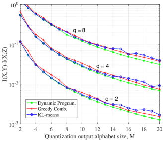
Figure 3: Performance of the DP method, the greedy combining [11, 12], and the KL-means [13] algorithms.

Moreover, note that the two low-complexity techniques are applicable here. The DP method has complexity $O(q(N-M)M)$ if applying the SMAWK algorithm and $O(q(N^{2}-M^{2}))$ if applying (13). In contrast, the greedy combining and KL-means algorithms have complexities $O(qN^{2}(N-M))$ and $O(T_{i}T_{r}qNM)$, respectively, and hence are much more complex than the DP method. As an example, we show the actual running time for these algorithms in Table I.

TABLE I: Average Running Time on a Standard Desktop for Different Quantizer Design Algorithms, Where A1–A5 Refer to the Original DP Algorithm Given by Algorithm 1, the DP Algorithm Optimized by Using the SMAWK Algorithm, the DP Algorithm Optimized by Using (13), the Greedy Combining Algorithm, and the KL-Means Algorithm, Respectively, and $q=2,M=8,T_{i}=100,T_{r}=100$ Are Used

Algorithm	Complexity	Running time in second
		$N=128$	$N=1000$
A1	$O(q(N-M)^{2}M)$	0.042	2.323
A2	$O(q(N-M)M)$	0.004	0.045
A3	$O(q(N^{2}-M^{2}))$	0.007	0.349
A4	$O(qN^{2}(N-M))$	0.206	89.496
A5	$O(T_{i}T_{r}qNM)$	1.353	10.063

Our final remark is that the optimal SDQ for the converted DMC shown by Fig. 2 may not be a globally optimal DQ. One toy counter-example has the following parameters: $(q,N,M,\sigma^{2})=(4,7,4,0.1)$, $(x_{1},x_{2},x_{3},x_{4})=(-3,-1,1,3)$, and $P_{X}=(0.53,0.23,0.23,0.01)$. We also find a counter-example among millions of test cases with uniformly distributed $P_{X}$ and randomly generated $P_{Y|X}$ which satisfies (8). Both counter-examples imply that the condition of (8) cannot solely guarantee the global optimality of an optimal SDQ among all DQs. To guarantee the global optimality, one sufficient condition given by Theorem 2 is to additionally require $\delta_{1},\delta_{2},\ldots,\delta_{N}$ to be located on a line. An intriguing but very hard problem is to find a more general sufficient condition.

VII Conclusion

In this paper, under the general cost function $C$ given by (3), we have presented a DP method with complexity $O(q(N-M)^{2}M)$ to obtain an optimal SDQ for $q$-ary input DMC. Two efficient techniques have been applied to reduce the DP method’s complexity once $w(\cdot,\cdot)$ satisfies the QI. One technique makes use of the SMAWK algorithm and achieves complexity $O(q(N-M)M)$. The other one is much easier to be implemented and achieves complexity $O(q(N^{2}-M^{2}))$. We have proved that when $\delta_{1},\delta_{2},\ldots,\delta_{N}$ defined by (4) are sequentially located on a line, the optimal SDQ is an optimal DQ and the two efficient techniques are applicable. This result generalizes the results of [3, 4, 5]. Next, we have showed that the cost function of an $\alpha$-MI-maximizing quantizer can be defined as a specific case of $C$. We have further proved that if the elements in $\mathcal{X}$ can be relabelled to make $P_{Y|X}$ satisfy (8), but not requiring $\delta_{1},\delta_{2},\ldots,\delta_{N}$ to be sequentially located on a line, the aforementioned two efficient techniques are applicable to the design of $\alpha$-MI-maximizing quantizer. Finally, we have demonstrated the application of our design method to the DMCs derived from AWGN channels with PAMs.

Appendix A Proof of Lemma 1

Note that for any quantizer $Q:\mathcal{Y}\to\mathcal{Z}$, $Q$ is specified by $P_{Z|Y}$, and $C(Q)$ given by (3) is a function of $P_{Z|Y}$. We now show $C(Q)$ is concave on $P_{Z|Y}$. For any $t\in[0,1]$ and any two quantizers $Q^{(1)},Q^{(2)}$ specified by $P^{(1)}_{Z|Y},P^{(2)}_{Z|Y}$, respectively, denote $Q$ as the quantizer specified by $P_{Z|Y}=tP^{(1)}_{Z|Y}+(1-t)P^{(2)}_{Z|Y}$, where the addition is element-wise. Then, for $x\in\mathcal{X}$ and $z\in\mathcal{Z}$, we have

$$P_{Z}(z) =tP^{(1)}_{Z}(z)+(1-t)P^{(2)}_{Z}(z),$$

$$P_{X|Z}(x|z) =\frac{tP^{(1)}_{Z}(z)}{P_{Z}(z)}P^{(1)}_{X|Z}(x|z)+$$

$$\quad\quad\quad\quad\quad\quad\frac{(1-t)P^{(2)}_{Z}(z)}{P_{Z}(z)}P^{(2)}_{X|Z}(x|z).$$

Since $\phi$ is concave on $P_{X|Z}$, we have

$$C(Q) =\sum_{z\in\mathcal{Z}}P_{Z}(z)\phi(P_{X|Z}(\cdot|z))$$

$$\geq\sum_{z\in\mathcal{Z}}\big{(}tP^{(1)}_{Z}(z)\phi(P^{(1)}_{X|Z}(\cdot|z))+$$

$$\quad\quad\quad\quad\quad\quad(1-t)P^{(2)}_{Z}(z)\phi(P^{(2)}_{X|Z}(\cdot|z))\big{)}$$

$$=tC(Q^{(1)})+(1-t)C(Q^{(2)}),$$

indicating that $C(Q)$ is concave on $P_{Z|Y}$. It is well known that there exists at least one extreme point, which corresponds to a DQ in this case, to make the concave function $C(Q)$ achieve its minima. This completes the proof.

Appendix B Proof of Theorem 2

1) $\to$ 2): If $\delta_{1},\delta_{2},\ldots,\delta_{N}$ are sequentially located on a line, they are definitely located on the line and both (6) and (7) hold. We relabel the elements in $\mathcal{X}$ to satisfy

$$P_{X|Y}(x_{i}|y_{1})d_{i+1}\geq P_{X|Y}(x_{i+1}|y_{1})d_{i},\forall i\in[q-1],$$ (19)

which is always possible. For any $1\leq i<i^{\prime}\leq q$, if $P_{X|Y}(x_{i^{\prime}}|y_{1})=0$, we have $d_{i^{\prime}}>0$ and

$$P_{X|Y}(x_{i}|y_{1})d_{i^{\prime}}\geq P_{X|Y}(x_{i^{\prime}}|y_{1})d_{i}.$$ (20)

If $P_{X|Y}(x_{i^{\prime}}|y_{1})>0$, we have $P_{X|Y}(x_{i^{\prime}-1}|y_{1})>0$ due to (19). Recursively, we have $P_{X|Y}(x_{k}|y_{1})>0$ for $i\leq k\leq i^{\prime}$. In this case, according to (19), we have

$$\frac{d_{i}}{P_{X|Y}(x_{i}|y_{1})}\leq\frac{d_{i+1}}{P_{X|Y}(x_{i+1}|y_{1})}\leq\cdots\leq\frac{d_{i^{\prime}}}{P_{X|Y}(x_{i^{\prime}}|y_{1})},$$

indicating that (20) also holds. Then, for $1\leq i<i^{\prime}\leq q$ and $1\leq j<j^{\prime}\leq N$, we have

$${P_{Y|X}(y_{j}|x_{i})}{P_{Y|X}(y_{j^{\prime}}|x_{i^{\prime}})}-{P_{Y|X}(y_{j^{\prime}}|x_{i})}{P_{Y|X}(y_{j}|x_{i^{\prime}})}$$

$$={(P_{X|Y}(x_{i}|y_{1})d_{i^{\prime}}-P_{X|Y}(x_{i^{\prime}}|y_{1})d_{i})(t_{j^{\prime}}-t_{j})}\cdot$$

$$\quad\quad\quad\quad\quad\quad\quad\quad P_{Y}(y_{j})P_{Y}(y_{j^{\prime}})/P_{X}(x_{i})/P_{X}(x_{i^{\prime}})$$

$$\geq 0,$$

indicating that the second statement of Theorem 2 is true.

2) $\to$ 3): This is a trivial conclusion.

3) $\to$ 1): Suppose that $\delta_{1},\delta_{2},\ldots,\delta_{N}$ are located on a line. As a result, (6) holds. Further assume that the elements in $\mathcal{X}$ can be relabelled to make $P_{Y|X}$ satisfy (3), and we implement the relabelling in this way. After that, for any $i\in[q-1]$ and $j\in[N-1]$, we have

$$0\leq {P_{X|Y}(x_{i}|y_{j})}{P_{X|Y}(x_{i+1}|y_{j+1})}-$$

$$\quad\quad\quad\quad\quad\quad{P_{X|Y}(x_{i}|y_{j+1})}{P_{X|Y}(x_{i+1}|y_{j})}$$

$$= (P_{X|Y}(x_{i}|y_{1})d_{i+1}-P_{X|Y}(x_{i+1}|y_{1})d_{i})(t_{j+1}-t_{j}).$$

Then, for any $i\in[q-1]$, we have

$$0\leq \sum_{j\in[N-1]}\big{(}{P_{X|Y}(x_{i}|y_{j})}{P_{X|Y}(x_{i+1}|y_{j+1})}-$$

$$\quad\quad\quad\quad\quad\quad{P_{X|Y}(x_{i}|y_{j+1})}{P_{X|Y}(x_{i+1}|y_{j})}\big{)}$$

$$= P_{X|Y}(x_{i}|y_{1})d_{i+1}-P_{X|Y}(x_{i+1}|y_{1})d_{i}.$$

As a result, if $t_{j+1}<t_{j}$ for some $j\in[N-1]$, we must have

$$P_{X|Y}(x_{i}|y_{1})d_{i+1}=P_{X|Y}(x_{i+1}|y_{1})d_{i},\forall i\in[q-1].$$ (21)

We now prove (21) is not true. If (21) holds, we have $P_{X|Y}(x_{i}|y_{1})>0,\forall i\in[q]$; otherwise, $P_{X|Y}(x_{i}|y_{1})=0,\forall i\in[q]$ can be derived but this is not true. Then, we have

$$\frac{d_{1}}{P_{X|Y}(x_{1}|y_{1})}=\frac{d_{2}}{P_{X|Y}(x_{2}|y_{1})}=\cdots=\frac{d_{q}}{P_{X|Y}(x_{q}|y_{1})}.$$

Further since $0=\sum_{i\in[q]}P_{X|Y}(x_{i}|y_{N})-1=\sum_{i\in[q]}(P_{X|Y}(x_{i}|y_{1})+t_{N}d_{i})-1=\sum_{i\in[q]}d_{i}$, we must have $d_{1}=d_{2}=\cdots=d_{q}=0$. In this case, we have $0=\mathbf{d}=\delta_{N}-\delta_{1}$, contradicting to the assumption that $\delta_{1}\neq\delta_{N}$. Therefore, (21) is not true and hence we have $t_{j+1}\geq t_{j},\forall j\in[N-1]$, indicating that $\delta_{1},\delta_{2},\ldots,\delta_{N}$ are sequentially located on the line.

Optimality: Suppose that $\delta_{1},\delta_{2},\ldots,\delta_{N}$ are sequentially located on a line. According to Lemma 2, there exists an optimal DQ $\tilde{Q}^{*}:\Delta\to\mathcal{Z}$ such that for any $z,z^{\prime}\in\mathcal{Z}$ with $z\neq z^{\prime}$, there exists a point that separates $\tilde{Q}^{*-1}(z)$ and $\tilde{Q}^{*-1}(z^{\prime})$ on the line. In this case, the equivalent quantizer of $\tilde{Q}^{*}$, $Q^{*}:\mathcal{Y}\to\mathcal{Z}$, is an optimal DQ as well as an optimal SDQ.

Appendix C Proof of Lemma 4

For $2\leq m\leq n<N$, let $t=\mathsf{sol}(n,m)$ for brevity. For any $m-1\leq k<t$, we have

$$\mathsf{dp}_{t}(n+1,m)-\mathsf{dp}_{k}(n+1,m)$$

$$= \mathsf{dp}_{t}(n,m)-w(t+1,n)+w(t+1,n+1)-$$

$$\quad\quad(\mathsf{dp}_{k}(n,m)-w(k+1,n)+w(k+1,n+1))$$

$$\leq w(t+1,n+1)+w(k+1,n)-$$

$$\quad\quad w(t+1,n)-w(k+1,n+1)$$

$$\leq 0,$$

where the last inequality holds because $w(\cdot,\cdot)$ satisfies the QI. Therefore, we have $\mathsf{sol}(n,m)=t\leq\mathsf{sol}(n+1,m)$.

We now continue to prove $\mathsf{sol}(n,m)\geq\mathsf{sol}(n,m-1)$. For $m=2$, we have $\mathsf{sol}(n,m)\geq\mathsf{sol}(n,m-1)=0$ trivially. For $m\geq 3$, let $t=\mathsf{sol}(n,m-1)$ for brevity. For any $m-1\leq k<t$, we have

$$\mathsf{dp}_{t}(n,m)-\mathsf{dp}_{k}(n,m)$$

$$= \mathsf{dp}(t,m-1)+\mathsf{dp}_{t}(n,m-1)-\mathsf{dp}(t,m-2)-$$

$$\quad\quad(\mathsf{dp}(k,m-1)+\mathsf{dp}_{k}(n,m-1)-\mathsf{dp}(k,m-2))$$

$$\leq \mathsf{dp}(k,m-2)+\mathsf{dp}(t,m-1)-$$

$$\quad\quad\mathsf{dp}(k,m-1)-\mathsf{dp}(t,m-2).$$

We continue the proof by first proving the following lemma.

Lemma 6

For $2\leq m\leq i<j\leq N$, denoting $\mathsf{dp}(i,m-1)+\mathsf{dp}(j,m)-\mathsf{dp}(i,m)-\mathsf{dp}(j,m-1)$ by $\psi(i,j,m)$, we have

$$\psi(i,j,m)\leq 0.$$

Proof:

Let $t=\mathsf{sol}(i,2)$ for brevity. We have

$$\psi(i,j,2) \leq\mathsf{dp}(i,1)+\mathsf{dp}_{t}(j,2)-\mathsf{dp}_{t}(i,2)-\mathsf{dp}(j,1)$$

$$=w(1,i)+w(t+1,j)-w(t+1,i)-w(1,j)$$

$$\leq 0.$$

We then inductively prove $\psi(i,j,m)\leq 0$ for $m\geq 3$ given $\psi(i,j,m-1)\leq 0$ for $m-1\leq i<j$.

Let $a=\mathsf{sol}(i,m)$ and $b=\mathsf{sol}(j,m-1)$ for brevity. Note that $m-1\leq a<i$. If $a<b$, we have

$$\psi(i,j,m)$$

$$\leq \mathsf{dp}_{a}(i,m-1)+\mathsf{dp}_{b}(j,m)-\mathsf{dp}_{a}(i,m)-\mathsf{dp}_{b}(j,m-1)$$

$$= \mathsf{dp}(a,m-2)+\mathsf{dp}(b,m-1)-$$

$$\quad\quad\quad\quad\quad\quad\quad\quad\quad\quad\mathsf{dp}(a,m-1)-\mathsf{dp}(b,m-2)$$

$$= \psi(a,b,m-1)$$

$$\leq 0.$$

If $a\geq b$, we have

$$\psi(i,j,m)$$

$$\leq \mathsf{dp}_{b}(i,m-1)+\mathsf{dp}_{a}(j,m)-\mathsf{dp}_{a}(i,m)-\mathsf{dp}_{b}(j,m-1)$$

$$= w(b+1,i)+w(a+1,j)-w(a+1,i)-w(b+1,j)$$

$$\leq 0.$$

This completes the proof of Lemma 6. ∎

At this point, we have $\mathsf{dp}_{t}(n,m)-\mathsf{dp}_{k}(n,m)\leq\psi(k,t,m-1)\leq 0$, implying $\mathsf{sol}(n,m)\geq\mathsf{sol}(n,m-1)$.

Appendix D Proof of Theorem 3

Lemma 7

Let $n$ be a positive integer. $A,B,C,D\in\mathbb{R}^{n}$ are located on a line with $A$ and $D$ being the endpoints. $\eta$ is a function which is concave on this line. If there exist $\gamma,\beta\in[0,1]$ such that $\gamma A+(1-\gamma)D=\beta B+(1-\beta)C$, we then have

$$\gamma\eta(A)+(1-\gamma)\eta(D)\leq\beta\eta(B)+(1-\beta)\eta(C).$$

Proof:

If $A=D$, Lemma 7 holds. For $A\neq D$, there exist unique $\theta,\tau\in[0,1]$ such that

$$B =\theta A+(1-\theta)D,$$

$$C =\tau A+(1-\tau)D.$$

Then, we have

$$\gamma A+(1-\gamma)D$$

$$= \beta B+(1-\beta)C$$

$$= (\beta\theta+(1-\beta)\tau)A+(\beta(1-\theta)+(1-\beta)(1-\tau))D,$$

which leads to

$$\gamma =\beta\theta+(1-\beta)\tau.$$

As a result, we have

$$\beta\eta(B)+(1-\beta)\eta(C)$$

$$\geq \beta(\theta\eta(A)+(1-\theta)\eta(D))+$$

$$\quad\quad\quad\quad\quad\quad(1-\beta)(\tau\eta(A)+(1-\tau)\eta(D))$$

$$= \gamma\eta(A)+(1-\gamma)\eta(D),$$

indicating that Lemma 7 is correct. ∎

Lemma 7 is indeed a well-known result for concave function. We now use it to simplify the proof of Theorem 3. For $1\leq r\leq s\leq N$, denote

$$a(r,s) =\sum_{j=r}^{s}P_{Y}(y_{j}),$$

$$b(r,s) =\sum_{j=r}^{s}\frac{P_{Y}(y_{j})}{a(r,s)}\delta_{j}.$$

Then, according to (5), we have

$$w(r,s)=a(r,s)\phi(b(r,s)).$$ (22)

Suppose $\delta_{1},\delta_{2},\ldots,\delta_{N}$ are sequentially located on a line. In such a case, for any $1\leq r<r^{\prime}\leq s<s^{\prime}\leq N$, $b(r,s),b(r,s^{\prime}),b(r^{\prime},s),b(r^{\prime},s^{\prime})$ are located on the line with $b(r,s)$ and $b(r^{\prime},s^{\prime})$ being the endpoints, and $\phi$ is concave on the line. Let $\gamma=a(r,s)/(a(r,s)+a(r^{\prime},s^{\prime}))$ and $\beta=a(r,s^{\prime})/(a(r,s^{\prime})+a(r^{\prime},s))$. We have $\gamma,\beta\in[0,1]$ and $\gamma b(r,s)+(1-\gamma)b(r^{\prime},s^{\prime})=\beta b(r,s^{\prime})+(1-\beta)b(r^{\prime},s)$. By applying (22) and Lemma 7, we have

$$(w(r,s)+w(r^{\prime},s^{\prime}))/(a(r,s)+a(r^{\prime},s^{\prime}))$$

$$= \gamma\phi(b(r,s))+(1-\gamma)\phi(r^{\prime},s^{\prime})$$

$$\leq \beta\phi(b(r,s^{\prime}))+(1-\beta)\phi(b(r^{\prime},s))$$

$$= (w(r,s^{\prime})+w(r^{\prime},s))/(a(r,s^{\prime})+a(r^{\prime},s)),$$

leading to $w(r,s)+w(r^{\prime},s^{\prime})\leq w(r,s^{\prime})+w(r^{\prime},s)$. This completes the proof.

Appendix E Proof of Theorem 4

Our goal is to prove

$$w_{\alpha}(r,s)+w_{\alpha}(r^{\prime},s^{\prime})-w_{\alpha}(r,s^{\prime})-w_{\alpha}(r^{\prime},s)\leq 0$$ (23)

for $\alpha\in(0,\infty]$ and for all $1\leq r<r^{\prime}\leq s<s^{\prime}\leq N$ given that the elements in $\mathcal{X}$ can be relabelled to make $P_{Y|X}$ satisfy (8). Since $w_{\alpha}(\cdot,\cdot)$ is independent from the labelling of the elements of $\mathcal{X}$, for convenience, we assume that the elements in $\mathcal{X}$ has been relabelled to make $P_{Y|X}$ satisfy (8).

For any $\mathbf{a}=(a_{i})_{1\leq i\leq q},\mathbf{b}=(b_{i})_{1\leq i\leq q}\in\mathbb{R}_{+}^{q}$, we use the following notations:

1. $\|\mathbf{a}\|_{1}=\sum_{i=1}^{q}a_{i}$,

2. $I_{min}(\mathbf{a})=\arg\min_{i}(a_{i}=0)$,

3. $I_{max}(\mathbf{a})=\arg\max_{i}(a_{i}=0)$,

4. $\mathbf{a}+\mathbf{b}=(a_{i}+b_{i})_{1\leq i\leq q}$,

The proof is divided into four parts based on the four cases of $\alpha=1$, $\alpha\in(0,1)$, $\alpha\in(1,\infty)$, and $\alpha=\infty$.

Part I: $\alpha=1$

Denote $\mathbf{p},\mathbf{a},\mathbf{b},\mathbf{c}\in\mathbb{R}_{+}^{q}$, with $p_{i},a_{i},b_{i},c_{i}$ given by

$$p_{i} =P_{X}(x_{i}),$$

$$a_{i} =\sum_{j=r}^{r^{\prime}-1}p_{i}P_{Y|X}(y_{j}|x_{i}),$$

$$b_{i} =\sum_{j=r^{\prime}}^{s}p_{i}P_{Y|X}(y_{j}|x_{i}),$$

$$c_{i} =\sum_{j=s+1}^{s^{\prime}}p_{i}P_{Y|X}(y_{j}|x_{i}).$$ (24)

Given (8), we have

$$\mathbf{a}\succeq\mathbf{b},\mathbf{b}\succeq\mathbf{c},\mathbf{a}\succeq\mathbf{c},$$ (25)

where $\succeq$ is defined in (2). From (8) and (25), we can easily derive

$$\left\{\begin{array}[]{l}I_{min}(\mathbf{a})\leq I_{min}(\mathbf{b})\leq I_{max}(\mathbf{a})\leq I_{max}(\mathbf{b}),\\ I_{min}(\mathbf{b})\leq I_{min}(\mathbf{c})\leq I_{max}(\mathbf{b})\leq I_{max}(\mathbf{c}),\\ u_{i}>0,\forall\mathbf{u}\in\{\mathbf{a},\mathbf{b},\mathbf{c}\},i\in[I_{min}(\mathbf{u}),I_{max}(\mathbf{u})].\end{array}\right.$$ (26)

For any $\mathbf{u}\in\mathbb{R}_{+}^{q}$, define

$$g(\mathbf{u})=\sum_{i=1}^{q}u_{i}\log\frac{\|\mathbf{u}\|_{1}}{u_{i}},$$

where we let $u_{i}\log\frac{\|\mathbf{u}\|_{1}}{u_{i}}=0$ if $u_{i}=0$. Here the natural logarithm in base $e$ is used. For other bases, the following proof can be similarly carried out. In addition, let

$$f(\mathbf{a},\mathbf{b},\mathbf{c}) =g(\mathbf{a}+\mathbf{b})+g(\mathbf{b}+\mathbf{c})-g(\mathbf{a}+\mathbf{b}+\mathbf{c})-g(\mathbf{b})$$

$$=w_{\alpha}(r,s)+w_{\alpha}(r^{\prime},s^{\prime})-w_{\alpha}(r,s^{\prime})-w_{\alpha}(r^{\prime},s).$$

To prove $f(\mathbf{a},\mathbf{b},\mathbf{c})\leq 0$, our idea is to properly modify $\mathbf{a},\mathbf{b}$, and $\mathbf{c}$ in a series of steps, where after each step, $f(\mathbf{a},\mathbf{b},\mathbf{c})$ keeps nondecreasing and finally becomes zero. We summarize the procedure in Algorithm 3, following which we also provide the remarks.

Algorithm 3 A series of modifications on $\mathbf{a},\mathbf{b}$, and $\mathbf{c}$ such that $f(\mathbf{a},\mathbf{b},\mathbf{c})$ keeps nondecreasing and finally becomes zero

0:  $\mathbf{a},\mathbf{b},\mathbf{c}$ given by (E).

1:  $k\leftarrow 1$.

2:  while $k<q$ and $\mathbf{a}\neq\mathbf{0}$ do

3:     if $a_{k}b_{k+1}>a_{k+1}b_{k}$ then

4:        $a_{i}\leftarrow a_{k+1}b_{i}/b_{k+1},\forall i\in[k]$.

5:     end if

6:     if $b_{k}c_{k+1}>b_{k+1}c_{k}$ then

7:        if $b_{k+1}>0$ then

8:           $c_{i}\leftarrow b_{i}c_{k+1}/b_{k+1},\forall i\in[k]$.

9:        else

10:           $c_{i}\leftarrow 0,\forall i=k+1,k+2,\ldots,q$.

11:        end if

12:     end if

13:     $k\leftarrow k+1$.

14:  end while

15:  $//$ At this point, we have $f(\mathbf{a},\mathbf{b},\mathbf{c})=0$.

Remark 1

Note that for $k=1$, (25), (26), and the following conditions hold:

$$a_{i}b_{j}=a_{j}b_{i},b_{i}c_{j}=b_{j}c_{i},a_{i}c_{j}=a_{j}c_{i},\forall 1\leq i<j\leq k.$$ (27)

Inductively, suppose these conditions ((25)–(27)) hold for $k<q$. In the subsequent remarks, we will prove that these conditions can keep $f(\mathbf{a},\mathbf{b},\mathbf{c})$ nondecreasing after any modification of those in lines 4, 8, 10 made to $\mathbf{a},\mathbf{b},\mathbf{c}$. We will also prove that when Algorithm 3 reaches line 13 and increases $k$ by 1, either $\mathbf{a}=0$ or these conditions will still hold. It can be easily verified that either $\mathbf{a}=0$ or these conditions that hold for $k=q$ can lead to $f(\mathbf{a},\mathbf{b},\mathbf{c})=0$ at line 15.

Remark 2 (for line 4)

Throughout this remark, let $k,\mathbf{a},\mathbf{b},\mathbf{c}$ refer to those at the beginning of line 4 (before the modification). Let $\mathbf{a}^{\prime}$ refer to the $\mathbf{a}$ at the end of line 4 (after the modification). Our goal is to prove

$$f(\mathbf{a},\mathbf{b},\mathbf{c})\leq f(\mathbf{a}^{\prime},\mathbf{b},\mathbf{c}),$$ (28)

i.e., to prove $f(\mathbf{a},\mathbf{b},\mathbf{c})$ keeps nondecreasing after the modification in line 4.

Let $T=a_{k+1}b_{k}/(a_{k}b_{k+1})$. For any $i\in[k]$, according to (27), we have $Ta_{i}b_{k}=Ta_{k}b_{i}=a^{\prime}_{i}b_{k}$. This leads to $Ta_{i}=a^{\prime}_{i}$; otherwise, we can easily derive a contradiction for $Ta_{i}\neq a^{\prime}_{i}$. Let $t\in[T,1]$ be a variable. Denote $\mathbf{a}{(t)}=\left(a_{i}{(t)}\right)_{1\leq i\leq q}$ with

$$a_{i}{(t)}=\begin{cases}a_{i}t,&i\in[k],\\ a_{i},&i\notin[k].\end{cases}$$

Then, we have $\mathbf{a}(1)=\mathbf{a}$ and $\mathbf{a}(T)=\mathbf{a}^{\prime}$.

We are now to prove

$$\mathbf{a}(t)\succeq\mathbf{b},\mathbf{a}(t)\succeq\mathbf{c},\forall t\in[T,1].$$ (29)

For any $1\leq i<j\leq k$ or $k<i<j\leq q$, we can easily verify $a_{i}(t)b_{j}\geq a_{j}(t)b_{i}$ according to (25). For $1\leq i\leq k<j\leq q$, if $a_{j}(t)b_{i}=0$, we also have $a_{i}(t)b_{j}\geq a_{j}(t)b_{i}$. If $a_{j}(t)b_{i}>0$, according to (25) and (26), we have $b_{l}>0,\forall l\in[i,j]$, leading to $a_{i}(t)/b_{i}\geq a_{k+1}/b_{k+1}\geq a_{j}/b_{j}$. Thus, $\mathbf{a}(t)\succeq\mathbf{b}$ holds. To prove $\mathbf{a}(t)\succeq\mathbf{c}$, similarly, we only need to prove $a_{i}(t)c_{j}\geq a_{j}(t)c_{i}$ for $1\leq i\leq k<j\leq q$ and $a_{j}(t)c_{i}>0$, for which we also have $b_{j},c_{j}>0$ according to (25) and (26). Additionally, since $\mathbf{a}(t)\succeq\mathbf{b}$ holds, we have $a_{i}(t)/a_{j}(t)\geq b_{i}/b_{j}\geq c_{i}/c_{j}$. This completes the proof of (29). Moreover, according to (27), we have

$$a_{i}(t)b_{j}=a_{j}(t)b_{i},~{} a_{i}(t)c_{j}=a_{j}(t)c_{i},$$

$$\forall t\in[T,1],1\leq i<j\leq k.$$ (30)

For $t\in(T,1)$, we have

$$\frac{\partial f(\mathbf{a}(t),\mathbf{b},\mathbf{c})}{\partial t}$$

$$= \sum_{i\in[k],a_{i}>0}a_{i}\left(\log\frac{\|\mathbf{a}(t)+\mathbf{b}\|_{1}}{a_{i}(t)+b_{i}}-\log\frac{\|\mathbf{a}(t)+\mathbf{b}+\mathbf{c}\|_{1}}{a_{i}(t)+b_{i}+c_{i}}\right)$$

$$\leq 0,$$ (31)

where the last inequality is due to $\frac{\|\mathbf{a}(t)+\mathbf{b}\|_{1}}{a_{i}(t)+b_{i}}\leq\frac{\|\mathbf{a}(t)+\mathbf{b}+\mathbf{c}\|_{1}}{a_{i}(t)+b_{i}+c_{i}}$ based on (25), (27), (29), and (2). Moreover, since $f(\mathbf{a}(t),\mathbf{b},\mathbf{c})$ is continuous at $t\in[T,1]$, we have $f(\mathbf{a},\mathbf{b},\mathbf{c})=f(\mathbf{a}(1),\mathbf{b},\mathbf{c})\leq f(\mathbf{a}(T),\mathbf{b},\mathbf{c})=f(\mathbf{a}^{\prime},\mathbf{b},\mathbf{c})$, leading to (28).

If $k=I_{max}(\mathbf{a})<I_{max}(\mathbf{b})$, we have $\mathbf{a}^{\prime}=\mathbf{0}$, in which case $f(\mathbf{a}^{\prime},\mathbf{b},\mathbf{c})=0$ holds and the proof of part I is completed. For $k<I_{max}(\mathbf{a})$ or $I_{max}(\mathbf{a})=I_{max}(\mathbf{b})$, we always have $\mathbf{a^{\prime}}\neq\mathbf{0}$. After replacing $\mathbf{a}$ by $\mathbf{a}^{\prime}$, (25)–(27) still hold according to (29) and (2), except that $I_{min}(\mathbf{a})$ and $I_{max}(\mathbf{a})$ in (26) are undefined for the case of $\mathbf{a}=\mathbf{0}$. However, this exception does not affect the correctness of the proof of Part I.

Remark 3 (for line 8)

Throughout this remark, let $k,\mathbf{a},\mathbf{b},\mathbf{c}$ refer to those at the beginning of line 8. Let $\mathbf{c}^{\prime}$ refer to the $\mathbf{c}$ at the end of line 8. Our goal is to prove

$$f(\mathbf{a},\mathbf{b},\mathbf{c})\leq f(\mathbf{a},\mathbf{b},\mathbf{c}^{\prime}).$$ (32)

Let $T=b_{k+1}c_{k}/(b_{k}c_{k+1})$. For any $i\in[k]$, according to (27), we have $c_{i}b_{k}=c_{k}b_{i}=Tc^{\prime}_{i}b_{k}$. This leads to $c_{i}=Tc^{\prime}_{i}$ due to $b_{k}>0$. Let $t\in[T,1]$ be a variable. Denote $\mathbf{c}^{\prime}{(t)}=\left(c^{\prime}_{i}{(t)}\right)_{1\leq i\leq q}$ with

$$c^{\prime}_{i}{(t)}=\begin{cases}c^{\prime}_{i}t,&i\in[k],\\ c^{\prime}_{i},&i\notin[k].\end{cases}$$

Then, we have $\mathbf{c}^{\prime}(1)=\mathbf{c}^{\prime}$ and $\mathbf{c}^{\prime}(T)=\mathbf{c}$.

Similar to (29), we have

$$\mathbf{b}\succeq\mathbf{c}^{\prime}(t),\mathbf{a}\succeq\mathbf{c}^{\prime}(t),\forall t\in[T,1].$$ (33)

Meanwhile, similar to (2), we have

$$a_{i}c^{\prime}_{j}(t)=a_{j}c^{\prime}_{i}(t),~{} b_{i}c^{\prime}_{j}(t)=b_{j}c^{\prime}_{i}(t),$$

$$\forall t\in[T,1],1\leq i<j\leq k.$$ (34)

Then, for $t\in(T,1)$, we have

$$\frac{\partial f(\mathbf{a},\mathbf{b},\mathbf{c}^{\prime}(t))}{\partial t}$$

$$= \sum_{i\in[k],c^{\prime}_{i}>0}c^{\prime}_{i}\left(\log\frac{\|\mathbf{b}+\mathbf{c}^{\prime}(t)\|_{1}}{b_{i}+c^{\prime}_{i}(t)}-\log\frac{\|\mathbf{a}+\mathbf{b}+\mathbf{c}^{\prime}(t)\|_{1}}{a_{i}+b_{i}+c^{\prime}_{i}(t)}\right)$$

$$\geq 0,$$ (35)

where the last inequality is due to $\frac{\|\mathbf{b}+\mathbf{c}^{\prime}(t)\|_{1}}{b_{i}+c^{\prime}_{i}(t)}\geq\frac{\|\mathbf{a}+\mathbf{b}+\mathbf{c}^{\prime}(t)\|_{1}}{a_{i}+b_{i}+c^{\prime}_{i}(t)}$ based on (25), (27), (33), and (3). Moreover, since $f(\mathbf{a},\mathbf{b},\mathbf{c}^{\prime}(t))$ is continuous at $t\in[T,1]$, we have $f(\mathbf{a},\mathbf{b},\mathbf{c})=f(\mathbf{a},\mathbf{b},\mathbf{c}^{\prime}(T))\leq f(\mathbf{a},\mathbf{b},\mathbf{c}^{\prime}(1))=f(\mathbf{a},\mathbf{b},\mathbf{c}^{\prime})$, leading to (32). In addition, after replacing $\mathbf{c}$ by $\mathbf{c}^{\prime}$, (25)–(27) still hold according to (33) and (3).

Remark 4 (for line 10)

Throughout this remark, let $k,\mathbf{a},\mathbf{b},\mathbf{c}$ refer to those at the beginning of line 10. Let $\mathbf{c}^{*}$ refer to the $\mathbf{c}$ at the end of line 10. Our goal is to prove

$$f(\mathbf{a},\mathbf{b},\mathbf{c})\leq f(\mathbf{a},\mathbf{b},\mathbf{c}^{*}),$$ (36)

Let $t\in[0,1]$ be a variable. Denote $\mathbf{c}{(t)}=\left(c_{i}{(t)}\right)_{1\leq i\leq q}$ with

$$c_{i}{(t)}=\begin{cases}c_{i},&i\in[k],\\ c_{i}t,&i\notin[k].\end{cases}$$

Then, we have $\mathbf{c}(0)=\mathbf{c}^{*}$ and $\mathbf{c}(1)=\mathbf{c}$. Note that if Algorithm 3 reaches line 10, we must have $k=I_{max}(\mathbf{b})$ according to (26). As a result, we have $a_{i}=b_{i}=0,\forall i=k+1,k+2,\ldots,q$. Then, for $t\in(0,1)$, we have

$$\frac{\partial f(\mathbf{a},\mathbf{b},\mathbf{c}(t))}{\partial t}$$

$$= \sum_{k<i\leq q,c_{i}>0}c_{i}\left(\log\frac{\|\mathbf{b}+\mathbf{c}(t)\|_{1}}{c_{i}(t)}-\log\frac{\|\mathbf{a}+\mathbf{b}+\mathbf{c}(t)\|_{1}}{c_{i}(t)}\right)$$

$$\leq 0.$$ (37)

Since $f(\mathbf{a},\mathbf{b},\mathbf{c}(t))$ is continuous at $t\in[0,1]$, we have $f(\mathbf{a},\mathbf{b},\mathbf{c})=f(\mathbf{a},\mathbf{b},\mathbf{c}(1))\leq f(\mathbf{a},\mathbf{b},\mathbf{c}(0))=f(\mathbf{a},\mathbf{b},\mathbf{c}^{*})$, leading to (36). In addition, after replacing $\mathbf{c}$ by $\mathbf{c}^{*}$, it can be easily verified that (25)–(27) still hold.

Remark 5 (for line 13)

Let $\mathbf{a},\mathbf{b},\mathbf{c}$ refer to those at the beginning of line 13. Let $v$ be the value of $k$ at the end of line 13. If $\mathbf{a}=\mathbf{0}$, the proof of this part is indeed completed. Suppose $\mathbf{a}\neq\mathbf{0}$. Our final task is to prove that (25)–(27) still hold for $k=v$, since these conditions will be used for $k=v$ for the proof of (28), (32), and (36).

In the previous remarks, we have proved that (25)–(27) hold for $k=v-1$, no matter the modifications in lines 4, 8, and 10 have been made or not. As a result, (25) and (26) still hold for $k=v$. In order to prove (27) for $k=v$, our task becomes to prove

$$a_{i}b_{v}=a_{v}b_{i},b_{i}c_{v}=b_{v}c_{i},a_{i}c_{v} =a_{v}c_{i},\forall i\in[v-1].$$ (38)

Note that when Algorithm 3 reaches line 13, we always have $a_{v-1}b_{v}=a_{v}b_{v-1}\text{~{}and~{}}b_{v-1}c_{v}=b_{v}c_{v-1}$. Based on this condition and that (27) holds for $k=v-1$, we can easily derive (38). At this point, the proof of Part I is completed.

Part II: $\alpha\in(0,1)$

Denote $\mathbf{p},\mathbf{a},\mathbf{b},\mathbf{c}\in\mathbb{R}_{+}^{q}$ by (E). For any $\mathbf{u}\in\mathbb{R}_{+}^{q}$, define

$$g(\mathbf{u})=\left(\sum_{i=1}^{q}p_{i}^{1-\alpha}u_{i}^{\alpha}\right)^{1/\alpha}.$$ (39)

In this case, we also have

$$f(\mathbf{a},\mathbf{b},\mathbf{c}) =g(\mathbf{a}+\mathbf{b})+g(\mathbf{b}+\mathbf{c})-g(\mathbf{a}+\mathbf{b}+\mathbf{c})-g(\mathbf{b})$$

$$=w_{\alpha}(r,s)+w_{\alpha}(r^{\prime},s^{\prime})-w_{\alpha}(r,s^{\prime})-w_{\alpha}(r^{\prime},s).$$

To prove $f(\mathbf{a},\mathbf{b},\mathbf{c})\leq 0$, our idea is the same as that in Part I. In this case, we indeed only need to prove (28), (32), and (36) under the new definition of $g:\mathbb{R}_{+}^{q}\to\mathbb{R}$ given by (39). To this end, our task becomes to prove $\frac{\partial f}{\partial t}\leq 0,\frac{\partial f}{\partial t}\geq 0$, and $\frac{\partial f}{\partial t}\leq 0$ as what we do in (2), (3), and (4), respectively. We complete these proofs below, where the notations correspond to those in (2), (3), and (4), except that $g$ is replaced by that defined by (39).

Proof of $\frac{\partial f}{\partial t}\leq 0$ corresponding to (2): We have

$$\frac{\partial f(\mathbf{a}(t),\mathbf{b},\mathbf{c})}{\partial t}$$

$$= \sum_{i\in[k],a_{i}>0}p_{i}^{1-\alpha}a_{i}\left(\left(\sum_{j=1}^{q}p_{j}^{1-\alpha}\left(\frac{a_{j}(t)+b_{j}}{a_{i}(t)+b_{i}}\right)^{\alpha}\right)^{\frac{1-\alpha}{\alpha}}-\right.$$

$$\quad\quad\quad\left.\left(\sum_{j=1}^{q}p_{j}^{1-\alpha}\left(\frac{a_{j}(t)+b_{j}+c_{j}}{a_{i}(t)+b_{i}+c_{i}}\right)^{\alpha}\right)^{\frac{1-\alpha}{\alpha}}\right)$$

$$\leq 0,$$

where the last inequality is due to $\frac{a_{j}(t)+b_{j}}{a_{i}(t)+b_{i}}\leq\frac{a_{j}(t)+b_{j}+c_{j}}{a_{i}(t)+b_{i}+c_{i}}$ based on (25), (27), (29), and (2).

Proof of $\frac{\partial f}{\partial t}\leq 0$ corresponding to (3): We have

$$\frac{\partial f(\mathbf{a},\mathbf{b},\mathbf{c}^{\prime}(t))}{\partial t}$$

$$= \sum_{i\in[k],c^{\prime}_{i}>0}p_{i}^{1-\alpha}c^{\prime}_{i}\left(\left(\sum_{j=1}^{q}p_{j}^{1-\alpha}\left(\frac{b_{j}+c^{\prime}_{j}(t)}{b_{i}+c^{\prime}_{i}(t)}\right)^{\alpha}\right)^{\frac{1-\alpha}{\alpha}}-\right.$$

$$\quad\quad\quad\left.\left(\sum_{j=1}^{q}p_{j}^{1-\alpha}\left(\frac{a_{j}+b_{j}+c^{\prime}_{j}(t)}{a_{i}+b_{i}+c^{\prime}_{i}(t)}\right)^{\alpha}\right)^{\frac{1-\alpha}{\alpha}}\right)$$

$$\geq 0,$$

where the last inequality is due to $\frac{b_{j}+c^{\prime}_{j}(t)}{b_{i}+c^{\prime}_{i}(t)}\geq\frac{a_{j}+b_{j}+c^{\prime}_{j}(t)}{a_{i}+b_{i}+c^{\prime}_{i}(t)}$ based on (25), (27), (33), and (3).

Proof of $\frac{\partial f}{\partial t}\leq 0$ corresponding to (4): We have

$$\frac{\partial f(\mathbf{a},\mathbf{b},\mathbf{c}(t))}{\partial t}$$

$$= \sum_{k<i\leq q,c_{i}>0}p_{i}^{1-\alpha}c_{i}\left(\left(\sum_{j=1}^{q}p_{j}^{1-\alpha}\left(\frac{b_{j}+c_{j}(t)}{c_{i}(t)}\right)^{\alpha}\right)^{\frac{1-\alpha}{\alpha}}-\right.$$

$$\quad\quad\quad\left.\left(\sum_{j=1}^{q}p_{j}^{1-\alpha}\left(\frac{a_{j}+b_{j}+c_{j}(t)}{c_{i}(t)}\right)^{\alpha}\right)^{\frac{1-\alpha}{\alpha}}\right)$$

$$\leq 0.$$

Part III: $\alpha\in(1,\infty)$

We omit the proof in this part since it can be carried out almost the same as that in Part II for $\alpha\in(0,1)$.

Part IV: $\alpha=\infty$

Set $\mathbf{a},\mathbf{b},\mathbf{c}$ with $a_{i},b_{i},c_{i}$ given by

$$a_{i} =\sum_{j=r}^{r^{\prime}-1}P_{Y|X}(y_{j}|x_{i}),$$

$$b_{i} =\sum_{j=r^{\prime}}^{s}P_{Y|X}(y_{j}|x_{i}),$$

$$c_{i} =\sum_{j=s+1}^{s^{\prime}}P_{Y|X}(y_{j}|x_{i}).$$

In this case, (25) still holds. Let $i=\arg\max_{1\leq t\leq q}(a_{t}+b_{t}),j=\arg\max_{1\leq t\leq q}(b_{t}+c_{t}),k=\arg\max_{1\leq t\leq q}(a_{t}+b_{t}+c_{t})$, and $l=\arg\max_{1\leq t\leq q}b_{t}$. Then, we have

$$w_{\alpha}(r,s)+w_{\alpha}(r^{\prime},s^{\prime})-w_{\alpha}(r,s^{\prime})-w_{\alpha}(r^{\prime},s)$$

$$= -(a_{i}+b_{i})-(b_{j}+c_{j})+(a_{k}+b_{k}+c_{k})+b_{l}$$

$$= -(a_{i}+b_{i})-(b_{j}+c_{j})+(a_{k}+b_{k})+$$

$$\,\,\,\quad\quad\quad\quad\quad\quad\quad\quad\quad\quad(b_{l}+c_{l})+(c_{k}-c_{l})$$

$$\leq c_{k}-c_{l}.$$

Based on a similar deduction, we indeed have $w_{\alpha}(r,s)+w_{\alpha}(r^{\prime},s^{\prime})-w_{\alpha}(r,s^{\prime})-w_{\alpha}(r^{\prime},s)\leq\min\{a_{k}-a_{l},b_{l}-b_{k},c_{k}-c_{l}\}$. If $\min\{a_{k}-a_{l},b_{l}-b_{k},c_{k}-c_{l}\}>0$, we have both $a_{k}b_{l}>a_{l}b_{k}$ and $b_{k}c_{l}<b_{l}c_{k}$, leading to a contradiction to (25). Therefore, we must have $\min\{a_{k}-a_{l},b_{l}-b_{k},c_{k}-c_{l}\}\leq 0$, implying (23) is true.

References

• [1] X. He, K. Cai, W. Song, and Z. Mei, “Dynamic programming for quantization of $q$-ary input discrete memoryless channels,” in Proc. IEEE Int. Symp. Inf. Theory, Jul. 2019, pp. 450–454.
• [2] T. H. Cormen, C. E. Leiserson, R. L. Rivest, and C. Stein, Introduction to Algorithms: 2nd Edition.   Cambridge, MA, USA: MIT Press, 2001.
• [3] B. M. Kurkoski and H. Yagi, “Quantization of binary-input discrete memoryless channels,” IEEE Trans. Inf. Theory, vol. 60, no. 8, pp. 4544–4552, Aug. 2014.
• [4] K. Iwata and S. Ozawa, “Quantizer design for outputs of binary-input discrete memoryless channels using SMAWK algorithm,” in Proc. IEEE Int. Symp. Inf. Theory, Jun. 2014, pp. 191–195.
• [5] Y. Sakai and K. Iwata, “Optimal quantization of B-DMCs maximizing $\alpha$-mutual information with monge property,” in Proc. IEEE Int. Symp. Inf. Theory, Jun. 2017, pp. 2668–2672.
• [6] A. Aggarwal, M. M. Klawe, S. Moran, P. Shor, and R. Wilber, “Geometric applications of a matrix-searching algorithm,” Algorithmica, vol. 2, no. 1, pp. 195–208, Nov. 1987.
• [7] B. Nazer, O. Ordentlich, and Y. Polyanskiy, “Information-distilling quantizers,” in Proc. IEEE Int. Symp. Inf. Theory, Jun. 2017, pp. 96–100.
• [8] E. Laber, M. Molinaro, and F. M. Pereira, “Binary partitions with approximate minimum impurity,” in Proc. 35th Int. Conf. Machine Learning, vol. 80, Stockholmsmässan, Stockholm Sweden, Jul. 2018, pp. 2854–2862.
• [9] D. Burshtein, V. Della Pietra, D. Kanevsky, and A. Nádas, “Minimum impurity partitions,” Ann. Statist., vol. 20, no. 3, pp. 1637–1646, Sep. 1992.
• [10] D. Coppersmith, S. J. Hong, and J. R. Hosking, “Partitioning nominal attributes in decision trees,” Data Mining and Knowledge Discovery, vol. 3, no. 2, pp. 197–217, Jun. 1999.
• [11] B. M. Kurkoski, K. Yamaguchi, and K. Kobayashi, “Noise thresholds for discrete LDPC decoding mappings,” in Proc. IEEE Global Commun. Conf., Dec. 2008, pp. 1–5.
• [12] Y. Sakai and K. Iwata, “Suboptimal quantizer design for outputs of discrete memoryless channels with a finite-input alphabet,” in Proc. IEEE Int. Symp. Inf. Theory and Its Applications, Nov. 2014, pp. 120–124.
• [13] J. A. Zhang and B. M. Kurkoski, “Low-complexity quantization of discrete memoryless channels,” in Proc. IEEE Int. Symp. Inf. Theory and Its Applications, Oct. 2016, pp. 448–452.
• [14] S. Hassanpour, D. Wuebben, and A. Dekorsy, “Overview and investigation of algorithms for the information bottleneck method,” in Proc. 11th Int. ITG Conf. on Systems, Commun. and Coding, Feb. 2017, pp. 1–6.
• [15] J. Lewandowsky, M. Stark, and G. Bauch, “Message alignment for discrete LDPC decoders with quadrature amplitude modulation,” in Proc. IEEE Int. Symp. Inf. Theory, Jun. 2017, pp. 2925–2929.
• [16] C. A. Aslam, Y. L. Guan, and K. Cai, “Read and write voltage signal optimization for multi-level-cell (MLC) NAND flash memory,” IEEE Trans. Commun., vol. 64, no. 4, pp. 1613–1623, Feb. 2016.
• [17] Z. Mei, K. Cai, L. Shi, and X. He, “On channel quantization for spin-torque transfer magnetic random access memory,” IEEE Trans. Commun., vol. 67, no. 11, pp. 7526–7539, Nov. 2019.
• [18] Z. Mei, K. Cai, and X. He, “Deep learning-aided dynamic read thresholds design for multi-level-cell flash memories,” IEEE Trans. Commun., vol. 68, no. 5, pp. 2850–2862, May 2020.
• [19] J. Wang, K. Vakilinia, T.-Y. Chen, T. Courtade, G. Dong, T. Zhang, H. Shankar, and R. Wesel, “Enhanced precision through multiple reads for LDPC decoding in flash memories,” IEEE J. Sel. Areas Commun., vol. 32, no. 5, pp. 880–891, May 2014.
• [20] X. He, K. Cai, and Z. Mei, “Mutual information-maximizing quantized belief propagation decoding of regular LDPC codes,” arXiv, 2019. [Online]. Available: https://arxiv.org/abs/1904.06666
• [21] X. He, K. Cai, and Z. Mei, “On finite alphabet iterative decoding of LDPC codes with high-order modulation,” IEEE Commun. Lett., vol. 23, no. 11, pp. 1913–1917, Nov. 2019.
• [22] F. F. Yao, “Efficient dynamic programming using quadrangle inequalities,” in Proc. 12th Annual ACM Symposium on Theory of Computing.   New York, NY, USA: ACM, 1980, pp. 429–435.
• [23] S. Verdú, “$\alpha$-mutual information,” in Proc. IEEE Information Theory and Applications Workshop, Feb. 2015, pp. 1–6.
• [24] S. Ho and S. Verdú, “Convexity/concavity of Rényi entropy and $\alpha$-mutual information,” in Proc. IEEE Int. Symp. Inf. Theory, Jun. 2015, pp. 745–749.
• [25] I. Csiszár, “Generalized cutoff rates and Rényi’s information measures,” IEEE Trans. Inf. Theory, vol. 41, no. 1, pp. 26–34, Jan. 1995.
• [26] W. Bein, M. J. Golin, L. L. Larmore, and Y. Zhang, “The Knuth-Yao quadrangle-inequality speedup is a consequence of total monotonicity,” ACM Trans. Algorithms, vol. 6, no. 1, pp. 17:1–17:22, Dec. 2009.
• [27] R. Gallager, “A simple derivation of the coding theorem and some applications,” IEEE Trans. Inf. Theory, vol. 11, no. 1, pp. 3–18, Jan. 1965.
• [28] Y. Polyanskiy and S. Verdú, “Arimoto channel coding converse and Rényi divergence,” in Proc. Annual Allerton Conference on Communication, Control, and Computing, Sep. 2010, pp. 1327–1333.