Optimal Closures in a Simple Model for Turbulent Flows

Abstract

In this work we introduce a computational framework for determining optimal closures of the eddy-viscosity type for Large-Eddy Simulations (LES) of a broad class of PDE models, such as the Navier-Stokes equation. This problem is cast in terms of PDE-constrained optimization where an error functional representing the misfit between the target and predicted observations is minimized with respect to the functional form of the eddy viscosity in the closure relation. Since this leads to a PDE optimization problem with a nonstandard structure, the solution is obtained computationally with a flexible and efficient gradient approach relying on a combination of modified adjoint-based analysis and Sobolev gradients. By formulating this problem in the continuous setting we are able to determine the optimal closure relations in a very general form subject only to some minimal assumptions. The proposed framework is thoroughly tested on a model problem involving the LES of the 1D Kuramoto-Sivashinsky equation, where optimal forms of the eddy viscosity are obtained as generalizations of the standard Smagorinsky model. It is demonstrated that while the solution trajectories corresponding to the DNS and LES still diverge exponentially, with such optimal eddy viscosities the rate of divergence is significantly reduced as compared to the Smagorinsky model. By systematically finding optimal forms of the eddy viscosity within a certain general class of closure models, this framework can thus provide insights about the fundamental performance limitations of these models.

1 Introduction and Problem Statement

Turbulent flows at high Reynolds numbers continue to challenge both scientists studying their fundamental properties and engineers interested in diverse technical applications involving fluid mechanics. In particular, accurate and efficient numerical simulation of turbulent flows will for the foreseeable future remain an open problem in computational science, despite advances in both algorithms and computer architectures. This is because the solutions of the three-dimensional (3D) Navier-Stokes equation, which is the main mathematical model assumed to describe the motion of viscous incompressible fluids, are chaotic and exhibit extreme spatio-temporal complexity at Reynolds numbers characterizing developed turbulence. With the Reynolds number defined as $Re=UL/\nu_{N}$, where $U$ and $L$ are the characteristic velocity and length scale, and $\nu_{N}$ is the coefficient of the kinematic viscosity of the fluid, a simple dimensional argument leads to the conclusion that the number of discrete degrees of freedom, e.g., Fourier modes, necessary to resolve a statistically isotropic and homogeneous turbulent flow down to the smallest active length scales $\eta$ scales as $\mathcal{O}(Re^{(9/4)})$ [14]. This hints at fundamental limitations on the largest Reynolds numbers for which direct numerical simulation (DNS) can be performed on the 3D Navier-Stokes system.

An approach which allows one to get around the aforementioned difficulty and obtain approximate solutions of the flow problem in some practical situations relies on the so-called Large-Eddy Simulation (LES) in which one solves a suitably filtered version of the governing equations. To define this approach, we consider the linear filtering operation $\widetilde{\boldsymbol{v}}({\mathbf{x}}):=(G_{\delta}\star\boldsymbol{v})({\mathbf{x}})=\int_{\Omega}G_{\delta}(||{\mathbf{x}}-{\mathbf{x}}^{\prime}||)\boldsymbol{v}({\mathbf{x}}^{\prime})\,dx^{\prime}$, ${\mathbf{x}}\in\Omega$, where $\boldsymbol{v}=[v_{1},v_{2},v_{3}]^{T}$ and $\widetilde{\boldsymbol{v}}=[\widetilde{v}_{1},\widetilde{v}_{2},\widetilde{v}_{3}]^{T}$ represent the original and filtered velocity fields, defined in terms of some convolution kernel $G_{\delta}\;:\;{\mathbb{R}}^{+}\rightarrow{\mathbb{R}}^{+}$ in which $\delta>0$ denotes the cut-off length scale (the symbol “$:=$” means “equal to by definition”). The LES formulation system is then obtained by applying this filtering operation to the Navier-Stokes system and takes the form

$${\partial\widetilde{v}_{i}\over\partial t}+\widetilde{\boldsymbol{v}}\cdot\boldsymbol{\nabla}\widetilde{v}_{i} =-\frac{1}{\rho}{\partial\widetilde{p}\over\partial x_{i}}+{\nu_{N}}{\partial^{2}\widetilde{v}_{i}\over\partial x_{j}\,\partial x_{j}}+{\partial\over\partial x_{j}}M_{ij},\quad i,j=1,2,3,$$ (1a)

$${\partial\widetilde{v}_{i}\over\partial x_{i}} =0,$$ (1b)

where $\widetilde{p}$ is the filtered pressure field and $\rho$ denotes the constant density (here and below, Einstein’s convention is used with repeated indices implying summation; in addition, for brevity, we omit here the specification of the flow domain $\Omega$ together with the initial and boundary conditions which are assumed generic). The quantity $M_{ij}:=\widetilde{v}_{i}\widetilde{v}_{j}-\widetilde{v_{i}v_{j}}$, $i,j=1,2,3$, is by analogy with the dissipative term already present in the Navier-Stokes system referred to as the “subgrid-scale” (SGS) stresses [10]. System (1) describes the evolution of the filtered (large-scale) velocity field $\widetilde{\boldsymbol{v}}$ and, evidently, is not closed because the SGS stresses depend on the original (unfiltered) velocity field $\boldsymbol{v}$. Since the filtering operation defined by $G_{\delta}$ typically involves attenuation of velocity components with length scales smaller than $\delta$, the SGS stresses thus represent the averaged effect of these neglected motions on the evolution of the resolved flow field $\widetilde{\boldsymbol{v}}$. In order to close system (1) one therefore needs to represent the SGS stresses in terms of the resolved field $\widetilde{\boldsymbol{v}}$ in some way, which constitutes the celebrated “turbulence closure problem” [35].

There is a very large body of results concerning the closure problem formulated in different flow conditions, especially in the engineering literature. Even a brief survey of these results would be outside the scope of the present study and we refer the reader to the monographs [35, 41] for more information. Arguably, the most commonly used family of closure models is of the eddy-viscosity type in which the SGS stresses are expressed as [44]

$$M_{ij}={\nu}\widetilde{S}_{ij},\quad\text{where}\quad\widetilde{S}_{ij}{:=}\frac{1}{2}\left({\partial\widetilde{v}_{i}\over\partial x_{j}}+{\partial\widetilde{v}_{j}\over\partial x_{i}}\right),$$ (2)

in which ${\nu}$ is the eddy viscosity (to simplify the notation used below and in contrast to the commonly employed convention, we choose to adopt a simple symbol for the eddy viscosity and put a subscript on the kinematic viscosity. The approaches to determining this quantity can be classified as algebraic, in which some algebraic relation is postulated between the filtered field $\widetilde{\boldsymbol{v}}$ and the eddy viscosity ${\nu}$ (such as the celebrated Smagorinsky model discussed below), and differential, in which the eddy viscosity is assumed to depend on some additional quantities whose transport is described by suitable partial-differential equations (PDEs), such as, e.g., the fluctuating kinetic energy $k$ and dissipation $\epsilon$ in the $k-\epsilon$ model often used as a closure in Reynolds-averaged Navier-Stokes (RANS) equations. Since the SGS stresses are assumed in (2) to depend on the strain field $\widetilde{S}_{ij}$, the eddy-viscosity models have a similar structure to the dissipative term $\nu_{N}\Delta\boldsymbol{v}$ already present in the Navier-Stokes, so its inclusion in the equation has the effect of changing the coefficient of this term from $\nu_{N}$ to $({\nu_{N}}+{\nu})$. We note however that, unlike the kinematic (molecular) viscosity coefficient ${\nu_{N}}$ which is constant, the eddy viscosity ${\nu}$ depends on the resolved field $\widetilde{\boldsymbol{v}}$ and therefore introduces an additional nonlinearity. In addition to the classical Smagorinsky model, there exist many other approaches to approximate the eddy viscosity, including dynamic Smagorinsky models [25] relying on Germano’s commutator identity [16] and the structure-function models [24], to mention just two. For a survey of recent progress in the field of turbulence modelling we refer the reader to [13]. Regardless of details, in all cases these closure models are postulated based on empirical grounds, albeit usually with a strong physical justification, with a small number of parameters requiring calibration from data.

Since most closure models are derived in a heuristic manner, such approaches to turbulence modelling have been sometimes criticized as lacking scientific rigor and therefore difficult to generalize to flows different from the ones for which they have been calibrated. The objective of the present study is to provide insights about how well eddy-viscosity closure models can in principle perform. This is achieved by finding, via solution of a suitable optimization problem, a mathematically optimal form of the eddy viscosity for a given flow. More precisely, while in algebraic closure models a simple relationship is typically postulated for the dependence of the eddy viscosity ${\nu}$ on the resolved flow field $\widetilde{\boldsymbol{v}}$ involving a small number of free parameters, in our proposed approach we will determine the functional form of this dependence optimally in a very general setting subject only to some minimal assumptions.

To fix attention, we will consider what is arguably the most common algebraic closure model, namely, the Smagorinsky model postulating the eddy viscosity in the form ${\nu}=C_{s}^{2}\delta^{2}\,\left(2\widetilde{S}_{ij}\widetilde{S}_{ij}\right)^{1/2}$ in which $C_{s}$ is an adjustable constant known as the Smagorinsky coefficient [44]. Although the Smagorinsky model is rather simple, it is quite popular and serves as the “workhorse” for many LES computations. It is known, however, to possess certain deficiencies such as assuming the eddy viscosity to be zero if the resolved strain $\widetilde{S}$ vanishes and the fact that the eddy viscosity is positive otherwise, implying that the closure is strictly dissipative [40]. In our study we introduce a computational framework for determining an optimal Smagorinsky model in which the eddy viscosity is allowed to have a very general functional dependence on the magnitude of the resolved strain field $\left(2\widetilde{S}_{ij}\widetilde{S}_{ij}\right)^{1/2}$ found by matching the predictions of the LES model against a given “target” field (e.g., obtained by solving the original Navier-Stokes problem via DNS or from an experiment). Since this eddy viscosity is optimal within the class of Smagorinsky-type models, its properties will provide insights about how well this class of models can in principle perform.

There have been earlier attempts to determine turbulence closure models with some optimality properties. Langford & Moser [23] and then Das & Moser [9] developed an approach for isotropic turbulence in which motions at subgrid scales were treated as stochastic and the closure was determined by minimizing the modelling error using stochastic estimation techniques. This approach was tested on a range of models, including a stochastically forced one-dimensional (1D) Burgers equation and 3D Navier-Stokes system.

An emerging family of approaches uses various machine-learning techniques such as neural networks to deduce closure models with certain optimality properties from data. In this context we mention the investigations [15, 26, 34], whereas the state-of-the-art in this field is discussed in the review papers [12, 19, 22]. Data-driven machine-learning methods, in addition to other data-driven techniques, have been utilized for computational prediction, modelling, and diagnosis of various turbulent flows [29, 33, 47]. We note that, while the approach developed in the present study can also be classified as “data-based”, it does not rely on machine learning, but rather on the calculus of variations and rigorous methods of PDE-constrained optimization. More specifically, recognizing that closure models are in fact forms of constitutive relations, we extend the method developed in [4, 5] to infer optimal constitutive relations from data. In the context of hydrodynamics such techniques have already been used to tackle the simpler problem of finding optimal closures for finite-dimensional reduced-order models in [38, 39] and in vortex dynamics [8]. Applications of this approach in the field of electrochemistry are discussed in [42].

Since our goal here is to provide a “proof of the concept” for the proposed approach by introducing and validating it in a general context, we shall focus on a 1D model problem which will allow us to avoid the technical complexities inherent in dealing with the 3D Navier-Stokes system. We will thus consider the Kuramoto-Sivashinsky equation defined on the periodic domain $\Omega=[0,2\pi]$

$$\frac{\partial w(t,x)}{\partial t}+{\nu_{4}}\,\frac{\partial^{4}w(t,x)}{\partial x^{4}}+\nu_{2}\,\left[\frac{\partial^{2}w(t,x)}{\partial x^{2}}+w(t,x)\,\frac{\partial w(t,x)}{\partial x}\right]=0, (t,x)\in(0,T]\times\Omega,$$ (3a)

$$\frac{\partial^{(i)}w}{\partial x^{(i)}}(t,0)=\frac{\partial^{(i)}w}{\partial x^{(i)}}(t,2\pi), i=0,\dotsc,3,$$ (3b)

$$w(0,x)=w_{0}(x),$$ (3c)

where $T>0$ is the length of the time window considered, ${\nu_{4}},\nu_{2}\in{\mathbb{R}}^{+}$ are parameters whereas $w_{0}$ is an appropriate initial condition. The reason for choosing this particular model problem is that its solutions are known to exhibit important features characteristic of actual turbulence governed by the 3D Navier-Stokes system, namely, chaotic and multiscale dynamics with significant spatio-temporal complexity. These properties arise from an interplay between the linear and nonlinear terms in (3a): the second-order negative diffusion term injects energy at large scales which is then transferred by the nonlinear interactions to small scales where it is eventually dissipated by the fourth-order dissipative term. Unlike the Burgers equation, in which a similar behavior may only arise from the inclusion of a somewhat artificial stochastic forcing term [2], the Kuramoto-Sivashinsky equation intrinsically exhibits a more turbulence-like behavior. Originally, this equation was proposed as a model for instabilities of interfaces and flame fronts [43], and “phase turbulence” in chemical reactions [21]. Beyond its original purpose, this equation has been used as a model for hydrodynamic turbulence and is commonly employed as a testbed to study new approaches [18].

The structure of the paper is as follows: in the next section we introduce the problem of finding an optimal form of the eddy viscosity in the context of the Kuramoto-Sivashinsky equation (3); its solution based on a gradient approach is described in a general context in Section 3, whereas the set-up of the particular problem considered here is described in Section 4; details of the numerical approach are presented in Section 5; our computational results are discussed in Section 6, whereas a summary and final conclusions are deferred to Section 7; proof of a key result is provided in an appendix.

2 Eddy-Viscosity Closures for the Kuramoto-Sivashinsky Equation

In this section we formulate an LES system corresponding to the Kuramoto-Sivashinsky system (3) where the closure uses a Smagorinsky-type eddy-viscosity model of the general form (2) reduced to 1D. We must first define the filtering operation to extract the resolved scales from the solutions and for this purpose we shall use a sharp spectral filter also employed in [9]. It is defined in terms of the Fourier transform $\widehat{G}_{\delta}(k)$ of its kernel (hats “ $\widehat{\cdot}$ ” will hereafter denote Fourier coefficients)

$$\widehat{G}_{\delta}(k)=\begin{cases}1,&|k|\leq k_{\text{max}}\\ 0,&\text{otherwise}\end{cases},$$ (4)

where the cut-off length scale $\delta=2\pi/k_{\text{max}}$ and $k_{\max}$ is the maximum resolved wavenumber. Clearly, (4) defines a low-pass filter which removes all Fourier components with wavenumbers larger than $k_{\text{max}}$. Applying this filter to (3a), we obtain the filtered version of the Kuramoto-Sivashinsky equation

$$\frac{\partial{\widetilde{w}}}{\partial t}+{\nu_{4}}\,\frac{\partial^{4}\widetilde{w}}{\partial x^{4}}+\nu_{2}\,\Big{[}\frac{\partial^{2}\widetilde{w}}{\partial x^{2}}+\frac{1}{2}\frac{\partial{(\widetilde{\widetilde{w}\widetilde{w}})}}{\partial x}\Big{]}+\frac{\partial M(w)}{\partial x}=0,$$ (5)

where $\widetilde{w}:=G_{\delta}\star w$ and the last term represents the effect of the SGS stresses

$$M(w):=\frac{\nu_{2}}{2}\left[\,\widetilde{ww}-\widetilde{\widetilde{w}\widetilde{w}}\,\right].$$ (6)

The reason for the sign difference with respect to the corresponding expression in (1a) is the sign of the dissipative term in (5). For clarity, we will hereafter use the symbol $\widetilde{u}$ to denote the solution of the LES problem for the Kuramoto-Sivashinsky equation, which should be contrasted with $\widetilde{w}$ obtained by filtering the solution $w$ of the DNS problem (3). Since expression (6) depends on the original unresolved field $w$, it must be modelled in terms of $\widetilde{w}$ in order to close equation (5). For this purpose we will use a 1D analogue of the eddy-viscosity closure model (2) adapted to the Kuramoto-Sivashinsky equation, namely,

$$M={\nu}(|{s}|)\,\frac{\partial^{3}{\widetilde{u}}}{\partial x^{3}},\quad\text{where}\quad{s}:=\frac{\partial{\widetilde{u}}}{\partial x},$$ (7)

in which ${\nu(|s|)}$ is the eddy viscosity. The ansatz in (7) is chosen such that the order of derivatives in the resulting model term will match the order (four) of the dissipative term in the Kuramoto-Sivashinsky system (3). The filtered Kuramoto-Sivashinsky system (5) equipped with such a closure model then becomes the LES system with the following form

$$\frac{\partial{{\widetilde{u}}}}{\partial t}+{\nu_{4}}\,\frac{\partial^{4}{\widetilde{u}}}{\partial x^{4}}+\nu_{2}\Big{[}\frac{\partial^{2}{\widetilde{u}}}{\partial x^{2}}+\frac{1}{2}\frac{\partial({{\widetilde{\widetilde{u}\widetilde{u}}}})}{\partial x}\Big{]}+\frac{\partial}{\partial x}\Big{[}{\nu}(|{s}|)\,\frac{\partial^{3}{\widetilde{u}}}{\partial x^{3}}\Big{]}=0,$$ (8a)

$$\frac{\partial^{(i)}{\widetilde{u}}}{\partial x^{(i)}}(t,0)=\frac{\partial^{(i)}{\widetilde{u}}}{\partial x^{(i)}}(t,2\pi),\quad\quad i=0,\dotsc,3,$$ (8b)

$${\widetilde{u}}(0,x)=\widetilde{w}_{0}(x).$$ (8c)

We now introduce two important definitions:

• $\mathcal{I}:=[\alpha,\beta]$, where $\alpha:=\min_{x\in{\Omega},\ t\in[0,T]}|{s}|$ and $\beta:=\max_{x\in{\Omega},\ t\in[0,T]}|{s}|$, referred to as the “identifiability interval”, is the range of values attained by the magnitude of the resolved strain $|{s}|$ in the solution of the LES problem (8) with the initial data $\widetilde{w}_{0}$ over the time interval $[0,T]$,

• $\mathcal{L}:=[a,b]$, where $a<\alpha$ and $b>\beta$, will serve as the domain of definition of the function defining the eddy viscosity, i.e., ${\nu}\;:\;\mathcal{L}\rightarrow{\mathbb{R}}$; since the identifiability interval will in general depend on the initial data $\widetilde{w}_{0}$ and the length of the time window $T$, i.e., $\mathcal{I}=\mathcal{I}(\widetilde{w}_{0},T)$, it is important to choose the domain $\mathcal{L}$ such that it will contain all possible identifiability intervals, that is such that $\cup_{\widetilde{w}_{0},T}\mathcal{I}(\widetilde{w}_{0},T)\subset\mathcal{L}$, as this will ensure that the eddy viscosity is always defined; in practice, it is convenient to adopt a larger domain $\mathcal{L}$ possibly also including points outside any identifiability interval $\mathcal{I}(\widetilde{w}_{0},T)$, i.e., $\mathcal{L}\setminus\cup_{\widetilde{w}_{0},T}\mathcal{I}(\widetilde{w}_{0},T)\neq\varnothing$; with this in mind, we shall set $a=\inf_{x\in\Omega,\ t\in[0,T]}|s|=0$ and $b>\sup_{x\in\Omega,\ t\in[0,T]}|s|$.

The counterpart of the Smagorinsky model in the present setting will then take the form

$${\nu}({s})=C_{s}^{2}\delta^{2}|{s}|.$$ (9)

Our goal now is to find an optimal form for the eddy viscosity as a function of the resolved strain ${s}$, ${\nu}={\nu}(|{s}|)$, generalizing the Smagorinsky model (9). This eddy viscosity will be optimal in the sense that the corresponding solutions of the LES system (8) will be as close as possible (in a suitable least-squares sense) to solutions of the original Kuramoto-Sivashinsky system (3) obtained for the same initial data $w_{0}$. Formulation and solution of this optimization problem are presented below.

3 Optimization Approach to finding Eddy Viscosity

In this section we first state the optimization problem which will be used to determine the optimal form of the eddy viscosity. It is formulated here in a very general continuous setting and to solve this problem we use a gradient-descent approach in which the key element is a suitably-defined gradient representing the sensitivity of solutions to the LES system (8) to modifications of the functional form of the eddy viscosity. Finally, we ensure that these gradients are sufficiently smooth such that the resulting optimal eddy viscosity will be well defined.

Starting from some initial guess $\nu_{0}$, the optimization procedure will iteratively adjust the eddy viscosity such that the corresponding solutions ${\widetilde{u}}$ of the LES problem (8) will match as closely as possible the “true” evolution governed by the original Kuramoto-Sivashinsky system (3), i.e., the DNS. To fix attention, this matching will be determined in terms of $N$ “observations” made by applying suitably-defined observation operators $H_{i}\;:\;{H^{1}}(\Omega)\longrightarrow\mathbb{R}$, $i=1,\dots,N$, to the LES and DNS solutions, ${\widetilde{u}}(t,\cdot)$ and $w(t,\cdot)$, continually for all $t\in[0,T]$. The symbol ${H^{1}}(\Omega)$ denotes the Sobolev space of continuous functions with square-integrable gradients [1]. We will use this general formulation to introduce our approach here and will define specific forms of these observation operators in Section 4 which will then be used in our computational examples in Section 6. The “target” observations will thus have the form $m_{i}(t):=H_{i}w(t,\cdot)$, $i=1,\dots,N$.

We see that in order for the LES system (8) to be satisfied in the classical (strong) sense, the eddy viscosity ${\nu}(|{s}|)$ must possess certain minimum regularity as a function of ${s}$. Due to some technical reasons which will become apparent below, we must have

$${\nu}(|{s}|)\ \textnormal{piecewise $C^{3}$ on}\ \mathcal{L}.$$ (10)

Since optimization problems are most conveniently formulated in Hilbert spaces [28], we will assume the eddy viscosity ${\nu}(|{s}|)$ to be an element of the Sobolev space $H^{3}(\mathcal{L})$ of functions defined on $\mathcal{L}$ with square-integrable third derivatives [1] (a precise definition of the inner product in this space will be provided below). The objective functional $\mathcal{J}\;:\;H^{3}(\mathcal{L})\rightarrow{\mathbb{R}}$ will therefore have the form of the least-squares error between the target observations $\{m_{i}(t)\}_{i=1}^{N}$ and the corresponding observations of solutions ${\widetilde{u}}$ of the LES problem (8) obtained for the given eddy viscosity ${\nu}$, i.e.,

$$\mathcal{J}({\nu})=\frac{1}{2}\int_{0}^{T}\sum_{i=1}^{N}\left[m_{i}(t)-H_{i}{\widetilde{u}}(t,x;{\nu})\right]^{2}\ dt,$$ (11)

such that the optimization problem takes the form

$$\widecheck{\nu}{:=}\underset{{\nu}\in H^{3}(\mathcal{L})}{\operatorname*{arg\,min}}\mathcal{J}({\nu}),$$ (12)

where $\widecheck{\nu}$ is the optimal eddy viscosity.

To find a local minimizer of (11), we shall use a gradient-based optimization approach in which the optimal eddy viscosity $\widecheck{\nu}$ can be computed iteratively as $\widecheck{\nu}=\underset{n\to\infty}{\text{lim}}\nu^{(n)}$, where

$$\begin{cases}\nu^{(n+1)}&=\nu^{(n)}-\tau^{(n)}\,\nabla_{{\nu}}\mathcal{J}(\nu^{(n)}),\quad\quad n=1,2,\dots,\\ \nu^{(1)}&=\nu_{0},\end{cases}$$ (13)

in which $\nabla_{{\nu}}\mathcal{J}({\nu})$ is the gradient of the cost functional (11) with respect to the eddy viscosity ${\nu}$, $\tau^{(n)}$ is the step length along the descent direction at the $n$th iteration, and $\nu_{0}$ is the initial guess for the eddy viscosity. An optimal step size $\tau^{(n)}$ can be found by solving the following line-minimization problem [32]

$$\tau^{(n)}=\operatorname*{arg\,min}_{\tau>0}\mathcal{J}(\nu^{(n)}-\tau\,\nabla_{{\nu}}\mathcal{J}(\nu^{(n)})).$$ (14)

We add that due to the local nature of this approach, iterations (13) can only produce local minimizers and determining whether any of them is also a global minimizer is in general not possible. A key element of the gradient-descent approach (13) is evaluation of the gradient $\nabla_{{\nu}}\mathcal{J}(\nu^{(n)})$ and this step is discussed below.

3.1 Adjoint-Based Gradients

While adjoint calculus has had a long history in PDE-constrained optimization starting with [27], the optimization problem defined by (8), (11) and (12) has in fact a somewhat non-standard structure and therefore requires special techniques. The reason is that the control variable ${\nu}$ in (12) is a function of ${s}$, which itself is a function of the dependent variable ${\widetilde{u}}$ in (8), cf. (7), whereas standard adjoint-based methods allow one to solve PDE optimization problems in which the control is a function of the independent variables only (here, $x$ and $t$). A generalization of the adjoint-based approach overcoming this limitation was developed in [4, 5] and in the present study we adopt a variant of this technique with a number of modifications. Most importantly, here the eddy viscosity is a function of the magnitude of the gradient of the state variable, cf. (7), rather than of the state variable itself, which leads to additional steps in the derivation of the adjoint sensitivities. Moreover, increased regularity requirements imposed on the eddy viscosity, cf. (10), result in a more complicated form of the system defining the Sobolev gradients whose solution in turn necessitates a more refined numerical approach than used in [4, 5]. Here we present key elements only of our approach and the reader is referred to Section A for a proof of the main result. We begin by computing the Gâteaux (directional) differential of the cost functional (11) with respect to ${\nu}$

$$\mathcal{J}^{\prime}({\nu};\nu^{\prime}):= \lim_{\epsilon\to 0}\frac{\mathcal{J}({\nu}+\epsilon\nu^{\prime})-\mathcal{J}({\nu})}{\epsilon}=\frac{d}{d\epsilon}\ \mathcal{J}\Big{(}{\nu}+\epsilon\nu^{\prime}\Big{)}\Big{|}_{\epsilon=0}$$

$$= \int_{0}^{T}\sum_{i=1}^{N}[H_{i}{\widetilde{u}}(t,x;{\nu})-m_{i}(t)]\,H_{i}{\widetilde{u}^{\prime}}(t,x;{\nu},\nu^{\prime})\,dt,$$ (15)

where $\nu^{\prime}$ is a perturbation of the eddy viscosity ${\nu}$ and ${\widetilde{u}^{\prime}}(t,x;{\nu},\nu^{\prime})$ satisfies the corresponding linear perturbation system obtained from (8), cf. relations (31)–(32) in Section A. The (local) minimizer $\widecheck{\nu}$ of (12) requires the directional derivative (3.1) to vanish for all perturbations $\nu^{\prime}$, i.e., $\underset{\nu^{\prime}\in{H^{3}}(\mathcal{L})}{\forall}\ \mathcal{J}^{\prime}(\widecheck{\nu};\nu^{\prime})=0$. Away from the minimizer $\widecheck{\nu}$ we can use the Gâteaux differential to obtain the gradient $\nabla_{{\nu}}\mathcal{J}$ required by the descent algorithm (13). To do this, we invoke the Riesz representation theorem [3] and the fact that the directional derivative (3.1) is a bounded linear functional when viewed as a function of $\nu^{\prime}$, to obtain

$$\mathcal{J}^{\prime}({\nu};\nu^{\prime})=\left\langle\nabla_{{\nu}}\mathcal{J},\nu^{\prime}\right\rangle_{\mathcal{X}(\mathcal{L})},$$ (16)

where $\langle\cdot,\cdot\rangle_{\mathcal{X}}$ is an inner product in the Hilbert space $\mathcal{X}$. As regards the choice of this space, we will consider $\mathcal{X}=L^{2}(\mathcal{L})$ and $\mathcal{X}=H^{3}(\mathcal{L})$ endowed with the following inner products

$$\forall_{p_{1},p_{2}\in L^{2}(\mathcal{L})} \quad\left\langle p_{1},p_{2}\right\rangle_{L^{2}(\mathcal{L})} =\int_{a}^{b}p_{1}\,p_{2}\,ds,$$ (17a)

$$\forall_{p_{1},p_{2}\in H^{3}(\mathcal{L})} \quad\left\langle p_{1},p_{2}\right\rangle_{H^{3}(\mathcal{L})} =\int_{a}^{b}p_{1}\,p_{2}+\ell_{1}^{2}\,\frac{dp_{1}}{ds}\frac{dp_{2}}{ds}+\ell_{2}^{4}\,\frac{d^{2}p_{1}}{ds^{2}}\frac{d^{2}p_{2}}{ds^{2}}+\ell_{3}^{6}\,\frac{d^{3}p_{1}}{ds^{3}}\frac{d^{3}p_{2}}{ds^{3}}\,ds,$$ (17b)

where $\ell_{1}$, $\ell_{2}$ and $\ell_{3}$ in (17b) are “length-scale” parameters (we note that as long as $0<\ell_{1},\ell_{2},\ell_{3}<\infty$, the corresponding inner products are equivalent, in the precise sense of norm equivalence). While the Sobolev gradient obtained in the space $H^{3}(\mathcal{L})$ must be used in computations in (13), it is convenient to first derive the gradient defined with respect to the $L^{2}$ topology.

We note that relation (3.1) is not consistent with the Riesz form (16), because the perturbation $\nu^{\prime}$ does not appear in it explicitly as a factor, but is instead hidden in the perturbation equation (32a). However, as demonstrated by the theorem stated below, relation (3.1) can be transformed to the desired Riesz form (16) in which $\mathcal{X}=L^{2}(\mathcal{L})$, allowing us to identify the corresponding gradient of the cost functional.

Theorem 1.

Suppose $\nu^{\prime}\in H^{3}(\mathcal{L})$ and $\mathcal{X}=L^{2}(\mathcal{L})$. Then, the Gâteaux differential admits a Riesz representation (16) in which the $L^{2}$ gradient is given by

$$\nabla_{\nu}^{L^{2}}\mathcal{J}(s)=-\frac{d}{ds}\int_{0}^{T}\int_{0}^{2\pi}\Xi_{\left[\alpha,\frac{\partial\widetilde{u}}{\partial x}(t,x)\right]}(s)\,\frac{\partial{\widetilde{u}}^{*}(t,x)}{\partial x}\,\frac{\partial^{3}{\widetilde{u}}(t,x)}{\partial x^{3}}\,dx\,dt,\quad s\in\mathcal{I}(\widetilde{w}_{0},T),$$ (18)

where $\Xi_{[a_{1},a_{2}]}(s)$ is the characteristic function of the interval $[a_{1},a_{2}]\in\mathcal{I}$ whereas the adjoint state ${\widetilde{u}}^{*}\;:\;[0,2\pi]\times[0,T]\rightarrow{\mathbb{R}}$ is the solution of the following system

$$-\frac{\partial{\widetilde{u}}^{*}}{\partial t}+{\nu_{4}}\,\frac{\partial^{4}{\widetilde{u}}^{*}}{\partial x^{4}}+ \nu_{2}\Big{[}\frac{\partial^{2}{\widetilde{u}}^{*}}{\partial x^{2}}-{\widetilde{u}}\frac{\partial{\widetilde{u}}^{*}}{\partial x}\Big{]}+\frac{\partial}{\partial x}\Big{[}2\,\frac{d\nu}{{ds}}\,\frac{\partial{\widetilde{u}}}{\partial x}\,\frac{\partial^{3}{\widetilde{u}}}{\partial x^{3}}\,\frac{\partial{\widetilde{u}}^{*}}{\partial x}\Big{]}+\frac{\partial^{3}}{\partial x^{3}}\Big{[}\nu\,\frac{\partial{\widetilde{u}}^{*}}{\partial x}\Big{]}$$

$$=\sum_{i=1}^{N}H_{i}^{*}\,[H_{i}{\widetilde{u}}-m_{i}],$$ (19a)

$$\frac{\partial^{(i)}{\widetilde{u}}^{*}}{\partial x^{(i)}}(t,0) =\frac{\partial^{(i)}{\widetilde{u}}^{*}}{\partial x^{(i)}}(t,2\pi),\quad\quad i=0,\dotsc,3,$$ (19b)

$${\widetilde{u}}^{*}(T,x) =0$$ (19c)

in which $H_{i}^{*}$ are the adjoints of the observation operators $H_{i}$, $i=1,\dots,N$.

Proof.

See Section A. ∎

We remark that the adjoint system (19) is a terminal-value problem and must be therefore integrated backwards in time whereas its coefficients are determined by the solution ${\widetilde{u}}(t,x)$ of the (forward) LES problem (8) around which linearization is performed (see Section A). When the adjoint system is properly defined, its solutions contain information about the sensitivity of the solutions to the LES problem (8), and hence also the error functional (11), to perturbations of the functional form of the eddy viscosity in (7). From the structure of the last term on the left-hand side (LHS) in (19a) it is also clear that in order for the adjoint system to be satisfied in the classical (strong) sense, the eddy viscosity must possess the minimum regularity specified in (10).

As defined in (18), the $L^{2}$ gradient may not be used in optimization algorithm (13) because it does not possess the required regularity, cf. (10), and is defined only on the identifiability interval $\mathcal{I}$ which in general is smaller than the domain of definition $\mathcal{L}$ of the eddy viscosity (this latter issue could in principle be remedied by extending the $L^{2}$ gradient (18) onto $\mathcal{L}\backslash\mathcal{I}$ with zeros). In order to get around these difficulties we will derive the corresponding Sobolev gradients [31, 37] by setting $\mathcal{X}=H^{3}(\mathcal{L})$ in the Riesz identity (16) which, upon noting (17b), leads to

$$\mathcal{J}^{\prime}(\nu;\nu^{\prime}) =\left\langle\nabla_{\nu}^{L^{2}}\mathcal{J},\nu^{\prime}\right\rangle_{L^{2}(\mathcal{L})}=\left\langle\nabla_{\nu}^{H^{3}}\mathcal{J},\nu^{\prime}\right\rangle_{H^{3}(\mathcal{L})}$$

$$=\Big{\langle}\nabla_{\nu}^{H^{3}}\mathcal{J},\nu^{\prime}\Big{\rangle}_{L^{2}(\mathcal{L})}+\ell_{1}^{2}\,\Big{\langle}\frac{d(\nabla_{\nu}^{H^{3}}\mathcal{J})}{ds},\frac{d\nu^{\prime}}{ds}\Big{\rangle}_{L^{2}(\mathcal{L})}+\ell_{2}^{4}\,\Big{\langle}\frac{d^{2}(\nabla_{\nu}^{H^{3}}\mathcal{J})}{ds^{2}},\frac{d^{2}\nu^{\prime}}{ds^{2}}\Big{\rangle}_{L^{2}(\mathcal{L})}$$

$$\quad\quad+\ell_{3}^{6}\,\Big{\langle}\frac{d^{3}(\nabla_{\nu}^{H^{3}}\mathcal{J})}{ds^{3}},\frac{d^{3}\nu^{\prime}}{ds^{3}}\Big{\rangle}_{L^{2}(\mathcal{L})}.$$ (20)

Sobolev gradients are determined subject to certain boundary conditions imposed on $s=a$ and $s=b$ [4, 5] which in turn determine the behavior of the corresponding properties of the optimal eddy viscosity $\widecheck{\nu}(s)$ at $s=a,b$. There is some freedom as regards this choice and we shall use

$$\frac{d^{(2i+1)}\,(\nabla_{\nu}^{H^{3}}\mathcal{J})}{ds^{(2i+1)}}\Big{|}_{s=a}=\frac{d^{(i)}\,(\nabla_{\nu}^{H^{3}}\mathcal{J})}{ds^{(i)}}\Big{|}_{s=b}=0,\quad\quad i=0,\dotsc,2,$$ (21)

which implies that in the gradient iterations (13) the odd-degree derivatives of the eddy viscosity with respect to $s$ will remain unchanged with respect to the initial guess $\nu_{0}$ at $s=a$ and the value of ${\nu}$ and its first two derivatives will remain unchanged at $s=b$. We remark that, in particular, the gradient iterations (13) are allowed to modify the value of $\widecheck{\nu}$ at $s=a$. It should be noted, however, that when the domain $\mathcal{L}$ is much larger than the identifiability interval $\mathcal{I}$ , i.e., $a\ll\alpha$ and $\beta\ll b$, the boundary conditions such as (21) have little effect on the optimal eddy viscosity $\widecheck{\nu}$. Performing integration by parts with respect to $s$ in (3.1) required number of times and noting that due to the judicious choice of the boundary conditions (21) all boundary terms vanish we obtain

$$\mathcal{J}^{\prime}(\nu;\nu^{\prime}) =\int_{a}^{b}\nabla_{\nu}^{L^{2}}\mathcal{J}\,\nu^{\prime}\,ds=\int_{a}^{b}\Big{[}\nabla_{\nu}^{H^{3}}\mathcal{J}-\ell_{1}^{2}\,\frac{d^{2}(\nabla_{\nu}^{H^{3}}\mathcal{J})}{ds^{2}}+\ell_{2}^{4}\,\frac{d^{4}(\nabla_{\nu}^{H^{3}}\mathcal{J})}{ds^{4}}-\ell_{3}^{6}\,\frac{d^{6}(\nabla_{\nu}^{H^{3}}\mathcal{J})}{ds^{6}}\Big{]}\,\nu^{\prime}\,ds$$

which because of the arbitrariness of the perturbation $\nu^{\prime}\in H^{3}(\mathcal{L})$ implies

$$\left[\operatorname{Id}-\ell_{1}^{2}\,\frac{d^{2}}{ds^{2}}+\ell_{2}^{4}\,\frac{d^{4}}{ds^{4}}-\ell_{3}^{6}\,\frac{d^{6}}{ds^{6}}\right]\,\nabla_{\nu}^{H^{3}}\mathcal{J}(s)=\nabla_{\nu}^{L^{2}}\mathcal{J}(s),\qquad s\in\mathcal{L}.$$ (22)

In (22) the $L^{2}$ gradient appearing on the RHS is extended from the identifiability interval $\mathcal{I}$ to the entire domain $\mathcal{L}$ with zeros. We note that extraction of Sobolev gradients by solving the boundary-value problem (21)–(22) can be interpreted as applying a low-pass filter to the $L^{2}$ gradient. Indeed, the Fourier transform of (22) yields ${\left[\widehat{\nabla_{\nu}^{H^{3}}\mathcal{J}}\right]_{k}=\mathcal{F}(k)\,\left[\widehat{\nabla_{\nu}^{L^{2}}\mathcal{J}}\right]_{k}}$, where $\mathcal{F}(k):=(1+\ell_{1}^{2}\,k^{2}+\ell_{2}^{4}\,k^{4}+\ell_{3}^{6}\,k^{6})^{-1}$, which shows that the cut-off for filtering is determined by the length scales $\ell_{1}$, $\ell_{2}$ and $\ell_{3}$. Adjusting these parameters will have a significant effect on the rate of convergence of gradient iterations (13) [37].

4 Problem Set-up

The formulation in Section 3 was introduced in a quite general setting and in this section we first provide concrete definitions of the observation operators $H_{i}$, $i=1,\dots,N$, (and their adjoints $H_{i}^{*}$), and then discuss the choice of the various parameters defining the problem of finding the optimal eddy viscosity $\widecheck{\nu}$, cf. (12).

4.1 Observation Operators

We start by defining the observation operators and consider two choices corresponding to observations in the physical and in the spectral (Fourier) space.

4.1.1 Physical-Space Observations

We will assume here that for all times $t\in[0,T]$ the solution ${\widetilde{u}}(t,x)$ of the LES system (8) is observed at a certain number of observation points $\{x_{i}\}_{i=1}^{N}$ uniformly distributed over the spatial domain $[0,2\pi]$. The observation operator $H_{i}\;:\;{H^{1}}(0,2\pi)\rightarrow{\mathbb{R}}$ associated with the $i$th point is then given by (we express it here in an integral form in order to facilitate obtaining its adjoint $H_{i}^{*}$)

$$H_{i}{\widetilde{u}}(t,\cdot):=\int_{0}^{2\pi}\delta(x_{i}-x)\,{\widetilde{u}}(t,x)\,dx,\qquad i=1,\dots,N.$$

The adjoint system (19) also involves the adjoints $H_{i}^{*}\;:\;{\mathbb{R}}\rightarrow{H^{-1}}(0,2\pi)$ of $H_{i}$, $i=1,\dots,N$, which can be obtained from the following duality relations

$$\left\langle f,H_{i}{\widetilde{u}}(t,\cdot)\right\rangle_{\mathbb{R}} =f\,\int_{0}^{2\pi}\delta(x_{i}-x)\,{\widetilde{u}}(t,x)\,dx=\int_{0}^{2\pi}\left[f\,\delta(x_{i}-x)\right]\,{\widetilde{u}}(t,x)\,dx$$

$$=\left\langle H_{i}^{*}f,{\widetilde{u}}(t,\cdot)\right\rangle_{{H^{-1}(\Omega)\times H^{1}(\Omega)}},$$

where $f\in{\mathbb{R}}$ and $\langle\cdot,\cdot\rangle_{{\mathbb{R}}}$ denotes the (scalar) product of two real numbers. From this we thus deduce

$$\forall f\in{\mathbb{R}}\qquad H_{i}^{*}f:=f\,\delta(x_{i}-x),\qquad i=1,\dots,N.$$

4.1.2 Fourier-Space Observations

Since the periodic Kuramoto-Sivashinsky system (3) is employed here as a “toy model” for homogeneous turbulence, another natural way to define the observation operators $H_{i}$ is in terms of the Fourier (e.g., cosine) transform of the state and this is the second choice we shall consider

$$H_{i}{\widetilde{u}}(t,\cdot):=\int_{0}^{2\pi}\cos(k_{i}x)\,{\widetilde{u}}(t,x)\,dx,\qquad k_{i}\in{\mathbb{K}},\quad i=1,\dots,N,$$ (23)

where ${\mathbb{K}}$ is the set of wavenumbers corresponding to the observed Fourier components (with cardinality $|{\mathbb{K}}|=N$). The adjoints $H_{i}^{*}$ of these observation operators are then obtained by considering the duality relations

$$\left\langle f,H_{i}{\widetilde{u}}(t,\cdot)\right\rangle_{\mathbb{R}}=f\,\int_{0}^{2\pi}\cos(k_{i}x)\,{\widetilde{u}}(t,x)\,dx=\int_{0}^{2\pi}\left[f\,\cos(k_{i}x)\right]\,{\widetilde{u}}(t,x)\,dx=\left\langle H_{i}^{*}f,{\widetilde{u}}(t,\cdot)\right\rangle_{L^{2}(\Omega)},$$

from which we deduce

$$\forall f\in{\mathbb{R}}\qquad H_{i}^{*}f:=f\,\cos(k_{i}x),\qquad i=1,\dots,N.$$

4.2 Physical Parameters

The long-time behavior of the solutions $w$ of the Kuramoto-Sivashinsky system (3) is determined by the parameters ${\nu_{4}}$ and $\nu_{2}$ [18]. In our study we shall use the values ${\nu_{4}}=1$ and $\nu_{2}=100$ chosen such that, after an initial transient, the solution $w$ will on average feature 7 waves (“coherent structures”) present in the domain during the evolution (this number coincides with the wavenumber $k_{0}$ of the most (linearly) unstable mode of the Kuramoto-Sivashinsky system (3) linearized about the zero state $w(t,x)=0$ [18]). Given the chaotic nature of the Kuramoto-Sivashinsky system in this parameter regime and our interest in the long-time evolution, as the initial condition $w_{0}$ we will take a certain state on the turbulent attractor. When defining the LES system (8) we will take the cut-off wavenumber in filter (4) to be $k_{\text{max}}=16$, which falls in the “inertial range” not too far from the wavenumber $k_{0}=7$ characterizing the most unstable modes (which can be interpreted as “forcing”), cf. Figure 1. In the solution of the optimization problem (11)–(12) we will use $N=8$ observations and in the case when the observation operators are defined in the Fourier space, cf. Section 4.1.2, we will consider two sets ${\mathbb{K}}$ of observed wavenumbers

$$\bullet\ \text{equispaced:}\quad{\mathbb{K}}=\{1,3,\dots,15\},$$ (24a)

$$\bullet\ \text{clustered around $k_{0}$:}\quad{\mathbb{K}}=\{4,5,\dots,11\}.$$ (24b)

The number of observations $N$ is chosen to be smaller than the number $k_{\text{max}}$ of the Fourier components resolved in the LES (8), cf. Figure 1. As regards the initial guess $\nu_{0}$ for the eddy viscosity in the gradient descent (13) we will take the Smagorinsky model (9) with $C_{s}=0.002$. The domain $\mathcal{L}=[a,b]$ will have boundaries $a=0$ and $b=400$ which for the given problem set-up ensures that $b>\sup_{x\in\Omega,\ t\in[0,T]}|s|$.

    

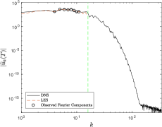
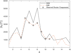
Figure 1: (a) The spectra of representative solutions of the DNS problem (black solid lines) and the LES problem (dashed red lines) together with the Fourier components whose real parts are recorded by the observation operators $H_{i}$, $i=1,\dots,8$, defined in Section 4.1.2, cf. (23) and (24b) (black circles). (b) Magnification of the wavenumber region around $k_{0}$. The green vertical line in panel (a) represents the cut-off wavenumber $k_{\text{max}}$. The DNS and LES problems (3) and (8) are solved numerically as described in Section 5.1.

5 Numerical Approach

The gradient-descent approach (13) is formulated in the continuous (“optimize-then-discretize”) setting [17] and evaluation of the gradient expression (18) requires solutions of the LES and the adjoint systems (8) and (19). In this section we first discuss the numerical solution of these PDE problems and the computation of the Sobolev gradients via (21)–(22). Then we describe the implementation of the gradient-descent algorithm (13).

5.1 Discretization

The LES and adjoint systems (8) and (19) involve model terms with state-dependent eddy viscosity $\nu(|{s}|)$ and in order to represent this expression, in addition to discretizing the space and time domains $[0,2\pi]$ and $[0,T]$, we also need to discretize the state domain $\mathcal{L}$. The former two domains are discretized using grids with equispaced points and steps sizes $\Delta x=2\pi/N_{x}$ and $\Delta t$, where $N_{x}$ is the number of grid points in space, whereas the state domain $\mathcal{L}$ is discretized with $N_{s}$ Chebyshev points. The original Kuramoto-Sivashinsky system (3), its LES version (8), and the adjoint system (19) are solved using the standard Fourier pseudo-spectral method [6] where dealiasing based on the 3/2 rule is performed in the case of the Kuramoto-Sivashinsky system (3), but due to aggressive filtering, cf. (4), is unnecessary in the latter two problems. Evaluation of the model terms in (8) and (19) requires differentiation of the eddy viscosity $\nu(|{s}|)$ with respect to ${s}$ which is performed using spectrally-accurate Chebyshev differentiation matrices [45] defined in the state domain $\mathcal{L}$. The eddy viscosity $\nu(|{s}|)$ and its derivative $d\nu(|{s}|)/d{s}$ are then interpolated from the state space to the physical space using the barycentric formulas which are also spectrally accurate [46]. This step ensures that the regularity required of the eddy viscosity, cf. (10), is maintained. The time-discretization of systems (3), (8), and (19) is performed using the exponential time-differencing fourth-order Runge-Kutta method (ETDRK4) [20], originally introduced in [7], which is fourth-order accurate. The different integrals are approximated using Gaussian quadratures, which are given by the trapezoidal rule on the periodic domain $\Omega$ (e.g., in (11)), and by the Clenshaw-Curtis formula on the bounded domain $\mathcal{L}$ (e.g., in (17)). The boundary-value problem (21)–(22) defining the Sobolev gradients is solved using the chebop feature of Chebfun [11], where the discretization is performed based on ultraspherical polynomials. With most computations carried out with spectral accuracy, approximation errors are dominated by time-stepping errors where the accuracy is $\mathcal{O}((\Delta t)^{4})$. Unless mentioned otherwise, in our computations we use $N_{x}={1024}$, $N_{s}={4096}$ and $\Delta t={3.0\times 10^{-6}}$.

In order to validate the discretization techniques discussed above, we verify the accuracy of the cost functional gradients evaluated as described in Section 3.1, cf. (18), by computing the Gâteaux differential $\mathcal{J}^{\prime}(\nu;\nu^{\prime})$ in terms of the Riesz identity (16) and comparing it with its approximation obtained with a simple forward finite-difference formula. The ratio of these two expressions is thus given by

$$\kappa(\epsilon):=\frac{\epsilon^{-1}\left[\mathcal{J}(\nu+\epsilon\nu^{\prime})-\mathcal{J}(\nu)\right]}{\left\langle\nabla_{{\nu}}^{L^{2}}\mathcal{J},\nu^{\prime}\right\rangle_{L^{2}(\mathcal{L})}},$$ (25)

where $\nu^{\prime}$ is an arbitrary perturbation and $\epsilon>0$ its magnitude. We expect $\kappa(\epsilon)$ to be close to unity and this is indeed evident in Figure 2 for a range of $\epsilon$ spanning several orders of magnitude. The large deviations of $\kappa(\epsilon)$ from unity observed for very small and very large values of $\epsilon$ are due to, respectively, the round-off and truncation errors in the finite-difference formula, both of which are well-known effects [4, 5]. In Figure 2 we also note that, as expected, for intermediate values of $\epsilon$, $\kappa(\epsilon)\rightarrow 1$ as the discretization parameter $\Delta t$ used in the numerical solution of the PDE systems (8) and (19) is refined. These results demonstrate the consistency of the cost functional gradients evaluated as discussed in Section 3.1 and also show that when sufficient numerical resolution is used, discretization errors will have a vanishing effect on the accuracy of the gradients and therefore also on the accuracy of the obtained optimal forms of the eddy viscosity. Thus, with the values of the discretization parameters $N_{x}$, $N_{s}$ and $\Delta t$ indicated above, our computations are fully resolved such that further refinements of these parameters would not produce appreciable changes of the results.

    

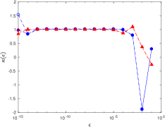
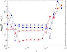
Figure 2: Dependence of 2 $\kappa$ and 2 $\log_{10}|1-\kappa|$ on $\epsilon$, cf. (25), for two different perturbations $\nu^{\prime}$ (blue circles vs. red triangles) and two different time steps (empty symbols) $\Delta t=3.0\times 10^{-6}$ and (filled symbols) $\Delta t=1.0\times 10^{-6}$ used in the solution of the PDE problems (8) and (19).

5.2 Gradient Descent

While for simplicity of presentation in Section 3 the steepest-descent (simple gradient) approach was used in (13), in actual computations we use the conjugate-gradients method [32] which is known to significantly accelerate convergence. The gradient $\nabla_{{\nu}}\mathcal{J}(\nu^{(n)})$ in (13) is then replaced with the descent direction $g^{(n)}$ defined as

$$g^{(n)} =\nabla_{{\nu}}\mathcal{J}(\nu^{(n)})-\gamma_{n}\,g^{(n-1)},\quad n=1,2,\dots,$$ (26)

$$g^{(0)} =\nabla_{{\nu}}\mathcal{J}(\nu^{(0)}),$$

where the “momentum” term $\gamma_{n}$ is evaluated using the Polak-Ribière formula

$$\gamma_{n}=\frac{\Big{\langle}\left(\nabla_{{\nu}}\mathcal{J}(\nu^{(n)})-\nabla_{{\nu}}\mathcal{J}(\nu^{(n-1)})\right),\nabla_{{\nu}}\mathcal{J}(\nu^{(n)})\Big{\rangle}_{H^{3}(\mathcal{L})}}{\Big{\langle}\nabla_{{\nu}}\mathcal{J}(\nu^{(n-1)}),\nabla_{{\nu}}\mathcal{J}(\nu^{(n-1)})\Big{\rangle}_{H^{3}(\mathcal{L})}}.$$ (27)

It is a good practice [32] for the conjugate-gradients approach (26) to be periodically restarted with a gradient step after a certain number of iterations. The line-minimization problem (14) is efficiently solved using Brent’s algorithm [36], which is a standard approach. Gradient iterations (13) are declared converged when the following termination condition is satisfied

$$\frac{|\mathcal{J}(\nu^{(n+1)})-\mathcal{J}(\nu^{(n)})|}{\mathcal{J}(\nu^{(n)})}<\epsilon_{\mathcal{J}},$$ (28)

where $\epsilon_{\mathcal{J}}$ is a prescribed tolerance (we will use $\epsilon_{\mathcal{J}}=10^{-7}$). The choice of the length-scale parameters $\ell_{1}$, $\ell_{2}$ and $\ell_{3}$ defining the Sobolev inner product (17b) will be discussed in the next section. The different steps in the solution of the optimization problem (12) are summarized as Algorithm 1.

Algorithm 1 Implementation of the conjugate-gradients variant of descent approach (13).
Input:
    $\{m(t)\}_{i=1}^{N}$ — target observations (e.g., of the DNS, cf. (3); $N$ is number of observations)
    $N_{x},N_{s},\Delta t$ — numerical discretization parameters
    $\ell_{1},\ell_{2},\ell_{3}$ — Sobolev length scales, cf. (17b)
    $\epsilon_{\mathcal{J}}$ — tolerance in the termination criterion (28)
    $\nu_{0}$ — initial guess for the eddy viscosity (e.g., (9))
Output:
    $\widecheck{\nu}$ — optimal eddy viscosity

• set $n=0$

• set $\nu^{(0)}=\nu_{0}$

repeat

     • set $n=n+1$

     • solve the LES problem (8)

     • solve the adjoint problem (19)

     • determine the $L^{2}$ gradient $\nabla_{\nu}^{L^{2}}\mathcal{J}(\nu^{(n)})$, cf. (18)

     • determine the Sobolev gradient $\nabla_{\nu}^{H^{3}}\mathcal{J}(\nu^{(n)})$ via (21)–(22)

     • determine the “momentum” coefficient $\gamma_{n}$ via (27)

     • determine the conjugate descent direction $g^{(n)}$ via (26)

     • determine the optimal step length $\tau^{(n)}$ by solving (14) with Brent’s algorithm

     • update the eddy viscosity $\nu^{(n)}\ \leftarrow\nu^{(n)}-\tau_{n}\,g^{(n)}$

until termination criterion (28) is satisfied

6 Results

In this section we present and analyze the results obtained with our approach to determining optimal eddy-viscosity closure models, cf. Algorithm 1, and compare them to the results obtained with other closure models including the approach of Das & Moser [9], where the closure model also has some optimality properties. We consider observation operators $H_{i}$, $i=1,\dots,N$, defined both in the physical space, cf. Section 4.1.1, and in the Fourier space, cf. Section 4.1.2, the latter with different distributions of the observed wavenumbers (24). With most other problem parameters fixed as discussed in Section 4.2, there remains one key characteristic defining the optimization problem (11)–(12), namely, the length of the time window and different values of $T$ are considered, covering from a few to several typical events in the evolution of the Kuramoto-Sivashinsky system (3) (these “events” are the merging of crests or formation on new ones). Summary information about these computations is compiled in Table 1, where we also indicate the values of the length-scale parameters $\ell_{2}$ and $\ell_{3}$ ($\ell_{1}=0$) used to determine the Sobolev gradients, cf. (17b). The values of these parameters are chosen by trial and error to maximize the convergence of iterations in Algorithm 1. We conclude from the data compiled in Table 1 that in all cases optimization reduces the observation error (11) by a factor $\mathcal{O}(1)$ with its specific value depending on the length of the optimization window $T$ and there tends to be an optimal value of $T$ for which the largest reduction of the error functional (11) is achieved. To fix attention, we will henceforth focus on two representative configurations, namely, one with observations in the physical space and one with observations in the Fourier space, denoted respectively “Case A” and “Case B” in Table 1.

Observations	Physical Space			Fourier Space — Equispaced			Fourier Space — Clustered
T	$1.5\times 10^{-3}$	$3.0\times 10^{-3}$	$9.0\times 10^{-3}$	$1.5\times 10^{-3}$	$3.0\times 10^{-3}$	$9.0\times 10^{-3}$	$1.5\times 10^{-3}$	$3.0\times 10^{-3}$	$9.0\times 10^{-3}$
${\ell_{2}}$	$10^{3}$	$10^{3}$	$10^{6}$	$10^{3}$	$10^{3}$	$10^{5}$	$10^{3}$	$10^{3}$	$10^{3}$
${\ell_{3}}$	$10^{1}$	$10^{1}$	$10^{5}$	$10^{1}$	$10^{1}$	$10^{5}$	$10^{1}$	$10^{1}$	$10^{1}$
${\frac{\mathcal{J}(\nu_{0})}{\mathcal{J}(\widecheck{\nu})}}$	$1.51$	$8.21$	$1.80$	$3.51$	$2.75$	$1.49$	$5.02$	$6.76$	$2.22$
Note		Case A						Case B

Table 1: Summary information about the different cases considered in our computations.

The decrease of the normalized objective functional (11) with iterations $n$ in Cases A and B is shown in Figure 3. In this figure we observe a reduction of the observation error by close to one order of magnitude over $\mathcal{O}(10)$ iterations. We note however that the convergence rate of iterations (13) is rather nonuniform. The corresponding optimal eddy viscosities $\widecheck{\nu}(s)$ are shown as functions of the resolved strain $s$ together with the Smagorinsky model (9) used as the initial guess in (13) in Figure 3. We see that while the optimal eddy viscosities $\widecheck{\nu}(s)$ are defined on a larger domain $\mathcal{L}$, the deviations from the initial guess $\nu_{0}$ produced by the gradient iterations (13) are essentially confined to a smaller identifiability interval $\mathcal{I}$. Most importantly, in contrast to the original Smagorinsky model (9), the optimal eddy viscosities are negative for small strains such that $\widecheck{\nu}(0)<0$. It is encouraging to note that the optimal eddy viscosities obtained in Cases A and B exhibit a qualitatively similar dependence on $s$, despite rather different forms of observations used to define the optimization problem (11)–(12) in these two cases.

    

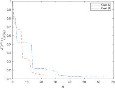
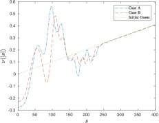
Figure 3: (a) Dependence of the normalized error functional $\mathcal{J}(\nu^{(n)})/\mathcal{J}(\nu_{0})$ on the iteration count $n$ and (b) dependence of the optimal eddy viscosity $\widecheck{\nu}({|s|})$ on the resolved strain $s$ for Case A (blue dash-dotted line) and Case B (red dashed line), cf. Table 1. In panel (b) we also indicate the Smagorinsky model (9) used as the initial guess $\nu_{0}$ (green dotted line).

In order to obtain insights about the spatio-temporal evolution of solutions to the LES problems (8) with different closure models (no closure at all, the Smagorinsky model (9), and the optimal eddy viscosity $\widecheck{\nu}({|s|})$ from Cases A and B, cf. Table 1), in Figure 4 these evolutions are compared as functions of space and time to the DNS solution $w(t,x)$ of the original Kuramoto-Sivashinsky system (3). In this figure we also include the evolution obtained with the optimal closure model proposed Das & Moser [9] based on a stochastic estimator. In order to assess the performance of the proposed approach at times $t>T$ extending beyond the “training window” $[0,T]$, the evolutions in Figure 4 are shown for $t\in[0,2T]$. We observe that with the exception of the LES solution with no closure model, cf. Figure 4, all LES solutions are qualitatively quite similar to the DNS solution, especially for short times, cf. Figures 4–4 vs. Figure 4, although the solutions obtained for Cases A and B arguably best correlate with the DNS results.

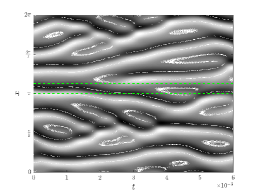
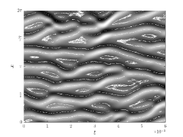
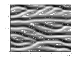
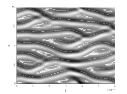
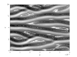
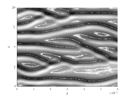
Figure 4: Space-time evolution of solutions to 4 the DNS problem (3) and the LES problems (8) with 4 no closure model, with 4 the Smagorinsky model (9), with 4 the optimal closure proposed by Das & Moser [9], with 4 the optimal closure from case A, and with 4 the optimal closure from case B. Grayscale indicates the solution value at given $(x,t)$. In panel 4 the green, dashed horizontal lines indicate the cut-off length scale $\delta$ characterizing filter (4).

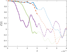
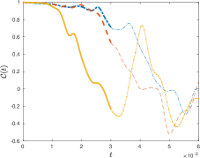
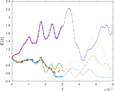
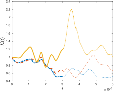
Figure 5: Dependence of the diagnostic quantities (a,b) $\mathcal{C}(t)$, cf. (29a), and (c,d) $\mathcal{K}(t)$, cf. (29b), on time $t$ for the LES solutions with (purple dot-dashed line) no closure model, with (green dotted line) the Smagorinsky model (9), with (blue dash-dotted line) the optimal eddy viscosity $\widecheck{\nu}$ from case A, with (red dashed line) the optimal eddy viscosity $\widecheck{\nu}$ from case B, and with (yellow solid-dotted line) the optimal closure proposed by Das & Moser [9]. Bold and thin lines correspond to time in the “training window” $t\in[0,T]$ and beyond the “training window” $t\in(T,2T]$, respectively.

To quantify these observations, we will now analyze the behavior of the following two diagnostic quantities

$$\mathcal{C}(t) :=\frac{1}{||w(t)||_{L^{2}(0,2\pi)}||\widetilde{u}(t)||_{L^{2}(0,2\pi)}}\int_{0}^{2\pi}w(t,x)\,\widetilde{u}(t,x)\ dx,$$ (29a)

$$\mathcal{K}(t) :=\frac{||\widetilde{u}(t)||^{2}_{L^{2}(0,2\pi)}}{||w(t)||^{2}_{L^{2}(0,2\pi)}}=\frac{1}{||w(t)||^{2}_{L^{2}(0,2\pi)}}\,\int^{2\pi}_{0}\widetilde{u}(t,x)^{2}\,dx,$$ (29b)

which can be interpreted as, respectively, the correlation of the LES solution $\widetilde{u}$ with the DNS solution $w$ and the normalized kinetic energy. The LES with the optimal eddy-viscosity closures obtained in Cases A and B are compared in terms these diagnostic quantities for $t\in[0,2T]$ to the LES with no closure model, with the Smagorinsky model (9), and with the closure model of Das & Moser [9] in Figure 5. Given the chaotic nature of the Kuramoto-Sivashinsky system (3) resulting in an exponentially fast divergence of initially nearby trajectories, in all cases the correlation (29a) drops very rapidly, such that for short times $t\rightarrow 0$ we approximately have $\mathcal{C}(t)\approx 1-r\,e^{pt}$ for some $r,p>0$ different in each case, cf. Figures 5(a). The growth rate $p$, characterizing the exponential divergence of the solutions to the DNS and LES problems, is smallest when the optimal eddy-viscosity closure models $\widecheck{\nu}(|s|)$ from cases A and B are used. As a result, the time $t_{0}$ when the DNS and the LES solutions become uncorrelated, i.e., when $\mathcal{C}(t_{0})\approx 0$, is nearly twice as large for the optimal eddy-viscosity closures from Cases A and B than for the Smagorinsky model (9) and the closure model of Das & Moser [9]. As regards the behavior of the normalized energy (29b), from Figures 5–5 we see that the optimal eddy viscosity $\widecheck{\nu}({|s|})$ on average tends to reduce the kinetic energy relative to its levels in the DNS. This is in contrast to the approach of Das & Moser [9] in which the normalized energy is increased to levels higher than in the DNS, cf. Figure 5.

While the analysis above focused on “a posteriori” tests involving the results of solving the LES system (8) with different closure models, we close this section with a brief discussion of an “a priori” test where the errors in approximations of the SGS stresses (6) with different closure models are analyzed. In this context, comparing the SGS dissipation rate with the modeled SGS dissipation rate is often used as a standard diagnostic to assess the energetics in the LES flow [30]. We thus focus on the following normalized least-squares measure of this error

$$\mathcal{S}(t):=\frac{1}{||\frac{\partial\widetilde{u}}{\partial x}\,M(t)||^{2}_{L^{2}(0,2\pi)}}\int_{0}^{2\pi}\left[\frac{\partial\widetilde{u}}{\partial x}\left[M(w(t,x))-M(\widetilde{u}(t,x))\right]\right]^{2}\ dx$$ (30)

and show its dependence on time $t\in[0,2T]$ for different models in Figure 6. We note in this figure that the normalized SGS stress error $\mathcal{S}(t)$ tends to be quite large in all cases, which is a known property of Smagorinsky-type models [15], and is smallest in the case of Das’ & Moser’s approach [9].

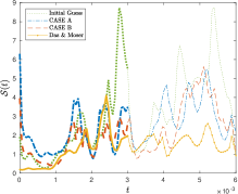
Figure 6: Dependence of the normalized SGS stress error $\mathcal{S}(t)$, cf. (30), on time $t$ for the LES solutions with (green dotted line) the Smagorinsky model (9), with (blue dash-dotted line) the optimal eddy viscosity $\widecheck{\nu}$ from case A, with (red dashed line) the optimal eddy viscosity $\widecheck{\nu}$ from case B, and with (yellow solid-dotted line) the optimal closure proposed by Das & Moser [9]. Bold and thin lines correspond to time in the “training window” $t\in[0,T]$ and beyond the “training window” $t\in(T,2T]$, respectively.

7 Discussion and Conclusions

In this study we have introduced a computational framework for determining optimal eddy-viscosity closures for a broad class of PDE models, such as the Navier-Stokes equation in hydrodynamics. This inverse problem is framed here as a PDE optimization problem where an error functional representing the misfit between the target and predicted observations is minimized with respect to the functional form of the eddy viscosity in the closure relation which determines the “shape” of the nonlinearity of the model term. Because of this latter aspect, such a problem is not amenable to solution using standard adjoint-based tools for PDE optimization and an extension of the recently developed generalization of these techniques [4, 5] needs to be used. In addition, by formulating the problem in the “optimize-then-discretize” setting we are able to determine the optimal forms of the eddy viscosity in a very general manner subject only to some minimal assumptions on smoothness, cf. (10), and the behavior for small and large values of the state variable. Solution of this problem using a “discretize-then-optimize” approach often employed to solve PDE optimization problems [17] is an interesting alternative. Such formulations ought to be contrasted with some earlier approaches in which optimal closures were determined by fitting a small number of parameters in an assumed ansatz. Thus, our proposed approach does not suffer from the limitations of such an assumed ansatz.

To provide a proof of the concept for this approach, we have focused here on the 1D Kuramoto-Sivashinsky equation (3) as a model problem computationally more tractable than the 2D or 3D Navier-Stokes system we are ultimately interested in. In being chaotic and multiscale [18], the solutions of the Kuramoto-Sivashinsky system arguably better resemble actual hydrodynamic turbulence than solutions of the Burgers equation often used as a simplified model in similar situations [9]. Such simplified setting allows us to study the properties of our proposed approach more thoroughly. We find that it is possible to determine a particular dependence of the eddy viscosity on the resolved strain, $\widecheck{\nu}=\widecheck{\nu}(|s|)$, generalizing Smagorinsky’s relation (9) in a LES model, such that the LES model provides a systematically improved approximation of the DNS. More precisely, while the trajectories corresponding to the DNS and LES still diverge exponentially, they do so at a much slower rate than in the case of the LES based on the standard Smagorinsky model, cf. Figure 5(a). Importantly, the functional form of the optimal eddy viscosity $\widecheck{\nu}(|s|)$ appears to little depend on the particular form of the observations used to set up the optimization problem, cf. Figure 3, and we emphasize here that our approach can be formulated based on very general measurements (changing the observation operator $H_{i}$, cf. Section 4.1, will only result in a modification of the source term in the adjoint system (19a)). In particular, it is also possible to simultaneously use several different sets of measurements coming, for example, from different DNS or experiments, and a natural way to formulate such a problem is in terms of multiobjective optimization.

The LES with the optimal eddy-viscosity closure models determined with the proposed approach produces solutions which better match the DNS than the LES solutions obtained with the closure model of Das & Moser [9], cf. Figure 5(b). On the other hand, that latter model leads to a more accurate prediction of the SGS stresses, cf. Figure 6. This can be understood by recognizing that the closure model of Das & Moser is formulated to optimally reconstruct the SGS stresses rather than some other a posteriori quantities. We have also considered a formulation with observation operators involving SGS stresses, but the results obtained were inferior to the results presented here. In our computations the numerical parameters $N_{x}$, $N_{s}$ and $\Delta t$ were chosen such that the LES and the adjoint systems (8) and (19), the gradient expression (18) as well as the system (21)–(22) for determining the Sobolev gradients were fully resolved, cf. Section 5.1. The effect of insufficient numerical resolution on the computed optimal eddy-viscosity closures is an important question which merits investigation, however, the answer will likely be problem dependent.

In addition to providing optimal eddy-viscosity closure models which can be useful in many situations, the present approach serves another, more basic purpose, namely, by identifying the “best” closure models within a certain family it can offer information about their fundamental performance limitations. More specifically, it can provide insights about how well closure models based on the eddy-viscosity ansatz (2) can perform in the best case and thus how much room there is in principle for improvement of standard approaches such as the Smagorinsky model (9).

Moving forward, our next main goal is to consider an analogous problem of finding optimal eddy-viscosity closure models for the 2D and 3D Navier-Stokes system as generalizations of the Smagorinsky model (2), first in the periodic setting and then in more realistic geometries. In that latter context related questions also arise as regards wall models. We are also interested in studying closure models based on formulations other than eddy viscosity.

Appendix A Proof of Theorem 1

Here we derive expression (18) for the $L^{2}$ gradient of the cost functional (11). In order to avoid technical complications related to the non-differentiability of the absolute value $|\cdot|$ in the argument of the eddy viscosity, we change the variable from $|s|$ to $\sigma:=|s|^{2}=s^{2}$ (for simplicity and with a slight abuse of notations we will still use the same symbol $\nu=\nu(\sigma)$ to denote the eddy viscosity). First, we must determine the perturbation of the LES system (8) resulting from perturbing the functional form of the eddy viscosity $\nu$ with some perturbation $\nu^{\prime}$. This is done by replacing $\widetilde{u}$ and $\nu$ with the following representations in which $0<\epsilon\ll 1$

$$\widetilde{u}\ \ \longleftarrow\widetilde{u}+\epsilon\,\widetilde{u}^{\prime}+\mathcal{O}(\epsilon^{2}),$$ (31a)

$$\nu(\sigma)\ \ \longleftarrow\nu(\sigma)+\epsilon\,\frac{d\nu(\sigma)}{d\sigma}\frac{d\sigma}{ds}\frac{\partial\widetilde{u}^{\prime}}{\partial x}+\epsilon\,\nu^{\prime}(\sigma)+\mathcal{O}(\epsilon^{2}).$$ (31b)

The second term on the RHS in (31b) reflects the change of the value of the (squared) strain $\sigma$ for which the eddy viscosity is evaluated as a result of perturbing its functional form [4, 5]. Substituting representations (31a)–(31b) into the LES system (8) and collecting terms of $\mathcal{O}(\epsilon)$ we obtain the following perturbation system

$$\frac{\partial\widetilde{u}^{\prime}}{\partial t}+\nu_{4}\,\frac{\partial^{4}\widetilde{u}^{\prime}}{\partial x^{4}}+\nu_{2}\Big{[}\frac{\partial^{2}\widetilde{u}^{\prime}}{\partial x^{2}}+\frac{\partial{(\widetilde{u}\widetilde{u}^{\prime})}}{\partial x}\Big{]} +\frac{\partial}{\partial x}\Big{[}\frac{d\nu(\sigma)}{d\sigma}\frac{d\sigma}{ds}\frac{\partial^{3}\widetilde{u}}{\partial x^{3}}\frac{\partial\widetilde{u}^{\prime}}{\partial x}+\nu\,\frac{\partial^{3}\widetilde{u}^{\prime}}{\partial x^{3}}\Big{]}=-\frac{\partial}{\partial x}\Big{[}\nu^{\prime}\frac{\partial^{3}\widetilde{u}}{\partial x^{3}}\Big{]},$$ (32a)

$$\frac{\partial^{(i)}\widetilde{u}^{\prime}}{\partial x^{(i)}}(t,0) =\frac{\partial^{(i)}\widetilde{u}^{\prime}}{\partial x^{(i)}}(t,2\pi),\quad\quad i=0,\dotsc,3,$$ (32b)

$$\widetilde{u}^{\prime}(0,x) =0$$ (32c)

describing the leading-order effect $\widetilde{u}^{\prime}$ of perturbing the functional form of the eddy viscosity $\nu(\sigma)$ on solutions of the LES system (8) [4, 5]. Now we integrate (32a) against the adjoint field $\widetilde{u}^{*}$ over the space-time domain $[0,2\pi]\times[0,T]$ and then perform integration by parts with respect to both space and time to obtain

$$0=\int_{0}^{T}\int_{0}^{2\pi}\bigg{[}\frac{\partial\widetilde{u}^{\prime}}{\partial t}+\nu_{4}\,\frac{\partial^{4}\widetilde{u}^{\prime}}{\partial x^{4}}+\nu_{2}\Big{[}\frac{\partial^{2}\widetilde{u}^{\prime}}{\partial x^{2}}+\frac{\partial{(\widetilde{u}\,\widetilde{u}^{\prime})}}{\partial x}\Big{]}\bigg{]}\,\widetilde{u}^{*}\,dx\,dt$$

$$\ \ +\int_{0}^{T}\int_{0}^{2\pi}\frac{\partial}{\partial x}\bigg{[}\frac{d\nu}{d\sigma}\,\frac{d\sigma}{ds}\,\frac{\partial^{3}\widetilde{u}}{\partial x^{3}}\,\frac{\partial\widetilde{u}^{\prime}}{\partial x}+\nu\,\frac{\partial^{3}\widetilde{u}^{\prime}}{\partial x^{3}}+\nu^{\prime}\,\frac{\partial^{3}\widetilde{u}}{\partial x^{3}}\ \bigg{]}\,\widetilde{u}^{*}\,dx\,dt$$

$$= \underbrace{\int_{0}^{T}\int_{0}^{2\pi}\left[-\frac{\partial\widetilde{u}^{*}}{\partial t}+\nu_{4}\frac{\partial^{4}\widetilde{u}^{*}}{\partial x^{4}}+\nu_{2}\left[\frac{\partial^{2}\widetilde{u}^{*}}{\partial x^{2}}-\widetilde{u}\frac{\partial\widetilde{u}^{*}}{\partial x}\right]+\frac{\partial}{\partial x}\left[\frac{d\nu}{d\sigma}\frac{d\sigma}{ds}\frac{\partial^{3}\widetilde{u}}{\partial x^{3}}\frac{\partial\widetilde{u}^{*}}{\partial x}\right]+\frac{\partial^{3}}{\partial x^{3}}\left[\nu\frac{\partial\widetilde{u}^{*}}{\partial x}\right]\right]\,\widetilde{u}^{\prime}\,dx\,dt}_{\mathcal{J}^{\prime}(\nu;\nu^{\prime})}$$

$$-\int_{0}^{T}\int_{0}^{2\pi}\frac{\partial\widetilde{u}^{*}}{\partial x}\,\frac{\partial^{3}\widetilde{u}}{\partial x^{3}}\,\nu^{\prime}\,dx\,dt=0,$$

where all the boundary terms vanish due to periodicity. Using the definition of the adjoint system (19) together with the aforementioned change of variables $\sigma=\sigma(s)$ we then obtain for the Gâteaux differential $\mathcal{J}^{\prime}(\nu;\nu^{\prime})=\int_{0}^{T}\int_{0}^{2\pi}\frac{\partial\widetilde{u}^{*}}{\partial x}\,\frac{\partial^{3}\widetilde{u}}{\partial x^{3}}\,\nu^{\prime}\,dx\,dt$, which now contains the perturbation $\nu^{\prime}$ as a factor, but is still not in the Riesz form (16) because this form involves an inner product defined with integration with respect to the resolved strain $s$ rather than space $x$ and time $t$ (we shall now return back to the original variable via the substitution $\sigma=s^{2}$). The required change of variables is introduced by the representation [4, 5] $\nu^{\prime}\Big{(}\Big{|}\frac{\partial\widetilde{u}(t,x)}{\partial x}\Big{|}\Big{)}=\int_{a}^{b}\delta\Big{(}\Big{|}\frac{\partial\widetilde{u}(t,x)}{\partial x}\Big{|}-s\Big{)}\,\nu^{\prime}(s)\,ds$, where $\delta(\cdot)$ is the Dirac delta distribution, such that using Fubini’s theorem to swap the order of integration we finally arrive at a Riesz representation of the Gâteaux differential (3.1)

$$\mathcal{J}^{\prime}(\nu;\nu^{\prime}) =\int_{0}^{T}\int_{0}^{2\pi}\frac{\partial\widetilde{u}^{*}(t,x)}{\partial x}\,\int_{a}^{b}\delta\Big{(}\Big{|}\frac{\partial\widetilde{u}(t,x)}{\partial x}\Big{|}-s\Big{)}\,\frac{\partial^{3}\widetilde{u}(t,x)}{\partial x^{3}}\,\nu^{\prime}(s)\,ds\,dx\,dt$$

$$=\int_{a}^{b}\left[\int_{0}^{T}\int_{0}^{2\pi}\frac{\partial\widetilde{u}^{*}(t,x)}{\partial x}\,\delta\Big{(}\Big{|}\frac{\partial\widetilde{u}(t,x)}{\partial x}\Big{|}-s\Big{)}\,\frac{\partial^{3}\widetilde{u}(t,x)}{\partial x^{3}}\,dx\,dt\right]\nu^{\prime}(s)\,ds,$$ (33)

from which after selecting $\mathcal{X}=L^{2}(\mathcal{L})$ in (16) we deduce the following expression for the $L^{2}$ gradient

$$\nabla_{\nu}^{L^{2}}\mathcal{J}(s)=\int_{0}^{T}\int_{0}^{2\pi}\frac{\partial\widetilde{u}^{*}(t,x)}{\partial x}\,\delta\Big{(}\Big{|}\frac{\partial\widetilde{u}(t,x)}{\partial x}\Big{|}-s\Big{)}\,\frac{\partial^{3}\widetilde{u}(t,x)}{\partial x^{3}}\,dx\,dt.$$ (34)

We note that evaluation of this expression for a given value of $s$ requires computation of an integral defined on the level set $\Big{|}\frac{\partial\widetilde{u}(t,x)}{\partial x}\Big{|}=s$ in the space-time domain $[0,2\pi]\times[0,T]$ which is rather difficult. A computationally more convenient approach is obtained using the following identity (in which the differentiation is understood in the distributional sense) $\delta\Big{(}\Big{|}\frac{\partial\widetilde{u}(t,x)}{\partial x}\Big{|}-s\Big{)}=-\frac{d}{ds}{\Xi}_{\left[\alpha,\big{|}\partial\widetilde{u}(t,x)/\partial x\big{|}\right]}(s)$, such that (34) becomes

$$\nabla_{\nu}^{L^{2}}\mathcal{J}(s)=-\frac{d}{ds}\int_{0}^{T}\int_{0}^{2\pi}{\Xi}_{\left[\alpha,\big{|}\frac{\partial\widetilde{u}(t,x)}{\partial x}\big{|}\right]}(s)\,\frac{\partial\widetilde{u}^{*}(t,x)}{\partial x}\,\frac{\partial^{3}\widetilde{u}(t,x)}{\partial x^{3}}\,dx\,dt,$$ (35)

and expression (18) is finally obtained.

References

- [1] R. A. Adams and J. F. Fournier, Sobolev Spaces, vol. 140 of Pure and Applied Mathematics (Amsterdam), Elsevier/Academic Press, Amsterdam, 2nd ed., 2003.
- [2] J. Bec and K. Khanin, Burgers turbulence, Phys. Rep., 447 (2007), pp. 1–66.
- [3] M. S. Berger, Nonlinearity and Functional Analysis, Academic Press, 1977.
- [4] V. Bukshtynov and B. Protas, Optimal reconstruction of material properties in complex multiphysics phenomena, J. Comput. Phys., 242 (2013), pp. 889–914.
- [5] V. Bukshtynov, O. Volkov, and B. Protas, On optimal reconstruction of constitutive relations, Phys. D, 240 (2011), pp. 1228–1244.
- [6] C. Canuto, M. Y. Hussaini, A. Quarteroni, and T. A. Zang, Spectral Methods in Fluid Dynamics, Springer-Verlag, Berlin, 1988.
- [7] S. M. Cox and P. C. Matthews, Exponential time differencing for stiff systems, J. Comput. Phys., 176 (2002), pp. 430–455.
- [8] I. Danaila and B. Protas, Optimal reconstruction of inviscid vortices, Proceedings of the Royal Society A, 471 (2015), 20150323.
- [9] A. Das and R. D. Moser, Optimal large-eddy simulation of forced Burgers equation, Phys. Fluids, 14 (2002), pp. 4344–4351.
- [10] P. A. Davidson, Turbulence: An introduction for scientists and engineers, Oxford University Press, Oxford, 2nd ed., 2015.
- [11] T. A. Driscoll, N. Hale, and L. N. Trefethen, Chebfun Guide, Pafnuty Publications, Oxford, UK, 2014.
- [12] K. Duraisamy, G. Iaccarino, and H. Xiao, Turbulence Modeling in the Age of Data, Annu. Rev. Fluid Mech., 51 (2019), pp. 357–377.
- [13] P. A. Durbin, Some Recent Developments in Turbulence Closure Modeling, Annu. Rev. Fluid Mech., 50 (2018), pp. 77–103.
- [14] U. Frisch, Turbulence, Cambridge University Press, Cambridge, 1995. The legacy of A. N. Kolmogorov.
- [15] M. Gamahara and Y. Hattori, Searching for turbulence models by artificial neural network, Phys. Rev. Fluids, 2 (2017), 054604.
- [16] M. Germano, Turbulence: the filtering approach, J. Fluid Mech., 238 (1992), pp. 325–336.
- [17] M. D. Gunzburger, Perspectives in Flow Control and Optimization, SIAM, 2003.
- [18] P. Holmes, J. L. Lumley, G. Berkooz, and C. W. Rowley, Turbulence, Coherent Structures, Dynamical Systems and Symmetry, Cambridge Monogr. Mech., Cambridge University Press, Cambridge, 2nd ed., 2012.
- [19] J. Jimenez, Machine-aided turbulence theory, J. Fluid Mech., 854 (2018), R1.
- [20] A. Kassam and L. N. Trefethen, Fourth-Order Time-Stepping for Stiff PDEs, SIAM J. Sci. Comput., 26 (2005), pp. 1214–1233.
- [21] Y. Kuramoto, Diffusion-Induced Chaos in Reaction Systems, Progress of Theoretical Physics Supplement, 64 (1978), pp. 346–367.
- [22] J. N. Kutz, Deep learning in fluid dynamics, J. Fluid Mech., 814 (2017), pp. 1–4.
- [23] J. A. Langford and R. D. Moser, Optimal LES formulations for isotropic turbulence, J. Fluid Mech., 398 (1999), pp. 321–346.
- [24] M. Lesieur and O. Metais, New Trends in Large-Eddy Simulations of Turbulence, Annu. Rev. Fluid Mech., 28 (1996), pp. 45–82.
- [25] D. K. Lilly, A proposed modification of the Germano subgrid-scale closure method, Physics of Fluids A: Fluid Dynamics, 4 (1992), pp. 633–635.
- [26] J. Ling, A. Kurzawski, and J. Templeton, Reynolds averaged turbulence modelling using deep neural networks with embedded invariance, J. Fluid Mech., 807 (2016), pp. 155–166.
- [27] J. Lions, Contrôle Optimal de Systèmes Gouvernés par des Équations aux Dérivées Partielles, Dunod, Paris, 1968. (English translation, Springer-Verlag, New-York (1971)).
- [28] D. Luenberger, Optimization by Vector Space Methods, John Wiley and Sons, 1969.
- [29] R. Maulik, O. San, A. Rasheed, and P. Vedula, Data-driven deconvolution for large eddy simulations of kraichnan turbulence, Physics of Fluids, 30 (2018), 125109.
- [30] C. Meneveau, Statistics of turbulence subgrid‐scale stresses: Necessary conditions and experimental tests, Physics of Fluids, 6 (1994), pp. 815–833.
- [31] J. Neuberger, Sobolev Gradients and Differential Equations, Springer, 2010.
- [32] J. Nocedal and S. Wright, Numerical Optimization, Springer Series in Operations Research and Financial Engineering, Springer, 2nd ed., 2006.
- [33] S. Pan and K. Duraisamy, Data-driven discovery of closure models, SIAM J. Appl. Dyn. Syst., 17 (2018), pp. 2381–2413.
- [34] E. J. Parish and K. Duraisamy, A paradigm for data-driven predictive modeling using field inversion and machine learning, J. Comput. Phys., 305 (2016), pp. 758 – 774.
- [35] S. B. Pope, Turbulent flows, Cambridge University Press, Cambridge, 2000.
- [36] W. H. Press, S. A. Teukolsky, W. T. Vetterling, and B. P. Flannery, Numerical Recipes 3rd Edition: The Art of Scientific Computations, Cambridge University Press, 2007.
- [37] B. Protas, T. R. Bewley, and G. Hagen, A computational framework for the regularization of adjoint analysis in multiscale PDE systems, Journal of Computational Physics, 195 (2004), pp. 49 – 89.
- [38] B. Protas, B. R. Noack, and M. Morzyński, An Optimal Model Identification For Oscillatory Dynamics With a Stable Limit Cycle, J. Nonlin. Sci., 24 (2014), pp. 245–275.
- [39] B. Protas, B. R. Noack, and J. Östh, Optimal nonlinear eddy viscosity in Galerkin models of turbulent flows, J. Fluid Mech., 766 (2015), pp. 337–367.
- [40] W. Rodi, G. Constantinescu, and T. Stoesser, Large-Eddy Simulation in Hydraulics, CRC Press, 2013.
- [41] P. Sagaut, Large Eddy Simulation for Incompressible Flow, Sci. Comput., Springer-Verlag, Berlin, 3rd ed., 2006.
- [42] A. K. Sethurajan, S. A. Krachkovskiy, I. C. Halalay, G. R. Goward, and B. Protas, Accurate Characterization of Ion Transport Properties in Binary Symmetric Electrolytes Using In Situ NMR Imaging and Inverse Modeling, The Journal of Physical Chemistry B, 119 (2015), pp. 12238–12248.
- [43] G. I. Sivashinsky, Nonlinear analysis of hydrodynamic instability in laminar flames. I. Derivation of basic equations, Acta Astronaut., 4 (1977), pp. 1177–1206.
- [44] J. Smagorinsky, General circulation experiments with the primitive equations: I. The basic experiment, Monthly weather review, 91 (1963), pp. 99–164.
- [45] L. N. Trefethen, Spectral Methods in MATLAB, SIAM, Philadelphia, 2000.
- [46] L. N. Trefethen, Approximation Theory and Approximation Practice, SIAM, Philadelphia, 2013.
- [47] X. Xie, M. Mohebujjaman, L. Rebholz, and T. Iliescu, Data-driven filtered reduced order modeling of fluid flows, SIAM J. Sci. Comput., 40 (2018), pp. B834–B857.