Interacting kinks and meson mixing

Abstract

A Rayleigh-Schrödinger type of perturbation scheme is employed to study weakly interacting kinks and domain walls formed from two different real scalar fields $\chi$ and $\varphi$. An interaction potential $V_{1}(\chi,\varphi)$ is chosen which vanishes in a vacuum state of either field. Approximate first order corrections for the fields are found, which are associated with scalar field condensates inhabiting the zeroth order topological solitons. The model considered here presents several new and interesting features. These include (1) a condensate of each kink field inhabits the other kink, (2) the condensates contribute an associated mass to the system which vanishes when the kinks overlap, (3) a resulting mass defect of the system for small interkink distances allows the existence of a loosely bound state when the interkink force is repulsive. An identification of the interaction potential energy and forces allows a qualitative description of the classical motion of the system, with bound states, along with scattering states, possible when the interkink force is attractive. (4) Finally, the interaction potential introduces a mixing and oscillation of the perturbative $\chi$ and $\varphi$ meson flavor states, which has effects upon meson-kink interactions.

I Introduction

It has been long recognized that certain nonlinear field theories possessing multiple disconnected vacuum states admit, in addition to a set of perturbative particle spectra, additional states associated with the topology of the vacuum manifold (see, e.g., Goldstone75 ,Jackiw77 , and references therein). These nonperturbative states, or “solitons”, typically have nontrivial internal structures that can depend upon one or more spatial dimensions (see, e.g., Goldstone75 -KTbook ). Studies of one dimensional topological defects, describing “kinks”, or planar domain walls can expose interesting properties of solitons and their interactions with other solitons and ordinary matter. In addition, the one dimensional defects can be described by sets of simpler differential equations that depend only upon one space variable. In addition, much attention has been given to investigations involving various interactions between scalar fields describing kinks of more than one variety, which can arise from models involving two distinct scalar fields. (For a sample of such types of analyses see, for example, Baz PLA13 -Alfonso PRD07 .)

Here, a fairly simple model describing two weakly interacting scalar fields, denoted by $\chi$ and $\varphi$, is presented which exhibits some new and interesting features. A potential $V(\chi,\varphi)=V_{0}(\chi,\varphi)+V_{1}(\chi,\varphi)$ is chosen which admits solutions describing interacting $\phi^{4}$-type kink solutions in a $1+1$ dimensional spacetime (or planar domain walls in higher dimensional spacetimes. These are simply referred to here as “kinks” for simplicity (see, e.g., Goldstone75 -KTbook )). The unperturbed potential is given by $V_{0}(\chi,\varphi)=\frac{1}{4}\lambda_{\chi}\left(\chi^{2}-\eta^{2}\right)^{2}+\frac{1}{4}\lambda_{\varphi}\left(\varphi^{2}-\sigma^{2}\right)^{2}$ and the interaction potential is chosen to be $V_{1}(\chi,\varphi)=\frac{1}{2}\beta\left(\chi^{2}-\eta^{2}\right)\left(\varphi^{2}-\sigma^{2}\right)$ where the parameter $\beta$ is small in comparison to $\lambda_{\chi}$ or $\lambda_{\varphi}$, i.e., $|\beta|\ll\lambda$. When $\beta=0$ the model admits the familiar tanh - like solutions describing $\chi$ and $\varphi$ kinks and antikinks, and when the interaction is turned on with $\beta\neq 0$ the $\chi$ and $\varphi$ kinks interact with each other. We allow the nonvanishing $\beta$ to be either positive or negative, allowing for either repulsive or attractive interactions between the $\chi$ and $\varphi$ kinks. We note that $V_{1}$ vanishes in the vacuum state of either field, where $\chi_{\text{vac}}=\pm\eta$ and $\varphi_{\text{vac}}=\pm\sigma$, i.e., the vacuum states are preserved by the interaction.

The addition of a perturbing potential necessitates corrections to the $\tanh kx$ kink solutions of the unperturbed theory. (See, for example, Deform -Defect13 and DB96 ,DB97 .) Here, a basic Rayleigh-Schrödinger type of perturbation scheme is developed to obtain equations describing a set of corrections $\left\{\chi_{n},\varphi_{n}\right\}$ to the unperturbed base solutions $\chi_{0},\varphi_{0}$. We focus upon the first order static corrections $\chi_{1}(x)$ and $\varphi_{1}(x)$, each of which satisfies a nonhomogeneous linear differential equation (DE) involving hyperbolic functions. Failing to find exact analytical solutions to these equations, we instead obtain approximate analytical solutions using a type of “thin wall” approximation. These approximate analytical solutions have the advantage of displaying the roles of the various model parameters, such as the widths $w_{\chi}$ and $w_{\varphi}$ of the kinks and the separation distance $a$ between them. These solutions are useful in obtaining subsequent features of the model. Although the approximation is expected to work better for massive, narrow width kinks, it is expected to exhibit, at least, the qualitative behaviors of less massive, wider, kinks as well.

The first order corrections for this model yield some surprising results, some of which may apply to other two-field models, as well. (1) One surprising result is that the static first order corrections, which are associated with scalar field condensates, have the peculiar character that they are pronounced at the locations of the $\chi_{0}$ and $\varphi_{0}$ kinks. More specifically, the condensate of each kink field inhabits the other kink. That is, $\chi_{1}(x)$ becomes localized at the location of the $\varphi_{0}$ kink, and $\varphi_{1}(x)$ is localized at the location of the $\chi_{0}$ kink. These localized corrections, or “displaced scalar field condensates”, are nontopological and essentially inhabit the zeroth order kinks. The combination of a soliton with a scalar field condensate then comprises a “structured” kink.

(2) The approximate “mass” associated with each condensate is found, which contributes to the total mass of the structured kink. A distinctive property of the structured kinks is that the mass associated with a condensate decreases with separation distance between the kinks when they are close together, and the condensate mass vanishes when the kinks overlap, i.e., occupy the same position. (3) The resulting “mass defect”, or “binding energy”, connected with the condensate masses therefore allows the existence of a loosely bound state of the $\chi$ and $\varphi$ kinks when the interkink force is repulsive.

Using the base solutions for the static kinks, a classical potential energy of interaction, along with an interaction force between the kinks, can be defined, allowing a qualitative description of the classical motion of the system. The interaction force can be either attractive ($\beta<0$) or repulsive ($\beta>0$).  When the interkink force is attractive, stronger bound states can exist, giving rise to composite two-kink states of the $(\chi,\varphi)$ system. These composite states can have topological charges of $Q=\pm 2$ or $0$.

(4) Finally, it is pointed out that an interaction between the $\chi$ and $\varphi$ fields produces a nondiagonal mass matrix for the perturbative “meson” flavor states $|\chi\rangle$ and $|\varphi\rangle$ that are built from the vacuum states $\chi_{\text{vac}}=\pm\eta$ and $\varphi_{\text{vac}}=\pm\sigma$. Therefore, the flavor states $|\chi\rangle$ and $|\varphi\rangle$ are combinations of mass eigenstates $|\phi_{1}\rangle$ and $|\phi_{2}\rangle$, resulting in oscillations of the $\chi$ and $\varphi$ scalar particles. Since only $\chi$ ($\varphi$) particles reflect from a $\varphi$ ($\chi$) kink, the radiative force exerted on one kink due to scalar radiation from the other kink will be affected by the oscillations.

Computational details for several results are relegated to Appendices.

II The Model

We take the Lagrangian of real-valued scalar fields $\chi$ and $\varphi$ to be

$$\mathcal{L}=\frac{1}{2}(\partial\chi)^{2}+\frac{1}{2}(\partial\varphi)^{2}-V(\chi,\varphi),\ \ \ \ \ V(\chi,\varphi)=V_{0}(\chi,\varphi)+V_{1}(\chi,\varphi)$$ (1)

with $V_{1}$ acting as a small perturbation to $V_{0}$, where

$$\begin{array}[]{ll}&V_{0}(\chi,\varphi)=\frac{1}{4}\lambda_{\chi}\left(\chi^{2}-\eta^{2}\right)^{2}+\frac{1}{4}\lambda_{\varphi}\left(\varphi^{2}-\sigma^{2}\right)^{2}\\ &V_{1}(\chi,\varphi)=\frac{1}{2}\beta\left(\chi^{2}-\eta^{2}\right)\left(\varphi^{2}-\sigma^{2}\right)\end{array}$$ (2)

where the coupling constants $\lambda_{\chi}$ and $\lambda_{\varphi}$ are positive, and $\beta$ can be either positive or negative. When $V_{1}=0$ the equations of motion support the familiar $\phi^{4}$ type of kink/domain wall solutions. The $\frac{1}{2}\beta\chi^{2}\varphi^{2}$ term is an interaction term and $V_{1}$ is considered to be a small perturbation with $|\beta|\ll\lambda_{\chi},\lambda_{\varphi}$.

The equations of motion are given by $\square\chi+\partial_{\chi}V(\chi,\varphi)=0$ and$\ \square\varphi+\partial_{\varphi}V(\chi,\varphi)=0$, or, more specifically, by

$$\square\chi+\lambda_{\chi}\chi(\chi^{2}-\eta^{2})+\beta\chi(\varphi^{2}-\sigma^{2}) =0,$$ (3a)

$$\ \ \ \square\varphi+\lambda_{\varphi}\varphi(\varphi^{2}-\sigma^{2})+\beta\varphi(\chi^{2}-\eta^{2}) =0$$ (3b)

where $\square=\partial_{t}^{2}-\nabla^{2}$ and $\partial_{\chi}=\partial/\partial\chi$, $\partial_{\varphi}=\partial/\partial\varphi$, etc. The vacuum states are $\chi_{\text{vac}}=\pm\eta$ and $\varphi_{\text{vac}}=\pm\sigma$.

In the absence of interaction ($\beta=0$) the system admits static kink solutions $\chi_{0}(x)=\eta\tanh k_{\chi}(x-x_{\chi})$ and $\varphi_{0}(x)=\sigma\tanh k_{\varphi}(x-x_{\varphi})$, where the parameter $k_{\chi,\varphi}$ is the inverse width of the kink, $k_{\chi,\varphi}=1/w_{\chi,\varphi}$, and $x_{\chi,\varphi}$ is the position of the kink center where $\chi_{0}(x)=0$ and $\varphi_{0}(x)=0$. The antikink solutions are $\bar{\chi}_{0}(x)=-\chi_{0}(x)$ and $\bar{\varphi}_{0}(x)=-\varphi_{0}(x)$. In addition, there are excitation modes of these kink solutions, including a continuum of meson states $\chi_{p}(x,t)$ and $\varphi_{p}(x,t)$ for each field with momentum $p$ and particle masses $m_{\chi}$ and $m_{\varphi}$. The one dimensional kink solutions (or planar domain wall solutions) take values $\chi_{0}=\pm\eta$ and $\varphi_{0}=\pm\sigma$ asymptotically. The $\chi$ and $\varphi$ “meson” (i.e., perturbative) particle masses are given by $\partial_{\chi}^{2}V|_{\text{vac}}=m_{\chi}^{2}=2\lambda_{\chi}\eta^{2}$, $\partial_{\varphi}^{2}V|_{\text{vac}}=m_{\varphi}^{2}=2\lambda_{\varphi}\sigma^{2}$ with off-diagonal terms $\partial_{\chi\varphi}^{2}V|_{\text{vac}}=m_{\chi\varphi}^{2}=m_{\varphi\chi}^{2}=\pm 2\beta\eta\sigma\equiv\mu^{2}$, which are nonvanishing for the case of interacting fields for which $\beta\neq 0$. The meson mass (squared) matrix in terms of the flavor states $\chi$ and $\varphi$ is therefore given by

$$\boldsymbol{M}^{2}=\left(\begin{array}[]{cc}m_{\chi}^{2}&\mu^{2}\\ \mu^{2}&m_{\varphi}^{2}\end{array}\right)=\left(\begin{array}[]{cc}2\lambda_{\chi}\eta^{2}&\pm 2\beta\eta\sigma\\ \pm 2\beta\eta\sigma&2\lambda_{\varphi}\sigma^{2}\end{array}\right)$$ (4)

(The sign of the off-diagonal terms in $\boldsymbol{M}^{2}$ are determined by the signs of the vacuum states and the sign of $\beta$, i.e., $\mu^{2}=(\pm|\beta|)(\pm\eta)(\pm\sigma)=\pm|\beta|\eta\sigma$ with $\eta>0$ and $\sigma>0$.) The eigenmasses are given by

$$m_{\pm}^{2}=\frac{1}{2}\left[m_{\chi}^{2}+m_{\varphi}^{2}\pm\sqrt{4\mu^{4}+(m_{\chi}^{2}-m_{\varphi}^{2})^{2}}\right]$$ (5)

indicating that the perturbative meson flavor states $\chi(x,t)$ and $\varphi(x,t)$ are not mass eigenstates, but rather, are linear combinations of mass eigenstates $\phi_{+}(x,t)$ and $\phi_{-}(x,t)$:

$$\left(\begin{array}[]{c}\chi\\ \varphi\end{array}\right)=\left(\begin{array}[]{cc}\cos\theta&\sin\theta\\ -\sin\theta&\cos\theta\end{array}\right)\left(\begin{array}[]{c}\phi_{+}\\ \phi_{-}\end{array}\right)$$ (6)

with $\theta$ a fixed “mixing parameter”. This mixing, to be discussed later, leads to oscillations of the flavor meson states $\chi$ and $\varphi$ for $\beta\neq 0$.

III Perturbative corrections

A parameter $g$ is introduced to allow us to formally write the potential in the form

$$V(\chi,\varphi)=V_{0}(\chi,\varphi)+gV_{1}(\chi,\varphi)$$ (7)

with $g$ being an expansion, or control, parameter such that $0\leq g\leq 1$. For $g=0$ we have the unperturbed potential $V_{0}$ and when $g=1$ we have the full potential $V_{0}+V_{1}$. A set of correction equations for the scalar fields can be obtained which are independent of $g$, and in calculations involving $V_{1}$ we adopt the setting $g=1$. For now, however, the value of $g$ is left arbitrary, but restricted to $g\in[0,1]$.

The functions $F(\chi,\varphi)$ and $G(\chi,\varphi)$ are defined as derivatives of the potential $V(\chi,\varphi)$ with respect to the fields $\chi$ and $\varphi$, respectively:

$$\begin{array}[]{cc}F(\chi,\varphi)=F_{0}(\chi,\varphi)+F_{1}(\chi,\varphi)=\dfrac{\partial V(\chi,\varphi)}{\partial\chi}=\partial_{\chi}V(\chi,\varphi)&\\ G(\chi,\varphi)=G_{0}(\chi,\varphi)+G_{1}(\chi,\varphi)=\dfrac{\partial V(\chi,\varphi)}{\partial\varphi}=\partial_{\varphi}V(\chi,\varphi)&\end{array}$$ (8)

where $F_{0}=\partial_{\chi}V_{0}$, $F_{1}=\partial_{\chi}V_{1}$, $G_{0}=\partial_{\varphi}V_{0}$, and $G_{1}=\partial_{\varphi}V_{1}$. The quantities $F(\chi_{0},\varphi_{0})$ and $G(\chi_{0},\varphi_{0})$ etc. are defined as $F$ and $G$ evaluated at $(\chi_{0},\varphi_{0})$,

$$F(\chi_{0},\varphi_{0})=F(\chi,\varphi)\Big{|}_{\chi_{0},\varphi_{0}},\ \ \ \ \ G(\chi_{0},\varphi_{0})=G(\chi,\varphi)\Big{|}_{\chi_{0},\varphi_{0}}$$ (9)

It is useful to introduce an abbreviated notation where the field $\psi$ denotes either $\chi$ or $\varphi$ and the function $H$ denotes either $F$ or $G$:

$$\psi=\chi,\varphi,\ \ \ \ H(\psi)=F(\chi,\varphi),G(\chi,\varphi),\ \ \ \ \ H(\psi)=H_{0}(\psi)+H_{1}(\psi)$$ (10)

The equations of motion following from $\mathcal{L}$ are given by $\square\psi+H(\psi)=0$, i.e.,

$$\square\chi+F(\chi,\varphi)=0,\ \ \ \ \ \square\varphi+G(\chi,\varphi)=0$$ (11)

given explicitly by (3) for the potential (2).

At this point a Rayleigh-Schrödinger approach for obtaining static corrections $\delta\psi(x)$ is implemented by writing $V(\chi,\varphi)=V_{0}(\chi,\varphi)+gV_{1}(\chi,\varphi)$, so that $H(\psi)=H_{0}(\psi)+gH_{1}(\psi)$. (However, it must be stated that, more generally, one expects nonstatic corrections to exist, since, as will be seen later, the interaction $V_{1}$ will result in interkink forces between the $\chi$ and $\varphi$ kinks, allowing a relative motion between them. Nevertheless, we adopt a “quasistatic” type of approach where, for the purpose of simplifications, the time dependence of $\delta\psi$ is neglected. We justify this on the basis that the interaction control parameter $\beta$ is small, i.e., $|\beta|\ll\lambda_{\chi}$,$\lambda_{\varphi}$, resulting in relatively weak interkink forces.) When $gH_{1}=0$ we have the unperturbed system, described by the unperturbed solution $\psi_{0}(x)$, obeying $\square\psi_{0}+H_{0}(\psi_{0})=0$. However, for $gH_{1}\neq 0$ the full solution $\psi=\psi_{0}+\delta\psi$ has a dependence upon the parameter $g$, i.e., $\psi=\psi(x,g)=\psi_{0}(x)+\delta\psi(x,g)$. We assume that $H_{1}$ is a small perturbation and that $\delta\psi$ is dominated by the base solution $\psi_{0}$ ( specifically, $|\delta\psi|\ll|\psi_{\text{vac}}|$, where $|\psi_{\text{vac}}|=\eta$ or $\sigma$).  The correction $\delta\psi$ due to the perturbation $gH_{1}$ can then be expanded in powers of $g$ as in the case of the Rayleigh-Schrödinger method in quantum mechanics,

$$\begin{array}[]{ll}\psi(x,g)&=\psi_{0}(x)+\delta\psi(x,g)\\ \delta\psi(x,g)&=\sum_{n=1}^{\infty}g^{n}\psi_{n}(x)=g\psi_{1}(x)+g^{2}\psi_{2}(x)+\cdot\cdot\cdot\end{array}$$ (12)

with $\psi=\chi,\varphi$.

Next, we can expand the potential $V(\psi)$ and its derivatives $H(\psi)=\partial_{\psi}V(\psi)$ about the base solution $\psi_{0}$. We then have

$$H(\chi,\varphi)=H(\psi_{0})+\left(\delta\chi\partial_{\chi}+\delta\varphi\partial_{\varphi}\right)H(\chi,\varphi)\Big{|}_{\chi_{0},\varphi_{0}}+\frac{1}{2}\left(\delta\chi\partial_{\chi}+\delta\varphi\partial_{\varphi}\right)^{2}H(\chi,\varphi)\Big{|}_{\chi_{0},\varphi_{0}}+\cdot\cdot\cdot$$ (13)

where $(\delta\psi\partial_{\psi})^{2}H=(\delta\psi)^{2}\partial_{\psi}^{2}H$ and so on. Since $H=H_{0}+gH_{1}$ this becomes

$$H(\chi,\varphi) =H_{0}(\psi_{0})+\left(\delta\chi\partial_{\chi}+\delta\varphi\partial_{\varphi}\right)H_{0}(\chi,\varphi)\Big{|}_{\chi_{0},\varphi_{0}}+\frac{1}{2}\left(\delta\chi\partial_{\chi}+\delta\varphi\partial_{\varphi}\right)^{2}H_{0}(\chi,\varphi)\Big{|}_{\chi_{0},\varphi_{0}}+\cdot\cdot\cdot$$

$$+gH_{1}(\psi_{0})+g\left(\delta\chi\partial_{\chi}+\delta\varphi\partial_{\varphi}\right)H_{1}(\chi,\varphi)\Big{|}_{\chi_{0},\varphi_{0}}+\frac{1}{2}g\left(\delta\chi\partial_{\chi}+\delta\varphi\partial_{\varphi}\right)^{2}H_{1}(\chi,\varphi)\Big{|}_{\chi_{0},\varphi_{0}}+\cdot\cdot\cdot$$ (14)

The equations of motion for the full system (3) can now be written in expanded form  with the aid of (12) and (14) (See Appendix A.). We will confine attention to first order corrections, for which $\psi(x)=\psi_{0}(x)+\psi_{1}(x)$, where the corrections for $\psi_{1}$ are given by

$$\square\chi_{1}+(\chi_{1}\partial_{\chi}+\varphi_{1}\partial_{\varphi})F_{0}(\chi_{0},\varphi_{0})+F_{1}(\chi_{0},\varphi_{0}) =0$$ (15a)

$$\square\varphi_{1}+(\chi_{1}\partial_{\chi}+\varphi_{1}\partial_{\varphi})G_{0}(\chi_{0},\varphi_{0})+G_{1}(\chi_{0},\varphi_{0}) =0$$ (15b)

For our model given by (1) and (2),

$$\begin{array}[]{lll}F_{0}(\chi,\varphi)=\lambda_{\chi}\chi(\chi^{2}-\eta^{2}),&&F_{1}(\chi,\varphi)=\beta\chi(\varphi^{2}-\sigma^{2})\\ G_{0}(\chi,\varphi)=\lambda_{\varphi}\varphi(\varphi^{2}-\sigma^{2}),&&G_{1}(\chi,\varphi)=\beta\varphi(\chi^{2}-\eta^{2})\end{array}$$ (16)

IV Non-interacting kinks, $\boldsymbol{\beta=0}$

We consider 1-dimensional (1D) domain kinks and/or “planar”, or “flat”, $N$-dimensional ($N$D) domain walls localized in the $x$ direction. Although the domain defects can generally be dynamic, with 1D kinks moving along the $x$ axis, and the $N$D defects being able to translate and wiggle. Other types of dynamical motions are also possible. However, the focus here will be primarily upon static configurations that depend upon the single coordinate $x$.

For the case where there is no interaction between the $\chi$ and $\varphi$ fields, $\beta=0$ and therefore $V_{1}=0$. In this case the potential is simply $V=V_{0}$, with vacuum states and masses given by $|\psi_{\text{vac}}|=v$, where $v=$ $\eta$ or $\sigma$, and the perturbative meson masses given in (4), which might be written symbolically as $m^{2}=2\lambda v^{2}$. The nonperturbative, topological (kink) solutions for $\beta=0$ satisfying (3), i.e., $-\partial_{x}^{2}\psi_{0}+\lambda\psi_{0}(\psi_{0}^{2}-v^{2})=0$, are given in abbreviated form by

$$\begin{array}[]{ll}\psi_{0}(x)=v\tanh\left[\kappa(x-x_{0})\right]=v\tanh\left[\dfrac{(x-x_{0})}{w}\right]&\\ \kappa=\dfrac{1}{w}=\sqrt{\dfrac{\lambda}{2}}v,\ \ \ w=2\delta=\sqrt{\dfrac{2}{\lambda}}\dfrac{1}{v}=\dfrac{2}{m},\ \ \ m=\sqrt{2\lambda}v&\end{array}$$ (17)

where $v$ represents either $\eta$ or $\sigma$, $x_{0}$ is the position of the kink/wall, $w$ is its width parameter (i.e., length along the $x$ axis), and $\delta=m^{-1}$ is the half-width parameter. The parameter $\kappa=1/w=\frac{1}{2}m$ is the inverse of the width parameter, or half of the (perturbative) particle mass $m$. For the $\chi$ and $\varphi$ kinks we write specifically,

$$\begin{array}[]{ll}\chi_{0}(x)=\eta\tanh\left[k_{\chi}(x-x_{\chi})\right]=\eta\tanh\left(\dfrac{x-x_{\chi}}{w_{\chi}}\right),&\\ k_{\chi}=\dfrac{1}{w_{\chi}}=\sqrt{\dfrac{\lambda_{\chi}}{2}}\eta=\frac{1}{2}m_{\chi},\ \ \ w_{\chi}=\dfrac{1}{\eta}\sqrt{\dfrac{2}{\lambda_{\chi}}},&\end{array}$$ (18c)

$$\begin{array}[]{ll}\varphi_{0}(x)=\sigma\tanh\left[k_{\varphi}(x-x_{\varphi})\right]=\sigma\tanh\left(\dfrac{x-x_{\varphi}}{w_{\varphi}}\right),&\\ k_{\varphi}=\dfrac{1}{w_{\varphi}}=\sqrt{\dfrac{\lambda_{\varphi}}{2}}\sigma=\frac{1}{2}m_{\varphi},\ \ \ w_{\varphi}=\dfrac{1}{\sigma}\sqrt{\dfrac{2}{\lambda_{\varphi}}},&\end{array}$$ (18f)

where $x_{\chi}$ and $x_{\varphi}$ are the positions of the $\chi$ and $\varphi$ kinks with widths (i.e., lengths along the $x$ axis) of $w_{\chi}$ and $w_{\varphi}$. Antikink ($\bar{\psi}_{0}$) solutions are given by $\bar{\chi}_{0}=-\chi_{0}$ and $\bar{\varphi}_{0}=-\varphi_{0}$. Time-dependent Lorentz boosted kink solutions are given by

$$\begin{array}[]{cc}\chi_{0}(x,t)&=\eta\tanh\left[\dfrac{\left(x-x_{\chi}\right)-u_{\chi}t}{w_{\chi}(1-u_{\chi}^{2})^{1/2}}\right]\vskip 3.0pt plus 1.0pt minus 1.0pt\\ \varphi_{0}(x,t)&=\sigma\tanh\left[\dfrac{\left(x-x_{\varphi}\right)-u_{\varphi}t}{w_{\varphi}\left(1-u_{\varphi}^{2}\right)^{1/2}}\right]\end{array}$$ (19)

where $u_{\chi}$, $u_{\varphi}$ are the kink velocities. These represent two ordinary, non-interacting kinks, which can freely pass through one another on the $x$ axis. For static kinks, $\chi$ and $\varphi$ rapidly enter their respective vacuum states, i.e., $\chi\rightarrow\pm\eta$ and $\varphi\rightarrow\pm\sigma$ for $|x-x_{\chi}|\gg w_{\chi}$ and $|x-x_{\varphi}|\gg w_{\varphi}$, with each kink or antikink interpolating between the two vacua. (Note that the $\chi$ and $\varphi$ kink solutions approach vacuum states quite rapidly for $|x-x_{0}|\gtrsim 2w$.) In general, multiple kinks and antikinks can exist along the $x$ axis, and $\chi$ and $\varphi$ K-K̄ annihilations can produce $\chi$ and $\varphi$ bosons, respectively, in the process.

V Interacting defects: $\mathbf{\beta\neq 0}$

The form of the first order equations for the correction $\psi_{1}(x)$ from (15) is given by

$$-\partial_{x}^{2}\psi_{1}+(\chi_{1}\partial_{\chi}+\varphi_{1}\partial_{\varphi})H_{0}(\psi_{0})+H_{1}(\psi_{0})=0$$ (20)

With the help of (16) and (18) we have for $H_{0}$ and $H_{1}$ terms

$$\begin{array}[]{lll}F_{0}(\chi_{0},\varphi_{0})&=\lambda_{\chi}\chi_{0}(\chi_{0}^{2}-\eta^{2})&=-\lambda_{\chi}\eta^{3}\tanh k_{\chi}(x-x_{\chi})\text{sech}^{2}k_{\chi}(x-x_{\chi})\\ G_{0}(\chi_{0},\varphi_{0})&=\lambda_{\varphi}\varphi_{0}(\varphi_{0}^{2}-\sigma^{2})&=-\lambda_{\varphi}\sigma^{3}\tanh k_{\varphi}(x-x_{\varphi})\text{sech}^{2}k_{\varphi}(x-x_{\varphi})\\ F_{1}(\chi_{0},\varphi_{0})&=\beta\chi_{0}(\varphi_{0}^{2}-\sigma^{2})&=-\beta\eta\sigma^{2}\tanh k_{\chi}(x-x_{\chi})\text{sech}^{2}k_{\varphi}(x-x_{\varphi})\\ G_{1}(\chi_{0},\varphi_{0})&=\beta\varphi_{0}(\chi_{0}^{2}-\eta^{2})&=-\beta\eta^{2}\sigma\tanh k_{\varphi}(x-x_{\varphi})\text{sech}^{2}k_{\chi}(x-x_{\chi})\end{array}$$ (21)

where we make use of the identity $\tanh^{2}u-1=-$sech${}^{2}u$. In addition,

$$\begin{array}[]{lll}\partial_{\chi}F_{0}(\chi_{0},\varphi_{0})&=\lambda_{\chi}(3\chi_{0}^{2}-\eta^{2})&=\lambda_{\chi}\eta^{2}\left[3\tanh^{2}k_{\chi}(x-x_{\chi})-1\right]\\ \partial_{\varphi}G_{0}(\chi_{0},\varphi_{0})&=\lambda_{\varphi}(3\varphi_{0}^{2}-\sigma^{2})&=\lambda_{\varphi}\sigma^{2}\left[3\tanh^{2}k_{\varphi}(x-x_{\varphi})-1\right]\\ \partial_{\varphi}F_{0}(\chi_{0},\varphi_{0})&=0&\\ \partial_{\chi}G_{0}(\chi_{0},\varphi_{0})&=0&\end{array}$$ (22)

We now choose to set the $\chi$ kink to be located at the origin, $x_{\chi}=0$, and the $\varphi$ kink to be located at $x_{\varphi}=a\geq 0$. Then by (15) and (20)-(22) the equations for the first order corrections for the static fields become

$$\chi_{1}^{\prime\prime}(x)-2k_{\chi}^{2}\left[3\tanh^{2}k_{\chi}x-1\right]\chi_{1}(x) =-\beta\eta\sigma^{2}\tanh k_{\chi}x\cdot\text{sech}^{2}k_{\varphi}(x-a)$$ (23a)

$$\varphi_{1}^{\prime\prime}(x)-2k_{\varphi}^{2}\left[3\tanh^{2}k_{\varphi}(x-a)-1\right]\varphi_{1}(x) =-\beta\eta^{2}\sigma\tanh k_{\varphi}(x-a)\cdot\text{sech}^{2}k_{\chi}x$$ (23b)

where $2k_{\chi}^{2}=\lambda_{\chi}\eta^{2}$, $2k_{\varphi}^{2}=\lambda_{\varphi}\sigma^{2}$ and ^′ denotes differentiation with respect to $x$.

The zeroth order antikink fields $\bar{\chi}_{0}$ and $\bar{\varphi}_{0}$ are given by $\bar{\chi}_{0}(x)=-\chi_{0}(x)$ and $\bar{\varphi}_{0}(x)=-\varphi_{0}(x)$, so that for first order corrections

$$\bar{\chi}(x)=-\chi_{0}(x)+\bar{\chi}_{1}(x),\ \ \ \ \ \bar{\varphi}(x)=-\varphi_{0}(x)+\bar{\varphi}_{1}(x)$$

The equations for the first order corrections $\bar{\chi}_{1}(x)$ and $\bar{\varphi}_{1}(x)$ are then obtained from (23) by making replacements $\psi_{0}(x)\rightarrow\bar{\psi}_{0}(x)=-\psi_{0}(x)$, or $k(x-x_{0})\rightarrow-k(x-x_{0})$, i.e., $\tanh k(x-x_{0})\rightarrow-\tanh k(x-x_{0})$, resulting in

$$\bar{\chi}_{1}^{\prime\prime}(x)-2k_{\chi}^{2}\left[3\tanh^{2}k_{\chi}x-1\right]\bar{\chi}_{1}(x) =+\beta\eta\sigma^{2}\tanh k_{\chi}x\cdot\text{sech}^{2}k_{\varphi}(x-a)$$ (24a)

$$\bar{\varphi}_{1}^{\prime\prime}(x)-2k_{\varphi}^{2}\left[3\tanh^{2}k_{\varphi}(x-a)-1\right]\bar{\varphi}_{1}(x) =+\beta\eta^{2}\sigma\tanh k_{\varphi}(x-a)\cdot\text{sech}^{2}k_{\chi}x$$ (24b)

A comparison of (23) and (24) implies that $\bar{\psi}_{1}(x)=-\psi_{1}(x)$. Note that for the equations for the first order corrections the right hand sides depend upon the functions $F_{1}(\chi_{0},\varphi_{0})$ and $G_{1}(\chi_{0},\varphi_{0})$, and therefore upon the form of the interaction chosen for $V_{1}(\chi,\varphi)$.

VI Approximate first order corrections

VI.1 “Thin wall” (delta function) approximation

Exact analytic solutions of the DEs of (23) have proven to be rather evasive, as they involve different hyperbolic functions with different arguments. Instead, approximate analytic representations of the solutions have been found, by using a type of “thin wall” approximation for the kinks/walls where a sech² function is approximated by a Dirac delta function, each of which has a “sifting” property. This approximation allows the DEs to be rewritten and solved with much greater ease with the techniques commonly used in quantum mechanical problems with delta function potentials.

There exist many representations of a Dirac delta function $\delta(x)$ in terms of limiting forms of well defined functions. One such representation can be written in terms of the sech² function. Specifically (see, e.g., Wolfram ) ,

$$\delta(x)=\lim_{k\rightarrow\infty}\left(\frac{1}{2}k\text{ sech}^{2}kx\right)=\lim_{w\rightarrow 0}\left(\frac{1}{2}\frac{1}{w}\text{ sech}^{2}\frac{x}{w}\right)=\left\{\begin{array}[]{cc}\infty,&x=0\\ 0,&x\neq 0\end{array}\right\},\ \text{with}\ \int_{-\infty}^{\infty}\delta(x)dx=1$$ (25)

For a high and narrow function $k\cdot$sech${}^{2}kx$ (with “width” parameter $w=1/k$), we expect the function $\frac{1}{2}k$ sech${}^{2}kx$ to exhibit similar “sifting” properties as a delta function. The nonhomogeneous DEs of (23) can be modified and solved approximately if we use the approximation

$$\text{sech}^{2}kx\rightarrow\frac{2}{k}\delta(x)$$ (26)

This approximation allows the sech² function to have the simple sifting property of a delta function, while holding the parameter $k$ finite. The approximation is expected to become better for larger $k$, but even for smaller values of $k$ we should see fundamental features of a solution in an analytic form where the roles of the various parameters of the system are shown explicitly. These parameters can be important in subsequent calculations.

VI.2 Approximate Solutions

The $\boldsymbol{\chi}_{1}$ correction:   For brevity we temporarily denote $\chi_{1}$ by $\chi_{1}(x)=\psi(x)$, and adopt the settings $k_{\chi}=k$, $k_{\varphi}=q$, $x_{\chi}=0$, and $x_{\varphi}=a$. The location of the $\chi$ kink is $x=0$, and that of the $\varphi$ kink is $x=a$. Also define the constant $B_{1}=\beta\eta\sigma^{2}$. Then (23a) is given by

$$\psi^{\prime\prime}(x)-2k^{2}\left[3\tanh^{2}kx-1\right]\psi(x)=-B_{1}\tanh kx\text{ sech}^{2}q(x-a)$$ (27)

where the prime denotes differentiation with respect to $x$. Using the identity $\tanh^{2}-1=-$sech², we have $[3\tanh^{2}-1]=[-3$ sech${}^{2}+2]$. Therefore (27) can be rewritten as

$$\psi^{\prime\prime}-4k^{2}\psi+(6k^{2}\text{sech}^{2}kx)\psi=-B_{1}\tanh kx\text{ sech}^{2}q(x-a)$$ (28)

We now assume that the kinks are sufficiently narrow to make the delta function approximations

$$\text{sech}^{2}kx\rightarrow\frac{2}{k}\delta(x),\ \ \ \ \ \text{sech}^{2}q(x-a)\rightarrow\frac{2}{q}\delta(x-a)$$ (29)

although $k$ and $q$ are kept large, but finite, so that each of the sech² functions has a very narrow, but finite width, and has a large, but finite height. The sech² functions are finite, but sufficiently highly peaked and narrow that we use the delta functions as rough approximations.

We therefore have the approximate second order nonhomogeneous differential equation (DE)

$$\psi^{\prime\prime}(x)-4k^{2}\psi(x)+12k\delta(x)\psi(x)=-\frac{2B_{1}}{q}\tanh kx\cdot\delta(x-a)$$ (30)

The delta function approximation has introduced discontinuities at $x=0$ and $x=a$. We require that $\psi(x)$ be continuous, and following the procedure used in quantum mechanics we integrate the DE in small neighborhoods about $x=0$ and $x=a$ to obtain $\psi^{\prime}(0)$ and $\psi^{\prime}(a)$. Due to the two discontinuities, we divide the $x$ space into three continuous regions: region I, $x<0$, region II, $0<x<a$, and region III, $x>a$. In each delta function-free region, we have the same DE, namely, $\psi^{\prime\prime}-4k^{2}\psi=0$ with exponential solutions $e^{\pm 2kx}$. The boundary conditions are $\psi\rightarrow 0$ as $x\rightarrow\pm\infty$. We then have the solutions

$$\begin{array}[]{ll}\text{I:\ \ \ }\psi_{1}=Ae^{2kx},&x<0\\ \text{II: \ }\psi_{2}=Be^{2kx}+Ce^{-2kx},&0<x<a\\ \text{III: }\psi_{3}=De^{-2kx},&x>a\end{array}$$ (31)

The continuity of $\psi$ at $x=0$ and $x=a$ and expressions for $\psi^{\prime}(0)$ and $\psi^{\prime}(a)$ allow the determination of the constants $A,B,C,$ and $D$ (see Appendix B). The resulting solution is given by (see FIG. 1)

$$\chi_{1}(x)\approx\frac{\beta\sigma}{\sqrt{\lambda_{\chi}\lambda_{\varphi}}}e^{-2ka}\tanh ka\times\left\{\begin{array}[]{ll}-\frac{1}{2}e^{2kx},&x<0\\ e^{2kx}-\frac{3}{2}e^{-2kx},&0<x<a\\ \left(e^{4ka}-\frac{3}{2}\right)e^{-2kx},&x>a\end{array}\right\}$$ (32)

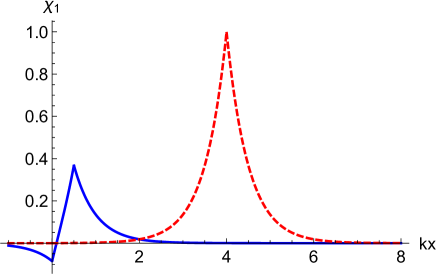
Figure 1: $\chi_{1}(x)$ vs $kx$ with $ka=.5$ (solid) and $ka=4$ (dashed). $B_{1}/2kq$ has been set to 1. Note how the $\chi_{1}$ condensate appears at the position of the $\varphi$ kink ($x=a$).

We have not included the “zero mode” solution Goldstone75 ,Jackiw77 $\chi_{1}^{(0)}(x)\propto\chi_{0}^{\prime}(x)\sim$ sech${}^{2}kx$ of the homogeneous (i.e., sourceless) DE, as this zero mode does not arise in response to the $\chi-\varphi$ interaction, and the solution of interest here, and points forward, is that of (32), which does arise from the two-kink interaction.

The $\boldsymbol{\varphi}_{1}$ correction:  Now denote $\varphi_{1}$ by $\varphi_{1}(x)=\psi(x)$, and again $k_{\chi}=k$, $k_{\varphi}=q$, $x_{\chi}=0$, and $x_{\varphi}=a$. The location of the $\chi$ kink is $x=0$, and that of the $\varphi$ kink is $x=a$, as before. Also define the constant $B_{2}=\beta\eta^{2}\sigma$. Using the same approximations as before, we divide the $x$ space into three regions with functions $\psi_{1}(x)$, $\psi_{2}(x)$, and $\psi_{3}(x)$ in regions I, II, and III, respectively. With the delta function approximation, (23b) is written as

$$\psi^{\prime\prime}(x)-4q^{2}\psi(x)+12q\delta(x-a)\psi(x)=-\frac{2B_{2}}{k}\tanh q(x-a)\delta(x)$$ (33)

with boundary conditions $\psi\rightarrow 0$ as $x\rightarrow\pm\infty$. Each region is again $\delta$ function-free, and the solutions are again of exponential form $e^{\pm 2qx}$. Specifically,

$$\begin{array}[]{ll}\text{I:\ \ \ }\psi_{1}=Ae^{2qx},&x<0\\ \text{II: \ }\psi_{2}=Be^{2qx}+Ce^{-2qx},&0<x<a\\ \text{III: }\psi_{3}=De^{-2qx},&x>a\end{array}$$ (34)

where the coefficients $A,B,C,D$ are now new ones for the $\varphi_{1}$ function. We use continuity of $\psi(x)$ at $x=0$ and $x=a,$ and integrate the DE (33) to obtain constraints on $\psi^{\prime}(0)$ and $\psi^{\prime}(a)$. The coefficients can be determined (see Appendix B) and the resulting solution is given by (see FIG. 2)

$$\varphi_{1}(x)\approx-\frac{\beta\eta}{\sqrt{\lambda_{\chi}\lambda_{\varphi}}}\tanh qa\times\left\{\begin{array}[]{ll}\left(1-\frac{3}{2}e^{-4qa}\right)e^{2qx},&x<0\\ -\frac{3}{2}e^{-4qa}e^{2qx}+e^{-2qx},&0<x<a\\ -\frac{1}{2}e^{-2qx},&x>a\end{array}\right\}$$ (35)

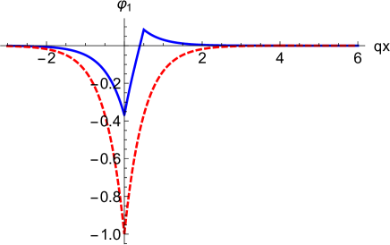
Figure 2: $\varphi_{1}(x)$ vs $qx$ for $qa=.5$ (solid) and $qa=4$ (dashed). $B_{2}/2kq$ has been set to 1. Note how the $\varphi_{1}$ condensate appears at the position of the $\chi$ kink ($x=0$).

Once again, there is a zero mode solution Goldstone75 ,Jackiw77 , $\varphi_{1}^{(0)}(x)\propto\varphi_{0}^{\prime}(x)\sim$ sech${}^{2}q(x-a)$ which solves the homogeneous (sourceless) DE of (23b), but since it has nothing to do with the $\chi-\varphi$ interaction we dismiss it from further consideration.

Note that for $a\neq 0$ (32) and (35) suggest that the correction for each kink/wall solution manifests itself in the form of a “ghostly” displaced scalar condensate, residing within the other kink/wall. For example, the $\chi_{1}$ correction is pronounced near $x=a$ (the location of the $\varphi$ kink), and the $\varphi_{1}$ correction is pronounced near $x=0$ (the location of the $\chi$ kink). (From (23) it is seen that a correction $\psi_{1}(x)$ for either kink can not vanish at the location of the other kink, as the source term for each correction maximizes at the location of the other kink.) Therefore, the $\chi$ kink has a topological structure from the $\chi$ field, along with a condensate from the $\varphi$ field, and vice versa. The kink, along with the condensate within it, might be referred to as a “structured” kink. The condensates described by $\chi_{1}$ and $\varphi_{1}$ vanish for $a=0$, i.e., when the centers of the kinks coincide. Therefore, within either kink/wall there appears a small additional energy density due to the condensate when there is a nonzero separation between them ($a\neq 0$). However, this extra mass disappears when the two kinks overlap, suggesting the existence of a weakly bound state under certain circumstances.

VII Structured solitons

VII.1 Displaced condensates

The $\chi_{0}(x)$ and $\varphi_{0}(x)$ static kinks are located at $x=0$ and $x=a$, respectively. The excitation modes $\chi_{1}(x)$ and $\varphi_{1}(x)$ are described by (32) and (35), and each exhibits an enhancement, or scalar field condensate, at the position of the other kink. Specifically, the $\chi_{1}$ mode is concentrated at $x=a$, the location of the $\varphi_{0}$ kink, and the $\varphi_{1}$ mode is concentrated at at $x=0$, the location of the $\chi_{0}$ kink. The “widths” of the condensates are comparable to, or on the order of, those of the host kinks.

These condensate modes are nontopological in nature, as each mode solution rapidly approaches its asymptotic value of zero. However, a condensate has an attendant “mass” (surface energy, for a domain wall) that we can denote by $\Sigma$. This mass is obtained from the energy-momentum tensor $T_{\mu\nu}^{\psi}$ associated with the condensate; specifically, $\Sigma_{\psi}=\int T_{00}^{\psi}(x)dx$ for each condensate mode ($\psi=\chi$ or $\varphi$). We consider the kinks to be separated by a distance $a$, and assume, for simplicity, that $\chi_{0}\approx\eta$ at the location of $\varphi_{0}$ (i.e., at $x\sim a>0$) and $\varphi_{0}\approx-\sigma$ at the location of $\chi_{0}$ (i.e., at $x\sim 0$). The kink separation is considered to be on the order of, or greater than, the kink “widths”, $a\gtrsim w_{\chi},w_{\varphi}$, although with some justification we will be able to extrapolate our results for the case where $a\rightarrow 0$.

VII.2 “Masses” of the condensates

The basic idea used here is to isolate the contribution of each condensate ($\psi_{1}(x)$) to the energy-momentum $T_{\mu\nu}^{\psi}(x)$ and then integrate $T_{00}^{\psi}(x)$ to obtain the mass $\Sigma_{\psi}(a)=\int T_{00}^{\psi}(x)dx$ which will depend upon the separation distance $a$ between the $\chi_{0}$ and $\varphi_{0}$ kinks. The computational details are given in Appendix C, and we simply state the results here for $\Sigma_{\chi}$ and $\Sigma_{\varphi}$, i.e., the masses of the $\chi_{1}$ and $\varphi_{1}$ condensates, respectively:

$$\Sigma_{\chi}(a) \approx 2\beta^{2}\eta\sigma^{2}\left[\sqrt{\frac{\lambda_{\chi}}{2}}\frac{\tanh^{2}ka}{\lambda_{\chi}\lambda_{\varphi}}+\sqrt{\frac{2}{\lambda_{\varphi}}}\frac{\tanh ka}{\sqrt{\lambda_{\chi}\lambda_{\varphi}}}\right]$$ (36a)

$$\Sigma_{\varphi}(a) \approx 2\beta^{2}\eta^{2}\sigma\left[\sqrt{\frac{\lambda_{\varphi}}{2}}\frac{\tanh^{2}qa}{\lambda_{\chi}\lambda_{\varphi}}+\sqrt{\frac{2}{\lambda_{\chi}}}\frac{\tanh qa}{\sqrt{\lambda_{\chi}\lambda_{\varphi}}}\right]$$ (36b)

The results for the “masses” $\Sigma_{\chi}$ and $\Sigma_{\varphi}$, given by (36) allow us to reasonably expect that each mass decreases with decreasing separation distance $a$, presumably to zero when the centers of the two kinks coincide. (This expectation is strengthened by noticing that the corrections $\chi_{1}$ and $\varphi_{1}$ vanish as $a\rightarrow 0$.) Such a decrease in the total system mass suggests the presence of a weak ($\propto\beta^{2}$), but nonzero, force of attraction between the two kinks, allowing a weakly bound state to exist. This attractive force must be of fairly short range, since $\tanh\kappa a$ approaches unity for $\kappa a\sim 2$, where $\kappa=1/w$ is the inverse width parameter ($\kappa=k=1/w_{\chi}$ or $\kappa=q=1/w_{\varphi}$).

VII.3 Weakly bound states

A structured $\chi$ soliton resides at $x=0$, comprised of the $\chi_{0}$ topological kink and the $\varphi_{1}$ condensate. Likewise, a structured $\varphi$ soliton resides at $x=a$, comprised of the $\varphi_{0}$ topological kink and the $\chi_{1}$ condensate. Each topological kink has an energy density of the form $T_{00}^{\psi_{0}}(x)=\frac{1}{2}\lambda v^{4}$sech${}^{4}\kappa x$, where $v=\eta$ or $\sigma$, $\lambda=\lambda_{\chi}$ or $\lambda_{\varphi}$, and $\kappa=k$ or $q$. The “masses” of the topological kinks are

$$M_{\chi}=\frac{2}{3}\sqrt{2\lambda_{\chi}}\eta^{3},\ \ \ \ \ M_{\varphi}=\frac{2}{3}\sqrt{2\lambda_{\varphi}}\sigma^{3}$$ (37)

Therefore, the total “masses” of the structured solitons with condensates are

$$\mu_{\chi}(a)=M_{\chi}+\Sigma_{\varphi}(a),\ \ \ \ \ \mu_{\varphi}(a)=M_{\varphi}+\Sigma_{\chi}(a)$$ (38)

with $\Sigma_{\chi}$ and $\Sigma_{\varphi}$ given by (36). (The “masses” $\mu_{\chi}$, $\mu_{\varphi}$ have dimensions of mass for $1+1$ dimensional kinks or mass³ for $3+1$ dimensional domain walls.)

It has been suggested that when the two structured solitons are at the same position, $a\rightarrow 0$, then the condensate masses vanish, $\Sigma_{\chi}\rightarrow 0$ and $\Sigma_{\varphi}\rightarrow 0$. This suggestion is strengthened by noticing from (32) and (35) that $\chi_{1}\rightarrow 0$ and $\varphi_{1}\rightarrow 0$ as $a\rightarrow 0$, without an assumption that $\kappa a\gtrsim 1$. We therefore expect the corresponding energy densities $T_{00}^{\chi,\varphi}$ to vanish as $a\rightarrow 0$, i.e., $\Sigma_{\chi}\rightarrow 0$, $\Sigma_{\varphi}\rightarrow 0$ as $a\rightarrow 0$.  So when the two structured solitons coincide at the same position, the mass of each decreases so that there is a “mass defect” of the two-soliton system

$$\Delta\mu=\mu_{\text{Total,max}}-M_{\text{Total}}=\left(\Sigma_{\chi}+\Sigma_{\varphi}\right)_{\text{max}}$$ (39)

where $\Sigma_{\text{max}}$ is the maximum value of $\Sigma$, evaluated for $\tanh\kappa a=1$ ($\kappa=k$ or $q)$. This mass defect, or binding energy, is the amount of energy required to separate a two-soliton bound state at rest into two separate solitons. We surmise that the structured solitons can form a weakly bound state if the overall force between them is repulsive, since a small dip in the local maximum of the classical potential energy $U(a)$ at $a=0$ produces a small barrier around $a=0$, with $a=0$ being a point of (otherwise) unstable equilibrium, where (excluding the binding energy effect due to $\Delta\mu$), $U(0)=U_{\text{max}}>0$. Thus, a small perturbation with energy $E\geq\Delta\mu$ to the bound state can separate the two kinks at rest. The bound state energy is relatively small since $\Delta\mu\propto\beta^{2}$ and $|\beta|\ll\lambda_{\chi},\lambda_{\varphi}$. The potential energy $U(0)$ of the weakly bound system is then converted into kinetic energy of the kinks. Of course, more strongly bound states may exist for $U(0)<0$.

VIII Classical motion

Interaction energy:  The perturbing potential describing the interaction between the fields $\chi$ and $\varphi$ is given by (2) with $|\beta|\ll\lambda_{\chi}$, $\lambda_{\varphi}$, and we allow $\beta$ to be positive or negative. Since the field corrections $\chi_{1}$ and $\varphi_{1}$ are considered to be very small, with the base functions $\chi_{0}$ and $\varphi_{0}$ dominating, we now neglect the small corrections and approximate $V_{1}(\chi,\varphi)$ by $V_{1}(\chi_{0},\varphi_{0})$. The fields $\chi_{0}$ and $\varphi_{0}$ obey the equations of motion that follow from $\mathcal{L}_{0}(\chi_{0},\varphi_{0})=\frac{1}{2}(\partial\chi_{0})^{2}+\frac{1}{2}(\partial\varphi_{0})^{2}-V_{0}(\chi_{0},\varphi_{0})$ with static solutions given by (18). With our notation $k_{\chi}=k$, $k_{\varphi}=q$, $x_{\chi}=0$, and $x_{\varphi}=a$, these solutions take the form

$$\chi_{0}(x)=\eta\tanh kx,\ \ \ \ \ \varphi_{0}(x)=\sigma\tanh q(x-a)$$ (40)

The energy density (surface energy density for domain walls) associated with the topological kink solutions (40) is $T_{00}^{(0)}=-\mathcal{L}_{0}(\chi_{0},\varphi_{0})$, and the residual energy density $\rho_{1}=-\mathcal{L}_{I}(\chi_{0},\varphi_{0})=V_{1}(\chi_{0},\varphi_{0})$ is that associated with the kink interactions, namely,

$$\rho_{1}=V_{1}(\chi_{0},\varphi_{0})=\frac{1}{2}\beta\left(\chi_{0}^{2}-\eta^{2}\right)\left(\varphi_{0}^{2}-\sigma^{2}\right)=\frac{1}{2}\beta\eta^{2}\sigma^{2}\text{ sech}^{2}kx\cdot\text{sech}^{2}q(x-a)$$ (41)

The “potential energy” of interaction $U(a)$ (potential energy/unit area, for domain walls) is given by the integration of $\rho_{1}(x,a)$,

$$U(a)=\int\rho_{1}(x,a)dx=\frac{1}{2}\beta\eta^{2}\sigma^{2}I(a)=\frac{1}{2}\beta\eta^{2}\sigma^{2}\text{ }\int\text{sech}^{2}kx\cdot\text{sech}^{2}q(x-a)dx$$ (42)

This is viewed as the potential energy of the $\varphi_{0}$ kink in the presence of the $\chi_{0}$ kink note .

The integral $I(a)=\int$sech${}^{2}kx\cdot$sech${}^{2}q(x-a)dx$ can be approximated if we take, for example, $k\gtrsim q$, and use (26), with sech${}^{2}kx\rightarrow\frac{2}{k}\delta(x)$. Integration gives note1 $I(a)\rightarrow\frac{2}{k}$sech${}^{2}qa$. With this approximation we have

$$U(a)=\frac{1}{2}\beta\eta^{2}\sigma^{2}I(a)=\frac{\beta\eta^{2}\sigma^{2}}{k}\ \text{sech}^{2}qa=U_{0}\ \text{sech}^{2}qa,\ \ \ \ \ U_{0}=\frac{\beta\eta^{2}\sigma^{2}}{k}$$ (43)

The sign of the potential energy $U(a)$ is governed by the sign of $\beta$, so that $U\geq 0$ for $\beta>0$ and $U\leq 0$ for $\beta<0$. For $\beta>0$ the position $a=0$ locates a point of unstable equilibrium, while for $\beta<0$ the point $a=0$ is one of stable equilibrium. The maximum magnitude of $U(a)$ is $|U|_{\max}=|\beta|\eta^{2}\sigma^{2}/k$.

Interkink force:  The “force” of interaction $F_{x}(a)$ (force per unit area for domain walls) between the two kinks (e.g., the force on $\varphi_{0}$ at $x=a$ due to $\chi_{0}$ at $x=0$) is

$$F_{x}(a)=-\frac{\partial U(a)}{\partial a}=f_{0}\tanh qa\cdot\text{sech}^{2}qa,\ \ \ \ \ f_{0}=2qU_{0}=2\beta\eta^{2}\sigma^{2}\frac{q}{k}$$ (44)

For $\beta>0$ the force is repulsive and for $\beta<0$ the force is attractive. The magnitude $|F_{x}|$ maximizes at $qa=\frac{1}{2}\ln(2+\sqrt{3})\approx\frac{2}{3}$, corresponding to a separation distance between kink centers of $a\sim\frac{2}{3}w_{\varphi}$, i.e., roughly $2/3\times$ the width of the $\varphi$ kink.

Motion:  The classical motion of the system then depends upon whether the potential $U(a)$ is repulsive $(\beta>0)$ or attractive $(\beta<0)$, and can then be described as a classical two-body system, assuming that when dissipative effects due to scalar radiation of the $\chi$ and $\varphi$ fields are neglected, the mechanical energy $E=T(a)+U(a)$ is conserved, where $T(a)$ is the kinetic energy of the system. Classical turning points of the two kink system depend upon the total energy $E$ and the potential energy $|U_{\text{max}}|=|U_{0}|$.

For a repulsive interaction $(\beta>0)$ turning points can exist for $E<U_{0}$, so that the kinks have a minimum distance of approach. We recall, however, that for the (otherwise) maximum of $U(0)$ there is a small dip at $a=0$ due to the $\psi_{1}(x)$ corrections and the associated mass defect $\Delta\mu$ of (39), which is $O(\beta^{2})$, so that a weakly bound state can exist even for $\beta>0$.

On the other hand, for an attractive interaction $(\beta<0)$ the $\chi$ and $\varphi$ kinks can form a bound state. A conserved topological current density (see, e.g., Rajaraman ,Vach ,Manton ) is $j^{\mu}=\frac{1}{2v}\epsilon^{\mu\nu}\partial_{\nu}\psi$ (with $\psi=\chi$ or $\varphi$, $v=\eta$ or $\sigma$, and $\epsilon^{01}=1$), so that the topological charge is $Q=\frac{1}{v}\int_{-\infty}^{\infty}\partial_{x}\psi dx=\frac{1}{v}[\psi(\infty)-\psi(-\infty)]=+1$ for $\chi$ or $\varphi$ kinks and $Q=-1$ for $\bar{\chi}$ or $\bar{\varphi}$ antikinks. The corresponding charges for $(\chi,\varphi)$ and $(\bar{\chi},\bar{\varphi})$ bound states are $Q=+2$ and $Q=-2$, respectively, and $Q=0$ for $(\bar{\chi},\varphi)$ and $(\chi,\bar{\varphi})$ states. It should also be pointed out that a general system containing many kinks and antikinks will accommodate collisions and annihilations of kinks and antikinks of the same type. The description of motion in this case is much more complicated. (See, for example, Campbell regarding kink-antikink interactions in the $\phi^{4}$ model, and Alonso1 for kink interactions in a two-component model).

IX Meson mixing

The model given by (1) and (2) has a mass (squared) matrix $\boldsymbol{M}^{2}$ given by (4) which is associated with the perturbative “meson” particle “flavor” states $\chi$ and $\varphi$. For $\beta\neq 0$ there are off-diagonal terms due to the interacting scalar fields, indicating that the flavor states are not mass eigenstates. The mass eigenvalues of $\boldsymbol{M}^{2}$ are given by (5). Let us now denote $m_{+}=m_{1}$ and $m_{-}=m_{2}$, with $m_{1}>m_{2}$. Then, in terms of $m_{1,2}$, $(m_{1}>m_{2})$,

$$\begin{array}[]{cc}m_{1}^{2}=\frac{1}{2}\left[m_{\chi}^{2}+m_{\varphi}^{2}+\sqrt{4\mu^{4}+(m_{\chi}^{2}-m_{\varphi}^{2})^{2}}\right]\vskip 3.0pt plus 1.0pt minus 1.0pt&\\ m_{2}^{2}=\frac{1}{2}\left[m_{\chi}^{2}+m_{\varphi}^{2}-\sqrt{4\mu^{4}+(m_{\chi}^{2}-m_{\varphi}^{2})^{2}}\right]&\end{array}$$ (45)

and the corresponding mass eigenstates are $\phi_{+}=\phi_{1}$ and $\phi_{-}=\phi_{2}$, and the flavor states $\chi$ and $\varphi$ are linear combinations of $\phi_{1}$ and $\phi_{2}$, as shown in (6). Now, for the individual noninteracting fields $\chi$ and $\varphi$ there are, in addition to the kink modes, nonperturbative modes including a zero mode $\psi_{0}$ and a discrete excitation mode $\psi_{D}$ for each field, along with the meson radiation modes, labelled here as $\varepsilon_{p}(x,t)$ with momentum $p$. A meson radiation mode has energy $\omega=\sqrt{p^{2}+m_{\psi}^{2}}$ with $m_{\psi}^{2}=m_{\chi}^{2},m_{\varphi}^{2}$ and

$$\varepsilon_{p}(x,t)=f_{p}(x)e^{-i\omega t},\ \ \ \ f_{p}(x)=Ae^{ipx}[3\tanh^{2}z-1-p^{2}w^{2}-iwp\tanh z]$$ (46)

with $z=\kappa(x-x_{0})$, $w=1/\kappa$, with $\kappa=k,q$ and $p$ is the momentum. The asymptotic scattering solutions are given by $f_{p}(x)\propto e^{ipx}$.

Mixing of meson particle states:  We denote the (perturbative) meson particle flavor states at time $t=0$ by $|\chi(0)\rangle=|\chi\rangle,$ $|\varphi(0)\rangle=|\varphi\rangle$, and the mass eigenstates at time $t=0$ are $|\phi_{1}(0)\rangle=|\phi_{1}\rangle,\ |\phi_{2}(0)\rangle=|\phi_{2}\rangle$:

$$\left(\begin{array}[]{c}|\chi\rangle\\ |\varphi\rangle\end{array}\right)=\left(\begin{array}[]{cc}\cos\theta&\sin\theta\\ -\sin\theta&\cos\theta\end{array}\right)\ \left(\begin{array}[]{c}|\phi_{1}\rangle\\ |\phi_{2}\rangle\end{array}\right)=\boldsymbol{R}(\theta)\ \left(\begin{array}[]{c}|\phi_{1}\rangle\\ |\phi_{2}\rangle\end{array}\right)$$ (47)

where $\boldsymbol{R}(\theta)$ is the rotation matrix, $\theta$ is the mixing angle, and the kets $|\phi_{1,2}\rangle$ represent orthonormal states,

$$\langle\phi_{1}|\phi_{1}\rangle=\langle\phi_{2}|\phi_{2}\rangle=1,\ \ \ \ \langle\phi_{1}|\phi_{2}\rangle=0$$ (48)

The energy eigenstates evolve: $|\phi_{i}(t)\rangle=|\phi_{i}(0)\rangle e^{-iE_{i}t}=|\phi_{i}\rangle e^{-iE_{i}t}$, so that

$$\left(\begin{array}[]{c}|\phi_{1}(t)\rangle\\ |\phi_{2}(t)\rangle\end{array}\right)=\left(\begin{array}[]{c}|\phi_{1}\rangle e^{-iE_{1}t}\\ |\phi_{2}\rangle e^{-iE_{2}t}\end{array}\right)=\boldsymbol{R}^{-1}(\theta)\ \left(\begin{array}[]{c}|\chi(t)\rangle\\ |\varphi(t)\rangle\end{array}\right)$$ (49)

and

$$\left(\begin{array}[]{c}|\chi(t)\rangle\\ |\varphi(t)\rangle\end{array}\right)=\boldsymbol{R}(\theta)\left(\begin{array}[]{c}|\phi_{1}\rangle e^{-iE_{1}t}\\ |\phi_{2}\rangle e^{-iE_{2}t}\end{array}\right)=\left(\begin{array}[]{cc}\cos\theta&\sin\theta\\ -\sin\theta&\cos\theta\end{array}\right)\left(\begin{array}[]{c}|\phi_{1}\rangle e^{-iE_{1}t}\\ |\phi_{2}\rangle e^{-iE_{2}t}\end{array}\right)$$ (50)

Therefore,

$$\begin{array}[]{ll}|\chi(t)\rangle&=\cos\theta|\phi_{1}\rangle e^{-iE_{1}t}+\sin\theta|\phi_{2}\rangle e^{-iE_{2}t}\\ |\varphi(t)\rangle&=-\sin\theta|\phi_{1}\rangle e^{-iE_{1}t}+\cos\theta|\phi_{2}\rangle e^{-iE_{2}t}\end{array}$$ (51)

These results can be used to write CMS

$$\begin{array}[]{cc}|\chi(t)\rangle=(e^{-iE_{1}t}\cos^{2}\theta+e^{-iE_{2}t}\sin^{2}\theta)|\chi\rangle+\sin\theta\cos\theta(e^{-iE_{2}t}-e^{-iE_{1}t})|\varphi\rangle&\\ |\varphi(t)\rangle=(e^{-iE_{2}t}-e^{-iE_{1}t})\sin\theta\cos\theta|\chi\rangle+(e^{-iE_{1}t}\sin^{2}\theta+e^{-iE_{2}t}\cos^{2}\theta)|\varphi\rangle&\end{array}$$ (52)

Probabilities:  The probability that a $\chi$ meson emitted at time $t=0$ becomes either a $\chi$ or $\varphi$ meson at time $t$ is CMS ,AC18

$$\begin{array}[]{ll}P(\chi\rightarrow\chi,t)&=|\langle\chi|\chi(t)\rangle|^{2}=(e^{-iE_{1}t}\cos^{2}\theta+e^{-iE_{2}t}\sin^{2}\theta)^{2}\\ &=1-\frac{1}{2}\sin^{2}(2\theta)[1-\cos(E_{1}-E_{2})t]\end{array}$$ (53c)

$$\begin{array}[]{ll}P(\chi\rightarrow\varphi,t)&=|\langle\varphi|\chi(t)\rangle|^{2}=[\sin\theta\cos\theta(e^{-iE_{2}t}-e^{-iE_{1}t})]^{2}\\ &=\frac{1}{2}\sin^{2}(2\theta)[1-\cos(E_{1}-E_{2})t]\end{array}$$ (53f)

High energy limit:  For ultrarelativistic particles with $E\gg m$ and $E\approx E_{1}\approx E_{2}$, write $E_{1}-E_{2}=(E_{1}^{2}-E_{2}^{2})/(E_{1}+E_{2})\approx\frac{(m_{1}^{2}-m_{2}^{2})}{2E}=\frac{\Delta m^{2}}{2E}$, where $\Delta m^{2}=m_{1}^{2}-m_{2}^{2}$. Then for an ultrarelativistic particle with speed $v\approx 1$ emitted from $x=0$ at time $t=0$ we have at a distance $x$ a phase for which $(E_{1}-E_{2})t\approx\frac{\Delta m^{2}}{2E}x=\frac{2\pi x}{L}$, where the oscillation length is $L=4\pi E/\Delta m^{2}$. Therefore, the probability that an ultrarelativistic $\chi$ particle emitted from $x=0$ at time $t=0$ reaches a stationary $\varphi$ kink located at $x=a$ in the form of a $\varphi$ particle at time $t$ is

$$P(\chi\rightarrow\varphi,t\approx a)=\frac{1}{2}\sin^{2}(2\theta)\left[1-\cos\frac{2\pi a}{L}\right]$$ (54)

A beam consisting of $N_{\chi}^{(0)}$ ultrarelativistic monoenergetic $\chi$ particles emitted from $x=0$ reaches the $\varphi$ kink at $x=a$ with only a number of $N_{\chi}(a)\approx N_{\chi}^{(0)}(1-P_{\chi\rightarrow\varphi})$ of $\chi$ particles. The $\varphi$ mesons do not reflect from an unexcited $\varphi$ kink (see, e.g.,Goldstone75 ; Jackiw77 ; Rajaraman ), and therefore do not exert a force upon it. The $\chi$ meson force upon the $\varphi$ kink is thus reduced by a factor of $N_{\chi}^{(0)}P_{\chi\rightarrow\varphi}$, where $P_{\chi\rightarrow\varphi}=P(\chi\rightarrow\varphi,t\approx a)$.

Low energy limit:  For low energy particles with $p_{1}\approx p_{2}\ll m$ and $E\approx m$, the situation is more complicated, in that it is found that different mass eigenstates which reach the same position $x=a$ at the same time are actually emitted from the source at different times Kobach18PLB . This complication will be further compounded if there is a nontrivial spectrum of energies associated with the emitted $\chi$ radiation. No attempt, therefore, is made here to extract any useful quantitative information concerning the actual force exerted on a $\varphi$ kink by emitted $\chi$ bosons.

Meson-kink interactions:  Some qualitative remarks may be made, however, concerning effects of meson-kink interactions. First, if a $\chi$ meson transforms into a $\varphi$ meson when reaching a $\varphi$ kink, these $\varphi$ mesons do not reflect from the $\varphi$ kink, but merely experience a phase shift Goldstone75 ; Jackiw77 ; Rajaraman . Also, high energy $\chi$ particles with wavelength $\lambda\ll w_{\varphi}$, i.e., $p\gg w_{\varphi}^{-1}=q$, have essentially no reflection from the $\varphi$ kink, that is, the reflection coefficient $\mathcal{R}\approx 0$ VSbookSec13 . But for very low energy particles with $\lambda\gg w_{\varphi}$, or $p\ll w_{\varphi}^{-1}=q$, the reflection is strong with $\mathcal{R}\approx 1$ VSbookSec13 , so that most very low energy $\chi$ particles are reflected and can therefore produce a scalar radiation force on the $\varphi$ kink. This force will vary with the probability $P_{\chi\rightarrow\varphi}$, which, in turn, will depend upon the position $a$ of the $\varphi$ kink.

X Summary

A Rayleigh-Schrödinger perturbation scheme has been developed in order to study the interactions of kinks or domain walls formed from two different scalar fields $\chi$ and $\varphi$. This scheme results in successive sets of corrections to the zero order solitonic solutions $\chi_{0}(x)$ and $\varphi_{0}(x)$ satisfying an unperturbed system with potential $V_{0}(\chi,\varphi)$. The perturbation is introduced through an interaction potential $V_{1}(\chi,\varphi)$. The particular model studied here uses the quartic potential $V_{0}=\frac{1}{4}\lambda_{\chi}(\chi^{2}-\eta^{2})^{2}+\frac{1}{4}\lambda_{\varphi}(\varphi^{2}-\sigma^{2})^{2}$ and an interaction potential $V_{1}=\frac{1}{2}\beta(\chi^{2}-\eta^{2})(\varphi^{2}-\sigma^{2})$. The unperturbed static solutions $\chi_{0}(x)$ and $\varphi_{0}(x)$ are represented by the usual $Z_{2}$ kinks. The first order corrections $\chi_{1}(x)$ and $\varphi_{1}(x)$ are found, which exhibit the peculiar property that the interaction induces each kink to form a condensate within the other kink. Therefore the $\chi$ kink acquires a $\varphi$ condensate, and the $\varphi$ kink acquires a $\chi$ condensate.

The masses of these condensates are determined, and it is reasoned that the condensate masses decrease with separation distance between the kinks, and vanishes when the kinks coincide. The associated mass defect implies the possible existence of a weakly bound state when the overall interkink force is repulsive. When subjected to a small disturbance, the weakly bound two-kink state can fission into two separate kinks with kinetic energies.

A classical potential energy of the system and an interkink force are defined, allowing a qualitative description of the classical motion of the system. The interkink force can be either attractive or repulsive, depending upon the sign of the coupling control parameter $\beta$. The system can therefore accommodate scattering states and bound states. In the case of an attractive interaction force, the bound states can be much more tightly bound than the weakly bound states associated with a repulsive potential, with the composite two-kink bound state having topological charge of $Q=\pm 2$ or $0$.

Finally, it is pointed out that an interaction between the $\chi$ and $\varphi$ scalar fields generally results in a nondiagonal mass matrix, indicating that the $\chi$ and $\varphi$ “flavor” states are actually linear combinations of mass eigenstates $\phi_{1}$ and $\phi_{2}$ of the fields. As a consequence, there are oscillations of the flavor states as the mesons from the position $x=0$ of the $\chi$ kink propagate to the position $x=a$ of the $\varphi$ kink. Time-dependent probabilities $P(\chi\rightarrow\chi,t)$ and $P(\chi\rightarrow\varphi,t)$ are found for a $\chi$ boson to be found as a $\chi$ or a $\varphi$ boson at time $t$. For ultrarelativistic particles a standard result is given for the probabilities and oscillation lengths. However, the situation is much murkier for the case of nonrelativistic particles. At any rate, the $\chi$ radiation force exerted upon the $\varphi$ kink will be reduced by an amount that depends upon the meson mixing probabilities.

Appendix A Perturbation expansion scheme

As written in (12)-(14), we can expand $\psi(x,g)$ in powers of $g$, and expand $H(\psi)$ about the unperturbed (base) solution $\psi_{0}$:

$$\begin{array}[]{ll}\psi(x,g)&=\psi_{0}(x)+\delta\psi(x,g)\\ \delta\psi(x,g)&=\sum_{n=1}^{\infty}g^{n}\psi_{n}(x)=g\psi_{1}(x)+g^{2}\psi_{2}(x)+\cdot\cdot\cdot\end{array}$$ (55)

with $\psi=\chi,\varphi$, and

$$H(\chi,\varphi)=H(\psi_{0})+\left(\delta\chi\partial_{\chi}+\delta\varphi\partial_{\varphi}\right)H(\chi,\varphi)\Big{|}_{\chi_{0},\varphi_{0}}+\frac{1}{2}\left(\delta\chi\partial_{\chi}+\delta\varphi\partial_{\varphi}\right)^{2}H(\chi,\varphi)\Big{|}_{\chi_{0},\varphi_{0}}+\cdot\cdot\cdot$$ (56)

where $H=F,G$, and $(\delta\psi\partial_{\psi})^{2}H=(\delta\psi)^{2}\partial_{\psi}^{2}H$ and so on. Since $H=H_{0}+gH_{1}$ this becomes

$$H(\chi,\varphi) =H_{0}(\psi_{0})+\left(\delta\chi\partial_{\chi}+\delta\varphi\partial_{\varphi}\right)H_{0}(\chi,\varphi)\Big{|}_{\chi_{0},\varphi_{0}}+\frac{1}{2}\left(\delta\chi\partial_{\chi}+\delta\varphi\partial_{\varphi}\right)^{2}H_{0}(\chi,\varphi)\Big{|}_{\chi_{0},\varphi_{0}}+\cdot\cdot\cdot$$

$$+gH_{1}(\psi_{0})+g\left(\delta\chi\partial_{\chi}+\delta\varphi\partial_{\varphi}\right)H_{1}(\chi,\varphi)\Big{|}_{\chi_{0},\varphi_{0}}+\frac{1}{2}g\left(\delta\chi\partial_{\chi}+\delta\varphi\partial_{\varphi}\right)^{2}H_{1}(\chi,\varphi)\Big{|}_{\chi_{0},\varphi_{0}}+\cdot\cdot\cdot$$ (57)

The equations of motion for the full system (3) can now be written in expanded form  with the aid of (55)-(57):

$$\begin{array}[]{ll}\square(\chi_{0}+g\chi_{1}+g^{2}\chi_{2}+g^{3}\chi_{3}+\cdot\cdot\cdot)+F_{0}(\chi_{0},\varphi_{0})+gF_{1}(\chi_{0},\varphi_{0})&\\ +\left[\left(g\chi_{1}+g^{2}\chi_{2}+g^{3}\chi_{3}+\cdot\cdot\cdot\right)\partial_{\chi}F_{0}(\chi_{0},\varphi_{0})\right]+\left[\left(g\varphi_{1}+g^{2}\varphi_{2}+g^{3}\varphi_{3}+\cdot\cdot\cdot\right)\partial_{\varphi}F_{0}(\chi_{0},\varphi_{0})\right]&\\ +\frac{1}{2}\left[\left(g\chi_{1}+g^{2}\chi_{2}+\cdot\cdot\cdot\right)^{2}\partial_{\chi}^{2}F_{0}(\chi_{0},\varphi_{0})+\left(g\varphi_{1}+g^{2}\varphi_{2}+\cdot\cdot\cdot\right)^{2}\partial_{\varphi}^{2}F_{0}(\chi_{0},\varphi_{0})\right]&\\ +\left[\left(g\chi_{1}+g^{2}\chi_{2}+\cdot\cdot\cdot\right)\left(g\varphi_{1}+g^{2}\varphi_{2}+\cdot\cdot\cdot\right)\partial_{\chi}\partial_{\varphi}F_{0}(\chi_{0},\varphi_{0})\right]&\\ +g\left[\left(g\chi_{1}+g^{2}\chi_{2}+g^{3}\chi_{3}+\cdot\cdot\cdot\right)\partial_{\chi}F_{1}(\chi_{0},\varphi_{0})\right]+g\left[\left(g\varphi_{1}+g^{2}\varphi_{2}+g^{3}\varphi_{3}+\cdot\cdot\cdot\right)\partial_{\varphi}F_{1}(\chi_{0},\varphi_{0})\right]&\\ +\frac{1}{2}g\left[\left(g\chi_{1}+g^{2}\chi_{2}+\cdot\cdot\cdot\right)^{2}\partial_{\chi}^{2}F_{1}(\chi_{0},\varphi_{0})+\left(g\varphi_{1}+g^{2}\varphi_{2}+\cdot\cdot\cdot\right)^{2}\partial_{\varphi}^{2}F_{1}(\chi_{0},\varphi_{0})\right]&\\ +g\left[\left(g\chi_{1}+g^{2}\chi_{2}+\cdot\cdot\cdot\right)\left(g\varphi_{1}+g^{2}\varphi_{2}+\cdot\cdot\cdot\right)\partial_{\chi}\partial_{\varphi}F_{1}(\chi_{0},\varphi_{0})\right]=0&\end{array}$$ (58)

and similarly for the $\varphi$ equation of motion with $\square\chi\rightarrow\square\varphi$ and $F(\chi,\varphi)\rightarrow G(\chi,\varphi)$. The various $g^{n}$ terms can be collected to give the equations for the $\chi_{n}$ and $\varphi_{n}$.

$$\begin{array}[]{ll}g^{0}:&\square\chi_{0}+F_{0}(\chi_{0},\varphi_{0})=0\\ g^{1}:&\square\chi_{1}+(\chi_{1}\partial_{\chi}+\varphi_{1}\partial_{\varphi})F_{0}(\chi_{0},\varphi_{0})+F_{1}(\chi_{0},\varphi_{0})=0\\ g^{2}:&\square\chi_{2}+\left(\chi_{2}\partial_{\chi}+\varphi_{2}\partial_{\varphi}\right)F_{0}(\chi_{0},\varphi_{0})+\frac{1}{2}\left(\chi_{1}^{2}\partial_{\chi}^{2}+\varphi_{1}^{2}\partial_{\varphi}^{2}\right)F_{0}(\chi_{0},\varphi_{0})\\ &+\chi_{1}\varphi_{1}\partial_{\chi}\partial_{\varphi}F_{0}(\chi_{0},\varphi_{0})+\left(\chi_{1}\partial_{\chi}+\varphi_{1}\partial_{\varphi}\right)F_{1}(\chi_{0},\varphi_{0})=0\end{array}$$ (59)

$$\begin{array}[]{ll}g^{0}:&\square\varphi_{0}+G_{0}(\chi_{0},\varphi_{0})=0\\ g^{1}:&\square\varphi_{1}+(\chi_{1}\partial_{\chi}+\varphi_{1}\partial_{\varphi})G_{0}(\chi_{0},\varphi_{0})+G_{1}(\chi_{0},\varphi_{0})=0\\ g^{2}:&\square\varphi_{2}+\left(\chi_{2}\partial_{\chi}+\varphi_{2}\partial_{\varphi}\right)G_{0}(\chi_{0},\varphi_{0})+\frac{1}{2}\left(\chi_{1}^{2}\partial_{\chi}^{2}+\varphi_{1}^{2}\partial_{\varphi}^{2}\right)G_{0}(\chi_{0},\varphi_{0})\\ &+\chi_{1}\varphi_{1}\partial_{\chi}\partial_{\varphi}G_{0}(\chi_{0},\varphi_{0})+\left(\chi_{1}\partial_{\chi}+\varphi_{1}\partial_{\varphi}\right)G_{1}(\chi_{0},\varphi_{0})=0\end{array}$$ (60)

For our model given by (1) and (2), the first order equations for $\psi_{1}(x)$ are given by (15), with $H_{0}(\chi,\varphi)$ and $H_{1}(\chi,\varphi)$ given by (16).

Appendix B Approximate first order corrections

Solution for $\boldsymbol{\chi}_{1}$:  We have the approximate second order nonhomogeneous differential equation (DE)

$$\psi^{\prime\prime}(x)-4k^{2}\psi(x)+12k\delta(x)\psi(x)=-\frac{2B_{1}}{q}\tanh kx\cdot\delta(x-a)$$ (61)

with the solutions

$$\begin{array}[]{ll}\text{I:\ \ \ }\psi_{1}=Ae^{2kx},&x<0\\ \text{II: \ }\psi_{2}=Be^{2kx}+Ce^{-2kx},&0<x<a\\ \text{III: }\psi_{3}=De^{-2kx},&x>a\end{array}$$ (62)

The continuity of $\psi$ at $x=0$ and $x=a$ gives the following constraints:

$$\begin{array}[]{ll}\psi_{1}(0)=\psi_{2}(0):&A=B+C\\ \psi_{2}(a)=\psi_{3}(a):&Be^{2ka}+Ce^{-2ka}=De^{-2ka}\end{array}$$ (63)

Now upon integrating the DE (61) about $x=\pm\epsilon$ (where the right hand side is absent) and about $x=a\pm\epsilon$ (where the $12k\delta(x)$ term is absent) and taking the limit $\epsilon\rightarrow 0$, we obtain

$$\begin{array}[]{ll}x\approx 0:&\int_{-\epsilon}^{\epsilon}\psi^{\prime\prime}(x)dx-4k^{2}\int_{-\epsilon}^{\epsilon}\psi(x)dx+12k\int_{-\epsilon}^{\epsilon}\psi(x)\delta(x)dx=0\\ x\approx a:&\int_{a-\epsilon}^{a+\epsilon}\psi^{\prime\prime}(x)dx-4k^{2}\int_{a-\epsilon}^{a+\epsilon}\psi(x)dx=-\frac{2B_{1}}{q}\int_{a-\epsilon}^{a+\epsilon}\tanh kx\delta(x-a)dx\end{array}$$ (64)

Keeping in mind that $\psi(x)$ is continuous, so that as $\epsilon\rightarrow 0$, $\int_{-\epsilon}^{\epsilon}\psi(x)dx=0$ and $\int_{a-\epsilon}^{a+\epsilon}\psi(x)dx=0$, we have

$$\begin{array}[]{ll}\psi_{2}^{\prime}(0)-\psi_{1}^{\prime}(0)+12k\psi_{1}(0)=0&\implies B-C+5A=0\\ \psi_{3}^{\prime}(a)-\psi_{2}^{\prime}(a)=-\frac{2B_{1}}{q}\tanh ka&\implies De^{-2ka}+Be^{2ka}-Ce^{-2ka}=\frac{B_{1}}{kq}\tanh ka\end{array}$$ (65)

The four constraint equations given by (63) and (65) allow us to determine

$$A=-\frac{1}{2}B,\ \ \ C=-\frac{3}{2}B,\ \ \ D=\left(e^{4ka}-\frac{3}{2}\right)B,\ \ \ B=\frac{B_{1}}{2kq}e^{-2ka}\tanh ka$$ (66)

From (18) we have $k_{\chi}=k=\sqrt{\lambda_{\chi}/2}\cdot\eta$ and $k_{\varphi}=q=\sqrt{\lambda_{\varphi}/2}\cdot\sigma$. This in conjunction with $B_{1}=\beta\eta\sigma^{2}$ allows us to write the coefficient $B$ as

$$B=\frac{B_{1}}{2kq}e^{-2ka}\tanh ka=\frac{\beta\eta\sigma^{2}}{\sqrt{\lambda_{\chi}\lambda_{\varphi}}\eta\sigma}e^{-2ka}\tanh ka=\frac{\beta\sigma}{\sqrt{\lambda_{\chi}\lambda_{\varphi}}}e^{-2ka}\tanh ka$$ (67)

Then (62), (66), and (67) give us

$$\chi_{1}(x)\approx\frac{\beta\sigma}{\sqrt{\lambda_{\chi}\lambda_{\varphi}}}e^{-2ka}\tanh ka\times\left\{\begin{array}[]{ll}-\frac{1}{2}e^{2kx},&x<0\\ e^{2kx}-\frac{3}{2}e^{-2kx},&0<x<a\\ \left(e^{4ka}-\frac{3}{2}\right)e^{-2kx},&x>a\end{array}\right\}$$ (68)

The correction $|\chi_{1}|$ maximizes at $x=a$, the location of the $\varphi$ kink (FIG. 1). For $x=a$ the correction is, approximately,

$$\chi_{1}(a)\approx\frac{\beta\sigma\tanh ka}{\sqrt{\lambda_{\chi}\lambda_{\varphi}}}(1-\tfrac{3}{2}e^{-4ka})\sim\frac{\beta\sigma}{\sqrt{\lambda_{\chi}\lambda_{\varphi}}}$$ (69)

for $ka\gtrsim 1$ ($a\gtrsim w_{\chi}$). The requirement that $|\chi_{1}(a)|$ is dominated by $|\chi_{0}(a)|\sim\eta$ for $ka\gtrsim 1$, i.e., $|\chi_{1}|/\eta\ll 1$, then translates into the requirement $\left(|\beta|/\sqrt{\lambda_{\chi}\lambda_{\varphi}}\right)\sigma/\eta\ll 1$. For $\sigma/\eta\sim O(1)$ this means that the approximate solution is valid provided that

$$\frac{|\beta|}{\sqrt{\lambda_{\chi}\lambda_{\varphi}}}\frac{\sigma}{\eta}\sim\frac{|\beta|}{\sqrt{\lambda_{\chi}\lambda_{\varphi}}}\ll 1,\ \ \ \text{for}\ \frac{\sigma}{\eta}\sim O(1)$$ (70)

which is in accord with the original assumption that $|\beta|\ll\lambda_{\chi}$, $\lambda_{\varphi}$, so that the perturbing potential $V_{1}$ is a small perturbation to the unperturbed potential $V_{0}$.

Solution for $\boldsymbol{\varphi}_{1}$:  Now denote $\varphi_{1}$ by $\varphi_{1}(x)=\psi(x)$, and again $k_{\chi}=k$, $k_{\varphi}=q$, $x_{\chi}=0$, and $x_{\varphi}=a$. The location of the $\chi$ kink is $x=0$, and that of the $\varphi$ kink is $x=a$, as before. Also define the constant $B_{2}=\beta\eta^{2}\sigma$. Using the same approximations as before, we divide the $x$ space into three regions with functions $\psi_{1}(x)$, $\psi_{2}(x)$, and $\psi_{3}(x)$ in regions I, II, and III, respectively. With the delta function approximation, (23b) is written as

$$\psi^{\prime\prime}(x)-4q^{2}\psi(x)+12q\delta(x-a)\psi(x)=-\frac{2B_{2}}{k}\tanh q(x-a)\delta(x)$$ (71)

with boundary conditions $\psi\rightarrow 0$ as $x\rightarrow\pm\infty$. Each region is again $\delta$ function-free, and the solutions are again of exponential form $e^{\pm 2qx}$. Specifically,

$$\begin{array}[]{ll}\text{I:\ \ \ }\psi_{1}=Ae^{2qx},&x<0\\ \text{II: \ }\psi_{2}=Be^{2qx}+Ce^{-2qx},&0<x<a\\ \text{III: }\psi_{3}=De^{-2qx},&x>a\end{array}$$ (72)

where the coefficients $A,B,C,D$ are now new ones for the $\varphi_{1}$ function. We use continuity of $\psi(x)$ at $x=0$ and $x=a,$ and integrate the DE (71) to obtain constraints on $\psi^{\prime}(0)$ and $\psi^{\prime}(a)$.

The continuity of $\psi$ at $x=0$ and $x=a$ gives the following constraints:

$$\begin{array}[]{ll}\psi_{1}(0)=\psi_{2}(0):&A=B+C\\ \psi_{2}(a)=\psi_{3}(a):&Be^{2qa}+Ce^{-2qa}=De^{-2qa}\end{array}$$ (73)

Integration of the DE (71) about $x=\pm\epsilon$ and about $x=a\pm\epsilon$ and taking the limit $\epsilon\rightarrow 0$, we obtain

$$\begin{array}[]{ll}\psi_{2}^{\prime}(0)-\psi_{1}^{\prime}(0)=\frac{2B_{2}}{k}\tanh qa&\implies B-C-A=\frac{B_{2}}{kq}\tanh qa\\ \psi_{3}^{\prime}(a)-\psi_{2}^{\prime}(a)+12q\psi_{3}(a)=0&\implies 5De^{-2qa}=Be^{2qa}-Ce^{-2qa}\end{array}$$ (74)

The constraint equations given by (73) and (74) yield

$$A=\left(1-\frac{3}{2}e^{-4qa}\right)C,\ \ \ B=-\frac{3}{2}Ce^{-4qa},\ \ \ D=-\frac{1}{2}C,\ \ \ C=-\frac{B_{2}}{2kq}\tanh qa$$ (75)

Using $k=\sqrt{\lambda_{\chi}/2}\cdot\eta$ and $q=\sqrt{\lambda_{\varphi}/2}\cdot\sigma$, along with $B_{2}=\beta\eta^{2}\sigma$ allows us to write the coefficient $C$ as

$$C=-\frac{B_{2}}{2kq}\tanh qa=-\frac{\beta\eta^{2}\sigma}{\sqrt{\lambda_{\chi}\lambda_{\varphi}}\eta\sigma}\tanh qa=-\frac{\beta\eta}{\sqrt{\lambda_{\chi}\lambda_{\varphi}}}\tanh qa$$ (76)

Then (72), (75), and (76) give

$$\varphi_{1}(x)\approx-\frac{\beta\eta}{\sqrt{\lambda_{\chi}\lambda_{\varphi}}}\tanh qa\times\left\{\begin{array}[]{ll}\left(1-\frac{3}{2}e^{-4qa}\right)e^{2qx},&x<0\\ -\frac{3}{2}e^{-4qa}e^{2qx}+e^{-2qx},&0<x<a\\ -\frac{1}{2}e^{-2qx},&x>a\end{array}\right\}$$ (77)

The correction $|\varphi_{1}|$ maximizes at $x=0$, the location of the $\chi$ kink (FIG. 2). The assumption that $|\varphi_{1}|\ll\sigma$ is satisfied if $(|\beta|/\sqrt{\lambda_{\chi}\lambda_{\varphi}})\eta/\sigma\ll 1$. So the approximate solution for $\varphi_{1}$ is valid provided that

$$\frac{|\beta|}{\sqrt{\lambda_{\chi}\lambda_{\varphi}}}\frac{\eta}{\sigma}\sim\frac{|\beta|}{\sqrt{\lambda_{\chi}\lambda_{\varphi}}}\ll 1,\ \ \ \text{for}\ \frac{\eta}{\sigma}\sim O(1)$$ (78)

Therefore (70) and (78) imply that the approximate solutions for $\chi_{1}$ and $\varphi_{1}$ are valid if $|\beta|\ll\sqrt{\lambda_{\chi}\lambda_{\varphi}}$ and $\sigma\sim\eta$, which again is in accord with the original assumption that $|\beta|\ll\lambda_{\chi}$, $\lambda_{\varphi}$, so that the perturbing potential $V_{1}$ is a small perturbation to the unperturbed potential $V_{0}$.

Once again, the particular solution of (77) is accompanied by the zero mode solution $\varphi_{1}^{(0)}(x)\propto\varphi_{0}^{\prime}(x)\sim$ sech${}^{2}q(x-a)$ which solves the homogeneous (sourceless) DE of (23b), but since it has nothing to do with the $\chi-\varphi$ interaction we dismiss it from further consideration.

Appendix C Condensate masses

“Mass” of the $\boldsymbol{\chi}_{1}$ condensate:  The energy-momentum tensor for the $\chi$ field is

$$T_{\mu\nu}^{\chi}=\partial_{\mu}\chi\partial_{\nu}\chi-\eta_{\mu\nu}\mathcal{L}_{\chi}$$ (79)

where $\mathcal{L}_{\chi}=\mathcal{L}_{\chi}^{(0)}+\mathcal{L}_{I}$,

$$\mathcal{L}_{\chi}^{(0)}=\frac{1}{2}(\partial\chi)^{2}-\frac{1}{4}\lambda_{\chi}(\chi^{2}-\eta^{2})^{2},\ \ \ \ \ \mathcal{L}_{I}=-V_{1}=-\frac{1}{2}\beta(\chi^{2}-\eta^{2})(\varphi^{2}-\sigma^{2})$$ (80)

The idea is to calculate the energy-momentum $T_{\mu\nu}^{\chi}$ that arises from the interaction of the $\chi$ and $\varphi$ kinks. This means that we dismiss any contributions that arise from the pure zero modes $\chi_{1}^{(0)}(x)$ and $\varphi_{1}^{(0)}(x)$, as these modes are solutions of the homogeneous (i.e., sourceless) DEs for $\chi_{1}$ and $\varphi_{1}$, and therefore do not arise from the $\chi-\varphi$ interaction.

For the region near the $\varphi_{0}$ kink, $x=a$, we take $\chi(x\sim a)\approx\eta+\chi_{1}(x)$. (We can also note from (35) that near $x\sim a$ there is a tiny peak in $\varphi_{1}$ with $\varphi_{1}(x\sim a)\propto\beta\eta e^{-2qa}$ which we neglect for $qa\gtrsim 1,$ so that $\varphi_{1}(x\sim a)\approx 0$.) Keeping in mind that $|\chi_{1}|\ll\eta$ and retaining dominant terms results in

$$T_{00}^{\chi}(x\sim a)=-\mathcal{L}_{\chi}(x\sim a)\approx\frac{1}{2}(\chi_{1}^{\prime})^{2}+\lambda_{\chi}\eta^{2}\chi_{1}^{2}+\beta\eta\sigma^{2}\chi_{1}\text{ sech}^{2}q(x-a)$$ (81)

where ${}^{\prime}=\partial_{x}=\partial/\partial x$. This $T_{00}^{\chi}(x\sim a)$ is then the energy density associated with the $\chi_{1}$ field, which is concentrated near $x=a$. An integration of this energy density then gives the mass $\Sigma_{\chi}$ of the $\chi_{1}$ condensate. Referring back to (32) for the solution of $\chi_{1}$, we note that for $ka\gtrsim 1$ (or $a\gtrsim w_{\chi}$), that $e^{-2ka}e^{2kx}\ll 1$ for $x<0$, and the solution for $x<0$ can be ignored. Furthermore, for $ka\gtrsim 1$ and $x\sim a$ we have $e^{-2kx}\ll e^{2kx}$ and $e^{4ka}\gg\frac{3}{2}$ so that (32) simplifies to

$$\chi_{1}(x\sim a)\approx B_{0}e^{-2ka}\times\left\{\begin{array}[]{ll}e^{2kx},&x<a\\ e^{4ka}e^{-2kx},&x>a\end{array}\right\}$$ (82)

where

$$B_{0}=\frac{\beta\sigma}{\sqrt{\lambda_{\chi}\lambda_{\varphi}}}\tanh ka$$ (83)

Using (82) and (83) to evaluate (81) for $x\sim a$ leads to

$$T_{00}^{\chi}\approx 4k^{2}B_{0}^{2}\times\left\{\begin{array}[]{l}e^{-4ka}e^{4kx}\\ e^{4ka}e^{-4kx}\end{array}\right\}+\beta\eta\sigma^{2}B_{0}\text{ sech}^{2}q(x-a)\times\left\{\begin{array}[]{l}e^{-2ka}e^{2kx}\\ e^{2ka}e^{-2kx}\end{array}\right\},\ \ \ \left\{\begin{array}[]{c}x<a\\ x>a\end{array}\right\}$$ (84)

A cumbersome integral can be avoided by again using the delta function approximation (26), sech${}^{2}q(x-a)\rightarrow\frac{2}{q}\delta(x-a)$ with $\frac{1}{q}=\sqrt{\frac{2}{\lambda_{\varphi}}}\frac{1}{\sigma}$. We now have

$$T_{00}^{\chi}\approx 4k^{2}B_{0}^{2}\times\left\{\begin{array}[]{l}e^{-4ka}e^{4kx}\\ e^{4ka}e^{-4kx}\end{array}\right\}+\frac{2}{q}\beta\eta\sigma^{2}B_{0}\text{ }\delta(x-a)\times\left\{\begin{array}[]{l}e^{-2ka}e^{2kx}\\ e^{2ka}e^{-2kx}\end{array}\right\},\ \ \ \left\{\begin{array}[]{c}x<a\\ x>a\end{array}\right\}$$ (85)

This can now be integrated to obtain $\Sigma_{\chi}=\int_{-\infty}^{a}T_{00}^{\chi}dx+\int_{a}^{\infty}T_{00}^{\chi}dx$. The integrand appearing with the delta function has a value of $1$ for $x\rightarrow a$ and is continuous at $x=a$, so that $\int_{-\infty}^{\infty}e^{\pm 2kx}e^{\mp 2ka}\delta(x-a)dx=\int_{-\infty}^{\infty}e^{-2k|x-a|}\delta(x-a)dx\rightarrow 1$. Therefore

$$\Sigma_{\chi} \approx 4k^{2}B_{0}^{2}\left(\int_{-\infty}^{a}e^{-4ka}e^{4kx}dx+\int_{a}^{\infty}e^{4ka}e^{-4kx}dx\right)+\frac{2}{q}\beta\eta\sigma^{2}B_{0}$$

$$=2kB_{0}^{2}+\frac{2}{q}\beta\eta\sigma^{2}B_{0}$$ (86)

Using (83), along with $k=\sqrt{\frac{\lambda_{\chi}}{2}}\eta$, $q=\sqrt{\frac{\lambda_{\varphi}}{2}}\sigma$, the approximate mass of the $\chi_{1}$ condensate (86) is

$$\Sigma_{\chi}(a)\approx 2\beta^{2}\eta\sigma^{2}\left[\sqrt{\frac{\lambda_{\chi}}{2}}\frac{\tanh^{2}ka}{\lambda_{\chi}\lambda_{\varphi}}+\sqrt{\frac{2}{\lambda_{\varphi}}}\frac{\tanh ka}{\sqrt{\lambda_{\chi}\lambda_{\varphi}}}\right]$$ (87)

Although we have assumed, for ease of computation, that $ka\gtrsim 1$, we might reasonably extrapolate to the case $ka<1$ or $ka\rightarrow 0$. In that case we find that $\Sigma_{\chi}$ decreases and approaches zero when the $\chi$ and $\varphi$ kinks overlap with their centers coinciding.

“Mass” of the $\boldsymbol{\varphi}_{1}$ condensate:  We follow the same procedure to obtain the “mass” (surface energy for a domain wall) $\Sigma_{\varphi}$ of the $\varphi_{1}$ condensate. Again, we dismiss any contributions from the pure zero modes $\chi_{1}^{(0)}$ and $\varphi_{1}^{(0)}$, as these do not arise from the $\chi-\varphi$ interaction. We write the energy-momentum tensor

$$T_{\mu\nu}^{\varphi}=\partial_{\mu}\varphi\partial_{\nu}\varphi-\eta_{\mu\nu}\mathcal{L}_{\varphi}$$ (88)

where $\mathcal{L}_{\varphi}=\mathcal{L}_{\varphi}^{(0)}+\mathcal{L}_{I}$,

$$\mathcal{L}_{\varphi}^{(0)}=\frac{1}{2}(\partial\varphi)^{2}-\frac{1}{4}\lambda_{\varphi}(\varphi^{2}-\sigma^{2})^{2},\ \ \ \ \ \mathcal{L}_{I}=-V_{1}=-\frac{1}{2}\beta(\chi^{2}-\eta^{2})(\varphi^{2}-\sigma^{2})$$ (89)

For the region near the $\chi_{0}$ kink, $x=0$, we take $\varphi(x\sim 0)\approx-\sigma+\varphi_{1}(x)$. Again, $|\varphi_{1}|\ll\sigma$, and retaining dominant terms gives

$$T_{00}^{\varphi}(x\sim 0)=-\mathcal{L}_{\varphi}(x\sim 0)\approx\frac{1}{2}(\varphi^{\prime})^{2}+\lambda_{\varphi}\sigma^{2}\varphi_{1}^{2}-\beta\eta^{2}\sigma\varphi_{1}\text{ sech}^{2}kx$$ (90)

To obtain the mass $\Sigma_{\varphi}$ we integrate the energy density $T_{00}^{\varphi}(x\sim 0)$ associated with the $\varphi_{1}$ condensate residing within the $\chi_{0}$ host kink. We can use (35) to examine $\varphi_{1}(x\sim 0)$. In the neighborhood of $x\sim 0$, with $ka\gtrsim 1$ and $qa\gtrsim 1$, we write, approximately,

$$\varphi_{1}(x\sim 0)\approx C\times\left\{\begin{array}[]{cc}e^{2qx},&x<0\\ e^{-2qx},&x>0\end{array}\right\}$$ (91)

where

$$C=-\frac{\beta\eta}{\sqrt{\lambda_{\chi}\lambda_{\varphi}}}\tanh qa$$ (92)

From (90)-(92) we get, for $x\sim 0$,

$$T_{00}^{\varphi}\approx 4q^{2}C^{2}\times\left\{\begin{array}[]{c}e^{4qx}\\ e^{-4qx}\end{array}\right\}-\beta\eta^{2}\sigma C\text{ sech}^{2}kx\times\left\{\begin{array}[]{c}e^{2qx}\\ e^{-2qx}\end{array}\right\},\ \ \ \left\{\begin{array}[]{c}x<0\\ x>0\end{array}\right\}$$ (93)

where use has been made of $\lambda_{\varphi}\sigma^{2}=2q^{2}$ in the first term. We again use the delta function approximation sech${}^{2}kx\rightarrow\frac{2}{k}\delta(x)=2\sqrt{\frac{2}{\lambda_{\chi}}}\frac{1}{\eta}\delta(x)$:

$$T_{00}^{\varphi}\approx 4q^{2}C^{2}\times\left\{\begin{array}[]{c}e^{4qx}\\ e^{-4qx}\end{array}\right\}-2\sqrt{\frac{2}{\lambda_{\chi}}}\beta\eta\sigma C\delta(x)\times\left\{\begin{array}[]{c}e^{2qx}\\ e^{-2qx}\end{array}\right\},\ \ \ \left\{\begin{array}[]{c}x<0\\ x>0\end{array}\right\}$$ (94)

Integration then gives

$$\Sigma_{\varphi} \approx 4q^{2}C^{2}\left(\int_{-\infty}^{0}e^{4qx}dx+\int_{0}^{\infty}e^{-4qx}dx\right)-2\sqrt{\frac{2}{\lambda_{\chi}}}\beta\eta\sigma C\int_{-\infty}^{\infty}e^{-2q|x|}\delta(x)dx$$

$$=2qC^{2}-2\sqrt{\frac{2}{\lambda_{\chi}}}\beta\eta\sigma C$$ (95)

Using $q=\sqrt{\frac{\lambda_{\varphi}}{2}}\sigma$ along with (92), (95) can be written as

$$\Sigma_{\varphi}(a)\approx 2\beta^{2}\eta^{2}\sigma\left[\sqrt{\frac{\lambda_{\varphi}}{2}}\frac{\tanh^{2}qa}{\lambda_{\chi}\lambda_{\varphi}}+\sqrt{\frac{2}{\lambda_{\chi}}}\frac{\tanh qa}{\sqrt{\lambda_{\chi}\lambda_{\varphi}}}\right]$$ (96)

The results for the “masses” $\Sigma_{\chi}$ and $\Sigma_{\varphi}$, given by (87) and (96) again allow us to reasonably expect that each mass decreases with decreasing separation distance $a$, presumably to zero when the centers of the two kinks coincide. Such a decrease in the total system mass suggests the presence of a very weak ($\propto\beta^{2}$), but nonzero, force of attraction between the two kinks, allowing a weakly bound state to possibly exist. This attractive force must be of fairly short range, since $\tanh\kappa a$ approaches unity for $\kappa a\sim 2$, where $\kappa=k=1/w_{\chi}$ or $\kappa=q=1/w_{\varphi}$.

Acknowledgement: I wish to thank an anonymous referee for useful comments.

References

- (1) J. Goldstone and R. Jackiw, “Quantization of Nonlinear Waves”, Phys. Rev. D11 (1975) 1486-1498
- (2) R. Jackiw, “Quantum Meaning of Classical Field Theory”, Rev. Mod. Phys. 49 (1977) 681-706
- (3) A. Vilenkin, Phys. Rep. 121, 263 (1985)
- (4) A. Vilenkin and E.P.S. Shellard, Cosmic Strings and Other Topological Defects (Cambridge University Press, 1994)
- (5) R. Rajaraman, Solitons and Instantons (North-Holland Publishing Co., 1982)
- (6) T. Vachaspati, Kinks and Domain Walls (Cambridge University Press, 2006)
- (7) N. Manton and P. Sutcliffe, Topological Solitons (Cambridge University Press, 2004)
- (8) E.W. Kolb and M.S. Turner, The Early Universe (Addison-Wesley, 1990)
- (9) D. Bazeia, L. Losano, J.R.L. Santos, “Kinklike structures in scalar field theories: from one-field to two-field models”, Phys. Lett. A377 (2013) 1615-1620 [e-Print: arXiv:1304.6904 [hep-th]]
- (10) A. Alonso-Izquierdo, D. Bazeia, L. Losano, J. Mateos Guilarte, “New Models for Two Real Scalar Fields and Their Kink-Like Solutions”, Adv.High Energy Phys. 2013 (2013) 183295 [e-Print: arXiv:1308.2724 [hep-th]]
- (11) A. Alonso Izquierdo, M.A. Gonzalez Leon, J. Mateos Guilarte, “The Kink variety in systems of two coupled scalar fields in two space-time dimensions”, Phys.Rev. D65 (2002) 085012 [e-Print: hep-th/0201200]
- (12) A. de Souza Dutra, “General solutions for some classes of interacting two field kinks”, Phys. Lett. B626 (2005) 249-255 [e-Print: arXiv:0705.2903[hep-th]]
- (13) A. de Souza Dutra, A.C. Amaro de Faria, Jr., “Expanding the class of general exact solutions for interacting two field kinks”, Phys. Lett. B642 (2006) 274-278 [e-Print: hep-th/0610315]
- (14) Minoru Eto, Norisuke Sakai, “Solvable models of domain walls in N = 1 supergravity”, Phys. Rev. D68 (2003) 125001 [e-Print: hep-th/0307276]
- (15) A. Alonso-Izquierdo, “Kink dynamics in a system of two coupled scalar fields in two space–time dimensions”, Physica D365 (2018) 12-26 [e-Print: arXiv:1711.08784 [hep-th]]
- (16) F.A. Brito, D. Bazeia, “Domain ribbons inside domain walls at finite temperature”, Phys. Rev. D56 (1997) 7869-7876 [e-Print: hep-th/9706139]
- (17) Mikhail A. Shifman, M.B. Voloshin, “Degenerate domain wall solutions in supersymmetric theories”, Phys. Rev. D57 (1998) 2590-2598 [e-Print: hep-th/9709137]
- (18) D. Bazeia, M.J. dos Santos, R.F. Ribeiro, “Solitons in systems of coupled scalar fields”, Phys. Lett. A208 (1995) 84-88 [e-Print: hep-th/0311265]
- (19) V.I. Afonso, D. Bazeia, M.A. Gonzalez Leon, L. Losano, J. Mateos Guilarte, “Orbit-based deformation procedure for two-field models”, Phys. Rev. D76 (2007) 025010 [e-Print: arXiv:0704.2424 [hep-th]]
- (20) D. Bazeia, L. Losano, J.M.C. Malbouisson, “Deformed defects”, Phys. Rev. D66 (2002) 101701 [e-Print: arXiv:hep-th/0209027]
- (21) C.A. Almeida, D. Bazeia, L. Losano, J.M.C. Malbouisson, “New results for deformed defects”, Phys. Rev. D69 (2004) 067702 [e-Print: arXiv: hep-th/0405238]
- (22) C.A.G. Almeida, D. Bazeia, L. Losano, R. Menezes, “Scalar fields and defect structures: perturbative procedure for generalized models”, Phys. Rev. D88 (2013) no.2, 025007 [e-Print: arXiv:1306.4892 [hep-th]]
- (23) D. Bazeia, R.F. Ribeiro, M.M. Santos, “Solitons in a class of systems of two coupled real scalar fields”, Phys. Rev. E54 (1996) no.3, 2943
- (24) D. Bazeia, J.R.S. Nascimento, R.F. Ribeiro, D. Toledo, “Soliton stability in systems of two real scalar fields”, J. Phys. A30 (1997) 8157-8166 [e-Print: arXiv:hep-th/9705224]
- (25) See, for example, http://functions.wolfram.com/14.03.09.0006.01
- (26) See, for example, Sec.3.7 of Rajaraman
- (27) Actually, we take the approximation to be sufficient for .
- (28) D.K. Campbell, J.F. Schonfeld, C.A. Wingate, “Resonance Structure in Kink - Antikink Interactions in Theory”, Physica 9D, 1 (1983)
- (29) A. Alonso-Izquierdo, “Reflection, transmutation, annihilation and resonance in two-component kink collisions ”, Phys. Rev. D97 (2018) no.4, 045016 [e-Print: arXiv:1711.10034 [hep-th]]
- (30) See, for example, P.D.B. Collins, A.D. Martin and E.J. Squires, Particle Physics And Cosmology (Wiley, New York, USA, 1989).
- (31) See, for example, J. Alexandre and K. Clough, “Black hole interference patterns in flavor oscillations ”, Phys. Rev. D98 (2018) 043004 [e-Print: arXiv:1805.01874 [hep-ph]] and references therein.
- (32) See, for example, A. Kobach, A.V. Manohar, J. McGreevy, “Neutrino Oscillation Measurements Computed in Quantum Field Theory ”, Phys. Lett. B783 (2018) 59-75 [e-Print: arXiv:1711.07491 [hep-ph]] and references therein.
- (33) See, e.g., Section 13.4 of VSbook .