TTP-19-002 7 January 2019

The width difference in the ${B_{s}}\!-\!\overline{{\!B}}{}_{s}\,$system: towards NNLO

Ulrich Nierste

Institut für Theoretische Teilchenphysik (TTP)
Karlsruhe Institute of Technology, 76131 Karlsruhe, Germany

The width difference $\Delta\Gamma$ among the two mass eigenstates of the ${B_{s}}\!-\!\overline{{\!B}}{}_{s}\,$system is measured with a precision of 7%. The theory prediction has a larger uncertainty which mainly stems from unknown perturbative higher-order QCD corrections. I discuss the subset of next-to-next-to-leading order diagrams proportional to $\alpha_{s}^{2}\,N_{f}$, where $N_{f}=5$ is the number of quark flavours. The results are published in [1].

Presented at

10th International Workshop on the CKM Unitarity Triangle (CKM 2018),
Heidelberg, Germany, September 17-21, 2018

1 ${B_{s}}\!-\!\overline{{\!B}}{}_{s}\,$ mixing and $\Delta\Gamma$

Figure 1: Box diagram describing ${B_{s}}\!-\!\overline{{\!B}}{}_{s}\,$ mixing. A second diagram is obtained by a 90^∘ rotation.

 

The box diagram of Fig. 1 describes ${B_{s}}\!-\!\overline{{\!B}}{}_{s}\,$ mixing, which is a transition changing the beauty quantum number $B$ by two units. As a consequence of ${B_{s}}\!-\!\overline{{\!B}}{}_{s}\,$ mixing, the flavour eigenstates $B_{s}$ and $\bar{B}_{s}$ are not equal to the mass eigenstates $B_{H}$ and $B_{L}$ which obey simple exponential decay laws. Denoting masses and decay widths of $B_{H,L}$ by $M_{H,L}$ and $\Gamma_{H,L}$ (with the subscripts denoting “heavy” and “light”), the mixing problem involves five observables:

$$M =\frac{M_{L}+M_{H}}{2}, \Gamma =\frac{\Gamma_{L}+\Gamma_{H}}{2}, \Delta m =M_{H}-M_{L}, \Delta\Gamma =\Gamma_{L}-\Gamma_{H},$$ (1)

and the CP asymmetry in flavour-specific decays, $a_{\rm fs}$, which quantifies CP violation in mixing and is typically measured in semileptonic decays. The mass difference $\Delta m=(17.757\pm 0.021)\,\mbox{ps}^{-1}$ [2] has been determined very precisely from the ${B_{s}}\!-\!\overline{{\!B}}{}_{s}\,$ oscillation frequency [3, 4]. The experimental value of the width difference [2],

$$\Delta\Gamma^{\rm exp} =(0.088\pm 0.006)\,\mbox{ps}^{-1},$$ (2)

is an average of measurements by LHCb [5, 6], ATLAS [7], CMS [8], and CDF [9].

$\Delta\Gamma$ is calculated from the absorptive part of the box diagram in Fig. 1, which is the piece of this diagram involving the imaginary part of the loop integral. Only the contributions with light $u$ and $c$ quarks contribute to $\Delta\Gamma$. In order to include strong-interaction effects one exploits that the bottom mass $m_{b}$ is much larger than the fundamental scale of QCD, $\Lambda_{\textit{\scriptsize{QCD}}}$, and employs an operator product expansion, the heavy quark expansion (HQE) [10, 11, 12, 13]. This procedure results in a systematic expansion of $\Delta\Gamma$ in powers of $\Lambda_{\textit{\scriptsize{QCD}}}/m_{b}\approx 0.1$ and $\alpha_{s}(m_{b})\approx 0.2$. At the energy scale $m_{b}$, relevant for $B_{s}$ decays, $W$ exchange can be described by point-like interactions. The corresponding effective $|\Delta B|=1$ hamiltonian for the $b\to s$ transitions of our interest reads

$$H^{\Delta B=1}_{eff}=\frac{G_{F}}{\sqrt{2}}V^{*}_{cs}V_{cb}\left\{\sum^{6}_{i=1}C_{i}O_{i}+C_{8}O_{8}\right\}\;+\;\mbox{H.c.},$$ (3)

with

$$O_{1} = (\bar{s}_{i}c_{j})_{V-A}\;(\bar{c}_{j}b_{i})_{V-A},\qquad O_{2}\;=\;(\bar{s}_{i}c_{i})_{V-A}\;(\bar{c}_{j}b_{j})_{V-A},$$

$$O_{8} = \frac{g_{s}}{8\pi^{2}}m_{b}\bar{s}_{i}\sigma^{\mu\nu}(1-\gamma_{5})T_{ij}^{a}b_{j}G^{a}_{\mu\nu}.$$ (4)

The numerically less important four-quark penguin operators $Q_{3-6}$ are not shown. $G_{F}$ is the Fermi constant, $i,j$ are colour indices, $V\pm A=\gamma_{\mu}(1\pm\gamma_{5})$, and $V_{cs}$ and $V_{cb}$ are elements of the Cabibbo-Kobayashi-Maskawa (CKM) matrix. Note that the doubly Cabibbo-suppressed contributions with $u$ quarks have been neglected. The chromagnetic operator $O_{8}$ encodes a $b$-$s$-gluon and a $b$-$s$-gluon-gluon coupling. The Wilson coefficients $C_{j}$ in Eq. (3) comprise the short-distance QCD effects of the energy scale of the $W$ mass and above. They are known to next-to-next-to-leading order (NNLO) of QCD [14, 15]. The leading-order (LO) contribution to $\Delta\Gamma$ in both expansion parameters $\alpha_{s}(m_{b})$ and $\Lambda_{\textit{\scriptsize{QCD}}}/m_{b}$ is shown in the left two diagrams of Fig. 2.

Figure 2: Left and middle: LO diagrams for $\Delta\Gamma$ corresponding to the box diagrams of Fig. 1. The crosses represent the operators $O_{1}$ or $O_{2}$ from $H^{\Delta B=1}_{eff}$ in Eq. (3). Right: Effective $|\Delta B|=2$ operator.

 

$\Delta\Gamma$ can be understood to come from the interference of all $B_{s}\to f$ and $\bar{B}_{s}\to f$ decays, where $f$ is any final state common to $B_{s}$ and $\bar{B}_{s}$ decays. The Cabibbo-favoured contribution to $\Delta\Gamma$ stems from $b\to c\bar{c}s$ decays. The final state is indicated by the dashed line in Fig. 2. The results of the left and middle diagrams in Fig. 2 determine the LO coefficients of the effective $|\Delta B|=2$ operators, depicted at right in Fig. 2. At leading order of $\Lambda_{\textit{\scriptsize{QCD}}}/m_{b}$ (“leading power”) one needs two such operators:

$${Q=(\bar{s}_{i}b_{i})_{V-A}\;(\bar{s}_{j}b_{j})_{V-A},\qquad\quad\tilde{Q}_{S}=(\bar{s}_{i}b_{j})_{S-P}\;(\bar{s}_{j}b_{i})_{S-P}.}$$

Here $S-P=1-\gamma_{5}$. Higher-order QCD corrections are calculated from diagrams involving gluons added to the diagrams of Fig. 2, penguin diagrams, and diagrams involving $Q_{8}$. Finally, non-perturbative QCD effects are contained in the $|\Delta B|=2$ matrix elements:

$$\langle B_{s}|Q(\mu_{2})|\overline{B}_{s}\rangle =\;\frac{8}{3}M^{2}_{B_{s}}\,f^{2}_{B_{s}}B(\mu_{2})$$

$$\langle B_{s}|\widetilde{Q}_{S}(\mu_{2})|\overline{B}_{s}\rangle =\;\frac{1}{3}M^{2}_{B_{s}}\,f^{2}_{B_{s}}\widetilde{B}_{S}^{\prime}(\mu_{2}).$$ (5)

Here $M_{B_{s}}$ and $f_{B_{s}}$ are mass and decay constant of the $B_{s}$ meson, respectively, and $\mu_{2}={\cal O}(m_{b})$ is the renormalisation scale at which the matrix elements are calculated. The dimensionless quantities $B(\mu_{2})$ and $\widetilde{B}_{S}^{\prime}(\mu_{2})$ parametrise the matrix elements. The leading-power result can be written as

$$\Delta\Gamma =\,\frac{G_{F}^{2}m_{b}^{2}}{12\pi\,M_{B_{s}}}\,|V_{cs}^{*}V_{cb}|^{2}\left|\,G^{\prime}\,\langle B_{s}|Q|\bar{B}_{s}\rangle\;+\;\widetilde{G}_{S}\,\langle B_{s}|\widetilde{Q}_{S}|\bar{B}_{s}\rangle\right|$$ (6)

with perturbative coefficients ${G^{\prime}}$,${\widetilde{G}_{S}}$. These coefficients are bilinear in the $C_{j}$’s of $H^{\Delta B=1}_{eff}$ and are known to next-to-leading order (NLO) in $\alpha_{s}(m_{b})$ [17, 18, 19, 20]. The Wilson coefficients $C_{j}$ depend on an unphysical renormalisation scale $\mu_{1}={\cal O}(m_{b})$. The dependence of ${G^{\prime}}$,${\widetilde{G}_{S}}$ on $\mu_{1}$ diminishes order-by-order in $\alpha_{s}$ and serves as an estimate of the accuracy of the perturbative calculation. Also the dependence on the chosen renormalisation scheme decreases with higher orders of $\alpha_{s}$. For instance, we can trade the pole mass $m_{b}$ in Eq. (6) for the $\overline{\rm MS}$ mass ${\bar{m}_{b}}$ and replace e.g. $\widetilde{G}_{S}$ by

$${\widetilde{G}_{S}^{\overline{\rm MS}}\equiv\frac{m_{b}^{\rm pole\,2}}{\bar{m}_{b}^{2}}\widetilde{G}_{S},}$$

expanded in ${\alpha_{s}}$ to the order in which $\Delta\Gamma$ is calculated. Corrections to $\Delta\Gamma$ of order $\Lambda_{\textit{\scriptsize{QCD}}}/m_{b}$ involve additional operators and have been calculated in Ref. [16].

Including all known corrections one has

$$\Delta\Gamma =\left(0.091\pm 0.020_{\rm scale}\pm 0.006_{B,\widetilde{B}_{S}}\pm 0.017_{\Lambda_{\textit{\scriptsize{QCD}}}/m_{b}}\right)\,\,\mbox{GeV}\qquad\mbox{(pole)}$$

$$\Delta\Gamma =\left(0.104\pm 0.008_{\rm scale}\pm 0.007_{B,\widetilde{B}_{S}}\pm 0.015_{\Lambda_{\textit{\scriptsize{QCD}}}/m_{b}}\right)\,\,\mbox{GeV}\qquad\mbox{($\overline{\rm MS}$)}$$ (7)

These numbers are found from the expressions in Ref. [20] with present-day lattice-QCD results for the matrix elements in Eq. (5) taken from Ref. [21]. The uncertainties from different sources are indicated in Eq. (7). The size of the missing $\alpha_{s}^{2}$ corrections to the diagrams in Fig. 2 can be estimated from the $\mu_{1}$-dependence, denoted with “scale”, or from the difference between the central values in the two schemes. This perturbative error is larger than the uncertainty stemming from the lattice-QCD calculation denoted with “$B,\widetilde{B}_{S}$” and also exceeds the experimental error in Eq. (2). Also the last error related to the power corrections originates mostly from the unknown NLO corrections to coefficients of the subleading-power operators. The matrix elements of these subleading operators have been estimated with QCD sum rules [22] and lattice-QCD calculations are making progress [23]. Thus perturbative uncertainties are dominant and call for the calculation of the NNLO corrections to the leading power contribution. Also NLO corrections to the $\Lambda_{\textit{\scriptsize{QCD}}}/m_{b}$ piece are needed. The phenomenology of $\Delta\Gamma$ within and beyond the Standard Model is dicussed in Refs. [24, 20, 25].

2 Towards NNLO

The NNLO calculation involves three-loop diagrams with loop integrals depending on one external momentum $p$ with $p^{2}=m_{b}^{2}$, i.e. these are propagator-type integrals. $m_{b}$ and the charm mass $m_{c}$ appear on internal lines. The calculation in Ref. [1] has addressed the subset of diagrams with a closed quark loop, shown in Fig. 3.

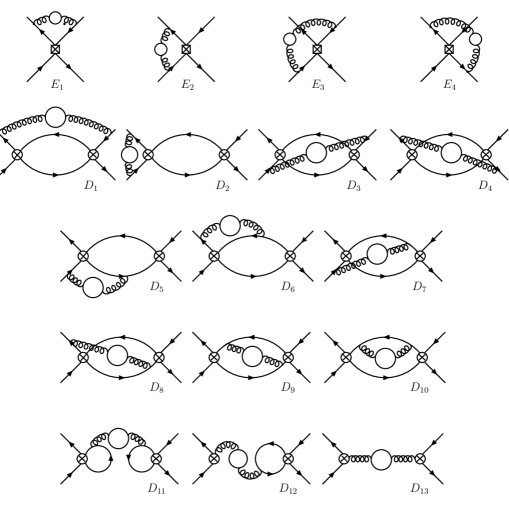
Figure 3: Diagrams with $O_{1,2}$ or $O_{8}$ contributing to the ${\cal O}(\alpha_{s}^{2}N_{f})$ corrections to $\Delta\Gamma$.

 

These diagrams are a gauge-invariant subset of all NNLO diagrams and grow with the number $N_{f}$ of active quark flavours. (In $b$ decays one has $N_{f}=5$.) Note that diagrams involving $O_{8}$ have less than three loops, because the definition of $O_{8}$ in Eq. (4) involves one power of the strong coupling $g_{s}$. We have also calculated the contributions with penguin operators $O_{3-6}$ [1], counting their small Wilson coefficients as ${\cal O}(\alpha_{s})$ [17], so that also here only one-loop and two-loop diagrams are needed.

In the calculation one can neglect the charm mass on the lines attached to a $O_{1,2}$ vertex, because the associated error is of order $m_{c}^{2}/m_{b}^{2}$, i.e. 5% of the expected ${\cal O}(15\%)$ NNLO correction. A charm quark running in the closed quark loop in the gluon propagator, however, leads to a term linear in $m_{c}/m_{b}$, so that we have kept a non-zero charm mass there.

For illustration we show the charm-loop contribution to the coefficient multiplying $C_{2}^{2}$ in the NNLO correction to $\widetilde{G}_{S}$:

$$F^{(2),N_{V}}_{S,22}(z)= -9.01785\log\frac{\mu_{1}}{m_{b}}-11.8519\log\frac{\mu_{2}}{m_{b}}-14.2222\log\frac{\mu_{1}}{m_{b}}\log\frac{\mu_{2}}{m_{b}}+10.6667\log^{2}\frac{\mu_{1}}{m_{b}}$$

$$+7.11111\log^{2}\frac{\mu_{2}}{m_{b}}-42.0084+105.276\frac{m_{c}}{m_{b}}+{\cal O}\left(\frac{m_{c}^{2}}{m_{b}^{2}}\right)$$

Displaying only the error from the $\mu_{1}$ dependence, our NLO and large-$N_{f}$ NNLO results read

$$\Delta\Gamma^{NLO} =\left(0.091\pm 0.020_{\rm scale}\right)\,\,\mbox{GeV}\qquad\mbox{(pole)}$$

$$\Delta\Gamma^{NLO} =\left(0.104\pm 0.015_{\rm scale}\right)\,\,\mbox{GeV}\qquad\mbox{($\overline{\rm MS}$)}$$ (8)

$$\Delta\Gamma^{NNLO} =\left(0.108\pm 0.021_{\rm scale}\right)\,\,\mbox{GeV}\qquad\mbox{(pole)}$$

$$\Delta\Gamma^{NNLO} =\left(0.103\pm 0.015_{\rm scale}\right)\,\,\mbox{GeV}\qquad\mbox{($\overline{\rm MS}$)}$$ (9)

Note that we have used a different implementation of the $\overline{\rm MS}$ scheme here: In Eq. (7) the prefactor in Eq. (6) is chosen with $\bar{m}_{b}^{2}(\mu_{1})$ and the $\mu_{1}$ dependence of this factor nicely cancels with the one in $G^{\prime}$ and $\widetilde{G}_{S}$, and this feature seems to be accidental. If one chooses $\bar{m}_{b}^{2}(\bar{m}_{b})$ instead (with properly adjusted $\mu_{1}$ terms in $G^{\prime}$ and $\widetilde{G}_{S}$), one finds the larger $\mu_{1}$ dependence of Eq. (8). Our partial NNLO correction is sizable in the pole scheme and lifts the result closer to the $\overline{\rm MS}$ result. In the $\overline{\rm MS}$ scheme instead our large-$N_{f}$ correction is very small and unlikely to be the dominant piece of the full NNLO result.

The large $N_{f}$ limit of QCD spoils asymptotic freedom, because the $\beta$ function changes sign for sufficiently large values of $N_{f}$. One may remedy this by “naive non-Abelianisation (NNA)”, which means to trade $N_{f}$ for the leading coefficient $\beta_{0}=11-2/3N_{f}$ of the QCD $\beta$ function [27, 26]. This procedure flips the sign of the NNLO correction leading to

$$\Delta\Gamma^{NNA} =\left(0.071\pm 0.020_{\rm scale}\right)\,\,\mbox{GeV}\qquad\mbox{(pole)}$$

$$\Delta\Gamma^{NNA} =\left(0.099\pm 0.012_{\rm scale}\right)\,\,\mbox{GeV}\qquad\mbox{($\overline{\rm MS}$)}.$$ (10)

In applications like ours, in which the size of the NNLO correction depends on the chosen renormalisation scheme for the Wilson coefficients, it is not clear whether NNA improves the result. E.g. in Ref. [28] it has been found that the $\alpha_{s}^{2}\beta_{0}$ term is not a good approximation to the full NNLO result to the calculated quantity.

3 Conclusions

The calculation of the $\alpha_{s}^{2}N_{f}$ terms of the NNLO correction to $\Delta\Gamma$ has reduced the renormalisation scheme dependence of the theory prediction and has moved the pole scheme result close to the $\overline{\rm MS}$ result. But there is no progress in the reduction of the dependence on the renormalisation scale and the correction found in the $\overline{\rm MS}$ scheme is too small to be the dominant part of the full NNLO result. Therefore a complete NNLO calculation is needed. In the meantime, we advocate for the use of the $\overline{\rm MS}$ result with a conservative perturbative error [1]:

$$\Delta\Gamma =\left(0.104\pm 0.015_{\rm scale}\pm 0.007_{B,\widetilde{B}_{S}}\pm 0.015_{\Lambda_{\textit{\scriptsize{QCD}}}/m_{b}}\right)\,\,\mbox{GeV}\qquad\mbox{($\overline{\rm MS}$)}.$$ (11)

Acknowledgements

I thank Hrachia Asatrian, Artyom Hovhannisyan, and Arsen Yeghiazaryan for the fruitful collaboration on the project. The presented work has been supported by the German Bundesministerium für Bildung und Forschung (BMBF) under contract no. 05H15VKKB1 and by VolkswagenStiftung with grant no. 86426.

References

- [1] H. M. Asatrian, A. Hovhannisyan, U. Nierste and A. Yeghiazaryan, “Towards next-to-next-to-leading-log accuracy for the width difference in the system: fermionic contributions to order and ”, JHEP 1710 (2017) 191 [arXiv:1709.02160 [hep-ph]].
- [2] Heavy Flavor Averaging Group (HFLAV), https://hflav.web.cern.ch.
- [3] A. Abulencia et al. [CDF Collaboration], “Observation of Oscillations,” Phys. Rev. Lett. 97 (2006) 242003 [hep-ex/0609040].
- [4] R. Aaij et al. [LHCb Collaboration], “Precision measurement of the - oscillation frequency with the decay ,” New J. Phys. 15 (2013) 053021 [arXiv:1304.4741].
- [5] R. Aaij et al. [LHCb Collaboration], “Precision measurement of violation in decays,” Phys. Rev. Lett. 114 (2015) no.4, 041801 [arXiv:1411.3104].
- [6] R. Aaij et al. [LHCb Collaboration], “First study of the CP -violating phase and decay-width difference in decays,” Phys. Lett. B 762 (2016) 253 [arXiv:1608.04855].
- [7] G. Aad et al. [ATLAS Collaboration], “Measurement of the CP-violating phase and the meson decay width difference with decays in ATLAS,” JHEP 1608 (2016) 147 [arXiv:1601.03297].
- [8] V. Khachatryan et al. [CMS Collaboration], “Measurement of the CP-violating weak phase and the decay width difference using the B(1020) decay channel in pp collisions at 8 TeV,” Phys. Lett. B 757 (2016) 97 [arXiv:1507.07527].
- [9] T. Aaltonen et al. [CDF Collaboration], “Measurement of the Bottom-Strange Meson Mixing Phase in the Full CDF Data Set,” Phys. Rev. Lett. 109 (2012) 171802 [arXiv:1208.2967].
- [10] M. A. Shifman and M. B. Voloshin, in: Heavy Quarks ed. V. A. Khoze and M. A. Shifman, “Heavy Quarks,” Sov. Phys. Usp. 26 (1983) 387.
- [11] M. A. Shifman and M. B. Voloshin, “Preasymptotic Effects In Inclusive Weak Decays Of Charmed Particles,” Sov. J. Nucl. Phys. 41 (1985) 120 [Yad. Fiz. 41 (1985) 187];
- [12] M. A. Shifman and M. B. Voloshin, “Hierarchy Of Lifetimes Of Charmed And Beautiful Hadrons,” Sov. Phys. JETP 64 (1986) 698 [Zh. Eksp. Teor. Fiz. 91 (1986) 1180];
- [13] I. I. Bigi, N. G. Uraltsev and A. I. Vainshtein, “Nonperturbative corrections to inclusive beauty and charm decays: QCD versus phenomenological models,” Phys. Lett. B 293 (1992) 430 [hep-ph/9207214] [Erratum ibid. Phys. Lett. B 297 (1992) 477].
- [14] M. Gorbahn and U. Haisch, “Effective Hamiltonian for non-leptonic decays at NNLO in QCD,” Nucl. Phys. B 713 (2005) 291 [hep-ph/0411071].
- [15] M. Gorbahn, U. Haisch and M. Misiak, “Three-loop mixing of dipole operators,” Phys. Rev. Lett. 95 (2005) 102004 [hep-ph/0504194].
- [16] M. Beneke, G. Buchalla and I. Dunietz, “Width Difference in the System,” Phys. Rev. D 54 (1996) 4419 [hep-ph/9605259] [Erratum ibid. Phys. Rev. D 83 (2011) 119902].
- [17] M. Beneke, G. Buchalla, C. Greub, A. Lenz and U. Nierste, “Next-to-leading order QCD corrections to the lifetime difference of mesons,” Phys. Lett. B 459 (1999) 631 [hep-ph/9808385].
- [18] M. Ciuchini, E. Franco, V. Lubicz, F. Mescia and C. Tarantino, “Lifetime differences and CP violation parameters of neutral B mesons at the next-to-leading order in QCD,” JHEP 0308 (2003) 031 [hep-ph/0308029].
- [19] M. Beneke, G. Buchalla, A. Lenz and U. Nierste, “CP asymmetry in flavor specific B decays beyond leading logarithms,” Phys. Lett. B 576 (2003) 173 [hep-ph/0307344].
- [20] A. Lenz and U. Nierste, “Theoretical update of mixing,” JHEP 0706 (2007) 072 [hep-ph/0612167].
- [21] A. Bazavov et al. [Fermilab Lattice and MILC Collaborations], “-mixing matrix elements from lattice QCD for the Standard Model and beyond,” Phys. Rev. D 93 (2016) no.11, 113016 [arXiv:1602.03560].
- [22] T. Mannel, B. D. Pecjak and A. A. Pivovarov, “Sum rule estimate of the subleading non-perturbative contributions to mixing,” Eur. Phys. J. C 71 (2011) 1607 [hep-ph/0703244 [HEP-PH]].
- [23] C. Davies, J. Harrison, G. P. Lepage, C. Monahan, J. Shigemitsu and M. Wingate, “Improving the theoretical prediction for the width difference: matrix elements of next-to-leading order operators,” EPJ Web Conf. 175 (2018) 13023. [arXiv:1712.09934 [hep-lat]].
- [24] I. Dunietz, R. Fleischer and U. Nierste, “In pursuit of new physics with decays,” Phys. Rev. D 63 (2001) 114015 [hep-ph/0012219].
- [25] S. Jäger, M. Kirk, A. Lenz and K. Leslie, “Charming new physics in rare B-decays and mixing?,” Phys. Rev. D 97 (2018) no.1, 015021 [arXiv:1701.09183 [hep-ph]].
- [26] M. Beneke and V. M. Braun, “Naive non-Abelianization and resummation of fermion bubble chains,” Phys. Lett. B 348 (1995) 513 [hep-ph/9411229].
- [27] S. J. Brodsky, G. P. Lepage and P. B. Mackenzie, “On the Elimination of Scale Ambiguities in Perturbative Quantum Chromodynamics,” Phys. Rev. D 28 (1983) 228.
- [28] H. M. Asatrian, T. Ewerth, A. Ferroglia, C. Greub and G. Ossola, “Complete contribution to at order ,” Phys. Rev. D 82, 074006 (2010) [arXiv:1005.5587].