Simulations of wobble damping in viscoelastic rotators

Abstract

Using a damped mass-spring model, we simulate wobble of spinning homogeneous viscoelastic ellipsoids undergoing non-principal axis rotation. Energy damping rates are measured for oblate and prolate bodies with different spin rates, spin states, viscoelastic relaxation timescales, axis ratios, and strengths. Analytical models using a quality factor by Breiter et al. (2012) and for the Maxwell rheology by Frouard & Efroimsky (2018) match our numerical measurements of the energy dissipation rate after we modify their predictions for the numerically simulated Kelvin-Voigt rheology. Simulations of nearly spherical but wobbling bodies with hard and soft cores show that the energy dissipation rate is more sensitive to the material properties in the core than near the surface.

1 Introduction

Increasingly large multiple epoch photometric surveys, giving light curves with many data points, are adding to the population of asteroids and comets with rotational measurements (e.g., Warner et al. 2009; Masiero et al. 2009; Waszczak et al. 2015; Vaduvescu et al. 2017; Chang et al. 2017). The recent discovery of Interstellar object 1I/2017 U1 ’Oumuamua with extreme axis ratios and non-principal axis rotation (Meech et al., 2017; Drahus et al., 2018; Fraser et al., 2018; Belton et al., 2018) motivates studying wobble damping in elongated bodies. About 1 of 100 asteroids in the Asteroid Light Curve Database (LCDB) (Warner et al., 2009) are identified as non-principal axis rotators (Pravec et al., 2014).

Development of a viscoelastic mass spring model for spinning gravitating bodies (Quillen et al., 2016a; Frouard et al., 2016; Quillen et al., 2016b, 2017, 2019b; Quillen et al., 2019a) allows us to numerically study spin evolution with a code that directly relates simulated material strength and dissipation rate to variations in the spin state. Our numerical simulations are complimentary to analytic computations of the wobbling or precession damping rate (Burns & Safronov, 1973; Sharma et al., 2005; Efroimsky & Lazarian, 2000; Breiter et al., 2012; Frouard & Efroimsky, 2018). Moreover, the simulations are flexible as they can be used to model complex body shapes (e.g., Quillen et al. 2019b), bodies with inhomogeneous internal composition (e.g., Quillen et al. 2016b) and the distribution of internally dissipated heat (e.g., Quillen et al. 2019a).

At a given total rotational angular momentum, the most stable rotational state of a rigid object is that with the least rotational kinetic energy. This corresponds to the rotation about the axis of maximum moment of inertia or about its shortest principal body axis. A body that is initially rotating about a principal axis can be rotationally excited due to out-gassing (if a comet, Marsden et al. 1973), an impact (e.g., Paolicchi et al. 2002), internal shape changes (Sánchez & Scheeres, 2018), or applied external torques such as a gravitational torque during a close approach with another massive object, (e.g., Scheeres et al. 2000). If the rotation axis differs from a principal body axis, the spin state is described as a non-principal axis (NPA) rotation state. NPA rotational states are also known in the literature as complex rotational states or objects that are tumbling or wobbling.

Due to cyclic variations in stresses and strains, an object in an NPA state slowly looses kinetic energy (Prendergast, 1958). For an object to be in an NPA state, the damping timescale due to dissipation or mechanical friction must be larger than either the time elapsed since the last spin excitation event (e.g., such as an asteroid impact) or a time scale associated with rotational excitation by another process, such as out-gassing. Some well studied small bodies are in NPA states. Examples are Comet 1P/Halley (e.g., Belton et al. 1991; Samarasinha et al. 1991) asteroid 4179 Toutatis (Hudson & Ostro, 1995), asteroid 99942 Apophis (Pravec et al., 2014) and Interstellar object 1I/2017 U1 ’Oumuamua (Drahus et al., 2018; Fraser et al., 2018; Belton et al., 2018).

An estimate for the damping timescale for a wobbling spinning body is

$$\tau\sim\frac{\mu Q}{\rho Kr_{n}^{2}\Omega^{3}},$$ (1)

(Burns & Safronov, 1973) where $r_{n}$ is an average radius, $\rho$ is a bulk density, $\mu$ is a shear modulus, $Q$ is an energy dissipation factor, also called a quality factor, and $\Omega$ the spin rate. The scaling factor $K$ takes into account body shape and initial spin state. The product $\mu Q\sim 10^{11}$ Pa is representative of small solar system bodies (Harris, 1994; Pravec et al., 2014). In the body’s reference frame of a homogeneous body with rotational symmetry, such as an oblate or prolate ellipsoid, the spin axis precesses with a single frequency about the body’s axis of symmetry. This precession frequency gives the period for stress-strain cycling within the asteroid. The energy dissipation parameter $Q$ (also called the quality factor) describes the fraction of energy lost per spin or spin precession period (Efroimsky & Lazarian, 2000; Sharma et al., 2005; Breiter et al., 2012). More generally, the energy dissipation rate in a wobbling body is a function of the current spin rate and state, the ratios between the body’s three moments of inertia and the rheology. If a body has three different moments of inertia (e.g., is a triaxial ellipsoid), the spin vector in the body frame expanded in Fourier series contains multiple frequency components. The frequency dependence of the energy dissipation rate affects the wobble damping timescale so triaxial bodies are more difficult to model than prolate or oblate ellipsoids of revolution (Efroimsky & Lazarian, 2000; Sharma et al., 2005; Breiter et al., 2012; Frouard & Efroimsky, 2018).

The paucity of asteroids above a spin limit of 2.2 hours and distribution of body axis ratios at each spin period, requiring shear strength but little tensile strength, has lead to a granular aggregate or rubble pile interpretation of asteroid composition (Walsh, 2018). Wobble damping computations assume that spin associated accelerations cause small variations in strain and that the body is ‘prestressed’ by its own self-gravity (Sharma et al., 2005). The prestressing means that cohesive forces between grains are not necessarily required for elastic behavior. In this context the elastic shear modulus, $\mu$, characterizes variations in the repulsive elastic contacts between grains, pebbles and boulders about the mean stress field. There is considerable uncertainty about the viscoelastic behavior of asteroid material. A strong pressure pulse in asteroid material could be rapidly attenuated, as they are in laboratory granular materials (O’Donovan et al., 2016) and giving a low $Q$ for stress strain cycling. Alternatively, seismic attenuation rates are long in lunar regolith (Dainty et al., 1974; Toksöz et al., 1974; Nakamura, 1976) compared to typically seen on the Earth and if asteroid material acts like lunar regolith it might have a large $Q$ of a few thousand. The P and S-wave speeds in a loose granular material could depend upon pressure and porosity (Hostler, 2005).

Going beyond a $Q$ quality factor description of energy dissipation, Frouard & Efroimsky (2018) have calculated the wobbling damping, or nutation damping timescale for homogeneous oblate ellipsoids that obey a Maxwell viscoelastic rheology. They found that the energy dissipation rate and associated tumbling damping timescale is primarily a function of viscosity $\eta$ with $1/\eta$ replacing the ratio of a spin frequency to the shear modulus times the quality factor, $\mu Q$, in the predicted dissipation rate. Their theory can be extended for any linear rheology, where there is a linear relation between stress and strain.

Instead of analytically computing the dissipation rate (as did Efroimsky & Lazarian 2000; Sharma et al. 2005; Breiter et al. 2012; Frouard & Efroimsky 2018), we directly simulate wobble damping in an extended body using an N-body and mass-spring model. The mass-spring model is an N-body simulation technique of low computational complexity (Quillen et al., 2016a; Frouard et al., 2016). As spring forces are applied between pairs of point particles, the simulation accurately conserves angular momentum. Since the strain of a spring is computed from the distance between a pair of point particles, the simulations can measure extremely small levels of strain. Thus mass-spring N-body models are an attractive method for simulating rotational dynamics. Because our mass-spring model adds both spring damping forces and spring elastic forces on pairs of particles, our model approximates a Kelvin-Voigt viscoelastic rheology (Frouard et al., 2016) rather than the Maxwell rheology studied by Frouard & Efroimsky (2018). Dissipation rates as a function of frequency can be compared between the two viscoelastic models using the complex compliances for each model, relating stress to strain as a function of frequency (e.g., see appendix D by Frouard & Efroimsky 2018).

The discovery of active asteroids P/2013 R3 and P/2013 P5 (Jewitt et al., 2013, 2014) motivates the study of the disruption of inhomogeneous self-gravitating aggregates. Following Yarkovsky-O’Keefe-Radzievskii-Paddack effect (YORP) induced spin increase, the mode of deformation or disruption depends on the strength, density and cohesion of an internal core, compared to that of a shell (Hirabayashi, 2014; Hirabayashi & Scheeres, 2015; Hirabayashi et al., 2015; Scheeres, 2015; Sánchez & Scheeres, 2018). Asteroids may host a surface layer of more highly dissipative regolith over a harder, less dissipative but fractured core (Nimmo & Matsuyama, 2017). In our previous study of tidal spin down of triaxial ellipsoids undergoing principal axis rotation, we found that the energy distribution rate was sensitive to small volumes of low strength material (Quillen et al., 2016b). Internal variations in strength and viscosity should also affect the wobble damping rates. Our code is not restricted to homogeneous material properties or ellipsoidal shapes so we can numerically explore the sensitivity of wobble damping to core strength.

In this paper we describe our simulations in section 2. We discuss numerical measurements of energy dissipation rates for homogeneous ellipsoids undergoing NPA rotation. In section 3, we modify the predictions by Frouard & Efroimsky (2018); Breiter et al. (2012) for our simulated viscoelastic rheology and compare them to our numerically measured dissipation rates. In section 4, we discuss numerical experiments on inhomogeneous bodies. A summary and discussion follows in section 5. Nomenclature is summarized in Table 1.

2 Elastic Body Simulations

2.1 Mass-spring models

To simulate energy dissipation and spin evolution of a non-spherical body in a non-principal axis rotation state, we use a mass-spring model (Quillen et al., 2016a; Frouard et al., 2016; Quillen et al., 2016b, 2017), that is built on the modular N-body code rebound (Rein & Liu, 2012). A viscoelastic solid is approximated as a collection of mass nodes that are connected by a network of springs. Springs between mass nodes are damped and the spring network approximates the behavior of a Kelvin-Voigt viscoelastic solid with Poisson ratio of 1/4 (Kot et al., 2015). When a large number of particles is used to resolve the spinning body, and with many springs in the spring-network, the mass-spring model behaves like an isotropic continuum elastic solid (Kot et al., 2015), including its ability to transmit seismic waves and vibrate in normal modes (Quillen et al., 2019b).

The mass particles or nodes in the resolved spinning body are subjected to three types of forces: the gravitational forces acting on every pair of particles in the body, and the elastic and damping spring forces acting only between sufficiently close particle pairs. As all forces are applied equal and oppositely to pairs of point particles and along the direction of the vector connecting the pair, momentum and angular momentum conservation are assured. Springs have a spring constant $k_{s}$ and a damping rate parameter $\gamma_{s}$. The number density of springs, spring constants and spring lengths set the shear modulus, $\mu$, whereas the spring damping rate, $\gamma_{s}$, sets the shear viscosity, $\eta$, and viscoelastic relaxation time, $\tau_{\rm relax}=\eta/\mu$. For a Poisson ratio of 1/4, the Young’s modulus $E=2(1+\nu)\mu=2.5\mu$. The equation we used to calculate Young’s $E$ from the spring constants of the springs in our code is equation 29 by Frouard et al. (2016) and originally derived by Kot et al. (2015). The equation we used to calculate viscosity $\eta$ from the spring damping coefficients $\gamma_{s}$ is equation 31 by Frouard et al. (2016). Our simulated material is compressible, so energy damping arises from both deviatoric and volumetric stresses. Springs are created at the beginning of the simulation and do not grow or fail during the simulation, so there is no plastic deformation.

We work with mass in units of $M$, the mass of the asteroid, distances in units of volumetric radius, $R_{\rm vol}$, the radius of a spherical body with the same volume, and time in units of $t_{\rm grav}$ (equation 2).

$$t_{\rm grav} \equiv\sqrt{\frac{R_{\rm vol}^{3}}{GM}}=\sqrt{\frac{3}{4\pi G\rho}}$$

$$=1685{\rm s}\left(\frac{\rho}{1260\ {\rm kg\ m}^{3}}\right)^{-\frac{1}{2}}.$$ (2)

The density in these units is

$$\rho=\frac{3}{4\pi}.$$ (3)

A convenient unit of energy density

$$e_{\rm grav}=\frac{GM^{2}}{R_{\rm vol}^{4}}=110\ {\rm kPa}\left(\frac{M}{7.8\times 10^{10}{\rm kg}}\right)^{2}\left(\frac{R_{\rm vol}}{246\ {\rm m}}\right)^{-4}.$$ (4)

Elastic moduli, such as shear modulus $\mu$ and Young’s modulus $E$, are given in units of $e_{\rm grav}$ (equation 4) which scales with the gravitational energy density or central pressure. All mass nodes have the same mass and all springs have the same spring constants. For numerical stability, the simulation time-step must be chosen so that it is shorter than the time it takes elastic waves to travel between nodes (Frouard et al., 2016; Quillen et al., 2016b).

Initial node distribution and spring network is chosen with the triaxial ellipsoid random spring model described by Frouard et al. (2016); Quillen et al. (2016b). The surface obeys $\frac{x^{2}}{a^{2}}+\frac{y^{2}}{b^{2}}+\frac{z^{2}}{c^{2}}=1$ with $a,b,c$ equal to half the lengths of the principal body axes. An oblate ellipsoid is described with an axis ratio $c/a<1$ and $b=a$ and has a pancake-like shape. A prolate ellipsoid has $c/a<1$ and $c=b$ and has a cigar-like shape. Oblates and prolates are sometimes described as ‘biaxial’ or as ‘ellipsoids of revolution’. Particle positions within a cube containing the body’s surface are drawn from a uniform spatial distribution but only accepted as mass nodes into the spring network if they are within the shape model and if they are more distant than $d_{I}$ from every other previously generated particle. Once the particle positions have been generated, every pair of particles within distance $d_{s}$ of each other are connected with a single spring. The parameter $d_{s}$ is the maximum rest length of any spring. We chose $d_{s}/d_{I}$ so that the number of springs per node is greater than 12, as recommended by Kot et al. (2015), so as to better approximate a homogenous and isotropic elastic solid. Springs are initiated at their rest lengths. The body is not initially in equilibrium because the body will slightly compress due to self-gravity. (All mass nodes exert gravitational forces on each other during the simulation.) We begin each simulation with an increased damping parameter. The simulations are run for a time $t_{\rm damp}$ to remove vibrations as the body settles into an equilibrium state. After this damping period we set the spring damping parameter to the desired value (for the simulation). Measurements are only done on the simulation output after this time.

$\begin{array}[]{c}\includegraphics[width=216.81pt,trim=0.0pt 0.0pt 0.0pt 0.0pt,clip]{oblate.png}\\ \includegraphics[width=216.81pt,trim=0.0pt 0.0pt 0.0pt 0.0pt,clip]{prolate.png}\end{array}$

Figure 1: Top panel: A simulation snap-shot of an oblate spinning body. Bottom panel: A simulation snapshot of a prolate spinning body. The oblate axis ratio is $a:c=$ 1:0.33 with $a=b$ and the prolate axis ratio is $a:c=$ 1:0.33 with $b=c$. These are snapshots taken from the simulations while they were running. The angular momentum vector points upward and they are undergoing non-principal axis rotation (NPA).

Table 1: Some Nomenclature

Non-principal axis	NPA
Damping timescale	$\tau$
Asteroid mass	$M$
Radius of equivalent volume	$R_{\rm vol}$
Mass density	$\rho$
Semi-axes of ellipsoid	$a,b,c$
Body axis ratio if oblate or prolate	$h$
Spin vector	$\boldsymbol{\Omega}$
Initial spin vector	${\boldsymbol{\Omega}}_{0}$
Wobble or NPA angle	$\theta$
Angle between ${\boldsymbol{\Omega}}$ and axis of symmetry	$\alpha$
Moment of inertia parallel to body symmetry axis	$I_{\parallel}$
Moment of inertia perpendicular to body symmetry axis	$I_{\perp}$
Angular momentum vector	$\bf J$
Final spin if oblate	$\tilde{\omega}$
Precession rate in body frame	$\omega_{\rm prec}$
Shear modulus	$\mu$
Young’s modulus	$E$
Viscosity	$\eta$
Viscoelastic relaxation time	$\tau_{\rm relax}$
Poisson ratio	$\nu$
Kelvin-Voigt viscoelastic model	KV
Maxwell viscoelastic model	MW
Frouard & Efroimsky (2018)	FE
Breiter et al. (2012)	BR
Quality factor	$Q$
Stress	$\sigma$
Strain	$\epsilon$

Notes: $\tilde{\omega}$ is not equal to the final spin value (when principal axis rotation is reached) if the body is prolate.

2.2 Body Frame Precession frequency for homogeneous oblate and prolate ellipsoids

Acceleration in the body frame depends on the precession frequency. We outline notation for computation of this frequency for ellipsoids of rotation following Sharma et al. (2005); Frouard & Efroimsky (2018). In the body frame, our coordinate system is defined by the three principal axes of inertia with coordinates $x,y,z;$ and with unit vectors ${\bf e}_{x},{\bf e}_{y},{\bf e}_{z}$. The angular velocity is denoted by ${\boldsymbol{\Omega}}$ and the spin angular momentum is $\bf J$. The motion of a free rigid body is given by Euler equations

$$I_{i}\dot{\Omega}_{i}=(I_{j}-I_{k})\Omega_{j}\Omega_{k}$$ (5)

with $(i,j,k)=(x,y,z)$ and cyclic transpositions $(i,j,k)=(y,z,x)$ and $(i,j,k)=(z,x,y)$.

We consider a free spinning homogeneous oblate or prolate ellipsoid of revolution with semi-axes $a,b,c$. For an oblate $a=b>c$ and for a prolate $a>b=c$. We assume that the body’s axis of symmetry is aligned with ${\bf e}_{z}$, with moment of inertia $I_{\parallel}$. For prolate and oblate ellipsoids,

$$I_{\parallel} =\frac{2Ma^{2}}{5}\qquad{\rm oblate}$$

$$I_{\parallel} =\frac{2Mc^{2}}{5}\qquad{\rm prolate}$$ (6)

The other two axes have the same moment of inertia $I_{\perp}$. We use axis ratio $h$ with convention

$$h =\frac{c}{a}<1\qquad{\rm oblate}$$

$$h =\frac{a}{c}>1\qquad{\rm prolate},$$ (7)

giving

$$I_{\perp} =\frac{1+h^{2}}{2}I_{\parallel}$$ (8)

for both prolate and oblate ellipsoids.

In the body frame, the angular momentum vector $\bf J$ and spin vector $\boldsymbol{\Omega}$ are both precessing with frequency $\omega_{\rm prec}$ about the body’s axis of symmetry. Euler’s equations give a constant $\Omega_{z}$ and

$$\dot{\boldsymbol{\Omega}} =-\left(\frac{1-h^{2}}{1+h^{2}}\right)\Omega_{z}\left[-\Omega_{y}{\bf e}_{x}+\Omega_{x}{\bf e}_{y}\right].$$ (9)

The factor $-(1-h^{2})/(1+h^{2})=(I_{\perp}-I_{\parallel})/I_{\perp}$ and

$$\Omega_{x} =\Omega\sin\alpha\cos(\omega_{\rm prec}t)$$

$$\Omega_{y} =\Omega\sin\alpha\sin(\omega_{\rm prec}t)$$

$$\Omega_{z} =\Omega\cos\alpha=\frac{J}{I_{\parallel}}\cos\theta$$ (10)

where $\alpha$ is the angle between spin $\boldsymbol{\Omega}$ and body axis ${\bf e}_{z}$, and $\theta$ is the angle between angular momentum $\bf J$ and body axis ${\bf e}_{z}$. This angle is sometimes called the non-principal angle or wobble angle and it is one of the Andoyer-Deprit canonical variables (Celletti, 2010). The angle $\alpha$ and NPA angle $\theta$ are related by

$$\tan\theta=\frac{I_{1}}{I_{3}}\tan\alpha=\frac{1+h^{2}}{2}\tan\alpha.$$ (11)

We define the frequency (following Sharma et al. 2005; Frouard & Efroimsky 2018)

$$\tilde{\omega} \equiv\frac{J}{I_{\parallel}}.$$ (12)

Our $\tilde{\omega}$ is equivalent to $\Omega_{0}$ defined by Sharma et al. (2005) and $\tilde{\omega}_{3}$ defined by Frouard & Efroimsky (2018). This is the final spin rate of a homogenous oblate ellipsoid that has damped down to principal axis rotation while conserving angular momentum. Equation 9 implies that the precession frequency (for both prolate and oblate ellipsoids)

$$\omega_{\rm prec} =\left(\frac{I_{\parallel}}{I_{\perp}}-1\right)\Omega_{z}=\left(\frac{1-h^{2}}{1+h^{2}}\right)\frac{J}{I_{\parallel}}\cos\theta$$

$$=\left(\frac{1-h^{2}}{1+h^{2}}\right)\cos\theta\ \tilde{\omega}.$$ (13)

The frequency $\omega_{\rm prec}$ is the precession rate of spin vector $\boldsymbol{\Omega}$ and angular momentum vector $\bf J$ in the body frame. The frequency $\Omega_{z}$ (equation 10) is equivalent to $\Omega_{3}$ used by Frouard & Efroimsky (2018).

Using equations 10, 11, 12 and 13 it is convenient to write spin components in terms of $\tilde{\omega}$ and NPA angle $\theta$

$$\Omega_{x} =\tilde{\omega}\frac{2}{1+h^{2}}\sin\theta\ \cos\omega_{\rm prec}t$$ (14)

$$\Omega_{y} =\tilde{\omega}\frac{2}{1+h^{2}}\sin\theta\ \sin\omega_{\rm prec}t$$ (15)

$$\Omega_{z} =\tilde{\omega}\cos\theta.$$ (16)

We will use these expressions to generate initial conditions for our simulations.

Here we have defined $\theta$ in terms of angle between angular momentum and the body’s axis of symmetry not the principal axis with the largest moment of inertia. For oblate bodies there is no difference between the two definitions. However prolate bodies reach principal axis rotation at $\theta=\pi/2$ rather than $\theta=0$. The precession frequency in the body frame ($\omega_{\rm prec}$) should not be confused with precession frequencies of Euler angles.

2.3 Measurements of Energy Dissipation rates

We run series of short simulations to measure energy dissipation rates for wobbling spinning bodies. To measure the dissipation rate in each numerical simulation we compute at each time-step the total energy. This is a sum of gravitational potential energy, the kinetic energy and the spring potential energies. We checked that without dissipation, the sum of gravitational potential energy, elastic potential energy and kinetic energy (including vibrational and rotational motions) was conserved. The simulations were integrated for a total time $t_{\rm max}$ which we chose to be between 100 and 400 (in our numerical units of $t_{\rm grav}$). For each simulation we plotted total energy versus time. In most cases the points lie on a line with energy decreasing with time and with slope giving the measurement of energy dissipation rate in gravitational units. However, bodies with slow precession rates took longer to reach an equilibrium state where the energy as a function of time was linearly decreasing. We discarded earlier outputs, retaining only energy measurements after the body has reached an equilibrium state and the energy as a function of time was linear. In many cases we saw low amplitude oscillations (in energy) at twice the body precession frequency along with a steady decrease in energy. For these we increased the total integration time so that it was more than a few times the precession frequency, making it possible to measure the energy decay rate slope. In all cases we measured slopes with a linear fit to the energy as a function of time. Each simulation took 10 to 25 minutes on a 2018 MacBook Pro with a 2.6 GHz Intel Core i7 processor.

Figure 1 shows snap shots of two of our simulations. The top snapshot shows an oblate ellipsoid and the bottom one a prolate ellipsoid. The angular momentum axis in both figures is upward. The green lines connecting the particles represent the springs. The gray spheres represent the point mass particle nodes. These illustrate the number of particles and springs in the simulations discussed in this manuscript.

Table 2 lists common simulation parameters. Parameters for individual simulations are listed in the subsequent tables.

We checked that precession rate in the body frame measured from the simulation was equal to that given by formula 13 for oblate and prolate bodies. We keep $\omega_{\rm prec}\tau_{\rm relax}<1$ to remain in the low frequency viscoelastic regime. If we go in the other direction $\omega_{\rm prec}\tau_{\rm relax}>1$ then the Kelvin Voigt model would resemble the Maxwell viscoelastic model. We prefer to work in the lower limit as this gives a model with weak rather than strong damping in each spring.

Table 2: Common Simulation Parameters

Common simulation parameters
Radius of equivalent volume	$R_{\rm vol}$	1
Mass	$M$	1
Density	$\rho$	$\frac{3}{4\pi}$
Gravitational timescale	$t_{\rm grav}$	1
Timestep	$dt$	0.005
Minimum distance between mass nodes	$d_{I}$	0.12
Ratio of max spring length to $d_{I}$	$d_{s}/d_{I}$	2.3
Number of nodes	$N_{\rm nodes}$	$\approx 1800$
Number of springs per node	$N_{\rm springs}/N_{\rm nodes}$	$\approx 13$
Damping time	$t_{\rm damp}$	10
Simulation time	$t_{\rm max}$	100–400

Note: Units in this table and subsequent tables are in N-body or gravitational units, as described in section 2.1.

3 Simulations of Oblate and Prolate ellipsoids

We describe a series of simulations that varies body axis ratios and spin axes with the goal of checking equation 57 Frouard & Efroimsky (2018) and the similar equation 103 by Breiter et al. (2012)) for the power dissipated by a homogenous viscoelastic oblate body undergoing NPA rotation. In section 3.1 we discuss how the energy dissipation rate depends on the viscoelastic relaxation timescale. In section 3.2 we explore how the energy dissipation rate depends depends on spin rate. In section 3.3 and 3.4 we explore how the dissipation rates are sensitive to NPA angle $\theta$ and axis ratio $h$ for oblate and prolate ellipsoids.

Table 3: Oblate ellipsoid simulation parameters for varying viscoelastic relaxation time

Body shape		Oblate
Axis ratio	$h$	1/3
Spring constant	$k_{s}$	0.08
Shear modulus	$\mu$	$1.5$
Spring damping coefficients	$\gamma_{s}$	1/4, 1/2, 1, 2, 4, 8, 16
NPA angle	$\theta$	$39.3^{\circ}$
Initial spin	${\boldsymbol{\Omega}}_{0}$	(0.3, 0.0, 0.3)
Precession rate	$\omega_{\rm prec}$	0.243
Frequency	$\tilde{\omega}$	0.343
Relevant figure		Figure 2

Notes: We carried out a series of simulations with different spring damping coefficients. These simulations are discussed in section 3.1. Additional simulation parameters are listed in Table 2.

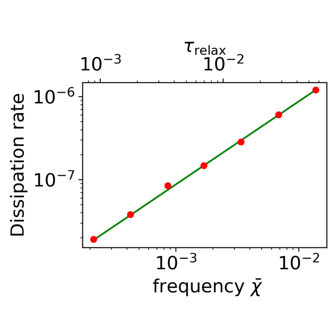
Figure 2: Dependence of dissipation rate during NPA rotation depends on viscoelastic relaxation time. We show energy dissipation rate measured for a series of simulations of wobbling oblate ellipsoids with parameters listed in Tables 2 and 3. The simulations are identical except the spring dissipation parameter $\gamma_{s}$ is varied. Numerical measurements are shown as red points. The bottom $x$ axis shows the frequency $\bar{\chi}=\tau_{\rm relax}\omega_{\rm prec}$, the top $x$ axis shows viscoelastic relaxation time $\tau_{\rm relax}$ and the $y$ axis shows the dissipated power. The green line is linear in $\tau_{\rm relax}$ or $\bar{\chi}$, as predicted for the Kelvin-Voigt viscoelastic model (with a slope of 1 on the log-log plot) and goes through the point on the lower left. The line was not fit to the measured dissipation rates but shows that the points are consistent with energy dissipation rate linear dependent on viscoelastic relaxation time $\tau_{\rm relax}$ or frequency $\bar{\chi}$, predicted for the Kelvin-Voigt model for small $\bar{\chi}$.

3.1 Sensitivity of the energy dissipation rate to viscoelastic relaxation timescale in the Kelvin-Voigt model

In continuum mechanics, an elastic/viscoelastic analogy, referred to as the correspondence principle, establishes a relation between frequency dependent stress and strain relations and the equivalent static relation by replacing the elastic shear modulus with a complex shear modulus (or, equivalently, by replacing the real shear compliance with a complex compliance) and by simultaneous replacing the real strain and stress with their Fourier harmonics. Frouard & Efroimsky (2018) computed the energy dissipation rate for wobbling oblate ellipsoids with a Maxwell rheology. The Maxwell rheology has complex shear rigidity (inverse of the complex compliance) as a function of frequency $\chi$

$$\tilde{\mu}(\chi)^{\rm MW}=\mu\frac{i\chi\tau_{\rm relax}}{1+i\chi\tau_{\rm relax}}=\mu\frac{i\bar{\chi}}{1+\bar{\chi}},$$ (17)

where $\tau_{\rm relax}=\eta/\mu$ is the viscoelastic relaxation timescale and $\bar{\chi}\equiv\chi\tau_{\rm relax}$ (see appendix D by Frouard & Efroimsky 2018 for an introduction to the correspondence principle). With stress $\sigma=\sigma_{0}\cos(\chi t)$, the energy dissipation rate per unit volume averaged over the oscillation period

$$p^{\rm MW}=\frac{1}{4\eta}\sigma_{0}^{2},$$ (18)

(equation D7 by Frouard & Efroimsky 2018) and is independent of frequency. As a result, their estimate for the total power dissipated for a wobbling oblate viscoelastic ellipsoid (equation 57 by Frouard & Efroimsky 2018)

$$P^{\rm FE,MW}_{\rm oblate}=\frac{a^{7}{\tilde{\omega}}^{4}\rho^{2}}{\eta}\left(f^{\rm FE}_{(1)}(h)\sin^{2}\theta\cos^{2}\theta+f^{\rm FE}_{(2)}(h)\sin^{4}\theta\right),$$ (19)

and does not directly depend on the precession frequency. Their functions

$$f^{\rm FE}_{(1)}(h) =\frac{\pi}{(h^{2}+1)^{4}}\frac{32}{315}(h^{2}+1)^{2}h^{5}\ \times$$

$$\ \ \Big{[}\frac{(1050h^{4}+2015h^{2}+507)}{(20h^{2}+13)^{2}}\Big{]}$$

$$f^{\rm FE}_{(2)}(h) =\frac{\pi}{(h^{2}+1)^{4}}\frac{16}{315}h\ \times$$

$$\ \ \Big{[}\frac{384h^{8}+960h^{6}+1900h^{4}+1650h^{2}+1125}{(8h^{4}+10h^{2}+15)^{2}}\Big{]}.$$ (20)

In contrast to equation 17, the Kelvin-Voigt viscoelastic model has complex shear modulus

$$\tilde{\mu}(\chi)^{\rm KV}=\mu(1+i\bar{\chi})$$ (21)

and time averaged energy dissipation rate per unit volume

$$p^{\rm KV}=\frac{1}{4\eta}\sigma_{0}^{2}\frac{{\bar{\chi}}^{2}}{1+{\bar{\chi}}^{2}}$$ (22)

(these are equations D3 and D8 by Frouard & Efroimsky 2018). The viscosity $\eta=\mu\tau_{\rm relax}$ for both Maxwell and Kelvin-Voigt viscoelastic models. In the limit of small ${\bar{\chi}}<1$

$$p^{\rm KV}\approx p^{\rm MW}\bar{\chi}^{2}.$$ (23)

The acceleration in the inertial frame is related to that in the body frame by

$$\frac{d{\bf a}}{dt}_{\rm inertial}=\frac{d{\bf a}}{dt}_{\rm body}+\dot{\boldsymbol{\Omega}}\times{\bf r}+{\boldsymbol{\Omega}}\times({\boldsymbol{\Omega}}\times{\bf r})$$ (24)

at position $\bf r$. As explained by Frouard & Efroimsky (2018), for an oblate or prolate body, the time dependence of $\boldsymbol{\Omega}$ depends on the precession frequency, $\omega_{\rm prec}$. However equation 24 shows that the acceleration contains Fourier components that depend on frequencies $\omega_{\rm prec}$ and $2\omega_{\rm prec}$. Using stress components calculated by Sharma et al. (2005), Frouard & Efroimsky (2018) integrated the time average of stress and stress for both Fourier frequencies and added the result to compute the total dissipated power. This accounts for the two terms in Equation 20 (from equation 57 by Frouard & Efroimsky 2018). Thus

$$P^{\rm FE,MW}_{\rm oblate}=P^{\rm FE}_{(1),{\rm oblate}}+P^{\rm FE}_{(2),{\rm oblate}}$$ (25)

where we have verified (by examining terms in the appendices by Frouard & Efroimsky (2018)) that the first term arises from the Fourier components of acceleration that depend on frequency $\omega_{\rm prec}$ (and is computed with $f^{\rm FE}_{(1)}(h)$) and the second term arises from those that depend on frequency $2\omega_{\rm prec}$ (and is computed with $f^{\rm FE}_{(2)}(h)$) .

Using frequencies ${\bar{\chi}}=\omega_{\rm prec}\tau_{\rm relax}$ and twice this, in the limit of small ${\bar{\chi}}<1$, and using equations 23 and 19, we estimate the total dissipated power for the Kelvin-Voigt model

$$P^{\rm FE,KV}_{\rm oblate} \approx\left(P^{\rm FE}_{(1),{\rm oblate}}+4P^{\rm FE}_{(2),{\rm oblate}}\right)\bar{\chi}^{2}$$

$$=\frac{a^{7}{\tilde{\omega}}^{4}\rho^{2}}{\eta}\omega_{\rm prec}^{2}\tau_{\rm relax}^{2}\times$$

$$\qquad\left(f^{\rm FE}_{(1)}(h)\sin^{2}\theta\cos^{2}\theta+4f^{\rm FE}_{(2)}(h)\sin^{4}\theta\right).$$ (26)

Note the factor of 4 on $f^{\rm FE}_{(2)}(h)$ arising from $2\bar{\chi}$.

We compare bodies with the same shear modulus $\mu$, body axis ratios, and initial spin vector but different viscosities. The dissipated power (equation 26)

$$P^{\rm KV}\propto\frac{\tau_{\rm relax}}{\mu},$$ (27)

where we have used viscosity $\eta=\mu\tau_{\rm relax}$. If we change the relaxation time $\tau_{\rm relax}$ in our simulations without changing the shear modulus, $\mu$, the body axis ratio, $h$, the angle $\theta$ or the initial body spin, $\boldsymbol{\Omega}$, and we maintain $\omega_{\rm prec}\tau_{\rm relax}<1$, then we expect to measure a linear relation between the viscoelastic relaxation timescale $\tau_{\rm relax}$ and the energy dissipation rate (as expected for the Kelvin-Voigt model). We can vary $\tau_{\rm relax}$ without varying these other quantities by adjusting the spring damping coefficients $\gamma_{s}$ and leaving other simulation parameters fixed.

Figure 2 shows a series of simulations of oblate bodies with all parameters identical except they have different values of spring dissipation parameter $\gamma_{s}$ and so they have different relaxation timescales $\tau_{\rm relax}$ and normalized frequencies $\bar{\chi}$. For these simulations the precession rates satisfy $\omega_{\rm prec}\tau<1$ so as to remain in the regime where $\bar{\chi}<1$ for equation 22 and giving an expected linear dependence of power on $\tau_{\rm relax}$ (as in equation 27). The parameters for these simulations are listed in Tables 2 and Table 3. We have plotted energy dissipation rate versus frequency $\bar{\chi}=\omega_{\rm prec}\tau$ (bottom $x$ axis) and viscoelastic relaxation time $\tau_{\rm relax}$ (top $x$ axis) in Figure 2 as red points, measured from for 7 simulations with $\gamma_{s}$ ranging from 1/4 to 16. We show a line in Figure 2 that has power $P\propto\bar{\chi}$. The line was not fit to the measured points but was adjusted to intersect the point on the lower left. The green line shows that dissipated power is proportional to $\bar{\chi}$, $\gamma_{s}$ and the viscoelastic relaxation time, as expected from equation 26 (with all other parameters remaining fixed). We confirm that the dissipation rate is proportional to the viscoelastic relaxation time with the Kelvin-Voigt model.

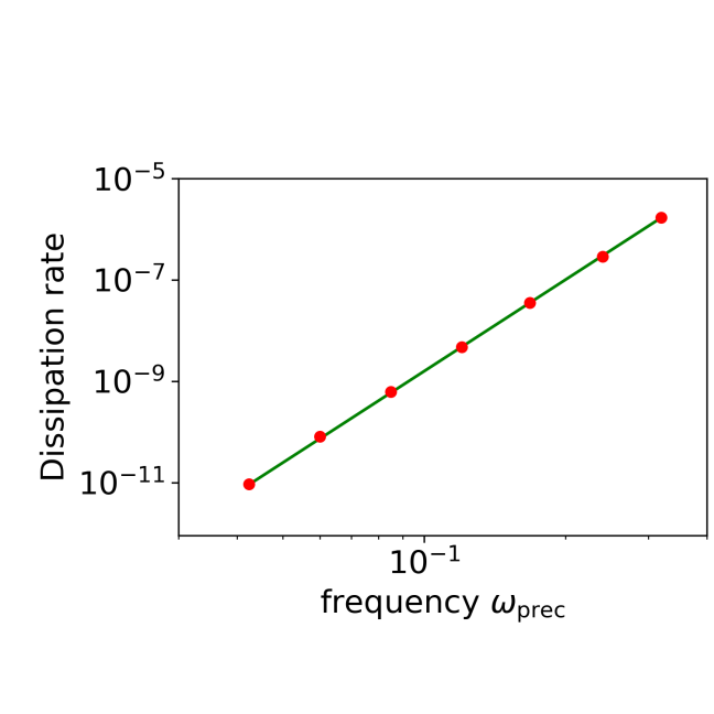
Figure 3: We compare the energy dissipation rates for simulations that are identical except for the amplitude of their initial spin vectors $|{\boldsymbol{\Omega}}_{0}|$. The parameters for these simulations are listed in Tables 2 and Table 4. The $x$ axis is the precession rate $\omega_{\rm prec}$ and the $y$ axis the measured energy dissipation rate. The red points show simulation measurements. The green line has power $P\propto\omega_{\rm prec}^{6}$, predicted for the Kelvin-Voigt model. It was not fit to the points, but was adjusted to intersect the point on the upper right. The dissipation rate is sensitive to spin amplitude and with power that depends on rheology.

Table 4: Oblate ellipsoid simulation parameters for varying spin amplitude

Body shape		Oblate
Axis ratio	$h$	1/3
Spring constant	$k_{s}$	0.08
Shear modulus	$\mu$	$1.5$
Spring damping coefficient	$\gamma_{s}$	4
Viscoelastic relaxation time	$t_{\rm relax}$	0.014
NPA angle	$\theta$	$39.3^{\circ}$
Initial spin $x$ components	${\Omega}_{0x}$	$={\Omega}_{0z}$
Initial spin $y$ component	${\Omega}_{0y}$	0
Initial spin $z$ components	$\Omega_{z0}$	0.4, 0.3, 0.21, 0.15,
"		and 0.106, 0.075, 0.053
Relevant figure		Figure 3

Notes: We carried out a series of simulations with different initial spin values. These simulations are discussed in section 3.2. Additional simulation parameters are listed in Table 2.

3.2 Sensitivity of the energy dissipation rate to spin rate for oblate ellipsoids

Equation 26 gives an expression for the energy dissipation rate for oblate ellipsoids based on that estimated by Frouard & Efroimsky (2018) but modified for a Kelvin-Voigt viscoelastic solid. Using the expression for the precession frequency in equation 13, we can write equation 26 as

$$P^{\rm FE,KV}_{\rm oblate} \approx\frac{a^{7}{\tilde{\omega}}^{6}\rho^{2}\tau_{\rm relax}}{\mu}\frac{(1-h^{2})^{2}}{(1+h^{2})^{2}}\cos^{2}\theta\ \times$$

$$\qquad\left(f^{\rm FE}_{(1)}(h)\sin^{2}\theta\cos^{2}\theta+4f^{\rm FE}_{(2)}(h)\sin^{4}\theta\right).$$ (28)

We estimate that the dissipated power is strongly dependent on the spin rate or $P\propto\tilde{\omega}^{6}$. We can test this by comparing simulations with the same NPA angle $\theta$, shear modulus $\mu$, viscoelastic relaxation time $\tau_{\rm relax}$, and body axis ratio $h$, but different initial $|{\boldsymbol{\Omega}}_{0}|$ spin amplitudes, as $\tilde{\omega}\propto|{\boldsymbol{\Omega}}|\propto\omega_{\rm prec}$ at fixed $\theta$; see equation 13. Figure 3 shows such a series of oblate ellipsoid simulations. The simulation parameters are listed in Tables 2 and 4. We plot as red dots energy dissipation rate measured from the simulations but against the spin precession rate $\omega_{\rm prec}$ which is proportional to $\tilde{\omega}$. We again show a line on the plot that is not fit to the simulation measurements but depends on $\omega_{\rm prec}^{6}$. The line on the figure shows that the energy dissipation rate is consistent with being proportional to $\tilde{\omega}^{6}$ as expected from equation 28.

We find that the Kelvin-Voigt model has power proportional to spin $\tilde{\omega}$ to the sixth power, whereas the Maxwell model has power proportional to the fourth power (equation 19 and that predicted by Frouard & Efroimsky 2018). With a quality factor model, the energy dissipation rate is proportional to the fifth power (equation 81 by Breiter et al. 2012). Wobble damping times are sensitive to rheology.

Table 5: Oblate ellipsoid simulation parameters for varying axis ratio and NPA angle

Body shape		Oblate
Spring constant	$k_{s}$	0.08
Shear modulus	$\mu$	$1.5$
Spring damping coefficients	$\gamma_{s}$	4
Viscoelastic relaxation time	$t_{\rm relax}$	0.014
Frequency	$\tilde{\omega}$	0.5
Axis ratios	$h$	1/3, 1/2, 2/3
NPA angles	$\theta$	10∘ to 80∘ w. increments of 10∘
Axis ratios	$h$	0.1 to 0.9 w. increments of 0.1
NPA angles	$\theta$	$30,45,60^{\circ}$
Relevant figures		Figures 4 and 5

Notes: We carried out two sets of simulations. Each simulations has a different value of $h$ and $\theta$. These simulations are discussed in section 3.3. Initial spin components $\Omega_{x0},\Omega_{0z}$ were computed using equations 14 and 16 from frequency $\tilde{\omega}$ and NPA angle $\theta$. Additional simulation parameters are listed in Table 2.

Table 6: Prolate ellipsoid simulation parameters for varying axis ratio and NPA angle

Body shape		Prolate
Spring constant	$k_{s}$	0.08
Shear modulus	$\mu$	$1.5$
Spring damping coefficients	$\gamma_{s}$	4
Viscoelastic relaxation time	$t_{\rm relax}$	0.014
Frequency	$\tilde{\omega}$	0.5
Axis ratios	$h$	3/2, 2, 3
NPA angle	$\theta$	10∘ to 80∘ w. increments of 10∘
Axis ratios	$h$	1.11, 1.26, 1.50, 1.78, 2.11, 2.51,
"	"	and 2.98, 3.54, 4.21, 5.00
NPA angles	$\theta$	$30,45,60^{\circ}$
Relevant figure		Figure 6

Notes: We carried out two sets of simulations. Simulations have different $h$ and $\theta$. These simulations are discussed in section 3.4. Initial spin components $\Omega_{x0},\Omega_{0z}$ were computed using equations 14 and 16 from frequency $\tilde{\omega}$ and NPA angle $\theta$. Additional simulation parameters are listed in Table 2.

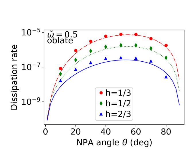
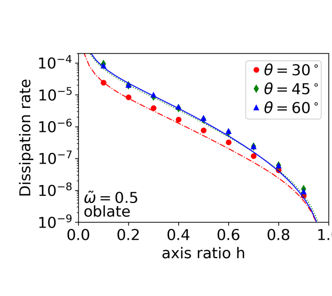
Figure 4: We compare the energy dissipation rates for oblate simulations that are identical except for their body axis ratio and NPA angle $\theta$. The parameters for these simulations are listed in Tables 2 and Table 5. The $x$ axis is the NPA angle $\theta$ and the $y$ axis the measured energy dissipation rate. a) The red circles, green diamonds and blue triangles show measurements from simulations of oblate ellipsoids with axis ratios $h=1/3,1/2,2/3$, respectively. The red dash-dotted, green dotted and blue solid lines lines are computed for the same axis ratios using equation 29 that is based on work by Frouard & Efroimsky (2018). b) Similar to a) except red circles, green diamonds and blue triangles show simulations with NPA angle $\theta=30,45,60^{\circ}$, and the $x$ axis is the axis ratio $h$. The red dash-dotted, green dotted and blue solid lines lines are computed for the same NPA angles using equation 29.

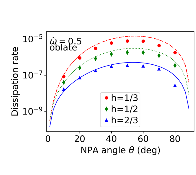
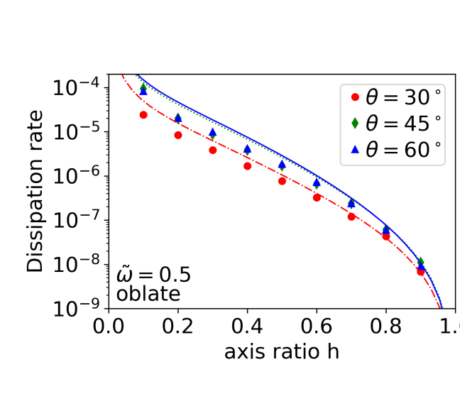
Figure 5: We compare the energy dissipation rates for oblate simulations that are identical except for their body axis ratio and NPA angle $\theta$. These figures are the same as those in Figure 4 except we plot lines computed using equation 35 that are based on calculations by Breiter et al. (2012).

3.3 Sensitivity of dissipation rate to axis ratio and angle for oblates

To explore the sensitivity of the dissipation rate to body axis and spin axis orientation we fix the frequency $\tilde{\omega}$, shear modulus and viscosity but vary the body axis ratio $h$ and NPA angle $\theta$. We ran 3 sets of oblate ellipsoid simulations with body axis ratios $h=1/3,1/2,2/3$. Each set contains 8 simulations with NPA angles $\theta=10,20,30,40,50,60,70$ and $80^{\circ}$. We also ran 3 sets of oblate simulations with $\theta=30,45,60^{\circ}$ and 10 different values of axis ratio $h$. Initial spin vectors for the simulations were set using equations 14 and 16 at $t=0$. Parameters for these simulations are listed in Table 5 and the energy dissipations are plotted in Figures 4 and 5 as a function of NPA angle (top panels) and axis ratios $h$ (bottom panels).

The normalization in equation 19 depends on semi-major axis $a^{7}$. Our simulations work in units of the radius of the volume equivalent sphere, with $V=\frac{4}{3}\pi abc=\frac{4}{3}\pi R_{\rm vol}^{3}$. For an oblate body with semi axes $a=b$, volume equivalent radius $R_{\rm vol}$ and axis ratio $h=c/a$, we find that semi-major axis $a=h^{-\frac{1}{3}}R_{\rm vol}$. Inserting this into equation 28 we find

$$P^{\rm FE,KV}_{\rm oblate} \approx\frac{R_{\rm vol}^{7}\rho^{2}\tau_{\rm relax}{\tilde{\omega}}^{6}}{\mu h^{\frac{7}{3}}}\frac{(1-h^{2})^{2}}{(1+h^{2})^{2}}\cos^{2}\theta\ \times$$

$$\qquad\left(f^{\rm FE}_{(1)}(h)\sin^{2}\theta\cos^{2}\theta+4f^{\rm FE}_{(2)}(h)\sin^{4}\theta\right)$$ (29)

With $\rho,{\tilde{\omega}},\mu,\tau_{\rm relax},R_{\rm vol}$ in our N-body units, power is in units of $e_{\rm grav}t_{\rm grav}^{-1}$.

In Figure 4 we overplot lines given by equation 29 for oblates. To compute these we used the shear viscosity and viscoelastic relaxation time estimated from the code (and with parameters listed in Table 5), $R_{\rm vol}=1$, and a density of $\rho=3/(4\pi)$, consistent with our N-body units. Three lines in the top panel are computed for three axis ratios $h=1/3,1/2$ and 2/3 and shown as red dash-dotted, green dotted and blue solid lines in Figure 4a as a function of NPA angle $\theta$. In Figure 4b three lines are computed for three NPA angles $\theta=30,45,60^{\circ}$ and are shown as red dash-dotted, green dotted and blue solid lines as a function of varying axis ratio $h$. The model lines are a good match to the numerical measurements, without any additional offsets or normalization. This implies that the analytical prediction by Frouard & Efroimsky (2018) for the Maxwell viscoelastic model is robust, even though we have modified it for the Kelvin-Voigt model.

A perfect match between model and numerical measurements is unlikely because the analytical computation ignores bulk viscosity though our simulated viscoelastic material is compressible and has a bulk viscosity. The bulk viscosity is neglected in the model (equation 29) because it is based on calculations by Frouard & Efroimsky (2018) who neglected bulk viscosity. The computations by Sharma et al. (2005), Frouard & Efroimsky (2018) and Breiter et al. (2012) assume a Poisson ratio $1/4$ which is consistent with our simulated elastic material. In the analytical computations displacements and their partial derivatives are assumed to be small. The analytical models by Sharma et al. (2005); Frouard & Efroimsky (2018) (but not Breiter et al. 2012) ignore compression due to self-gravity. Stress due to constant inertial acceleration (non-varying components of the acceleration; see discussion in appendix C by Frouard & Efroimsky 2018) was ignored by Frouard & Efroimsky (2018) but not by Sharma et al. (2005).

With tidal spin down (but undergoing principal axis rotation) we found that analytical predictions lacking bulk viscosity were 30% lower than the numerical measurements (Frouard et al., 2016). A factor of 30% gives $\log_{10}1.3=0.11$ in log space which would look small in Figure 4. Many of the numerical measurements are slightly higher than the predicted values, and this might be due to the neglect of bulk viscosity in the model that is present in the simulated material.

Using a different derivation of the stress tensor, Breiter et al. (2012) derive the energy dissipation rate for both prolate and oblate ellipsoids. For ellipsoids of rotation (prolates and oblates), the NPA angle used by Breiter et al. (2012) (their $\theta_{s}$ defined in their equation 81) is equivalent to our NPA angle $\theta$. Our precession rate $\omega_{\rm prec}$ is equivalent to their fundamental frequency of wobbling (defined in their equation 58). Their frequency $\tilde{\omega}_{s}$ (defined in their equation 52) is equivalent to our $\tilde{\omega}$. The energy dissipation rate for oblates (equations 103,104, 105 by Breiter et al. 2012) can be written as

$$P^{\rm BR}_{\rm oblate} =\frac{a^{7}\rho^{2}\tilde{\omega}^{5}}{\mu Q}\frac{(1-h^{2})}{(1+h^{2})}\cos\theta\ \times$$

$$\ \ \ \ \left(f^{\rm BR}_{(1)}(h)\sin^{2}\theta\cos^{2}\theta+f^{\rm BR}_{(2)}(h)\sin^{4}\theta\right),$$ (30)

with functions

$$f^{\rm BR}_{(1)}(h) =\frac{32\pi}{105}\frac{2h^{5}}{(1+h^{2})^{4}}\frac{26+35h^{2}}{13+20h^{2}}$$ (31)

$$f^{\rm BR}_{(2)}(h) =\frac{32\pi}{105}\frac{h}{(1+h^{2})^{4}}\frac{25+20h^{2}+16h^{4}}{15+10h^{2}+8h^{4}}.$$ (32)

They model the energy dissipation with a constant quality factor $Q$. This effectively gives a frequency dependent viscoelastic relaxation time $\tau_{\rm relax}\approx Q/\omega_{\rm prec}$ or

$$Q=\tau_{\rm relax}\omega_{\rm prec}=\frac{\eta\omega_{\rm prec}}{\mu}.$$ (33)

We can estimate the energy dissipation rate for a Maxwell model using viscosity $\eta=\tau_{\rm relax}\mu$ and giving

$$P^{\rm BR,MW}_{\rm oblate} =\frac{a^{7}\rho^{2}\tilde{\omega}^{4}}{\eta}\left(f^{\rm BR}_{(1)}(h)\sin^{2}\theta\cos^{2}\theta+f^{\rm BR}_{(2)}(h)\sin^{4}\theta\right),$$ (34)

where we have used equation 13 for the precession rate and replaced $Q$ in equation 30 using equation 33. This equation closely resembles equation 19 (based on equation 57 by Frouard & Efroimsky 2018) except the $h$ dependent functions differ. We identify two terms in equation 34, the first likely arises from acceleration terms that have frequency $\omega_{\rm prec}$ and the second from acceleration terms dependent on $2\omega_{\rm prec}$. We estimate the energy dissipation rate for the Kelvin Voigt model as we did in section 3.1 giving

$$P^{\rm BR,KV}_{\rm oblate} =\frac{R_{\rm vol}^{7}\rho^{2}\tau_{\rm relax}\tilde{\omega}^{6}}{\mu h^{\frac{7}{3}}}\frac{(1-h^{2})^{2}}{(1+h^{2})^{2}}\cos^{2}\theta\ \times$$

$$\quad\left(f^{\rm BR}_{(1)}(h)\sin^{2}\theta\cos^{2}\theta+4f^{\rm BR}_{(2)}(h)\sin^{4}\theta\right).$$ (35)

Lines computed using equation 35 are plotted on the dissipation rate measurements for our oblate simulations in Figure 5. The lines are good match to the numerical measurements. However, they lie slightly above the numerical measurements rather than slightly below them as did those by Frouard & Efroimsky (2018). Within a factor of about 20%, the quality factor based dissipation model by Breiter et al. (2012) is consistent our numerical measurements and with the Maxwell model computed by Frouard & Efroimsky (2018) for oblates if we use equation 33 to relate $Q$ to the viscoelastic relaxation time or viscosity.

3.4 Sensitivity of dissipation rate to axis ratio and angle for prolates

Similar sets of simulations as described in section 3.3 were done for prolate ellipsoids instead of oblates. Again we fix frequency $\tilde{\omega}$, shear modulus and viscosity but vary the body axis ratio and initial NPA angle $\theta$. The simulations have parameters listed in Table 6 and Table 2 and the energy dissipation rates for these simulations are shown in Figure 6. We ran 3 sets of prolate ellipsoid simulations with body axis ratios $h=3,2,3/2$ and with NPA angles $\theta=10,20,30,40,50,60,70$ and $80^{\circ}$. We also ran 3 sets of prolates simulations with $\theta=30,45,60^{\circ}$ and with 10 different values of axis ratio $h$.

Following equation 106 by Breiter et al. (2012) for prolates, equations 30 and 34 here can be modified to apply to prolates by replacing $a$ with $c$, and using our convection for prolate axis ratio $h>1$ (note that Breiter et al. 2012 adopted $h<1$ for prolates). For prolates equations 30 and 34 should be proportional to $c^{7}$ rather than $a^{7}$. For a prolate body with semi-axes $b=c$, volume equivalent radius $R_{\rm vol}$ and axis ratio $h=a/c$, we find that $c=h^{-\frac{1}{3}}R_{\rm vol}$. Replacing $a^{7}$ with $c^{7}=R_{\rm vol}^{7}h^{-7/3}$ in equation 34 gives equation 35, unchanged. Equation 35 should apply to both prolates and oblates, with the convention that $h>1$ for prolates and $h<1$ for oblates.

On Figure 6 we plot lines computed using equation 35 (based on the computations by Breiter et al. 2012 but modified for the Kelvin-Voigt model) with our numerical measurements, finding that they closely match our computations.

Frouard & Efroimsky (2018) used the stress tensor computed by Sharma et al. (2005) for homogeneous ellipsoids and so should be valid for both oblate and prolate ellipsoids. However, to apply to prolates, the semi-major axis $a$ in equation 57 by Frouard & Efroimsky 2018, equations 19, 26, and 28 should be replaced by the semi-axis perpendicular to the axis of symmetry (replace $a^{7}$ by $c^{7}$). Replacing $a^{7}$ with $c^{7}=R_{\rm vol}^{7}h^{-7/3}$ in equation 28 gives equation 29, unchanged. Equation 29 should apply to prolates and oblates. Unfortunately equation 29 does not match our numerical measurements, except at $h\sim 1$. The curves are two orders of magnitude higher than our numerical measurements at large $h$ and an order of magnitude higher at $\theta=45^{\circ}$. We have not found errors in the computations by Frouard & Efroimsky (2018), so we suspect that the stress tensor computed by Sharma et al. (2005) is a good approximation only in the limit of $h\la 1$. Both Sharma et al. (2005) and Breiter et al. (2012) assume traction free boundary conditions but their stress tensors differ (see the discussion in section 6 by Breiter et al. 2012).

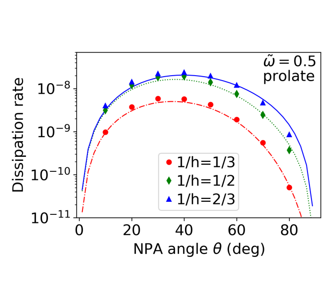
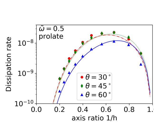
Figure 6: We compare the energy dissipation rates for prolate simulations that are identical except for their body axis ratio and NPA angle $\theta$. Similar to Figure 5 except we show prolate simulations and the $x$ axis is the inverse of $h$. The parameters for these simulations are listed in Tables 2 and Table 6. a) The red circles, green diamonds and blue triangles show measurements for axis ratios $h=3,2,3/2$, respectively. The red dash-dotted, green dotted and blue solid lines lines are computed for the same axis ratios using equation 35 based on work by Breiter et al. (2012). b) The red circles, green diamonds and blue triangles show measurements for NPA angle $\theta=30,45,60^{\circ}$, respectively. The red dash-dotted, green dotted and blue solid lines lines are computed for the same NPA angles using equation 35.

Table 7: Simulations of Inhomogeneous Rotators

Fiducial model
Body shape		Bennu shape model
Spring constant	$k_{s}$	0.32
Shear modulus	$\mu$	$5.2$
Spring damping coefficients	$\gamma_{s}$	4
Viscoelastic relaxation time	$t_{\rm relax}$	$3.8\times 10^{-3}$
Frequency	$\tilde{\omega}$	0.8
NPA angle	$\theta$	50∘
Variants
Core properties	Springs	Viscoelastic parameters
Hard Core	$4k_{s}$, $\gamma_{s}$	$4\mu,\tau_{\rm relax}/4$
Hard Core, similar $\tau_{\rm relax}$	$4k_{s}$, $4\gamma_{s}$	$4\mu,\tau_{\rm relax}$
Soft Core	$k_{s}/4$, $\gamma_{s}$	$\mu/4,4\tau_{\rm relax}$
Soft Core, similar $\tau_{\rm relax}$	$k_{s}/4$, $\gamma_{s}/4$	$\mu/4,\tau_{\rm relax}$
Higher Viscosity Core	$k_{s}$, $4\gamma_{s}$	$\mu,\tau_{\rm relax}/4$
Lower Viscosity Core	$k_{s}$, $\gamma_{s}/4$	$\mu,4\tau_{\rm relax}$
Relevant figure		Figure 7

Additional simulation parameters are listed in Table 2. These simulations are discussed in section 4. The top section of the table lists parameters for a fiducial homogeneous model. We also ran similar simulations with harder and softer cores and cores with higher and lower viscosity. We changed spring constants or/and spring damping parameters only. These variations listed in the second section of the table.

3.5 Discussion on Material properties

As asteroid internal composition and behavior is not well constrained, we take a moment to summarize laboratory estimates for shear modulus $\mu$ and quality factor $Q$ in different materials and touch on estimates for $\mu Q$ in asteroids. The wobble damping timescale is shorter for faster rotators, so more slowly rotating objects can persist in an NPA state for a longer time. The division between NPA and principal axis (PA) rotators in the Asteroid Light Curve Database as a function of asteroid size and rotation period (see Figure 8 by Pravec et al. 2014) is used to estimate $\mu Q$ in asteroid material (building upon Harris 1994). Updated wobble damping timescales estimated by Pravec et al. (2014) from the division are 7-9 times shorter than those estimated by Harris (1994), giving a somewhat lower rough estimate for $\mu Q\sim 10^{11}$ Pa, compared to the $5\times 10^{11}$ Pa estimated by Harris (1994). These estimates for $\mu Q$ can be substantially higher (by about two orders of magnitude) than estimated from tidal dissipation in binary asteroids (e.g., Taylor & Margot 2011; Nimmo & Matsuyama 2017). It might be difficult to resolve this quantitative disagreement without better understanding of spin excitation, YORP, binary-YORP and binary formation and evolutionary processes.

To put things in context with stress/strains measured in laboratory experiments, we roughly estimate the sizes of stress and strain rates for asteroids undergoing NPA rotation,

$$\sigma \sim\rho\Omega^{2}R^{2}$$

$$=5\ {\rm Pa}\left(\frac{\rho}{1000\ {\rm kg~{}m}^{3}}\right)\left(\frac{1\ {\rm day}}{P}\right)^{2}\left(\frac{R}{1\ {\rm km}}\right)^{2}$$ (36)

where $P=2\pi/\Omega$. The strain and strain rate

$$\epsilon \sim\frac{\sigma}{\mu}$$

$$\sim 5\times 10^{-9}\left(\frac{\rho}{1000\ {\rm kg~{}m}^{3}}\right)\left(\frac{1\ {\rm day}}{P}\right)^{2}\left(\frac{R}{1\ {\rm km}}\right)^{2}\left(\frac{1\ {\rm GPa}}{\mu}\right)$$

$$\dot{\epsilon} \sim\epsilon\Omega$$ (37)

$$\sim 4\times 10^{-13}{\rm s}^{-1}\left(\frac{\rho}{1000\ {\rm kg~{}m}^{3}}\right)\left(\frac{1\ {\rm day}}{P}\right)^{3}\left(\frac{R}{1\ {\rm km}}\right)^{2}\left(\frac{1\ {\rm GPa}}{\mu}\right).$$ (38)

To be more accurate, the sensitivity to spin state and body axis ratios needs to be taken into account. These values illustrate that oscillating stress, strain and strain rate during NPA rotation are quite low compared to laboratory experimental values that tend to have $\dot{\epsilon}\ga 10^{-12}{\rm s}^{-1},\sigma\ga 10^{3}$ Pa (e.g., Goldsby & Kohlstedt 2001; McCarthy & Cooper 2016).

Mechanisms for dissipation caused by constant stress and causing creep may differ from those caused by periodic stress/strain cycling (e.g., Cooper 2002; McCarthy & Cooper 2016). Quality factor and shear modulus for different materials are likely dependent on amplitude as well as frequency. The wobble damping regime is low stress and strain rate and low frequency compared to seismic frequencies, and not necessarily similar to that for static stress. Most laboratory studies find that $Q$ increases slowly as frequency increases, with a power law, $Q\propto f^{\alpha}$ and exponent $\alpha$ in the range 0.1–0.4 (e.g., Cooper 2002; McCarthy & Cooper 2016). Equation 33 gives viscosity $\eta=\mu Q/\omega_{\rm prec}$, so a weak power law $Q$ dependency on frequency partly cancels the frequency dependence of the viscosity, at a fixed shear modulus. Using a spin period of 10 days and its associated frequency, the viscosity $\eta\sim 1.4\times 10^{16}$ Pa s for $\mu Q=10^{11}$ Pa.

For ’warm’ ice at temperature $\sim 240$ K, laboratory experiments of low-frequency, small-strain periodic loading at Europa’s orbital or tidal flexing frequency, $f\sim 2\times 10^{-5}$ Hz, (corresponding to a rotation period of 3.55 days) give an attenuation coefficient in the range $Q\sim$ 10 – 100 (McCarthy & Cooper, 2016). The physical mechanism is chemical diffusion on grain boundaries or strain accommodated intracrystalline dislocation slip. With a Young’s modulus of a few GPa, (and shear modulus about half this), the product $\mu Q$ for warm ice is similar to that estimated by Harris (1994) and Pravec et al. (2014). Viscosity for colder ice would be a few orders of magnitude lower, so icy bodies in the outer solar system might take longer to damp into principal axis rotation states.

However, ice fractions could be low for many asteroids. The Young’s modulus for solid rocky materials is about 50 GPa and the $Q$ value at the same frequency regime for polycrystalline silicates may be similar to that of ice (Jackson et al., 2002). The estimated $\mu Q\sim 10^{11}$ Pa would require a lower $Q\sim 10$ value to be consistent with the NPA/PA division if asteroids are solid rock.

The Young’s modulus of a porous rubble pile or a granular material can be an order of magnitude lower than that of its grains (see http://www.geotechdata.info/, Goldreich & Sari 2009). Hydrostatic pressure, due to self-gravity, creates force chains through the medium, comprised of forces exerted at particle-particle contacts. At low porosity, contacts can flex, and the granular medium can be softer than the individual particles themselves. The medium need not have tensile strength to exhibit viscoelastic relaxation when existing force chains are periodically varied at low amplitude. Laboratory granular media can have high attenuation rates, $Q\sim 10$, for seismic waves (e.g., as does dry sand and silt; Oelze et al. 2002), though lunar regolith has low seismic attenuation (Dainty et al., 1974; Toksöz et al., 1974; Nakamura, 1976), with $Q\sim 3000$. The lower the porosity and coarser the granular medium (having larger grains), the more it behaves like a solid. The material strength could also depend on static hydrostatic pressure and consequently on the size of the asteroid. If the Young’s modulus is similar to that of ice or a few GPa, (and about a factor of 10 lower than that of solid rocky materials) then $Q\sim 100$ would match the estimate for $\mu Q\sim 10^{11}$ Pa based on asteroid light curves. The estimate for $\mu Q$ by Pravec et al. (2014) lies easily within the large uncertainties if most asteroids are dry granular rocky materials.

The division between NPA and principal axis rotators in the Light Curve Database is better matched by a line of constant wobble damping time and does not follow the collisional lifetime or YORP time scale (Pravec et al., 2014) so the excitation mechanism has not been pinned down. Pravec et al. (2014) suggested that this trend could be explained if $\mu Q$ depends on asteroid size, decreasing for smaller asteroids. This can arise if larger asteroid cores contain lower porosity cores. A larger ice core fraction would make the core weaker but possibly more dissipative. Stress, strain and strain rate (equations 36, 37, 38) all depend on asteroid size and all are larger for larger asteroids. If the dissipation rate is higher (giving a lower $Q$) at larger stress, strain and strain rate, then $\mu Q$ could be lower for larger asteroids, opposite to the expected trend.

Pravec et al. (2014) adopted the quality factor ($Q$) based model for the wobble damping time (Sharma et al., 2005; Breiter et al., 2012) and giving a damping time that is proportional to the spin frequency to the minus third power, as in equation 1; $\tau\propto\mu Q/(\rho R^{2}\tilde{\omega}^{3})$ (also see equation 3 by Pravec et al. 2014). Because the energy dissipation rate for the Maxwell model depends on viscosity rater than $Q$, a constant viscosity model gives lifetime for NPA rotation of $\tau\propto\eta/(\rho R^{2}\tilde{\omega}^{2})$ (Frouard & Efroimsky, 2018). The use of a constant viscosity $\eta$ rather than constant quality factor $Q$ model changes the relation between size and spin frequency at a constant wobble damping lifetime and so would affect the slope of the NPA/PA division on a plot of size versus spin frequency. At a constant wobble damping time $R\propto\tilde{\omega}^{-\frac{3}{2}}$ for the constant $Q$ based estimates, but $R\propto\tilde{\omega}^{-1}$ for the constant viscosity and Maxwell based estimate. The Maxwell model by Frouard & Efroimsky (2018) slightly alleviates, but does not remove altogether, the tension between the distribution of NPA rotators as a function of size and spin rate, and that expected if they all have the same material properties (and if NPA rotation is exited by collisions).

For ellipsoids with rotational symmetry, a Fourier expansion of the stress and strain contain only two frequencies, the precession frequency and twice this frequency. For triaxial bodies, the expansion contains higher frequencies. Since most materials show higher viscoelastic dissipation rates at higher frequencies, frequency sensitive viscoelastic wobble damping models would predict more rapid damping for elongated bodies than for more nearly spherical ones. Future and larger light curve databases might be used to reexamine the question of how asteroid tumbling is excited and damped and how the dissipation in asteroid material depends on frequency.

The YORP effect acts adiabatically so would not be expected to excite NPA rotation. However, if a body is disrupted when spun up by YORP (e.g., Sánchez & Scheeres 2018) then landslides and equatorial mass shedding might excite tumbling. In this paper we have computed energy dissipation rates and have not integrated them to estimate wobble damping times. This integration is done assuming that angular momentum is conserved (Sharma et al., 2005; Breiter et al., 2012; Frouard & Efroimsky, 2018). However YORP effect induced spin variations would violate that conservation law. There is a non-trivial connection between YORP, composition and rotation state (e.g., see Breiter & Murawiecka 2015).

4 Inhomogeneous Rotators

In this section we measure the energy dissipation rate for nearly spherical wobbling bodies with hard and soft cores. Inspired by the recent arrival of the OSIRIS-REx spacecraft at asteroid 101955 Bennu in Nov. 2018, we explore wobble damping using the radar based shape mode by Nolan et al. (2013), as when studying elastic response to impacts (Quillen et al., 2019b). We are interested in the sensitivity of the wobble damping time to variations in internal composition. The initial node distribution and spring network are created in the same way as for the ellipsoids, except we retain randomly generated particles within the shape model; for more information see Quillen et al. (2019b). This shape is nearly spherical, with moment of inertia ratios $\sqrt{I_{1}/I_{3}}\sim 0.94$ and $\sqrt{I_{1}/I_{2}}\sim 0.98$. Here $I_{1}<I_{2}<I_{3}$ are the three moments of inertia we measured numerically from our simulated mass node distribution.

We compared the energy dissipation rate for the Bennu shape model with a triaxial ellipsoid model with similar moments of inertia and initial spin values, $\tilde{\omega}\sim 0.6$, and NPA angle $\theta\sim 50^{\circ}$ (we computed the angle between the initial spin vector and angular momentum). As the body is nearly oblate, the angle does not exhibit large variations during the simulation. Comparing a homogeneous Bennu shape model with the similar triaxial ellipsoid, the numerically measured energy dissipation rates differed by less than 15%. We conclude that shape variations for near spherical homogenous bodies do not strongly affect the energy dissipation rate during wobbling damping.

To probe the sensitivity of the wobble damping time to internal composition, we varied the properties of core springs, leaving springs nearer the surface unchanged. For these simulations we use the Bennu shape model, starting with a fiducial and homogeneous model parameters with parameters listed in the top of Table 7. We varied 20%, 50% or 80% of the springs, changing their spring constants $k_{s}$, damping parameter $\gamma_{s}$ or both parameters. We chose springs to change based on their midpoint positions. For the 20%, 50% and 80% core models we varied springs with midpoints within a radius of 0.60, 0.78, and 0.92, respectively, of the center of the body, giving harder or softer or more less viscous cores compared to the fiducial model. The types of spring variations are listed in the bottom of Table 7. For hard and soft core simulations we multiplied the fiducial model spring constant by 4 or 1/4. For higher viscosity and lower viscosity simulations we multiplied the spring damping parameter by 4 or 1/4. We also multiplied both spring constant and damping parameter by the same factors to carry out simulations of hard and soft cores that have the same viscoelastic relaxation time as their shells.

Energy dissipation rates for the hard and soft core models are shown in Figure 7, normalized to the dissipation rate measured for the homogeneous and fiducial model (shown as a large blue dot on the left). As the energy dissipation rate is proportional to $\tau_{\rm relax}/\mu$ (as in equation 35), the homogeneous models with all springs changed should have energy dissipation rates 4 or 16 times larger or smaller than the fiducial model. Points on the right hand side of Figure 7 are these factors of the homogeneous or fiducial model. Figure 7 shows that the energy dissipation rate from wobble damping is not linearly dependent upon the core volume. The energy dissipation rate for wobble damping is more sensitive to the core material properties than those in the shell. It is well known that viscoelastic tidal heating is stronger at the base of a solid but dissipative shell (e.g., Beuthe 2013), so we should not be surprised that the energy dissipation rate for bodies undergoing NPA rotation is more strongly influenced by material properties in the core than near the surface.

The stress and strain tensors computed by Sharma et al. (2005); Breiter et al. (2012) are quadratic in coordinates but also include constant terms. The terms that are quadratic in coordinates drop to zero in the core leaving the constant term setting the core stress and strain. We consider two simple models for the sensitivity of the energy dissipation rate to modified core properties. We consider stress quadratically dependent on a single direction (the z-model)

$$\sigma \propto(1-z^{2})$$ (39)

here aligned with the $z$ axis, or quadratically dependent on the radius (the r-model)

$$\sigma \propto(1-r^{2}).$$ (40)

Both models are traction free on the surface with $r=1$. The actual stress tensors contain numerous quadratic terms (see the appendices by Sharma et al. 2005; Breiter et al. 2012). We assume a energy dissipation rate per unit volume $p\propto\frac{\tau_{\rm relax}}{\mu}\sigma^{2}$ and integrate over the volume of a sphere to find the total dissipation rate. We assume a spherical boundary between core and shell with a core that has a viscoelastic relaxation time $\tau_{\rm relax,core}$ and shear modulus $\mu_{\rm core}$ and a shell that has $\tau_{\rm relax,fid}$ and $\mu_{\rm fid}$. The ratio of dissipation rates of the model with core compared to fiducial model (computed by integrating over volume) as a function of the fraction of volume in the core $f$

$$\frac{P(f)}{P_{\rm fiducial}}=\left(\frac{\tau_{\rm relax,core}}{\tau_{\rm relax,fid}}\frac{\mu_{\rm fid}}{\mu_{\rm core}}-1\right)\frac{f\left(1+a_{2}f^{\frac{2}{3}}+a_{4}f^{\frac{4}{3}}\right)}{\left(1+a_{2}+a_{4}\right)}+1,$$ (41)

with coefficients

$$a_{2}=-\frac{2}{5} \qquad a_{4}=\frac{3}{35} {\rm z-model},$$ (42)

$$a_{2}=-\frac{6}{5} \qquad a_{4}=\frac{3}{7} {\rm r-model}.$$ (43)

In Figure 7 we have plotted equation 41 for the z-model with dotted lines for the soft core simulations. These have $\tau_{\rm relax,core}/\mu_{\rm core}=$ 4 or 16 times that of the fiducial model. We plotted the r-model with dot dashed lines and with $\tau_{\rm relax,core}/\mu_{\rm core}=$ 1/4 or 1/16 for the hard core models. The z-model is a pretty good match to soft core simulations and the r-model is a pretty good match to hard core simulations. We lack a qualitative understanding on why a single quadratic stress model failed to cover both settings. Until analytical models are extended to cover core/shell models, these rough models can be used to estimate wobble damping times in nearly spherical asteroids such as Bennu, but with core material properties differing from those near the surface.

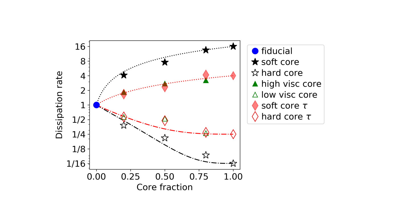
Figure 7: Energy dissipation rates for simulations of core/shell inhomogeneous bodies based on the Bennu shape model. The $y$ axis shows the the energy dissipation rates normalized to the homogeneous or fiducial simulation and with a log scale. The $x$ axis gives the fraction of springs that are varied. The homogenous fiducial simulation is shown as a blue circle and has parameters listed in the top of Table 7. Harder cores have solid or filled point types and softer cores have non-filled point types. The types of cores are labelled in the key and refer to the descriptions in the bottom half of Table 7. The dotted lines show z-models and the dot-dashed lines show r-models computed with equation 41 that are based on quadratic models for internal stress.

5 Summary and Discussion

In this paper we have carried out numerical simulations of homogenous oblate and prolate ellipsoids in NPA rotation states. We have used a mass-spring N-body code, approximating a Kelvin-Voigt viscoelastic material, to measure the rate of energy dissipation of ellipsoids undergoing NPA rotation. By independently varying the spin rate, while keeping axis ratios, shear modulus, viscoelastic relaxation time and spin orientation fixed, we measured how the energy dissipation rate depends on spin. We find that the dissipation rate is sensitive to spin to the 6-th power for the Kelvin-Voigt rheology rather than 4-th power as is true in the Maxwell rheology (Frouard & Efroimsky, 2018) or 5-th power as for the quality factor $Q$ based estimates (Breiter et al., 2012). The sensitivity of the energy dissipation rate to rheology suggests that tumbling damping times are sensitive to the material properties of asteroids, and as a consequence the statistics of their spin states could be sensitive to their material properties, and as suggested by Pravec et al. (2014).

By independently varying the spring damping rate, while keeping shear modulus, axis ratios, and initial spin vector fixed, we found how the energy dissipation rate depends on viscoelastic relaxation time and precession frequency. The sensitivity of the dissipation rate to viscoelastic relaxation time (set by the spring damping) allowed us to directly compare our dissipation rates to those predicted for a Maxwell rheology (Frouard & Efroimsky, 2018).

Our numerically measured values of energy dissipation for oblates range over more than 4 orders of magnitude and match the analytical predictions by Frouard & Efroimsky (2018) as a function of NPA angle and axis ratio after they have been modified for the Kelvin-Voigt rheology. They also match the quality factor based computations by Breiter et al. (2012) after modification. The match is quite good even though bulk viscosity and gravitational compression are neglected in the analytical calculations and both are present in the numerical simulations. In our study of tidal spin down (Frouard et al., 2016), we suspect that our neglect of bulk viscosity in the analytical calculation gave a 30% discrepancy between predicted and measured spin down rates. Because the energy dissipation rate due to NPA rotation varies over many orders of magnitude, a 30% discrepancy would seem small on our plots. Our numerical measurements tend to be slightly higher than the predicted values by Frouard & Efroimsky (2018) and this could be in part due to the neglect of bulk viscosity in the analytical model. In contrast, the predicted values by Breiter et al. (2012) give slightly higher dissipation rates than we measure numerically. The discrepancies between models and simulations are at the level of about 20%, underscoring the remarkable accuracy of both analytical and numerical computations.

We carried out a similar series of simulations of prolate ellipsoids, finding that the $Q$ based model by Breiter et al. (2012) gives a good match to our numerical measurements. Our success in comparing numerical results and theoretical results based on different linear rheologies motivated us to reexamine and discuss estimates for the shear modulus and quality factor of asteroid material. We primarily did this to highlight the uncertainties in material properties of asteroids and because the recent analytical works (Breiter et al., 2012; Frouard & Efroimsky, 2018) had not touched on recent laboratory measurements of $Q$ and elastic modulus.

In section 4 we carried out a short numerical exploration of the energy dissipation rate of nearly spherical wobbling bodies with hard and soft cores. We found that the energy dissipation rate for wobble damping is more sensitive to the core material properties than those in the shell. We found that an quadratic internal stress models (see the appendices by Sharma et al. 2005; Breiter et al. 2012) matched the numerically measured energy dissipation rates as a function of core volume, though the form of the model differed between the hard core and soft core simulations.

We also explored (but do not discuss) long simulations of elongated but weak bodies following the progress of a single body as it relaxed to principal axis rotation. Occasionally we saw time periods with rapid energy dissipation. We attribute this to normal mode excitation, occurring when a spin frequency matches a bending mode. We have not focused on this phenomena here as it happens only in a soft body regime where the normal mode frequencies are close to the precession frequency and asteroids tend to be too stiff to be in this regime. However, we do want to bring it to the attention of the reader as this capability of a mass-spring model code might prove useful in the future. Normal mode excitation would be necessarily ignored in most analytical computations of wobble damping and did not occur during the short simulations carried out in this paper, but can seen in our simulations when excited by an impact (e.g., Quillen et al. 2019b).

In this study we have primarily restricted our simulations to ellipsoids with rotational symmetry. For triaxial bodies, the acceleration in the body frame contains more than two frequency components. This makes it more challenging to relate the numerically estimated energy dissipation rates to those of the Maxwell or $Q$ based wobble damping models. This motivates future development of more sophisticated numerical techniques to go beyond the mass spring model used here that approximates a Kelvin-Voigt model. Wobble damping in triaxial bodies is complicated by the transition between short axis and long axis rotation modes. Even an infinitesimally small triaxiality from a prolate shape alters the relaxational dynamics, owing to the emergence of a long period separatrix dividing the initial body’s trajectories from the lowest energy end-state. Near the separatrix the tumbling-relaxation process slows considerably (Efroimsky, 2001, 2002). This makes future of study of triaxial bodies undergoing NPA rotation particularly interesting.

Acknowledgements:

We thank Julien Frouard and Michael Efroimsky for helpful, constructive suggestions and comments that have corrected and improved this manuscript. We thank Eric Blackman, Esteban Wright, Larkin Martini and Randal Nelson for helpful discussions.

This material is based upon work supported in part supported by NASA grant 80NSSC17K0771, and National Science Foundation Grant No. PHY-1757062.

Code used in this paper is available at https://github.com/aquillen/wobble .

References

- Belton et al. (1991) Belton M. J., Julian W. H., Anderson A. J., Mueller B. E., 1991, Icarus, 93, 183
- Belton et al. (2018) Belton M. J. S., et al., 2018, The Astrophysical Journal, 856, L21
- Beuthe (2013) Beuthe M., 2013, Icarus, 223, 308
- Breiter & Murawiecka (2015) Breiter S., Murawiecka M., 2015, Monthly Notices of the Royal Astronomical Society, 449, 2489
- Breiter et al. (2012) Breiter S., Rozek A., Vokrouhlicky D., 2012, Monthly Notices Royal Astronomical Society, 427, 755
- Burns & Safronov (1973) Burns J. A., Safronov V. S., 1973, Monthly Notices Royal Astronomical Society, 165, 403
- Celletti (2010) Celletti A., 2010, Stability and Chaos in Celestial Mechanics. Praxis Publishing Ltd, Chichester, UK
- Chang et al. (2017) Chang C.-K., Lin H.-W., Ip W.-H., Prince T. A., Kulkarni S. R., Levitan D., Laher R., Surace J., 2017, Geoscience Letters, 4, 17
- Cooper (2002) Cooper R., 2002, Reviews in Mineralogy and Geochemistry Mineral. Geochem., 51, 253
- Dainty et al. (1974) Dainty A., Toksöz M. N., Anderson K., Pines P., Nakamura Y., Latham G., 1974, Moon, 9, 11
- Drahus et al. (2018) Drahus M., Guzik P., Waniak W., Handzlik B., Kurowski S., Xu S., 2018, Nature Astronomy, 2, 407
- Efroimsky (2001) Efroimsky M., 2001, Planetary and Space Science, 49, 937
- Efroimsky (2002) Efroimsky M., 2002, Advances in Space Research, 29, 725
- Efroimsky & Lazarian (2000) Efroimsky M., Lazarian A., 2000, Monthly Notices Royal Astronomical Society, 311, 269
- Fraser et al. (2018) Fraser W. C., Pravec P., Fitzsimmons A., Lacerda P., Bannister M. T., Snodgrass C., Smolić I., 2018, Nature Astronomy, 2, 383