Sheaves: A Topological Approach to Big Data

Abstract

This document develops general concepts useful for extracting knowledge embedded in large graphs or datasets that have pair-wise relationships, such as cause-effect-type relations. Almost no underlying assumptions are made, other than that the data can be presented in terms of pair-wise relationships between objects/events. This assumption is used to mine for patterns in the dataset, defining a reduced graph or dataset that boils-down or concentrates information into a more compact form. The resulting extracted structure or set of patterns are manifestly symbolic in nature, as they capture and encode the graph structure of the dataset in terms of a (generative) grammar. This structure is identified as having the formal mathematical structure of a sheaf. In essence, this paper introduces the basic concepts of sheaf theory into the domain of graphical datasets.

DRAFT: This is an unfinished draft; the last 1/4th of the document needs a complete make-over.

^*Hanson Robotics; SingularityNET; <linasvepstas@gmail.com>

ACM Subject Classification:
• Theory of computation—Models of computation;500,
• Theory of computation—Formal languages and automata theory—Grammars and context-free languages;500,
• Theory of computation—Design and analysis of algorithms—Graph algorithms analysis;500

Intro

This document presents some definitions and vocabulary for working with datasets that contain complex relationships, applicable to a large variety of application domains. The concepts borrow from graph theory, and several other areas of mathematics. The goal is to define a way of thinking about complex graphs, and how they can be simplified and condensed into simpler graphs that “concentrate” embedded knowledge into a more manageable size. The output of the process is a grammar that summarizes or captures the significant or important relationships.

The ideas described here are not terribly complex; they represent a kind-of “folk knowledge” generally known to a number of practitioners. However, I am not currently aware of any kind of presentation of this information, either in review/summary form, or as a fully articulated book or text. The background knowledge appears to be scattered across wide domains, and occur primarily in highly abstract settings, outside of the mainstream computer-science and data-analysis domain. Thus, this document tries to provide an introduction to these concepts in a plain-spoken language. The hope is to be precise enough that there will be few complaints from the mathematically rigorous-minded, yet simple enough that “anyone” can follow through and understand.

Some examples are provided, primarily drawn from linguistics. However, the concepts are generally applicable, and should prove useful for analyzing any kind of dataset expressed with pair-wise relationships, but containing hidden (non-obvious) complex cause-and-effect relationships. Such datasets include genomic and proteomic data, social-graph data, and even such social policy information.

Consider the example of determining the effectiveness of educational curricula. When teaching students, one never teaches advanced topics until foundations are laid. Yet many students struggle. Given raw data on a large sample of students, and the curricula they were subjected to, can one discern sequences and dependencies of cause-and-effect in this data? Can one find the most effective curriculum to teach, that advances the greatest number of students? Can one discover different classes of students, some who respond better to one style than another? My belief is that these questions can not only be answered, but that the framework described here can be used to uncover this structure.

Another example might be the analysis of motives and actions in humans. This includes analysis from real life, as well as the narratives of books and movies. In a book setting, the author cannot easily put characters into action until some basic sketch of personality and motives is developed. Motives can’t be understood until a setting is established. If one can break down a large number of books/movies into pairs of related facts/scenes/remarks/actions, one can then extract a grammar of relationships, to see exactly what is involved in the movement of a narrative from here to there.

Much of this document is devoted to stating definitions for a few key structures used to talk about the general problem of discerning relationships and structure. The definitions are inspired by and draw upon concepts from algebraic topology, but mostly avoid both the rigor and the difficulty of that topic.

The definitions provide a framework, rather than an algorithm. It is up to the user to provide some mechanism for judging similarity - and this can be anything: some neural net, Bayesian net, Markov chain, or some vector space or SVM-style technique; the overall framework is agnostic as to these details. The goal is to provide a way of talking about, thinking about and presenting data so that the important knowledge contained in it is captured and described, boiled down to a manageable, workable state from a large raw dump of pair-relationship data.

Currently, the ideas described here are employed in a machine-learning project that attempts to extract the structure of natural language in an unsupervised way. Thus, the primary, detailed examples will come from the natural language domain. The theory should be far more general than that.

This document resides in, accompanies source code that implements the ideas here. Specifically, it is in https://github.com/opencog/atomspace/tree/master/opencog/sheafhttps://github.com/opencog/atomspace/tree/master/opencog/sheaf and it spills over into other files, such as https://github.com/opencog/opencog/blob/master/opencog/nlp/learn/scm/gram-class.scmhttps://github.com/opencog/opencog/blob/master/ opencog/nlp/learn/scm/gram-class.scm This code is in active development, and is likely to have changed by a lot since this was written. This document is not intended to describe the code; rather, it is meant to describe the general underlying concepts.

For the mathematically inclined, please be aware that the concepts described here touch on the tiniest tips of some very deep mathematical icebergs, specifically in parsing, type theory and category theory. I have no hope of providing the needed background, as these fields are sophisticated and immense. The reader is encouraged to study these on their own, especially as they are applied in computer science and linguistics. There are many good texts on these topics.

This document is organized as follows. The first part of provides a definition of a “section” of a graph. A section is a lot like a subgraph, except that it explicitly indicates which edges were cut to form the subgraph. The next part defines and articulates the concept of projection, and shows how it can be used to form quotients. The quotients or projections are termed “stalks”, and, because each stalk comes festooned with connectors, they can be thought to resemble corn-stalks. The next part shows how stalks can be tied together to form sheaves, and reviews the axioms of sheaf theory to show that this name is appropriate.

After this comes a lighting review of how data mining, pattern mining and clustering can be viewed in the context of sheaves. After this come two asides: a quick sketch of type theory, illustrating the interplay between data-mined patterns and the concept of types. Another aside reviews the nature of parsing, illustrating that parsing algorithms implement the gluing axiom of sheaves, viz, that gluing and parsing are the same thing. The final part examines polymorphic behavior. Polymoprhism is that point where syntax begins to touch semantics, where deep structure becomes distinguished from surface structure.

Sections

Begin with the standard definition of a graph.

Definition.

A graph $G=\left(V,E\right)$ is an ordered pair $\left(V,E\right)$ of two sets, the first being the set $V$ of vertices, and the second being the set $E$ of edges. An edge $e\in E$ is a pair $\left(v_{1},v_{2}\right)$ of vertices, where every $v_{k}$ must be a member of $V$. That is, edges in $E$ can only connect vertexes in $V$, and not to something else. $\diamond$

For directed graphs, the vertex ordering in the edge matters. For undirected graphs, it does not. The subsequent will mostly leave this distinction unspecified, and allow either (or both) directed and undirected edges, as the occasion and the need fits. Distinguishing between directed and undirected graphs is not important, at this point. In most of what follows, it will usually be assumed that there are no edges with $v_{1}=v_{2}$ (loops that connect back to themselves) and that there is at most one edge connecting any given pair of vertexes. These assumptions are being made to simplify the discussion; they are not meant to be a fundamental limitation. It just makes things easier to talk about and less cluttered at the start. The primary application does not require either construct, and it is straight-forward to add extensions to provide these features. Similar remarks apply to graphs with labeled vertexes or edges (such as “colored” edges, vertexes or edges with numerical weights on them, etc). Just keep in mind that such additional markup may appear out of thin air, later on.

Besides the above definition, there are other ways of defining and specifying graphs. The one that will be of primary interest here will be one that defines graphs as a collection of sections. These, in turn, are composed of seeds.

Definition.

A seed is a vertex and the set of edges that connect to it. That is, it is the pair $\left(v,E_{v}\right)$ where $v$ is a single vertex, and $E_{v}$ is a set of edges containing that vertex, i.e. that set of edges having $v$ as one or the other endpoint. The vertex $v$ may be called the germ of the seed. For each edge in the edge set, the other vertex is called the connector.$\diamond$

It should be clear that, given a graph $G$, one can equivalently describe it as a set of seeds (one simply lists all of the vertexes, and all of the edges attached to each vertex). The converse is not “naturally” true. Consider a single seed, consisting of one vertex $v_{1}$, and a single edge $e=\left(v_{1},v_{2}\right)$. Then the pair $\left(V,E\right)$ with $V=\left\{v_{1}\right\}$ and $E=\left\{\left(v_{1},v_{2}\right)\right\}$ is not a graph, because $v_{2}$ is missing from the set $V$. Of course, we could implicitly include $v_{2}$ in the collection of vertexes, but this is not “natural”, if one is taking the germs of the seeds to define the vertexes of the graph.

Thus, given a seed, each edge in that seed has one “connected” endpoint, and one “unconnected” endpoint. The “connected” endpoint is that endpoint that is $v$. The other endpoint will commonly be called the connector; equivalently, the edge can be taken to be the connector. Perhaps it should be called a half-edge, as one end-point is specified, but missing.

The seed can be visualized as a ball, with a bunch of sticks sticking out of it. A burr one might collect on one’s clothing. One can envision a seed as an analog of an open set in topology: the center (the germ) is part of the set, and then there’s some more, but the boundary is not part of the set. The vertexes on the unconnected ends of the edges are not a part of the seed.

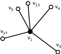
Figure 0.1: A seed

Just as one can cover a topological space with a collection of open sets, so one can also cover a graph with seeds. This analogy is firm: if one has open sets $U_{i}$ and $U_{j}$ and $U_{i}\cap U_{j}\neq\emptyset$ then one can take $U_{i}$ and $U_{j}$ to be vertices, and $U_{i}\cap U_{j}$ to be an edge running between them.

More definitions are needed to advance the ideas of connecting and covering.

Definition.

A section is a set of seeds. $\diamond$

It should be clear that a graph $G$ can be expressed as section; that section has the nice property that all of the germs appear once (and only once) in the set $V$ of $G$, and that all of the edges in $E$ appear twice, once each in two distinct seeds. This connectivity property motivates the following definition:

Definition.

Given a section $S$, a link is any edge $\left(v_{1},v_{2}\right)$ where both $v_{1}$ and $v_{2}$ appear as germs of seeds in $S$. Two seeds are connected when there is a link between them. $\diamond$

This definition of a link is imprecise. A more proper, technical definition is that a link can be formed only when the germ $v_{1}$ has $v_{2}$ as a connector, and also, at the same time, the germ $v_{2}$ has $v_{1}$ as a connector; only then can the two be joined together. The joining is meant to be optional, not mandatory: just because a section contains connectors that can be joined, it does not imply that they must be. The joining is also meant to consume the connectors as a resource: once two connectors have been connected, neither one is free to make connections elsewhere.

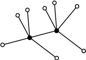
Figure 0.2: Two linked (connected) seeds

The use of links allows the concepts of paths and connectivity, taken from graph theory, to be imported into the current context. Thus, one can obviously define:

Definition.

A connected section, or a contiguous section is a section where every germ is connected to every other germ via a path through the edges. $\diamond$

In graph theory, this would normally be called a “connected graph”, but we cannot fairly call it that because the seeds and sections were defined in such a way that they are not graphs; they only become graphs when they are fully connected. Never-the-less, it is fairly safe and straight-forward to apply common concepts from graph-theory. Sections are almost like graphs, but not quite.

Note that there are two types of edges in a section: those edges that connect to nothing, and those edges that connect to other seeds in that section. Henceforth, the unconnected edges will be called connectors (as defined above), while the fully-connected edges will be called links (also defined above). Connectors can be thought of as a kind-of half-edge: incomplete, missing the far end, while links are fully connected, whole.

Seeds and sections can (and should!) be visualized as hedgehogs - a body with spines sticking out of it - the connectors can be thought of as the spiny bits sticking out, waiting to make a connection, while the hedgehog body is that collection of vertices and the fully-connected links between them.

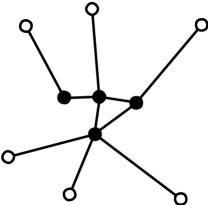
Figure 0.3: A connected section

Implicit in the above definitions was that, during link formation, an edge is only allowed to connect to another seed if and only if the connector matches the germ. That is, if $\left(v_{1},v_{2}\right)$ is an edge rooted in the seed for $v_{1}$ and if $\left(v_{3},v_{4}\right)$ is an edge rooted in the seed for $v_{3}$, then these two can form a link if and only if $v_{2}=v_{3}$ and $v_{4}=v_{1}$. That is, the connectors are typed: they can only connect to seeds that are of the same type as the unconnected end of the edge.

This motivates a different way of looking at seeds: they can be visualized as jigsaw puzzle pieces, where any given tab on one jigsaw piece can fit into one and only one slot on another jigsaw piece. This union of a tab+slot is the link. Connectors must be of the same type in order to be connectible. The types of the connectors will later be seen to be the same thing as the types of type theory; that is, they are bona-fide types, in the proper sense of the word.

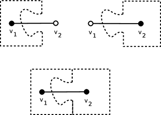
Figure 0.4: Joining two connectors to form a link

The jigsaw puzzle-piece illustration is not uncommon in the literature; such illustrations are explicitly depicted in a variety of settings.[1, 2, 3, 4] The point being illustrated here is that the connectors need not be specific vertexes, they can be vertex types, where any connector of the appropriate type is allowed to connect. This can be formalized in an expanded definition of a seed. A provisional definition of a type is needed, first.

Definition.

A type is a set of vertexes. Notationally, $t=\left\{v_{a},v_{b},\cdots\right\}$. $\diamond$

This allows the jigsaw concept to be expressed more formally.

Definition.

A seed is a vertex and the set of connector types that connect to it. That is, it is the pair $\left(v,C_{v}\right)$ where $v$ is a vertex, and $C_{v}$ is a set of connector types containing that vertex, i.e. that set of edges having $v$ as one endpoint and a type as the other endpoint. That is, $C_{v}=\left\{\left(v,t_{a}\right),\left(v,t_{b}\right),\cdots\right\}$. A single pair $\left(v,t\right)$ can be called a connector type. $\diamond$

The capital letter $C$ is used to remind one that members of the set are connectors. The intent of specifying connector types is exactly what the jigsaw-puzzle paradigm suggests: links can be created, as long as the types match up. This is formalized by expanding the definition of a link.

Definition.

Given a section $S$, a link between seeds $s_{1}=\left(v_{1},C_{1}\right)$ and $s_{2}=\left(v_{2},C_{2}\right)$ is any edge $\left(v_{1},v_{2}\right)$ where $v_{1}$ is in one of the types in $C_{2}$ and $v_{2}$ is in one of the types in $C_{1}$. That is, there exists a pair $\left(v_{1},t_{a}\right)\in C_{1}$ such that $v_{2}\in t_{a}$ and, symmetrically, there exists a pair $\left(v_{2},t_{b}\right)\in C_{2}$ such that $v_{1}\in t_{b}$ . Two seeds are connected when there is a link between them. $\diamond$

As before, the creation of links is meant to be optional, not forced. As before, the connectors are meant to be consumable: once connected, they cannot be used again. The figure below illustrates the idea.

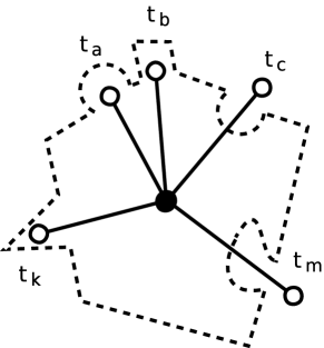
Figure 0.5: Seed connectors might be types, not vertexes

Its important to realize that the standard approach to graph theory has been left behind. Although it is possible to hook up seeds to form a graph, it is also possible to have a collection of seeds that is not a graph: the category of sections contain the category of graphs as a subset. Extending the notion of a connector to be the notion of a connector-type in particular plays considerable violence to the notion of graph theory. As long as the narrower definition of seed was used, one could imagine that a collection of seeds could be assembled into a graph, and that assembly is unique. Once connector types are introduced, the possibility that there are multiple, non-unique assemblages of seeds becomes possible. A graph can be disassembled into seeds, and, if one is careful to label vertexes and edges in a unique way, that collection can be viewed as isomorphic to the original graph. If one is not careful, sloppily assigning labels or avoiding them entirely, the collection can have multiple non-isomorphic re-assemblies. The ability to be sloppy in this way is one of the appeals, one of the benefits of working with seeds and sections. They provide “elbow room” not available in (naive) graph theory.

Why sections?

Whats the point of introducing this seemingly non-standard approach to something that looks a lot like graph theory? There are several reasons.

• From a computational viewpoint, sections have nice properties that a list of vertexes and edges do not. Given a single seed, one “instantly” knows all of the edges attached to its germ: they are listed right there. By contrast, given only a graph description, one has to search the entire list $E$ for any edges that might contain the given vertex. Computationally, searching large lists is inefficient, especially so for very large graphs.

• The subset of a section is always a section. This is not the case for a graph: given $G=\left(V,E\right)$, some arbitrary subset of $V$ and some arbitrary subset of $E$ do not generally form a graph; one has to apply consistency conditions to get a subgraph.

• A connected section behaves very much like a seed: just as two seeds can be linked together to form a connected section, so also two connected sections can be linked together to form a larger connected section. Both have a body, with spines sticking out. The building blocks (seeds), and the things built from them (sections) have the same properties, lie in the same class. Thus, one has a system that is naturally “scalable”, and allows notions of similarity and scale invariance to be explored. There is no need to introduce additional concepts and constructions.

• Given two seeds, one can always either join them (because they connect) or it is impossible to connect them. Either way, one knows immediately. Graphs, in general, cannot be joined, unless one specifies a subgraph in each that matches up. Locating subgraphs in a graph is computationally expensive; verifying subgraph isomorphism is computationally expensive.

• The analogy between graphs and topology, specifically between open sets and seeds and the intersection of open sets and edges, allows concepts and tools to be borrowed from algebraic topology.

If we stop here, not much is accomplished, other than to define a somewhat idiosyncratic view of graph theory. But that is not the case; the concept of seeds and sections are needed to pursue more complex constructions. They provide a tool to study natural language and other systems.

Example: Biochemical reaction type

An example of a seed applied to the biochemical domain would be the phosphorylation of ADP to ATP, shown in the figure below.

The germ of the seed is the point where the semi-circle kisses the line: not labeled here, the germ would be succinate-CoA ligase. The connectors are labeled with their types, and the arrows provide directionality. The connector types clearly indicate what can be linked to what: this particular seed, when linked, must link to a source of ADP, or a source of phosphate, or a sink if ATP or a sink of hydroxyls, if it is to be validly linked into any part of a connected section. In this example, ADP and ATP can both be treated as simple connectors, while R-OH does name a type: R can be any moiety. Implicit here, but not explicit in the seed, is that the R group on both connectors must be the same.

An example of a connected section would be the Krebs cycle, taken as a whole:

Each distinct reaction constitutes a seed; the heavy lines forming the cycle are the links internal to the section, and each tangent arrow is a pair of connectors, with one end of the arrow being an unconnected reaction input, and the other end of the arrow an unconnected reaction product. Thus, for example, connector types include NAD, NADH, water and ATP, among others. These connectors are free to be attached to other seeds or sections.

This example may seem dubious, at this point of the presentation. That it is a valid example should become clear with further development of the general principles in what follows.

Similar concept: Link Grammar

Readers familiar with Link Grammar[1, 5] should have recognized seeds as being more or less the same thing as “disjuncts” in Link Grammar. The formal definition for Link Grammar disjuncts are a bit more complicated than seeds, and is expanded on in later sections. To lay that groundwork, however, consider an unlabeled dependency parse for the sentence “this is an example”, shown in the figure below.

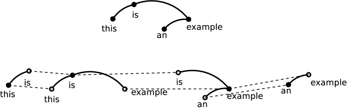
Figure 0.6: A dependency parse decomposed into four seeds

The dependency parse is shown as a graph, with four vertexes. Below, the parse is decomposed into the component seeds; as always, the open dots are connectors, the closed dots are the germs. Using the notation $\left(v,C_{v}\right)$ for a seed, where $C_{v}=\left\{\left(v,v_{a}\right),\left(v,v_{b}\right),\cdots\right\}$, these seeds can be textually written as

this: {(this, is+)}

is: {(is, this-), (is, example+)}

an: {(an, example+)}

example: {(example, is-), (example, an-)}

The above vertex: edge-list notation is a bit awkward and hard to read. A simpler notation conveying the same idea is

this: is+;

is: this- & example+;

an: example+;

example: an- & is-;

In both textual representations, the pluses and minuses are used to indicate word-order: minuses to the left, pluses to the right. This is an additional decoration added to the connectors, needed to indicate and preserve word-order, but not a part of the core definition of a seed. The ampersand is not symmetric, but enforces order; this is not apparent here, but is required for the proper definition.

In Link Grammar, the objects to the right of the colon are called “disjuncts”. The name comes from the idea that they disjoin colocational extractions. After observing a large corpus, one might find that

is: (this- & example+) or (banana- & fruit+) or (apple- & green+);

which indicates that sentences such as “a banana is a kind of fruit” or “this apple is green” were observed and parsed into (unlabeled) dependencies.

Similar concept: lambda notation

Linguistics literature sometimes describes similar concepts using a lambda-calculus notation. For example, one can sort-of envision the expression $\lambda M.xyz$ as a seed with the germ $M$ and with connectors $x$, $y$ and $z$. This notation has been used to express the concept of a seed, as described above. For example, Poon and Domingos[6] write $\lambda y\lambda x.\mbox{borders}(x,y)$ to represent the attachments of the word “borders” as a synonym for “is next to”. This is illustrated with the verb-phrase $\lambda y\lambda x.\mbox{borders}(x,y)(\mbox{Idaho})$ which beta-reduces to the verb-phrase $\lambda x.\mbox{borders}(x,\mbox{Idaho})$ to indicate that $x$ is next to Idaho. The utility of this device becomes apparent because one can use this same notation to write $\lambda y\lambda x.\mbox{is\_next\_to}(x,y)$ and $\lambda y\lambda x.\mbox{shares\_a\_border\_with}(x,y)$ as synonymous phrases. The lambda notation allows $x$ and $y$ to be exposed as connectors, while at the same time hiding the links that were required to assemble seeds for “next”, “is”, and “to” into a phrase. That is, $\lambda y\lambda x.\mbox{is\_next\_to}(x,y)$ is an example of a connected section, having $x$ and $y$ as the externally exposed connectors and the internal links between “next”, “is”, and “to” hidden.

The problem with this notation is that, properly speaking, lambda calculus is a system for generating and working with strings, not with graphs, and lambdas are designed to perform substitution (beta-reduction), and not for connecting things.

That is, lambda terms are always strings of symbols, and the variables bound by the lambda are used to perform substitutions. To illustrate the issue, suppose that $M$ above is $axbyczd$ and suppose that $\lambda N.w=ewf$. Can these be “connected” together, linked together like seeds? No: if one tried to “connect” $N$ to $z,$ one has the beta-reduction $(\lambda M.xyz)\lambda N.w\rightarrow\lambda axbycewfd.xyw$. There is no way to express some symmetric version of this, because $(\lambda N.w)\lambda M.xyz\rightarrow\lambda eaxbyczdf.xyz$ which is hardly the same. Now, of course, lambda calculus has great expressive power, and one could invent a way encoding graph theory, and/or seeds, in lambda calculus; however, doing so would result in verbose and complex system. Its easier to work with graphs directly, and just sleep peacefully with the knowledge that one could encode them with lambdas, if that is what your life depended on.

Note also that there have been extensions of the ideas of lambda calculus to graphs; however, those extensions cling to the fundamental concept of beta reduction. Thus, one works with graphs that have variables in them. Given a variable, one plugs in a graph in the place of that variable. The OpenCog http://wiki.opencog.org/w/PutLinkPutLink works in exactly this way. The beta-reduction is fundamentally not symmetrical: putting A into B is not the same as putting B into A. The concept of “connecting” in a symmetric way doesn’t arise.

Similar concept: tensor algebra

The https://en.wikipedia.org/w/Tensor_algebratensor algebra is an important mathematical construct underlying large parts of mathematical analysis, including the theory of vector spaces, the theory of Hilbert spaces, and, in physics, the theory of quantum mechanics.

Figure 0.7: A tensor with three input wires and two output wires

It has been widely noted that tensor algebras have the structure of monoidal categories; perhaps the most insightful and carefully explained such development is given by Baez and Stay[4]. The diagram of a tensor shown above is taken from that paper; it is a diagrammatic representation of a morphism $f:X_{1}\otimes X_{2}\otimes X_{3}\to Y_{1}\otimes Y_{2}$. There are several interesting operations one can do with tensors. One of them is the contraction of indexes between two tensors. For example, to multiply a matrix $M_{ik}$ by a vector $v_{k}$, one sums over the index $k$ to obtain another vector: $w_{i}=\sum_{k}M_{ik}v_{k}$. The matrix $M_{ik}$ should be understood as a 2-tensor, having two connectors, while vectors are 1-tensors. The intent here is that $M_{ik}$ is to be literally taken as a seed, with $M$ the germ, and $i$ and $k$ the connectors on the germ. The vector $v_{k}$ is another seed, with germ $v$ and connector $k$. The inner product $\sum_{k}M_{ik}v_{k}$ is a connected section. The multiplication of vectors and matrices is the act of connecting together connectors to form links: multiplication is linking.

Tensors have additional properties and operations on them, the most important of which, for analysis, is their linearity. For the purposes here, the linearity is not important, whereas the ability to contract indexes is. The contraction of indexes, that is, the joining together of connectors to form links, gives tensor algebras the structure of a monoidal category. This is a statement that seems simple, and yet carries a lot of depth. As noted above, the beta-reduction of lambda calculus also looks like the joining together of connectors. This is not accidental; rather, it is the side effect of the fact that the internal language of closed monoidal categories is simply typed lambda calculus. The words “simply typed” are meant to convey that there is only one type. For the above example morphism, that would mean that $X_{1}$ and $X_{2}$ and so on all have the same type: $X_{1}=X_{2}=X_{3}=Y_{1}=Y_{2}$. The end-points on the seed are NOT labeled; equivalently, they all carry the same label. This is in sharp contrast to the earlier example

is: this- & example+;

where the two connectors are labeled, and have different types, which sharply limit what they connect to. The this- connector has the type “this-is”, and can only attach to another connector having the same type, namely, the is+ connector on “this”

this: is+;

It may seem strange to conflate the concept of tensors and monoidal categories with linguistic analysis, yet this has an rich and old history, briefly touched on in the next section. The core principle driving this is that the Lambek calculus, underpinning the categorial grammars used in linguistic analysis, can be embedded into a fragment of non-commutative linear logic. The remaining step is to recall that linear logic is the logic of tensor categories; the non-commutative aspect is a statement that the left and right products must be handled distinctly.

Similar concept: Lambek Calculus

The foundations of categorial grammars date back to Lambek in 1961[7, 8] and the interpretation in terms of tensorial categories proliferates explosively in modern times. One direct example can be found in works by Kartsaklis[9, 3], where one can find not only a detailed development of the tensorial approach, together with its type theory, but also explicit examples, such as the tensor

$$\overrightarrow{men}\otimes\overline{built}\otimes\overrightarrow{houses}$$

together with explicit instructions on how to contract this with a different tensor

$$\mathcal{F}\left(\alpha_{\mbox{subj verb obj}}\right)=\epsilon_{W}\otimes 1_{W}\otimes\epsilon_{W}$$

to obtain the “quantization” of the sentence “men built houses”. This notation will not be explained here; the reader should consult [9] directly for details. The point to be made is that this kind of tensorial analysis can be, and is done, and often invokes words like “quantum” and “entanglement” to emphasize the connection to linear logic and to linear type theory.

Unfortunately, it is usually not clearly stated that it is only a fragment of linear logic and linear type theory that applies. In linguistics, it is not the linearity that is important, but rather the conception of frames (in the sense of Kripke frames in proof theory). Frames have the important property of presenting choices or alternatives: one can have either this, or one can have that. The property of having alternatives is described by intuitionistic logic, where the axiom of double-negation is discarded. This either-or choice appears as the concept of a “multiverse” in quantum mechanics, and far more mundanely as alternative parses in linguistics.

Another worthwhile example of tensor algebra can be found in equation 13 of [3], reproduced below:

$$\overline{verb}=\sum_{i}\left(\overrightarrow{subject}_{i}\otimes\overrightarrow{object}_{i}\right)$$

where $\overrightarrow{subject}_{i}$ and $\overrightarrow{object}_{i}$ are meant to be the $i$th occurrence of a subject/object pair in an observed corpus. If the corpus consisted of two sentences, “a banana is a kind of fruit” and “this apple is green”, then one would write

$$\overline{verb}=\left(\overrightarrow{banana}\otimes\overrightarrow{fruit}\right)+\left(\overrightarrow{apple}\otimes\overrightarrow{green}\right)$$

where the verb, in this case, is “is”. The control over the word order, that is, the left-right placement of the dependencies, is controlled by means of the pregroup grammar. The pregroup grammar and its compositionality properties follow directly from the properties of the left-division, right-division and multiplication in the Lambek calculus. A quick modern mathematical review of the axioms of the Lambek calculus can be found in Pentus[10], which also provides a proof of equivalence to context-free grammars.

Similar concept: history and Bayesian inference

Some first-principles applications of Bayesian models to natural language explicitly make use of a sequential order, called the “history” of a document.[11] That is, the probability of observing the the $n$-th word of a sequence is taken to be $P(w_{n}|h)$ where $h=w_{n-1},w_{n-2},\cdots,w_{1}$ is termed the history. This conception of probability is sharply influenced by the theory of Markov processes and finite-state machines, dating back to the dawn of information theory.[12] In a finite-state process model, the future state is predicated only on the current state, and thus the Markov assumption holds. In deciphering such a process, one might not know how the current state is correlated to the output symbol, thus leading to the concept of a Hidden Markov Model (HMM). The concept of “history” is well-suited for such analysis. Several issues, however, make this approach impractical for many common problems, including natural language.

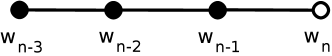
Figure 0.8: The history of a text as a sequence of words

One issue, already noted, is the sequential nature of the process. One can try to hand-wave away this issue: given a graph of vertices, it is sufficient to write the vertexes in some order, any order will do. This obscures the fact that $n$ vertexes have $n!$ ($n$-factorial) possible interactions: a combinatorial explosion, when the actual data graph may have a much much smaller number of interactions between vertexes (aka “edges”). By encoding the known interactions as edges, a graphical approach avoids such a combinatorial explosion from the outset.

To put it more bluntly: a sequential history model of genomic and proteomic data is inappropriate. Although base pairs and amino acids come in sequences, the interactions between different genes and proteins are not in any way shape or form sequential. The interactions are happening in parallel, in distinct, different physical locations in a cell. These interactions can be depicted as a graph. Curiously, that graph can resemble the one depicted below, although the depiction is meant to show something different: it is meant to show a history.

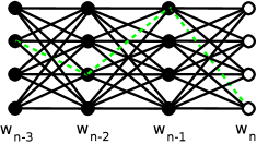
Figure 0.9: A Viterbi parse lattice of a Markov chain

Figure 0.9 depicts the lattice of a Viterbi parse of a Markov chain. The dashed green line depicts a maximum-likelihood path through the lattice, that is, the most likely history. Viterbi decoding, using an “error correcting code”, is a process by which the validity of the dashed green path is checked, and failing paths discarded. For natural language, the dashed red path must be a grammatically correct sequence of words. For a radio receiver, the dashed red path must be a sequence of bits that obey some error-correction polynomial; if it doesn’t, the next-most-likely path is selected.

Each black line represents a probability $p_{ij}$ of moving from state $i$ to state $j$ at the next time-step. That is, $p_{ij}=P(w_{n}=j|w_{n-1}=i)$ is the likelihood of word $j$ given word $i$ in the immediate past. The probabilities are arranged such that $\sum_{i}p_{ij}=1$. This is called a Markov model, because only the most recent state transitions are depicted: there are no edges connecting the nodes more than one time-step apart; there are no edges connecting $w_{n}$ to $w_{n-2},$ etc. Put differently, $P(w_{n}|h)=P(w_{n}|w_{n-1})$. That is, this depicts the use of 2-grams to predict the current state.

Non-Markov models would have edges connecting nodes further in the past. A $n$-gram approach to language digs $n$ steps into the past. If there are $k$ states, and $n$ steps into the past, then $k^{n}$ edges are required: that is, a rank-$n$ tensor. Here, $k=4$ and $n=2$ is depicted; in natural language $k$ is the number of words (say, $k=10^{4}$ for a common subset of the English language), while $n$ is the length of a longer sentence, say $n=12$. In this case, the history tensor $P(w_{n}|h)$ has $k^{n}=10^{48}=2^{160}$ edges. But of course, this is computationally absurd. It is also theoretically absurd: almost all of those edges have zero probability. Almost none of the edges are needed; the actual tensor is very very sparse.

The red path in the figure below indicates a very unlikely word-sequence: “example this an this”. There are $4\times 16=64$ paths through it. Of these, only 3 are plausible: the green edges, and the sequences “this example is an” and “an example is this”. The others can’t be observed.

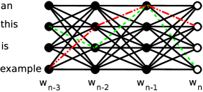
Figure 0.10: Likely and unlikely word sequences

The sparsity is easily exposed with dependency parsing. So, for example, if $w_{n-3}=this$ and $w_{n-2}=is$ and $w_{n-1}=an$, a dependency parse will tell you that $w_{n}$ must be a singular noun starting with a vowel, or an adjective starting with a vowel. It also tells you that, for this particular history, this noun can depend only on $w_{n-2}$ and on $w_{n-1}$ but not on $w_{n-3}$. A collection of dependency parses obtained from a corpus identifies which edges matter, and which edges do not.

Dependency parses do even more: they unveil possible paths, and not just pair-wise edges. They provide a more holistic view of what might be going on in natural language. That is, the notation

$$\overline{is}=\left(\overrightarrow{banana}\otimes\overrightarrow{fruit}\right)+\left(\overrightarrow{apple}\otimes\overrightarrow{green}\right)$$

and

is: (banana- & fruit+) or (apple- & green+);

and

$$P\left(w_{n}=fruit|w_{n-1}=is,w_{n-2}=banana\right)+P\left(w_{n}=green|w_{n-1}=is,w_{n-2}=apple\right)$$

all represent the same knowledge, the dependency notation appears to be less awkward than thinking about history as some Bayesian probability. The dependency notation focuses attention on a different part of the problem.

Another popular way to at least partly deal with the sparsity of the history tensor $P(w_{n}|h)$ is to use skip-grams. The idea recognizes that many of the edges of an $n$-gram will be zero, and so these edges can be skipped. This is not a bad approach, except that it is “simply typed”: it does not leverage the possibility that different words might have different types (verb, noun, …) and that this typing information delivers further constraints on the structure of the skip-gram. That is, the notion of subj-verb-obj not only tells you that your skip-gram is effectively a 3-gram, but also that the first and third words belong to a class called “noun”, and the middle is a transitive verb. This sharply prunes the number of possibilities before the learning algorithm is launched, instead of during or after. The fact that such pruning is even possible is obscured by the notation and language of $n$-grams and the history $P(w_{n}|h)$.

A different stumbling block of the “history” approach is that it ignores “the future”: the fact that the words that might be said next have already influenced the choice of the words already spoken. This can be hand-waved away by stating that the history is creating a model of (hidden) mental states, and that this model already incorporates those, and thus is anticipating future speech actions. Although this might be philosophically acceptable to some degree, it again forces complexity onto the problem, when the complexity is not needed. If you’ve already got the document, look at all of it; go all the way to the end of the sentence. Don’t arbitrarily divide it into past and future, and discard the future.

To summarize: dependency structures appear naturally; flattening them into sequences places one at a notional, computational and conceptual disadvantage, even if the flattening is conceptually isomorphic to the original problem. The tensor $P(w_{n}|h)$ may indeed encode all possible knowledge about the text in a rigorously Bayesian fashion; but its unwieldy.

Quotienting

The intended interpretation for the graphs discussed in this document is that they represent or are the result of capturing a large amount of collected raw data. From this data, one wants to extract commonalities and recurring patterns.

The core assumption being made in this section is that, when two local neighborhoods of a graph are similar or identical, then this reflects some important similarity in the raw data. That is, similarity of subgraphs is the be-all and end-all of extracting knowledge from the larger graph, and that the primary goal is to search for, mine, such similar subgraphs.

Exactly what it means to be “similar” is not defined here; this is up to the user. Similarity could mean subgraph isomorphism, or subgraph homomorphism, or something else: some sort of “close-enough” similarity property involving the shape of the graph, the connections made, the colors, directions, labels and weights on the vertexes or edges. The precise details do not matter. However, it is assumed that the user can provide some algorithm for finding such similarities, and that the similarities can be understood as a kind-of “equivalence relation”.

Example of similarity

To motivate this, consider the following scenario. One has a large graph, some dense mesh, and one decides, via some external decision process, that two vertexes are similar. One particularly good reason to think that they are similar is that they share a lot of nearest neighbors. In a social graph, one might say they have a lot of friends in common. In genomic or proteomic data, they may interact with the same kinds of genes/proteins. In natural language, they might be words that are synonyms, and thus get used the same way across many different sentences; specifically, the syntactic dependency parse links these words to the same set of heads and dependents. At any rate, one has a large graph, and some sort of equivalence operation that can decide if two vertexes are the “same”, or are “similar enough”. Whenever one has an equivalence relation, one can apply it to obtain a quotient, of grouping together into an identity all things that are the same.

To make this even more concrete, consider this example from linguistics. Suppose, given a corpus, one has observed three sentences: “Mary walked home”, “Mary ran home” and “Mary drove home”. A dependency parse provides three seeds:

walked: Mary- & home+;

ran: Mary- & home+;

drove: Mary- & home+;

which seem to be begging for an equivalence relation that will reduce these to

walked ran drove: Mary- & home+;

Using a tensorial notation, once starts with

$$\overrightarrow{Mary}\otimes\overline{walked}\otimes\overrightarrow{home}+\overrightarrow{Mary}\otimes\overline{ran}\otimes\overrightarrow{home}+\overrightarrow{Mary}\otimes\overline{drove}\otimes\overrightarrow{home}$$

and applies the equivalence relation to obtain

$$\overrightarrow{Mary}\otimes\left(\overline{walked}+\overline{ran}+\overline{drove}\right)\otimes\overrightarrow{home}$$

The structure here strongly resembles the application of the distributive law of multiplication over addition. This distributivity property is one of the appeals of the tensor notation. One can obtain a similar sense of distributivity by using the operator “or” to separate the Link Grammar style stanzas, and note that the change also appears to be an application of the distributive law of conjunction over disjunction.

This is illustrated pictorially, in figure 0.11.

Figure 0.11: Creating a quotient graph

It need not be the case that an equivalence relation is staring us in the face, yet here, it is. The vertexes “walked”, “ran” and “drove” can be considered similar, precisely because they have the same neighbors. The upper graph can be simplified by computing a quotient, shown in the lower part: the quotient merges these three similar vertexes into one. The result is not only a simpler graph, but also some vague sense that “walked”, “ran” and “drove” are synonymous in some way.

Quotienting

If one has an equivalence relation that can be applied to a graph, then the obvious urge is to attempt to perform quotienting on the graph. That is, to create a new graph, where the “equal” parts are merged into one.

The first issue to be cleared out of the way is the use of the word “https://en.wikipedia.org/wiki/Quotientquotienting”, which seems awkward, since the example above seemed to involve some sort of factoring, or the application of a distributive law of some sort. The terminology comes from modulo arithmetic, and is in wide use in all branches of mathematics. A simple example is the idea of dividing by three: given the set of integers $\mathbb{Z}$, one partitions it into three sets: the set $\left\{0,3,6,9,\cdots\right\}$, the set $\left\{1,4,7,\cdots\right\}$ and the set $\left\{2,5,8,\cdots\right\}$. These three sets are termed the cosets of 0, 1 and 2, and all elements in each set are considered to be equal, in the sense that, for any $m$ and $n$ in any one of these sets, it is always true that $m=n\mod 3$: they are equal, modulo 3. In this way, one obtains the quotient set $\mathbb{Z}_{3}=\mathbb{Z}/3\mathbb{Z}=\mathbb{Z}/\mod 3=\left\{0,1,2\right\}$. Modulo arithmetic resembles division, ergo the term “quotient”.

Given a set $S$ and an equivalence relation $\sim$, it is common to write the quotient set as $Q=S/\sim$. In the above, $S$ was $\mathbb{Z}$ and $\sim$ was $\mod 3$. In general, one looks for, and works with equivalence relations that preserve desirable algebraic properties of the set, while removing undesirable or pointless distinctions. In the modulo arithmetic example, addition is preserved: it is well defined, and works as expected. In the linguistic example, the subj-verb-obj structure of the sentence is preserved; the quotienting removes the “pointless” distinction between different verbs.

Quotienting is often described in terms of homomorphisms, functions $\pi:S\to Q$ that preserve the algebraic operations on $S$. For example, if $m:S\times S\times S\to S$ is a three-argument endomorphism on $S$, one expects that $\pi$ preserves it: that $\pi\left(m\left(a,b,c\right)\right)=m\left(\pi\left(a\right),\pi\left(b\right),\pi\left(c\right)\right)$. For the previous example, if $m$ was used to provide or identify a subj-verb-obj relationship, then, after quotienting, one expects that $m$ can still identify the verb-slot correctly.

Graph quotients

In graph theory, the notion of quotienting is often referred to as working “relative to a subgraph”. Given a graph $G$ and a subgraph $A\subset G$, one “draws a dotted line” or places a balloon around the vertexes and edges in $A$, but preserves all of the edges coming out of $A$ and going into $G$. The internal structure of $A$ is then ignored. The equivalence relation makes all elements of $A$ equivalent, so that $A$ behaves as if it were a single vertex, with assorted edges attached to it, running from $A$ to the rest of $G$.

Stalks

Given the above notion of a graph quotient, it can be brought over to the language of seeds and sections, established earlier. Let $G$ be a graph, and let $v_{a}$ and $v_{b}$ be two vertexes in the graph, with corresponding seeds $s_{a}$ and $s_{b}$ extracted from the graph. That is, $s=\left(v,C_{v}\right)$ with $C_{v}$ being the set of edges connecting $v$ to all of its nearest neighbors. Let $\pi$ be a projection function, such that $\pi\left(v_{a}\right)=\pi\left(v_{b}\right)$. That is, $\pi:V\to B$ is a map from the vertices $V$ of $G$ to some other set $B$.

It is not hard to see that $\pi$ is a morphism of graphs; it not only maps vertexes, but it can be extended to map edges as well. The target of $\pi$ is a graph quotient.

Definition.

Given a map $\pi:V\to B$, the stalk above $b\in B$ is the set $S$ of seeds such that for each $s=\left(v,C_{v}\right)\in S$, one has that $\pi(v)=b$. $\diamond$

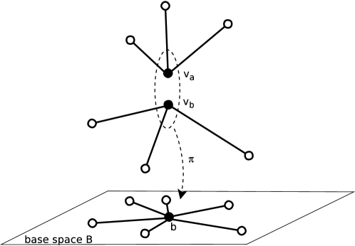
Figure 0.12: A stalk and it’s projection

In general, this definition does not require that the map $\pi:V\to B$ be a total map; that is, it does not need to be defined on all of $V$. Also, $V$ does not need to be the vertexes of some specific graph; it is enough that $V$ is a set of germs of seeds. That is, the seeds in the stalk can be generalized seeds, having typed connectors, rather than connectors derived from edges. The vertexes in the stalk can be visualized as being stacked one on top another, forming a tower or a fiber, with the edges sticking out as spines. When the seeds carry typed connectors, the stalk can be visualized as a tower of jigsaw-puzzle pieces.

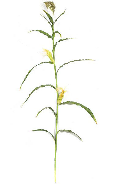
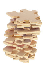
Figure 0.13: A corn stalk, a stack of puzzle pieces

Note that the projection of a stalk is a seed. It’s germ is $b$, and if any connector appears in the stalk, then it also appears as a connector on $b$ in the base. At least, this is the unassailable conclusion if one starts with a graph, and assumes that $\pi$ is a graph morphism. It will prove to be very useful to loosen this restriction, that is, to allow $\pi$ to add or remove connectors. Thus, it is useful to immediately broaden the definition of the stalk.

Definition.

Given a map $\pi:E\to B$, where both $E$ and $B$ are collections seeds, the stalk above $b\in B$ is the set $S$ of seeds in $E$ such that for each $s=\left(v,C_{v}\right)\in S$, one has that $\pi(s)=b$. $\diamond$

In this revised definition, there is no hint of what $\pi$ did with the connectors. In particular, there is no way to ask about some specific connector on some seed $s$, and what happened to it after $\pi$ mapped $s$ to $b$. This definition is perhaps too general; in the most common case, it is useful to project the connectors as well as the germs. It is also very useful to be able to say that a particular connector on $s$ can be mapped to a particular connector on $b$. Yet it is also useful to sometimes discard some connectors because they are infrequently used, to perform pruning, as it were. These use-cases will be returned to later. There is no particular reason to allow pruning during projection; it can always be done before, or after.

Thus, perhaps the most agreeable definition for a stalk is this.

Definition.

Given a map $\pi:E\to B$, where both $E$ and $B$ are collections seeds, the stalk above $b\in B$ is the set $S$ of seeds in $E$ such that for each $s=\left(v,C_{v}\right)\in S$, one has that $\pi(s)=b$. The map $\pi$ can be decomposed into a pair $\pi=\left(\pi_{g},\pi_{c}\right)$ such that, for every $\gamma\in C_{v}$ one has that $\pi\left(v,\gamma\right)=\left(\pi_{g}\left(v\right),\pi_{c}\left(\gamma\right)\right)$ such that $\pi_{c}\left(\gamma\right)\in C_{b}$. That is, $\pi_{g}$ maps the germs of $E$ to the germs of $B$ and $\pi_{c}$ maps the connectors in $E$ to specific connectors in $B$. $\diamond$

The next figure illustrates both the projection of germs, and of connectors. It tries to capture the notion that the projection is entire and consistently defined.

Figure 0.14: Germs and connectors project consistently

The definition of a link needs to be generalized, and made consistent with this final definition of a stalk.

Definition.

Two stalks $S_{1}$ and $S_{2}$ are connected if there exists a link between some seed $s_{1}\in S_{1}$ and some seed $s_{2}\in S_{2}$. The stalks are consistently linked if the projections of the stalks are also linked in a fashion consistent with the projection. That is, if $\left(v_{1},t_{a}\right)$ is the connector on $s_{1}$ that is connected to the connector $\left(v_{2},t_{b}\right)$ on $s_{2}$, viz. $v_{2}\in t_{a}$ and $v_{1}\in t_{b}$, then $\left(\pi_{g}\left(v_{1}\right),\pi_{c}\left(t_{a}\right)\right)$ is connected to $\left(\pi_{g}\left(v_{1}\right),\pi_{c}\left(t_{a}\right)\right)$ . That is, $\pi_{g}\left(v_{2}\right)\in\pi_{c}\left(t_{a}\right)$ and $\pi_{g}\left(v_{1}\right)\in\pi_{c}\left(t_{b}\right)$ .$\diamond$

Recall that the original definition of a connector was such that it could be used once and only once. This can become an issue, if it is strictly enforced on the base space. It will become convenient to remove this restriction on the base space, and replace it by a use-count. That is, if two different links between stalks project down to the same link in the base space, then the link in the base-space should be counted “with multiplicity”. This induces the notion that maybe the base space can be used for statistics-gathering, and that is exactly the intent.

Sheaves

The stalk is meant to provide a framework with which to solve the computational intractability problems associated with Bayesian networks, by explicitly exposing the grammatical structure within them in such a fashion that they can be explicitly manipulated. The intent is to accomplish the hope expressed in the diagram below. To actually arrive at a workable solution requires additional clarifications, examples, and definitions. This hopeful figure must not be taken literally: one certainly does not want the base space to be some Markov network! That would be a disaster. Rather, the hope is to accumulate a large number of graph fragments in such a way that the fragments are apparent, but that the statistics of their collective behavior is also accessible. The hope is that this can be done without overflowing available CPU and RAM, while carefully maintaining fidelity to the graph fragments. This is an example from linguistics, but one might hope to do the same with activation pathways in cell biochemistry. The citric acid cycle should be amenable to such a treatment, as well.

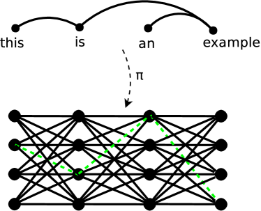
Figure 0.15: The problem, and it’s intended solution

From the previous development, it should be clear that stalks capture the local structure of graphs, and that the projection, carefully done, can preserve the essence of that local structure. Enough mechanism has been developed to allow the definition of a section to be understood in a way that is in keeping with the usual notion of a section as commonly defined in covering spaces and fiber bundles. A preliminary, provisional definition of a sheaf can now be given.

Definition.

A sheaf is a collection of connected sections, together with a projection function $\pi$ that can be taken to be an equivalence relation. That is, $\pi$ maps sections to a base space $B$, such that, for each pair of vertexes $v,w$ occurring in different sections, one has $\pi(v)=\pi(w)$ if and only if $v,w$ are in germs in the same stalk. $\diamond$

This provisional definition can be tightened. The formal definition of a sheaf also requires that it obey a set of axioms, called the gluing axioms. Before giving these, it is useful to look at an example.

Example: collocations

A canonical first step in corpus linguistics is to align text around a shared word or phrase:

	fly like a butterfly
airplanes that	fly
	fly fishing
	fly away home
	fly ash in concrete
when sparks	fly
let’s	fly a kite
learn to	fly helicopters

Each word is meant to be a vertex; edges are assumed to connect the vertexes together in some way. In standard corpus linguistics, the edges are always taken to join together neighboring words, in sequential fashion. Note that each phrase in the collocation obeys the formal definition of a section, given above. It does so trivially: its just a linear sequence of vertexes connected with edges. If the collocated phrases are chopped up so that they form a word-sequence that is exactly $n$ words long, then one calls that sequence an $n$-gram.

The projection function $\pi$ is now also equally plain: it simply maps all of the distinct occurrences of the word “fly” down to a single, generic word “fly”. The stalk is just the vertical arrangement of the word “fly”, one above another. Each phrase or section can be visualized as a botanical branch or botanical leaf branching off the central stalk.The projection of all of the stalks obtained from collocation is shown below, in figure 0.16. Identical words are projected down to a common base point. Links between words are projected down to links in the base space. For ordinary $n$-grams, the links are merely the direct sequential linking of neighboring words. The figure depicts the base-space of the sheaf obtained from $n$-grams.

Figure 0.16: N-gram corpus text alignment

The sections do not have to be linear sequences; the phrases can be parsed with a dependency parser of one style or another, in which case the words are joined with edges that denote dependencies. The edges might be directed, and they might be labeled. Parsing with a head-phrase parser introduces additional vertexes, typically called NP, VP, S and so on. The next figure (figure 0.17) shows the projection that results from alignment on an (unlabeled, undirected) dependency parse of the text. As before, each stalk is projected down to a single word, and the links are projected down as well. The most noticeable difference between this base space and the N-gram base space is that the determiner “a” does not link to “fly” even though it stands next to it; instead, the determiner links to the noun it determines. This figure also shows “ash” as modifying “fly”, which, as a dependency, is not exactly correct but does serve to illustrate how the N-gram and the dependency alignments differ. If the dependency parse produced directed edges with labels, it would be prudent to project those labels as well.

Figure 0.17: Dependency parse corpus text alignment

Both of the figures 0.16 and 0.17 depict a quotient graph that results from a corpus alignment, where all uses of a word have been collapsed (projected down) to a single node, and all links connecting the words are likewise projected. The resulting graph can be understood to depict all possible connections in a natural language. In some sense, it captures important structural information in natural language.

Be careful, though: these base spaces are just the projections of the sheaf; they are not the sheaf itself. Its as if a flashlight were held above the stalks: the base space is the shadow that is cast. The sheaf is the full structure, the base space is just the shadow.

Are projections useful?

Yes. A collapsed graph like those above might appear strange; why would one want to do that, if one has individual sentence data?

By collapsing in this way, one obtains a natural place to store https://en.wikipedia.org/wiki/Marginal_distributionmarginal distributions. For example, when accumulating statistics for large collections of sentences, the projected vertex becomes an ideal place to store the frequency count of that word; the projected edge becomes an excellent place to store the joint probability or the mutual information for a pair of words. The projected graph - the quotient graph, is manageable in size. For example, in a corpus consisting of ten million sentences, one might see 130K distinct, unique words (130K vertexes) and perhaps 5 million distinct word-pairs (5M edges). Such a graph is manageable, and can fit into the RAM of a contemporary computer.

By contrast, storing the individual parses for 10 million sentences is more challenging. Assuming 15 words per sentence, this requires storing 150M vertexes, and approximately 20 links per sentence for 200M edges. This graph is two orders of magnitude larger than the quotient graph. One could, of course, apply various programming and coding tricks to squeeze and compress the data, but this misses the point: It makes sense to project sections down to the base space as soon as possible. The original sections can be envisioned to still be there, virtually, in principle, but the actual storage can be avoided.

Every graph can be represented as an adjacency matrix. In this example, it would be a sparse matrix, with 5 million non-zero entries out of 130K$\times$130K total. The sparsity is considerable: $\log_{2}\left(130\times 130/5\right)=11.7$. Less than one in a thousand of all possible edges are actually observed.

The marginals stored with the graph can be accessed as marginals on the adjacency matrix. That is, they are marginals in the ordinary sense of values written in the margin of the matrix. Standard linear-algebra and data-analysis tools, such as the R programming language, can access the matrix and the marginals.

Visualizing Sheaves

One way of visualizing the sheaf is as a stack of sheets of paper, with one sentence written on each sheet. The papers are stacked in such a way that words that are the same are always arranged vertically one above another. This stacking is where the term “sheaf” comes from. Each single sheet of paper is a section. Each collocation is a stalk.

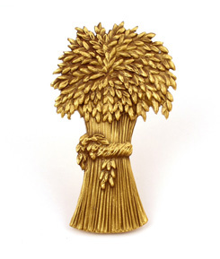
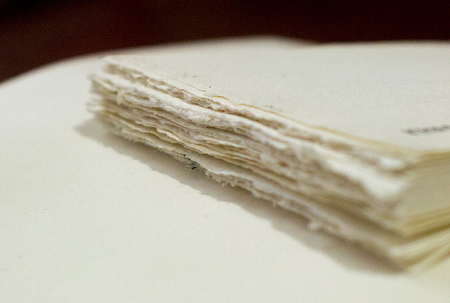
Figure 0.18: A Sheaf of Stalks; a Sheaf of Paper

A different example can be taken from biochemistry. There, one might want to write down specific pathways or interaction networks on the individual sheets of paper, treating them as sections. If one specific gene is up-regulated, one can then try to view everything else that changed as belonging to the same section, as if it were an activation mode within the global network graph of all possible interactions. Thus, for example, the Krebs cycle can be taken to be a single section through the network: it shows exactly which coenzymes are active in aerobic metabolism. The same substrates, products and enzymes may also participate in other pathways; those other pathways should be considered as other sections through the sheaf. Each substrate, enzyme or product is itself a stalk. Each reaction type is a seed.

The sheaf, it’s decomposition into sections, and it’s projection down to a single unified base network, provides a holistic view of a network of interactions. For linguistic data, activations or modes of the network correspond to grammatically valid sentences. For biological data, an activated biological pathway is a section. The base space provides a general map of biochemical interactions; it does not capture individual activations. The individual sections in the sheaf do capture that activation.

Feature Vectors

It is important to understand that, in many ways, stalks can be treated as vectors, and, specifically as the “feature vectors” of data-mining. This is best illustrated with an example.

Consider the corpus “the dog chased the cat”, “the cat chased the mouse”, “the dog chased the squirrel”, “the dog killed the chicken”, “the cat killed the mouse”, “the cat chased the cockroach”. There are multiple stalks, here, but the ones of interest are the one for the dog:

the	dog chased the cat
the	dog chased the squirrel
the	dog killed the chicken

and the stalk for the cat:

the dog chased the	cat
the	cat chased the mouse
the	cat killed the mouse
the	cat chased the cockroach

One old approach to data mining is to trim these down to 3-grams, and then compare them as feature vectors. These 3-gram feature vector for the dog is:

the	dog chased	; 2 observations
the	dog killed	; 1 observation

and the 3-gram stalk for the cat is:

chased the	cat	; 1 observation
the	cat chased	; 2 observations
the	cat killed	; 1 observation

These are now explicitly vectors, as the addition of the observation count makes them so. The vertical alignment reminds us that they are also still stalks, and that the vector comes from collocations.

Recall how a vector is defined. One writes a vector $\vec{v}$ as a sum over basis elements $\hat{e}_{i}$ with (usually real-number) coefficients $a_{i}$:

$$\vec{v}=\sum_{i}a_{i}\hat{e}_{i}$$

The basis elements $\hat{e}_{i}$ are unit-length vectors. Another common notation is the bra-ket notation, which says the same thing, but in a different way:

$$\vec{v}=\sum_{i}a_{i}\left|i\right\rangle$$

The bra-ket notation is slightly easier to use for this example. The above 3-gram collocations can be written as vectors. The one for dog would be

$$\overrightarrow{dog}=2\left|the\;*\;chased\right\rangle+\left|the\;*\;killed\right\rangle$$

while the one for cat would be

$$\overrightarrow{cat}=\left|chased\;the\;*\right\rangle+2\left|the\;*\;chased\right\rangle+\left|the\;*\;killed\right\rangle$$

The $*$ here is the wild-card; it indicates where “dog” and “cat” should go, but it also indicates how the basis vectors should be treated: the wild-card helps establish that dogs and cats are similar. It allows the basis vectors to be explicitly compared to one-another. The ability to compare these allows the dot product to be taken.

Recall the definition of a dot-product (the inner product). For $\vec{v}$ as above, and $\vec{w}=\sum_{i}b_{i}\hat{e}_{i}$, one has that

$$\vec{v}\cdot\vec{w}=\sum_{i}\sum_{j}a_{i}b_{j}\hat{e}_{i}\cdot\hat{e_{j}}=\sum_{i}\sum_{j}a_{i}b_{j}\delta_{ij}=\sum_{i}a_{i}b_{i}$$

where the Kronecker delta was used in the middle term:

$$\hat{e}_{i}\cdot\hat{e_{j}}=\delta_{ij}=\begin{cases}1&\mbox{if }i=j\\ 0&\mbox{if }i\neq j\end{cases}$$

Thus, the inner product of $\overrightarrow{cat}$ and $\overrightarrow{dog}$ can be computed:

$$\overrightarrow{cat}\cdot\overrightarrow{dog}=0\cdot 1+2\cdot 2+1\cdot 1=5$$

One common way to express the similarity of $\overrightarrow{cat}$ and $\overrightarrow{dog}$ is to compute the cosine similarity. The angle $\theta$ between two vectors is given by

$$\cos\theta=\vec{v}\cdot\vec{w}/\left|\vec{v}\right|\left|\vec{w}\right|$$

where $\left|\vec{v}\right|=\sqrt{\sum_{i}a_{i}^{2}}$ is the length of $\vec{v}$. Since $\left|\overrightarrow{cat}\right|=\sqrt{6}$ and $\left|\overrightarrow{dog}\right|=\sqrt{5}$ one finds that

$$\cos\theta=\frac{5}{\sqrt{30}}\approx 0.913$$

That is, dogs and cats really are similar.

If one was working with a dependency parse, as opposed to 3-grams, and if one used the Frobenius algebra notation such as that used by Kartsaklis in [3], then one would write the basis elements as a peculiar kind of tensor, and one might arrive at an expression roughly of the form

$$\overline{dog}=2\left(\overleftarrow{the}\otimes\overrightarrow{chased}\right)+1\left(\overleftarrow{the}\otimes\overrightarrow{killed}\right)$$

and

$$\overline{cat}=\left(\overleftarrow{chased}\otimes\overleftarrow{the}\right)+2\left(\overleftarrow{the}\otimes\overrightarrow{chased}\right)+1\left(\overleftarrow{the}\otimes\overrightarrow{killed}\right)$$

Ignoring the differences in notation (ignoring that the quantities in parenthesis are tensors), one clearly can see that these are still feature vectors. Focusing on the vector aspect only, these represent the same information as the 3-gram feature vectors. They’re the same thing. The dot products are the same, the vectors are the same. The difference between them is that the bra-ket notation was used for the 3-grams, while the tensor notation was used for the dependency parse. The feature vectors can also be written using the link-grammar-inspired notation:

dog: [the- & chased+]2 or [the- & killed+]1;

cat: [chased- & the-]1 or [the- & chased+]2 or [the- & killed+]1;

The notation is different, but the meaning is the same. The above gives two feature vectors, one for dog, and one for cat. They happen to look identical to the 3-gram feature vectors because this example was carefully arranged to allow this. In general, dependency parses and 3-grams are going to be quite different; for these short phrases, they happen to superficially look the same. In any of these cases, and in any of these notations, the concept of feature vectors remain the same.

Stalk fields and vector fields

The figures 0.16 and 0.17 illustrate the base space. Above each point in the base space, one can, if one wishes, plant a stalk.

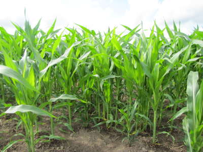
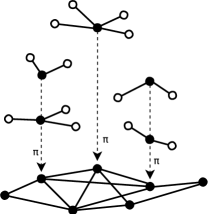
Figure 0.19: Corn field; stalk field

Such a plantation is not a sheaf; or rather it could be, but it is not one with large sections. The stalk field only has individuals seeds up and down each stalk; the stalks are not linked to one-another. In the general case, illustrated in figure 0.20, the stalks are linked to one-another; the sections really do start to resemble sheets of paper stacked one on top another.

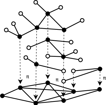
Figure 0.20: Sheafs have big sections, in general

The general sheaf, as depicted here, holds much more data than just the base space. It holds the data showing where the base space came from: how the base space was a projection of sections. Holding such a large amount of data might be impractical: in the previous example, holding the parse data for 10 million individual, distinct sentences might be a challenge. The stalk field is meant to be a half-way point: it can hold more information than the base alone, but still be computationally manageable. For example, the sme dataset discussed previously, containing 10 million sentences composed of 130K words has been found to contain 6 million seeds; these are observed on average of 2.5 times each, although the distribution is roughly Zipfian: a few are observed hundreds of thousands of times, and more than a third are observed only once.

A particular appeal of the stalk field is that each stalk can be re-interpreted as a vector. For each point of the base space, one just attaches a single vector. There is no additional structure, and all this talk of stalks can be brushed away as just a layer of theoretical complexity: in the end, its just per-base-point feature vectors.

The power of the stalk representation is to keep in mind that the basis elements are not just vacuous items, but are in fact jigsaw-puzzle pieces that can be connected to one-another. Again, each stalk can be viewed as a stack of jigsaw-puzzle pieces.

If there is a vector at each point, can the sheaf, as described here, be thought of as a fiber bundle? Maybe, but that is not the intent. In a fiber bundle, each fiber is isomorphic to every other. Thus, locally, a fiber bundle always looks like the produce space $U\times F$ with $U\subseteq B$ and $F$ the fiber. Fiber bundles are interesting when they are glued together in non-trivial ways, globally. Here, there’s a different set of concerns: its the local structure that is interesting, and not so much the global structure. Also, there has been no attempt to make each stalk (or stalk-space) isomorphic to every other. If each stalk is a vector in a vector space, one could, in principle, force that vector space to be the same, everywhere. This does not buy much: in the practical case, the support for any given vector is extremely sparse.

In some cases, it is natural to have different stalks be incomparable. In biology, some stalks may correspond to enzymes, others to RNA, others to DNA. In some vague philosophical sense, it could be argued that these are “all the same”: examples of molecules. In practice, forcing such unification seems to be a losing proposition. The goal of the technology here is to detect, observe and model fine details of structure, and not to mash everything into one bag.

Presheaves

The formal definition of a sheaf entails a presentation of the so-called “gluing axioms”. These are technical requirements that ensure that the stalks can be linked, and sections projected in a “common sense” kind of fashion. For example, if a section contains a sentence, one expects that the sentence is grammatical. One also expects to be able to extract phrases out of it. Gluing sentences together, one expects to arrive at coherent paragraphs. In a biochemical setting, one expects that all of the individual reactions in a pathway fit together. One expects to be able to talk about subsets of the full pathway without obtaining nonsense. This is just common sense.

Unfortunately, “common sense” being a commodity in short supply, the gluing axioms must be written in detail. Before this can be done, the axioms for a presheaf must be reviewed. There are several. Rather than presenting these as axioms, they are presented below as “claims”. It is up to the reader to verify that the structures defined earlier satisfy these claims. This is done for several reasons. First, such proofs are a bit tedious, and would be out of place in this otherwise rather informal treatment of the topic. Second, the overall informality of this document gives little support for weighty proofs. Third, most of these claims should be fairly self-evident, upon a bit of exploration. Finally, many choices were left to the reader: should edges be directed? Are they labeled? Do vertexes carry additional markings or values? Each choice of labeling and marking potentially affects the verification of these claims. Thus, the below are presented as “claims”, living in limbo between axioms and theorems.

First, a definition.

Definition.

An open subgraph $U$ of a graph $G$ is defined to be a section of $G$. $\diamond$

This definition helps avoid what would otherwise be confusing terminology. The open subgraphs below will always be subgraphs of the base space $B$. The open subgraphs are created by taking scissors and cutting edges in the graph, but leaving the cut half-edges attached, as they were originally. That is, the cut edges are converted into connectors. By leaving these connectors in place, much of the information needed to glue them back together remains intact. It is up to the reader to convince themselves that these open subgraphs behave essentially the same way as open sets in a topological space do: one can take intersections and unions, and doing so still results in an open subgraph. One can even build a Borel algebra out of them, but his will not be needed.

The presheaf is defined in terms of a functor and it’s properties.

Claim.

There exists a functor $F$ such that, for each open subgraph $U$ of the base graph $B$, there exists some collection $F(U)$ of sections above $U$. $\diamond$

Next, the restriction morphism, which cuts down or restricts this collection.

Claim.

For each open subgraph $V\subseteq U$ there is a morphism $\mbox{res}_{V,U}:F\left(U\right)\to F\left(V\right)$. $\diamond$

Since $V$ is smaller, we expect $F\left(V\right)$to be smaller, also. The restriction morphism trims away the unwanted parts. The trimming needs to stay faithful, to preserve the structure. Thus

Claim.

For every open subgraph $U$ of the base graph $B$, the restriction morphism $\mbox{res}_{U,U}:F\left(U\right)\to F\left(U\right)$ is the identity on $F\left(U\right)$. $\diamond$

The restrictions must compose in a natural way, as well, so that if one trims a bit, then trims a bit more, its the same as doing it all at once.

Claim.

For a sequence of open subgraphs $W\subseteq V\subseteq U$, the restrictions compose so that $\mbox{res}_{W,V}\circ\mbox{res}_{V,U}=\mbox{res}_{W,U}$. $\diamond$

If a system obeys the above, it is technically called a presheaf. A presheaf is much like the (informal) definition given for a sheaf, above. However, it is possible to create structures that satisfy the above claims (axioms), but don’t quite match the intended definition of a sheaf. In particular, the above are not enough to guarantee that the sections in the presheaf can be organized properly into stalks. To get well-behaved stalks, more is needed. These are the gluing axioms.

Gluing axioms

The open subgraphs behave much like open sets. Thus, the concept of an open covering can be imported in a straight-forward way. A collection $\left\{U_{i}\right\}$ of open subgraphs is an open cover for an open subgraph $U$ if the union of all the $U_{i}$ contain $U$. That is, they are an open cover if $U\subseteq\bigcup_{i}U_{i}$. The union of open subgraphs is meant to be “obvious”: join together the connectors, where possible.

A presheaf is a sheaf if it obeys the following two claims/axioms.

Claim.

(Locality) If $\left\{U_{i}\right\}$ is an open cover for $U$, and if $s,t\in F\left(U\right)$ are sections such that $s|_{U_{i}}=t|_{U_{i}}$ for each $U_{i}$, then $s=t$. $\diamond$

In the above, the notation $s|_{V}$ denotes the restriction of the section $s$ to the open subgraph $V$ of the base space $B$. Pictorially, $s|_{V}$ is that part of the section that sits on the stalks above $V$. It is a trimming-down of $s$ so that it projects cleanly down to $V$ and to nothing larger. If each $U_{i}$ is a seed in the base space, then $s|_{U_{i}}$ is a seed in the stalk above $U_{i}$. Note that $s|_{U_{i}}$ might be the empty set. The locality axiom is basically saying “stalks exist”. Alternately, the locality axiom says that if you cut up a layer-cake, you can still tell, after the cutting, which layer was which.

The gluing axiom is needed to reassemble the pieces.

Claim.

(Gluing) If $\left\{U_{i}\right\}$ is an open cover for $U$, and if $s_{i}\in F\left(U_{i}\right)$ are sections restricted to each $U_{i}$, and if, for all pairs $i,j$ the $s_{i}$ and $s_{j}$ agree on overlaps, then there exists a section $s\in F\left(U\right)$ such that $s_{i}=s|_{U_{i}}$. $\diamond$

In the above, the phrase “$s_{i}$ and $s_{j}$ agree on overlaps” means that $s_{i}|_{U_{i}\cap U_{j}}=s_{j}|_{U_{i}\cap U_{j}}$. Note that $U_{i}\cap U_{j}$ might be the empty set, in which case no agreement is needed. The gluing axioms states, more or less, that if the layer cake is cut into pieces, and the pieces can be reassembled with the edges lining up correctly, then the original layers can be re-discovered.

Gluing is perhaps not as trivial as it sounds. It will be seen later on that gluing is essentially the same thing as parsing. Obtaining a successful parse is the same thing as assembling a valid section ut of the parts. In the case of natural language, a parse succeeds if and only if a sentence is grammatically valid. But of course! The sections of a natural language sheaf are exactly the grammatical sentences.

Until this more detailed presentation of parsing is described, one can imagine the following scenario. If seeds correspond to jigsaw-puzzle pieces, then the sections $s_{i}$ correspond to partially-assembled parts of the jigsaw. Two such parts $s_{i}$ and $s_{j}$ agree on overlaps if $U_{i}\cap U_{j}$ is non-empty, and these two parts can be joined together. If the connectors are typed, then there may be multiple distinct connectors that can be joined to one-another. They just might fit. That is, there might be more than one way to make $s_{i}$ and $s_{j}$ connect, possibly by shifting, turning, the pieces, etc. If one then tried to connect $s_{k}$, there might be multiple ways of doing this, leading to a combinatorial explosion. At some point in this process, one might discover that there is simply no way at all to connect the next piece: it just won’t fit. One then has to back-track, and try a different arrangement. Obtaining an efficient algorithm to perform this back-tracking is non-trivial: such algorithms are called parsers, and gluing is parsing.

Does this really work?

The sheaf axioms presented above are standardized and are presented in many books. See, for example, Eisenbud & Harris[13] or Mac Lane & Moerdijk[14]. The point of the above is to convince the reader that the structures being described really are sheaves, in the formal sense of the word. There’s a big difference though: everything above was developed from the point of view of graphs, and that really does change the nature of the game. That said, the reason that all of this machinery “works” is because the open subgraphs really do behave very much like open sets. Because of this, many concepts from topology extend naturally to the current structures.

This is not exactly a new realization. The “open subgraphs” defined here essentially form a https://en.wikipedia.org/wiki/Grothendieck_topologyGrothendieck topology, and the thing that is being called a “sheaf” should probably be more accurately called a “site”. Developing and articulating this further is left for a rainy day.

It is worth noting at this point that the normal notion of a “germ” in sheaf theory corresponds to what is called a “seed”, here. I suppose that the vocabulary used here could be changed, but I do like thinking of seeds as sticky burrs. The biological germ of a seed is that thing left, when the outer casing is removed.

The use of the jigsaw-puzzle piece analogy to define connectors is strongly analogous to the construction of the https://en.wikipedia.org/wiki/Nerve_of_a_coveringČech nerve. This can be thought of as a way of inducing overlaps from fiber products. This point is returned to, later on.

Cohomology

In orthodox mathematics, the only reason that sheaves are introduced is to promptly usher the reader to Čech cohomology in the next chapter of any book on algebraic topology. That won’t be done here, so what’s the point of all this?

Well, this won’t be done here mostly because I’m running out of space, and, in the context of biology and linguistics, this is uncharted territory. But some comments are in order. First, if the point of this was merely to get at graph theory, there would not be much to say. For example, the homotopy theory of graphs is more-or-less boring: every graph is homotopic to a bouquet of circles. Homotopy and homology on graphs only becomes interesting if one can add 2-cells and $n$-cells for $n>1$; then one gets cellular homology. Can that ever happen here?

If one considers biochemistry, and use the Krebs cycle (the citric acid cycle) as an example, then the answer is yes. This is a loop; it’s essentially exothermic, or a kind of pump, in that the loop always goes around in one direction. The edges are directional. Its a cycle not only in a biological sense, but also in the mathematical sense: it can be considered to be the boundary of a 2-cell. The Krebs cycle is not the only cycle in biochemistry, and many of these cycles share common edges. In essence, there’s a whole bunch of 2-cells in biochemistry, and they’re all tangent to one-another. That is, there are chain complexes in biochemistry. Is there interesting homology? Perhaps not, as this would require some 2-cells to run “backwards”, and that seems unlikely. That would imply that there are no 3-cells in biochemistry. But who knows; we have not had the tools to “solve biochemistry” before.

What about linguistics? Examples here seem to be more forced. Yes, dependencies can be directional. Dependency trees are trees, however. One can allow loops in them, but these loops are always acyclic. (viz. a “DAG” - a directed acyclic graph). There are no obviously cyclic phenomena in natural language.

Why sheaves?

By pointing out that natural language and biology can be described with sheaves, it is hoped that this will prove better insights into their structure, and provide a clear framework to think about the structure of such data.

For example, consider the normally vague idea of the “language graph”. What is this? One has dueling notions: the graph of all sentences; the generative power of grammars. Sheaves provide a clearer picture: the graph itself is the base space, while surface and deep structure can be explored through sections.

It can be argued that orthodox corpus linguistics studies the sheaf of surface structure, with especially strong focus on the stalks. Differences in the stalks reveal differences between regional dialects. Much more interesting is that the corpus linguists have analyzed stalks to discover not just differences in socio-economic status, but even to discover politically-motivated speech, truth and lack-thereof in journalism and news media.[15]

The orthodox corpus linguists are not interested in refining their collocations into a generative grammar. One does not obtain a generative model of how different speakers in different socio-economic classes speak; corpus linguistics examples are just that: examples that are not further refined. By applying a pattern mining approach, the underlying grammar can be discovered computationally. By viewing structure holistically, as a sheaf, one can see ways in which this might be done.

Besides the sheaf of surface realizations studied by corpus linguists, there are several different kinds of sheaves of grammatical structure. Each section is a grammatically valid sentence, expressed as a tree or as a DAG (directed acyclic graph) of some sort, annotated with additional information, based on the formalities of that particular grammatical approach (dependency grammar, head-phrase-structure grammar, etc). The orthodox approach is to view the grammar as being the primary object of study. The sheaf approach helps emphasize how that grammar was arrived at: distinct words were grouped into grammatical classes. Put differently, distinct stalks are recognized as being very similar, if not identical, and are merged together to form a grammatical category; it is no longer individual words that link with one-another, but the grammatical classes.

Viewing language as a sheaf helps identify how one can automatically extract grammatical classes: If one can judge two stalks as being sufficiently similar in some way, then one can merge them into one, proceeding in this way to create a reduced, concentrated model of language that captures it’s syntactic structure.

One can do even more: one can play off the differences in regional dialects, or differences due to social-economic classes, discovered by statistical means from a corpus, and attach these to specific grammatical structures, identified from syntactic analysis. That is, by seeing both activities: surface realizations and deeper structure as two slightly different forms of “the same thing”, one can see-saw, lever ones way about, moving from one to the other and back. Tools can be developed that do both, instead of just one or just the other. One can actually unify into one, what seem to be very theories and approaches, and one can develop the techniques to move between these theories. This seems to be a very big win.

clustering morphisms

The primary topic of this part is that the extraction of structure from data is more-or-less a kind of morphism between sheaves. A “pseudo-morphism” might be an more appropriate term, as the definition here will not be axiomatically precise.

There are several types of morphisms that are of interest. one kind keeps the base space intact, but attempts to map one kind of section into another: for example, mapping sections of $n$-grams into sections of dependency parses. This resembles the orthodox concept of a morphism between sheaves. The other kind of morphism is one that attempts to re-arrange the base space, by grouping together multiple stalks into one. This second kind of morphism is the one discussed in this part. It is roughly termed a “clustering morphism”.

There are several kinds of clustering morphisms that are interesting. One was previously illustrated. Starting with

$$\overrightarrow{Mary}\otimes\overline{walked}\otimes\overrightarrow{home}+\overrightarrow{Mary}\otimes\overline{ran}\otimes\overrightarrow{home}+\overrightarrow{Mary}\otimes\overline{drove}\otimes\overrightarrow{home}$$

one wishes to deduce

$$\overrightarrow{Mary}\otimes\left(\overline{walked}+\overline{ran}+\overline{drove}\right)\otimes\overrightarrow{home}$$

This seems to be relatively straight-forward to accomplish, as it looks like a simple application of the distributive law of multiplication over addition. It is perhaps deceptive, as it presumes that the three words “walked”, “ran”, “drove” do not appear anywhere else in the sheaf.

A different example is that of forcing diagonalization where there is none. Given a structure such as

$$\left|Mary\right\rangle\otimes\left|walked\right\rangle+\left|Adam\right\rangle\otimes\left|ran\right\rangle$$

one wishes to induce

$$\left(\left|Mary\right\rangle+\left|Adam\right\rangle\right)\otimes\left(\left|walked\right\rangle+\left|ran\right\rangle\right)$$

This resembles a grammar-school error: an inappropriate application of the distributive law. But is it really? Part of the problem here is that the notation itself is biased: the symbols $\otimes$ and $+$ look like the symbols for multiplication and addition, and we are deeply ingrained, from childhood - from grammar school, that multiplication distributes over addition, but not the other way around. By using these symbols, one introduces a prejudice into one’s thinking; the prejudice suggests that one operation is manifestly legal, while the other is dubious and requires lots of justification.

This prejudice can run very deeply: in data-mining software, if not in the theories themselves, the first operation might be hard-coded into the software, into the theory, and assumed to be de facto correct. By contrast, the second relation seems to require data-mining, and maybe lots of it: crunching immense, untold numbers of examples to arrive at the conclusion that such a diagonalization is valid. Perhaps reality is somewhere between these two extremes: the first factorization should not be assumed, and, as a result, the second diagonalization might not be so hard to discover. Perhaps induction can be applied uniformly to both cases.

Induction

The goal of machine learning in data science is the induction of the factorization and diagonalization from a given dataset. Both examples given above are misleading, because they ignore the fact that they are embedded in a much larger corpus of language. How might these two cases be induced from first principles, ab initio, from nothing at all, except for a bunch of examples?

On possibility is to start by looking for pair-wise correlations. This works: that is how $\left|Mary\right\rangle\otimes\left|walked\right\rangle$ is discovered in the first place: these two words were collocated. Likewise, for $\left|Adam\right\rangle\otimes\left|ran\right\rangle$. But what about inducing diagonalization? Here, one observes that Mary does lots of things, and so does Adam. Writing down the collocation stalk for Mary, and the one for Adam should indicate that these two stalks are quite similar. How can similarity be judged? The cosine distance, previously reviewed, is a plausible way to start. One can legitimately conclude that Adam and Mary belong in the same grammatical category. What about “walked” and “ran”? One can create a stalk for these two as well, and it should not be hard to conclude, using either cosine distance, or something else, that the two are quite similar.

Great. Now what? Just because Adam and Mary are similar, and “ran” and “walked” are similar, this is still not quite enough to justify the diagonalization. After all, “Mary ran” and “Adam walked” have not been observed; how can one justify that these will likely be observed, which is the central claim that diagonalization is making?

The answer would need to be that certain cross-correlations are only weakly seen. Define the set of named-things, and action-things, already discovered: $names=\{Adam,Mary\}$ while $actions=\{ran,walked\}$. Let the $\lnot$ symbol denote “not”, so that $\lnot names$ is the set of all things are not $names$, and $\lnot actions$ denote all things that are not actions. Consider then the correlation matrix

	$actions$	$\lnot actions$
$names$	High	Low
$\lnot names$	Low	n/a

The entry “High” means that a large amount of correlation is observed, while “Low” means that little is observed. Correlation can be measured in many ways; mutual information and Kullbeck-Liebler divergence are popular.

Why might this work? The point is that if $\lnot actions$ contains words like $book$ or $tree$, then sentences like “Mary book” or “Adam tree” are not likely to be observed; if $\lnot names$ includes words like $green$ or $the$, then sentences like “green walked” or “the ran” should be rare.

The correlation matrix embodies the very meaning of “diagonalization”: a matrix is diagonal, when the entries along the diagonal are large, and the entries not on the diagonal are zero. Observing this structure then justifies writing $names\otimes actions$, which is exactly what one wanted to induce. Can one also validly claim that $\left(\lnot names\right)\otimes\left(\lnot actions\right)$? Well, probably not. The correlation there might be low - pairs would be inconsistent as to how compatible they are. It might be hard to compute, and, in the current context, it seems not to be wanted.

Can one induce factorization in the same way? Factorization, as given above, seemed “obvious”, but that was only due to the use of symbols that prejudiced one’s thinking. Factorization is, in fact, every bit as non-obvious as diagonalization. The reason it seems so obvious in the example was that the corpus “Mary walked home”, etc. did not include any sentences about Adam, nor anything about “to the store”, “to work”, etc. Once these are included, factorization starts to look a lot like diagonalization, if not exactly the same thing. Inducing a subject-verb-object relationship can be done by means of correlation, but is harder to depict, because the correlation is no longer a pair-wise matrix, but is 3D, forming a cube, because three categories need to be compared: $names$, $actions$, and $places$, where $places=\{home,to\,the\,store,to\,work\}$. This is shown below.

$places\;\begin{cases}\\ \\ \\ \end{cases}$ $actions$ $\lnot actions$ $names$ High Low $\lnot names$ Low n/a

$\lnot places\;\begin{cases}\\ \\ \\ \end{cases}$ $actions$ $\lnot actions$ $names$ Low n/a $\lnot names$ n/a n/a

That is, one can induce a three-way relationship $(x,y,z)$ whenever that relationship is frequently seen, and all three of the relations $(\lnot x,y,z)$, $(x,\lnot y,z)$ and $(x,y,\lnot z)$ are not seen. This extends to 4-way relations, and so on.

There is one notable phenomenon that is not covered by the above: words that have different meanings, but the same spelling, for example, “saw” or “fly” which are both nouns and verbs. This complicates the approach above; this issue is returned to in a later section, titled sec:Polymorphism.

Related concept: Discrimination

Several comments are in order. The above presents grammatical induction as a form of discrimination - https://en.wikipedia.org/wiki/Binary_classificationbinary discrimination, even, which is considered to be a particularly simple form of learning. There are many available techniques for this, and one can promptly fall into the examination of https://en.wikipedia.org/wiki/Receiver_operating_characteristicROC curves, and the like. It is important to note that what is being sketched here is the idea of discrimination in the context of sheaves, and not the idea of binary discrimination as some panacea for linguistics.

The above was also vague as to the form of correlation: how should it be done? Should it literally be correlation, in the sense of probability theory? Should it be mutual information? Something else? This is left intentionally vague: different measures of correlation are possible. Some may produce better results than others. A general theoretical framework is being sketched here; the quality of different algorithms is not assessed or presented. It is up to the reader to experiment with different forms of correlation and discrimination.

Related concept: Clustering

The induction, described above, resembles the machine-learning concept of clustering in several ways. There are also some strong differences, and so this is worth reviewing. Two old and time-honored approaches to clustering are support vector machines (SVM) and $k$-means clustering. The first relies explicitly on some sort of vectorial representation for the data, while the second expects some sort of metric for judging whether two points are similar or not. For the former, interpreting the stalks as the feature vectors is sufficient, while for the latter, the cosine distance can fill the role of a metric.

These two approaches are sufficient to extract classes of things, such as $names$, $places$ and $actions$ in the above example. The accuracy of the extracted categories is rarely excellent, but is certainly adequate enough to proceed to other stages. Except … that’s it. These clustering techniques stop there; they say nothing at all about inducing grammatical relations. To induce grammatical relations, one also has to perform discrimination in some way. One has to combine the results obtained from clustering, and then discriminate to induce grammar.

Note that the discrimination step provides information about how good the clustering was. Say, for example, that cosine distance was used, together with $k$-means clustering, to obtain classes of words. Was this clustering “adequate”? That question can be answered by examining the ROC curves obtained from a binary discrimination step. Different kinds of clustering will present different ROC curves. This can be used as feedback for the clustering step, so that one gets a recursive learning step, alternating between discrimination and clustering.

This observation of recursion, of course, raises the question: can clustering and discrimination be combined into one effective algorithm? Yes, they can.

Related concepts: neurlal nets, adagram.

Besides binary discrimination, there are other approaches. Approaches that are more sophisticated include decision trees and decision forests. These two approaches treat the vectors as tables of input data, and then pick and choose among the vector components deemed predictive.

x

x

foo

orig neural net: [Bengio2003]

More

This: https://becominghuman.ai/how-does-word2vecs-skip-gram-work-f92e0525def4

Why clustering?

foo-bar

x

x

By contrast, the goal here is not just to talk about a graph $G$ relative to a single $A$, but relative to a huge number of different $A$’s. What’s more, the internal structure of these $A$’s will continue to be interesting, and so is carried onwards. Finally, the act of merging together multiple vertexes into one $A$ may result in some of the existing edges being cut, or new edges being created. The clustering operation applied to the graph alters the graph structure. These considerations are what makes it convenient to abandon traditional graph theory, and to replace it by the notion of sheaves and sections.

x

The above establishes a vocabulary, a means for talking about the clustering of similar things on graphs. It does not suggest how to cluster. Without this vocabulary, it can be very confusing to visualize and talk about what is meant by clustering on a graph. Its worth reviewing some examples.

• In a social graph, a cluster might be a clique of friends. By placing these friends into one group, the stalk allows you to examine how different groups interact with one-another.

• In proteomic or genomic data, if one can group together similar proteins or genes into clusters, one can accomplish a form of dimensional reduction, simplifying the network model of the dataset. It provides a way to formalize network construction, without the bad smell of ad-hoc simplifications.

• In linguistic data, the natural clustering is that of words that behave in a similar syntactic fashion; such clusters are commonly called “grammatical classes” or “parts of speech”. In particular, it allows one to visualize language as a graph. So: consider, for example, the set of all dependency parses of all sentences in some corpus, say Wikipedia. Each dependency parse is a tree; the vertexes are words, and the edges are the dependencies. Taken as a graph, this is a huge graph, with words connecting to other words, all over the place. Its not terribly interesting in this raw state, because its overwhelmingly large. However, we might notice that all sentences containing the word “dish” resemble all sentences containing the word “plate”; that these two words always get used in a similar or the same way. Grouping these two words together into one reduces the size of the graph by one vertex. Aggressively merging similar words together can sharply shrink the size of the graph to a manageable size. One gets something more: the resulting graph can be understood as encapsulating the structure of the English language.

This last example is worth expanding on. Two things happen when the compressed graph is created. First, that graph encodes the syntactic structure of the language: the links between grammatical classes indicate how words can be arranged into grammatically correct sentences. Second, the amount of compression applied can reveal different kinds of structures. With extremely heavy compression, one might discover only the crudest parts of speech: determiners, adjectives, nouns, transitive and intransitive verbs. Each of these classes are distinct, because they link differently. However, if instead, a lot less compression is applied, then one can discover synonymous words: so, “plate” and “dish” might be grouped together, possibly with “saucer”, but not with “cup”. Here, one is extracting a semantic grouping, rather than a syntactic grouping.

So, the answer to “why clustering?” is that it allows information to be extracted from a graph, and encoded in a useful, usable fashion. No attempt is made here to suggest how to cluster; merely, that if an equivalence relation is available, and if it is employed wisely, then one can construct quotient graphs that encode important relationships of the original, raw graph.

Types

It is notationally awkward to have to write stalks in terms of the sets of vertexes that they are composed of; it is convenient to instead replace each set by a symbol. The symbol will be called a type. As it happens, these types can be seen to be the same things occurring in the study of type theory; the name is justified.

The core idea can be illustrated with Link Grammar as an example. The Link Grammar disjuncts are one and the same thing as stalks. It is worth making this very explicit. A subset of the Link Grammar English dictionary looks like this:

cat dog: D- & S+;

the a: D+;

ran: S-;

This states that “cat” and “dog” are both vertexes, and they are in the same stalk. That stalk has two connectors: D- and S+, which encode the other stalks that can be connected to. So, the D+ can be connected to the D- to form a link. The link has the form ({the, a}, {cat, dog}) and the connector symbols D+ and D- act as abbreviations for the vertex sets that the unconnected end can connect to. The + and - symbols indicate a directionality: to the right or to the left. The capture the notion that, in English, the word-order matters. To properly explain the + and -, we should have to go back to the definition of a graph on the very first page, and introduce the notion of left-right order among the vertices. Doing so from the very beginning would do nothing but clutter up the presentation, so that is not done. The reader is now invited to treat the initial definition of the graph as a monad: there are additional details “under the covers”, but they are wrapped up and ignored, and only the relevant bits are exposed. Perhaps the vertices had a color. Perhaps they had a name, or a numerical weight; this is ignored. Here, we unwrap the idea that the vertices must be organized in a left-right order. Its sufficient, for now, to leave it at that.

Figure 0.21: Three stalks and two typed links

The three stalks here encode a set of grammatically valid English language sentences. Hooking together the S- and S+ connectors to form an S link, one obtains the sequence [{the, a} {cat, dog} {ran}]. This can be used to generate grammatically valid sentences: pick one word from each set, and one gets a valid sentence. Alternatively, this structure can be taken to encode the sum-total knowledge about this toy language: it is a kind-of graphical representation of the entire language, viewed as a whole.

Definition.

Given a stalk $S=\left(V,L\right)$, the connector type of $L$ is a symbol that can be used as a synonym for the set $L$. It serves as a short-hand notation for $L$ itself. $\diamond$

Just as in type theory, a type can be viewed a set. Yet, just as in type theory, this is the wrong viewpoint: a type is better understood as expressing a property: it is an intensional, rather than an extensional description. Formally, in the case of finite sets, this may feel like splitting hairs. For an intuitive understanding, however, its useful to think of a type as a property carried by an object, not just the class that the object can be assigned to.

Why types?

Types are introduced here primarily as a convenience for working with stalks. They are labels, but they can be useful. Re-examining the examples:

• In a social graph, one group of friends might be called “students” and another group of friends might be called “teachers”. The class labels are useful for noting the function and relationship of the different social groups.

• In a genetic regulatory network, sub-networks can be classified as "positive regulatory pathways" or "negative regulatory pathways" with respect to the activation of a particular gene.

These examples suggest that the use of types is little more than a convenient labeling system. In fact, more hay can be made here, as types interact strongly with category theory: types are used to describe the internal language of monoidal categories. But this is a rather abstract viewpoint, of no immediate short-term use. Suffice it to say that appearance of types in grammatical analysis of a language is not accidental.

What kind of information do types carry?

The above example oversimplifies the notion of types, presenting them as a purely syntactic device. In practice, types also carry semantic information. The amount of semantic information varies inversely to the broadness of the type. In language, coarse-grained types (noun, verb) carry almost no semantic information. Fine-grained types carry much more: a “transitive verb taking a particle and an indirect object” is quite specific: it must be some action that can be performed on some object using some tool in some fashion. An example would be “John sang a song to Mary on his guitar”: there is a what, who and and how yoked together in the verb “sang”. The more fine-grained the classification, the more semantic content is contained in it.

This suggests that the proper approach is hierarchical: a fine-grained clustering, that captures semantic content, followed by a coarser clustering that erases much of this, leaving behind only “syntactic” content.

Parsing

The introduction remarked that not every collection of seeds can be assembled in such a way as to create a valid graph. This idea can be firmed up, and defined more carefully. Generically, a valid assembly of seeds is called a parse, and the act of assembling them is called parsing, which is done by parse algorithms. To illustrate the process, consider the following two seeds:

$v_{2}:\left\{\left(v_{2},v_{1}\right),\left(v_{2},v_{3}\right)\right\}$

$v_{3}:\left\{\left(v_{3},v_{2}\right)\right\}$

Represented graphically, these seeds are

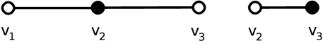
Figure 0.22: Two unconnected seeds

The connector (half-edge) $\left(v_{2},v_{3}\right)$ appears with both polarities, and can be linked together to form a link. The connector $\left(v_{2},v_{1}\right)$ has nothing to connect to. Even after maximally linking these two seeds, one does not obtain a valid graph: the vertex $v_{1}$ is missing from the vertex-set of the graph, even though there is an edge ready to attach to it. This provides an example of a failed parse. It is enough to add the seed $v_{1}:\left\{\left(v_{1},v_{2}\right)\right\}$ to convert this into a successful parse. Adding this seed, and then attempting to maximally link it results in a valid graph; the parse is successful.

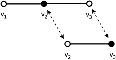
Figure 0.23: Parsing is the creation of links

Note the minor change in notation: the colon is used as a separator, with the germ appearing on the left, and set of connectors on the right. The relevance of this notational change becomes more apparent, if we label the vertexes in a funny way: let $v_{1}$ carry the label “the”, and $v_{2}$ carry the label “dog” and $v_{3}$ carry the label “ran”. The failed parse is meant to illustrate that “dog ran” is not a grammatically valid sentence, whereas “the dog ran” is.

Converting these seeds to also enforce left-right word-order requires the notation

the: {(the, dog+)}

dog: {(dog, the-), (dog,ran+)}

ran: {(ran, dog-)}

This notation is verbose, and slightly confusing. Repeating the germ as the first vertex in every connector is entirely unnecessary. Write instead:

the: { dog+ }

dog: { the-, ran+}

ran: { dog- }

The set-builder notation is unneeded, and perhaps slightly confusing. In particular, the word “dog” has two connectors on it; both must be connected to obtain a valid parse. The ampersand can be used to indicate the requirement that both connectors are required. This notation will also be useful in the next section.

the: dog+ ;

dog: the- & ran+ ;

ran: dog- ;

This brings us almost back to the previous section, but not quite. Here, we are working with seeds; previously we worked with stalks. Here, the connector type labels were not employed. In real-world use-cases, using stalks and type labels is much more convenient.

This now brings us to a first draft of a parse algorithm. Given an input set of vertices, it attempts to find a graph that is able to connect all of them.

1. Provide a dictionary $D$ consisting of a set of unconnected stalks.

2. Input a set of vertices $V=\left\{v_{1},v_{2},\cdots,v_{k}\right\}$.

3. For each vertex in $V$, locate a stalk which contains that vertex in it’s germ.

4. Attempt to connect all connectors in the selected stalks.

5. If all connectors can be connected, the parse is successful; else the parse fails.

6. Print the resulting graph. This graph can be described as a pair $\left(V,E\right)$ with $V$ the input set of vertexes, and $E$ the set of links obtained from fully connecting the selected stalks.

The above algorithm is “generic”, and does not suggest any optimal strategy for the crucial steps 3 or 4. It also omits discussion of any further constraints that might need to be applied: perhaps the edges need to be directed; perhaps the resulting graph must be a planar graph (no intersecting edges); perhaps the graph must be a minimum spanning tree; perhaps the input vertexes must be arranged in linear order. These are additional constraints that will typically be required in some specific application.

Why parsing?

The benefit of parsing for the analysis of the structure of natural language is well established. Thus, an example of parsing in a non-linguistic domain is useful. Consider having used the above graph compression/vertex-edge clustering techniques to obtain a collection of stalks that describe genomic interactions. This collection provides the initial dictionary $D$. Now imagine a process where a certain specific set of genes are associated with some particular trait or reaction. Is this a complete set? Can it be said that their interactions are fully understood?

One way to answer these last two questions would be to apply the parse algorithm, using the known dictionary, to see if a complete interaction network can be obtained. If so, then this new specific gene-set fits the general pattern. If not, if a complete parse cannot be found, then one strongly suspects that there remain one or more genes, yet undetermined, that also play a role in the trait. To find these, one might examine the stalks that might have been required to complete the parse: these will give hints as to the specific type of gene, or style of interaction to search for.

Thus, parsing new gene expressions and pathways offers a way of discovering whether they resemble existing, known pathways, or whether they are truly novel. If they seem novel, parsing also gives strong hints as to where to look for any missing pieces or interactions.

Is this really parsing?

The above description of parsing is sufficiently different from standard textbook expositions of natural language parsing that some form of an apology needs to be written.

The first step is to observe that the presented algorithm is essentially a simplified, generalized variation of the Link Grammar parsing algorithm.[5] The generalization consists in the removal of word-order and link-crossing constraints.

The second step is to observe that the theory of Link Grammar is more-or-less isomorphic to the theory of pregroup grammars[3] (see https://en.wikipedia.org/wiki/Pregroup_grammarWikipedia); the primary differences being notational. The left-right directional Link Grammar connectors correspond to the left and right adjoints in a pregroup. A Link Grammar disjunct (that is, a seed) corresponds to a sequence of types in a pregroup grammar. The correspondence is more-or-less direct, except that link grammar is notationally simpler to work with.

The third step is to observe that the Link Grammar is a form of dependency grammar. Although the original Link Grammar formulation uses undirected links, it is straight-forward and unambiguous to mark up the links with head-dependent directional arrows.

The fourth step is to realize that dependency grammars (DG) and head-phrase-structure grammars (HPSG) are essentially isomorphic. Given one, one can obtain the other in a purely mechanistic way.

The final step is to realize that most introductory textbooks describe parsers for a context-free grammar, and that, for general instructional purposes, such parsers are sufficient to work with HPSG. The priamry issue with HPSG and context-free language parsers is that they obscure the notion of linking together pieces; this is one reason why dependency grammars are often favored: they make clear that it is the linkage between various words that has a primary psychological role in the human understanding of language. It should be noted that many researchers in the psychology of linguistics are particularly drawn to the categorial grammars; these are quite similar to the pregroup grammars, and are more closely related to Link Grammar than to the phrase-structure grammars.

Polymorphism

Any given vertex may participate in two or more seeds, independently from one-another. It is this statement that further sharpens the departure from naive graph theory. This is best illustrated by a practical example.

Consider a large graph, constructed from a large corpus of English language sentences. As subgraphs, it might contain the two sentences “A big fly landed on his nose” and “It will fly home”. The vertex “fly” occurs as a noun (the subject, with dterminer and adjective) in one sentence, and a verb (with subject and object) in the other. Suppose that the equivalence relation, described in the clustering section, also has the power to discern that this one word should really be split into two, namely $fly_{\mbox{noun}}$ and $fly_{\mbox{verb}}$, and placed into two different stalks, namely, in the “noun” stalk in the first case, and the “verb” stalk in the second. Recall that these two stalks must be different, because the kinds of connectors that are allowed on a noun must necessarily be quite different from those on a verb. One is then lead to the image shown in figure 0.24.

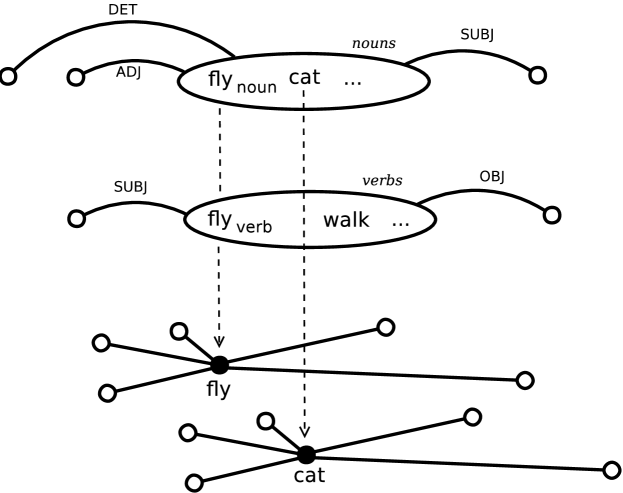
Figure 0.24: Polymorphism

This figure illustrates a polymorphic assignment for the word “fly”. It is split into two parts, the first, a noun, classed with other nouns, showing labeled connectors to determiners, adjectives, and a connector showing that nouns can act as the subject of a verb. The second class shows labeled connectors to subjects and objects, as is appropriate for transitive verbs. Underneath are the flattened raw seeds, showing the words “fly” and “cat” and the myriad of connectors on them. The flattened seeds cannot lead to grammatical linkages, as they mash together into one the connectors for different parts of speech.

 

The point of the figure is to illustrate that, although the “base graph” may not distinguish one variant of a vertex from another, it is important to discover, extract and represent this difference. The concept of “polymorphism” applies, because the base vertex behaves as one of several distinct types in practice. There are several ways the above diagram can be represented textually. As before, the Link Grammar-style notation is used, as it is fairly clear and direct. One representation would be to expose the polymorphism only in the connectors, and not in the base vertex label:

fly: (DET- & ADJ- & SUBJ+) or (SUBJ- & OBJ+);

A different possibility is to promptly split the vertex label into two, and ignore the subscript during the parsing stage:

fly.noun cat: (DET- & ADJ- & SUBJ+);

fly.verb walk: (SUBJ- & OBJ+);

Either way, the non-subscripted version of $fly$ behaves in a polymorphic fashion.

Note that the use of the notation “or” to disjoin the possibilities denotes a choice function, and not a boolean-or. That is, one can choose either one form, or the other; one cannot choose both. During the parse, both possibilities need to be considered, but only one selected in the end. This implies that at least some fragment of linear logic is at play, and not boolean logic. (this should be expanded upon in future drafts).

Similar concept: part of speech

It is tempting to identify the connectors DET, ADJ, SUBJ, OBJ in the diagrams above with “parts of speech”. This would be a mistake. In conventional grammatical analysis, there are half-a-dozen or a dozen parts of speech that are recognized: noun, verb, adjective, and so on. By contrast, these connector types indicate a grammatical role. That is, the disjunct SUBJ- & OBJ+ indicates a word that takes both a subject and an object: a transitive verb. That is, the disjunct is in essence a fine-grained part of speech, indicating not only verb-ness, but the specific type of verb-ness (transitive).

The Link Grammar English dictionary documents more than 100 connector types, these are subtyped, so that approximately 500 connectors might be seen. These connectors, when arranged into disjuncts, result in tens of thousands of disjuncts. That is, Link Grammar defines tens of thousands of distinct “parts of speech”. The can be thought of as parts of speech, but they are quite fine-grained, far more fine-grained than any text on grammar might ever care to list.

If one uses a technique, such as MST parsing[16], and then extracts disjuncts, one might observe more than 6 million disjuncts and 9 million seeds on a vocabulary of 140K words. These are, again, in the above technical sense, just “parts of speech”, but they are hyperfine-grained. The count is overwhelming. So, although it is techinically correct to call them “parts of speech”, it is a conceptual error to think of a class that has six million representatives as if it were a class with a dozen members.

Similar concept: skip-grams

The N-gram[11] and the more efficient skip-gram[17] models of semantic analysis provide somewhat similar tools for understanding connectivity, and differentiating different forms of connectivity. In a skip-gram model, one might extract two skip-grams from the above example sentences: “a fly landed” and “it fly home”. A clustering process, such as adagram or word2vec might be used to classify these two strings into distinct clusters, categorizing one with other noun-like words, and the other with verb-like words.

The N-gram or skip-gram technique works only for linear, sequenced data, which is sufficient for natural language, but cannot be employed in a generic non-ordered graphical setting. To make this clear: a seed representation for the above would be: “fly: a- landed+” indicating that the word “a” (written as the connector “a-”) comes sequentially before “fly”, while the word “landed” (written as the connector “landed+”) comes after. The other phrase has the representation “fly: it- home+”. These two can now be employed in a clustering algorithm, to determine whether they fall into the same, or into different categories. If one treats the skip-grams, and the seeds as merely two different representations of the same data, then applying the same algorithm to either should give essentially the same results.

The seed representation, however, is superior in two different ways. First, it can be used for non-sequential data. Second, by making clear the relationship between the vertex and its connectors, the connectors can be treated as “additional data”, tagging the vertex, carrying additional bits of information. That additional information is manifested from the overall graph structure, and is explicit. By contrast, untagged N-grams or untagged skip-grams leave all such structure implicit and hidden.

Polymorphism and semantics

The concept of polymorphism introduced above lays a foundation for semantics, for extracting meaning from graphs. This is already hinted at by the fact that any English-language dictionary will provide at least two different definitions for “fly”: one tagged as a noun, the other as a verb. The observation of hyperfine-grained parts of speech can push this agressively farther.

In a modern corpus of English, one might expect to observe the seeds “apple: green-” and “apple: iphone+”. The disjuncts “green-” and “iphone+” can be interpreted as a kind-of tag on the word “apple”. Since there are exactly two tags in this example, they can be viewed as supplying exactly one bit of additional information to the word “apple”. Effectively, a single apple has been split into two distinct apples. Are they really distinct, however? This can only be judged on the basis of some clustering algorithm that can assign tagged words to classes. Even very naive, unsophisticated algorithms might be expected to classify these two different kinds of apple into different classes; the extra bit of information carried by the disjunct is a bit of actual, usable information.

To summarize: the arrangement of vertexes into polymorphic seeds and sections enables the vertexes to be tagged with extra information. The tags are the connectors themselves: thier presence or absence carries information. That extra information can be treated as “semantic information”, identifying different types or kinds, rather than as purely syntactic information about arrangments and relationships.

Conclusion

This document presents a way of thinking about graphs that allows them to be decomposed into constituent parts fairly easily, and then brought together and reassembled in a coherent, syntactically correct fashion. It does so without having to play favorites among competing algorithmic approaches and scoring functions. It makes only one base assumption: that knowledge can be extracted at a symbolic level from pair-wise relationships between events or objects.

It touches briefly, all too briefly, on several closely-related topics, such as the application of category theory and type theory to the analysis of graph structure. These topics could be greatly expanded upon, possibly clarifying much of this content. It is now known to category theorists that there is a close relationship between categories, the internal languages that they encode, and that these are reflections of one another, reflecting through a theory of types. A reasonable but incomplete reference for some of this material is the HoTT book. It exposes types in greater detail, but does not cover the relationship between internal languages, parsing, and the modal logic descriptions of parsing. It is possible that there are texts in proof theory that cover these topics, but I am not aware of any.

This is a bit unfortunate, since I feel that much or most of what is written here is “well known” to computational proof theorists; unfortunately, that literature is not aimed at the data-mining and machine-learning crowd that this document tries to address. Additions, corrections and revisions are welcomed.

References

- [1] Daniel Sleator and Davy Temperley., Parsing English with a Link Grammar, Tech. rep., Carnegie Mellon University Computer Science technical report CMU-CS-91-196, 1991, URL http://arxiv.org/pdf/cmp-lg/9508004.
- [2] Bob Coecke, “Quantum Links Let Computers Read”, New Scientist, 2010, URL http://www.cs.ox.ac.uk/people/bob.coecke/NewScientist.pdf.
- [3] Dimitri Kartsaklis and Mehrnoosh Sadrzadeh, “A Study of Entanglement in a Categorical Framework of Natural Language”, Proceedings Quantum Physics and Logic, Electronic Proceedings in Theoretical Computer Science, 172, 2014, pp. 249–260, URL https://arxiv.org/abs/1405.2874.
- [4] John C. Baez and Mike Stay, “Physics, Topology, Logic and Computation: A Rosetta Stone”, Arxiv/abs/09030340, 2009, URL http://math.ucr.edu/home/baez/rosetta.pdf.
- [5] Daniel D. Sleator and Davy Temperley, “Parsing English with a Link Grammar”, in Proc. Third International Workshop on Parsing Technologies, 1993, pp. 277–292, URL http://www.cs.cmu.edu/afs/cs.cmu.edu/project/link/pub/www/papers/ps/LG-IWPT93.ps.
- [6] Hoifung Poon and Pedro Domingos, “Unsupervised Semantic Parsing”, in Proceedings of the 2009 Conference on Empirical Methods in Natural Language Processing, Association for Computational Linguistics, Singapore, 2009, pp. 1–10, URL http://www.aclweb.org/anthology/D09-1001.
- [7] J. Lambek, “On the calculus of syntactic types”, in Structure of Language and its Mathematical Aspects, America Methematical Society, 1961, pp. 166–178.
- [8] Solomon Marcus, Algebraic Linguistics; Analytical Models, 1967, URL https://monoskop.org/images/2/26/Marcus_Solomon_editor_Algebraic_Linguistics_Analytical_Models_1967.pdf.
- [9] Dimitri Kartsaklis, et al., “Reasoning about Meaning in Natural Language with Compact Closed Categories and Frobenius Algebras”, in Logic and Algebraic Structures in Quantum Computing, Cambridge University Press, 2013, URL https://www.cs.ox.ac.uk/files/5468/sadrzadeh_kartsaklis.pdf.
- [10] Mati Pentus, “Lambek Calculus and Formal Grammars”, American Mathematical Society Translations, 1998, URL http://lpcs.math.msu.su/~pentus/ftp/papers/ams.pdf.
- [11] Ronald Rosenfeld, “A Maximum Entropy Approach to Adaptive Statistical Language Modeling”, Computer Speech & Language, 10, 1996, pp. 187–228, URL https://www.cs.cmu.edu/\~roni/papers/me-csl-revised.pdf.
- [12] Robert B. Ash, Information Theory, Dover Publications, 1965.
- [13] David Eisenbud and Joe Harris, The Geometry of Schemes, Springer, 2000.
- [14] Saunders Mac Lane and Ieke Moerdijk, Sheaves in Geometry and Logic, Springer, 1992.
- [15] Bill Louw, “Truth, literary worlds and devices as collocation”, in Language and Computers, Corpora in the Foreign Language Classroom, edited by Luis Quereda Encarnación Hildalgo and Juan Santana, 2007, pp. 329–362, URL https://www.academia.edu/843973/Truth_literary_worlds_and_devices_as_collocation.
- [16] Deniz Yuret, Discovery of Linguistic Relations Using Lexical Attraction, PhD thesis, MIT, 1998, URL http://www2.denizyuret.com/pub/yuretphd.html.
- [17] David Guthrie, et al., “A Closer Look at Skip-gram Modelling”, Proceedings of the Fifth international Conference on Language Resources and Evaluation, 2006, URL https://homepages.inf.ed.ac.uk/ballison/pdf/lrec_skipgrams.pdf.