An Adaptive Weighted Deep Forest Classifier

Abstract

A modification of the confidence screening mechanism based on adaptive weighing of every training instance at each cascade level of the Deep Forest is proposed. The idea underlying the modification is very simple and stems from the confidence screening mechanism idea proposed by Pang et al. to simplify the Deep Forest classifier by means of updating the training set at each level in accordance with the classification accuracy of every training instance. However, if the confidence screening mechanism just removes instances from training and testing processes, then the proposed modification is more flexible and assigns weights by taking into account the classification accuracy. The modification is similar to the AdaBoost to some extent. Numerical experiments illustrate good performance of the proposed modification in comparison with the original Deep Forest proposed by Zhou and Feng.

Keywords: classification, random forest, deep forest,decision tree, class probability distribution, Adaboost

1 Introduction

One of the important developments in the field of ensemble-based models [5, 14, 22, 30] of the last years was a combination of several ensemble-based models, including random forests (RFs) [1] and the stacking, proposed by Zhou and Feng [31] and called the Deep Forest (DF) or gcForest. Its structure consists of layers similarly to a multi-layer neural network structure, but each layer in gcForest contains many RFs instead of neurons. gsForest can be regarded as an multi-layer ensemble of decision tree ensembles. As pointed out by Zhou and Feng [31], gcForest is much easier to train and can perfectly work when there are only small-scale training data in contrast to deep neural networks which require great effort in hyperparameter tuning and large-scale training data. A lot of numerical experiments provided by Zhou and Feng [31] illustrated that gcForest outperforms many well-known methods or comparable with existing methods.

One of the motivations for the DF development is to build deep models based on non-differentiable modules in contrast to deep neural networks which use backpropagation required differentiability. Another important motivation is to build deep models which require a small amount of training data due to a small number of training parameters. As a result, the DF taking into the above has exhibited high performance. This fact was a reason for developing new modifications of the DF and for applying it to several applications. In particular, Wang et al. [19] proposed to apply the deep forest to forecast the current health state or to diagnostic health monitoring. Yang et al. [25] applied the DF to solving the ship detection problem from thermal remote sensing imagery. Zheng et al. [29] considered application of the DF to the pedestrian detection problem in the framework of the extreme learning machine algorithms. The application of the DF to sentiment analysis was given in [15]. Xia et al. [24] used a DF modification to fuse multiple sources remotely sensed datasets, such as hyperspectral and Light Detection and Ranging (LiDAR)-derived digital surface model, where ensembles of Rotation Forests and RFs are introduced. Zhao et al. [28] proposed a deep forest-based protein location algorithm relying on sequence information.

Guo et al. [8] proposed a modification of the DF, called BCDForest, to classify cancer subtypes on small-scale biology datasets. The BCDForest uses a multi-class-grained scanning method to train multiple binary classifiers and a boosting strategy to emphasize more important features in cascade forests, thus to propagate the benefits of discriminative features among cascade layers to improve the classification performance. The same authors [7] used the DF in order to solve the same problem of the cancer subtype classification on gene expression data. Li et al. [10] applied the DF to hyperspectral image classification. Wen et al. [20] also proposed a modification of the DF for developing efficient recommendation methods. The modification is implemented by stacking Gradient Boosting Decision Trees in the DF cascade structures.

Some improvements have been proposed by Utkin and Ryabinin [17, 18, 16]. In particular, modifications of the DF for solving the weakly supervised and fully supervised metric learning problems were proposed in [18] and [16], respectively. A transfer learning model using the DF was presented in [17]. The main idea underlying the proposed modifications is to assign weights to decision trees in every RF in order to minimize the corresponding loss functions which depend on the problem solved. The weights are used to replace the standard averaging of the class probabilities for every instance and every decision tree with the weighted average. Yin et al. [26] introduced DF reinforcement learning applied to large-scale interconnected power systems for preventive strategy considering automatic generation control. Wu et al. [23] proposed an interesting modification of the DF, named the multi-features fusion cascade XGBoost, for human facial age estimation by means of a hierarchical regression approach. The modification uses the general idea of the DF, but it consists of the cascade XGBoost models instead of RFs. Another modification implemented and deployed the distributed version of the DF model for automatic detection of a cash-out fraud was provided by Zhang et al. [27]. Han et al. [9] proposed a combination of a convolution residual neural network with the DF for scene recognition. In fact, the DF in this combination aims to classify an extracted feature representation vector on the output of the residual neural network.

The same architecture of the cascade forest was proposed by Miller et al. [12]. However, this architecture differs from gcForest in using only class vectors at the next cascade levels without their concatenation with the original vector. Miller et al. [12] illustrated by numerical experiments that their approach is comparable to the approach [31]. We have to point out that the cascade structure with neural networks without backpropagation instead of forests was proposed by Hettinger et al. [2].

One of the crucial shortcomings of the DF is that it passes all training and testing instances through all levels of the cascade, leading to significant increase of time complexity. In order to overcome this difficulty, another improvement of the original DF was proposed by Pang et al. [13], which significantly reduces the training and testing times of forests at each level. According to the improvement, training examples with high confidence (the maximum value of the estimated class vector) directly pass to the final stage rather than passing through all the levels. Pang et al. [13] introduced a confidence screening mechanism in the general framework of the DF, which categorizes instances at every level of the cascade into two subsets: one is easy to predict; and the other is hard. The improvement opens a door for developing new models improving the DF.

Therefore, following the ideas of the DF improvement, we propose a new modification of the confidence screening mechanism based on adaptive weighing of every training instance at each cascade level depending on its mean class vector at the previous level. It is called the Adaptive Weighted Deep Forest (AWDF). Two ways are considered for applying weights. The first one is when the weighted instances are randomly chosen for training trees in accordance with their weights. This leads to reducing the set of “active” instances at every level of the forest cascade. The second way is to use weights in implementing a splitting rule for training the decision trees. The numerical experiments have shown that AWDF provides outperformed results.

The paper is organized as follows. A short description of gcForest proposed by Zhou and Feng [31] is given in Section 2. Section 3 provides the confidence screening mechanism proposed by Pang et al. [13]. AWDF algorithm is considered in Section 4. Numerical experiments with real data illustrating cases when the proposed AWDF outperforms gcForest are given in Section 5. Concluding remarks are provided in Section 6.

2 A short introduction to Deep Forests

One of the important peculiarities of gcForest is its cascade structure proposed by Zhou and Feng [31]. Every cascade is represented as an ensemble of decision tree forests. The cascade structure is a part of a total gcForest structure. It implements the idea of representation learning by means of the layer-by-layer processing of raw features. Each level of cascade structure receives feature information processed by its preceding level, and outputs its processing result to the next level. The architecture of the cascade proposed by Zhou and Feng [31] is shown in Fig. 1. It can be seen from the figure that each level of the cascade consists of two different pairs of RFs which generate 3-dimensional class vectors concatenated each other and with the original input. It should be noted that this structure of forests can be modified in order to improve the gcForest for a certain application. After the last level, we have the feature representation of the input feature vector, which can be classified in order to get the final prediction. The gcForest representational learning ability is enhanced by applying the second part of gcForest called as the so-called multi-grained scanning. The multi-grained scanning structure uses sliding windows to scan the raw features. Its output is a set of feature vectors produced by sliding windows of multiple sizes. We mainly pay attention to the first part of gcForest because our modification relates to the RFs.

Given an instance, each forest produces an estimate of a class distribution by counting the percentage of different classes of examples at the leaf node where the concerned instance falls into, and then averaging across all trees in the same forest as it is schematically shown in Fig. 2. The class distribution forms a class vector, which is then concatenated with the original vector to be input to the next level of cascade. The usage of the class vector as a result of the RF classification is very similar to the idea underlying the stacking algorithm [21] which trains the first-level learners using the original training dataset. Then the stacking algorithm generates a new dataset for training the second-level learner (meta-learner) such that the outputs of the first-level learners are regarded as input features for the second-level learner while the original labels are still regarded as labels of the new training data. In contrast to the standard stacking algorithm, gcForest simultaneously uses the original vector and the class vectors (meta-learners) at the next level of cascade by means of their concatenation. This implies that the feature vector is enlarged and enlarged after every cascade level. After the last level, we have the feature representation of the input feature vector, which can be classified in order to get the final prediction. Zhou and Feng [31] propose to use different forests at every level in order to provide the diversity which is an important requirement for the RF construction.

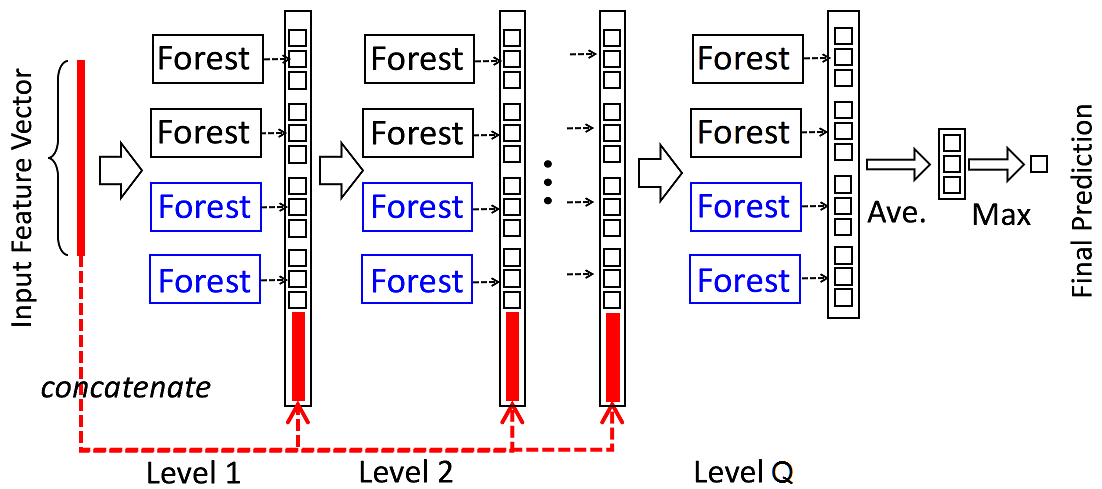
Figure 1: The architecture of the cascade forest [31]

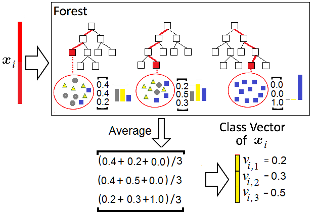
Figure 2: An illustration of the class vector generation by using average of the tree probability class vectors

3 The confidence screening mechanism

According to [13], the main idea underlying the confidence screening mechanism is that an instance is pushed to the next level of the cascade only if it is determined to require a higher level of learning; otherwise, it is predicted using the model at the current level.

We will consider the standard classification problem which can be formally written as follows. Given $n$ training instances $S=\{(\mathbf{x}_{1},y_{1}),(\mathbf{x}_{2},y_{2}),...,(\mathbf{x}_{n},y_{n})\}$, in which $\mathbf{x}_{i}\in\mathbb{R}^{m}$ represents a feature vector involving $m$ features and $y_{i}\in\{1,...,C\}$ represents the class of the associated instances, the task of classification is to construct an accurate classifier $c:$ $\mathbb{R}^{m}\rightarrow\{1,...,C\}$ that maximizes the probability that $c(\mathbf{x}_{i})=y_{i}$ for $i=1,...,n$.

A decision tree in every forest produces an estimate of the class probability distribution $\mathbf{p}=(p_{1},...,p_{C})$ by counting the percentage of different classes of training instances at the leaf node where the concerned instance falls into. Then the class probabilities $\mathbf{v}_{i}=\left(v_{i,1},...,v_{i,C}\right)$ of $\mathbf{x}_{i}$ for every RF are computed by averaging all class probability distributions $p$ across all trees as it is shown in Fig. 2, where we partly modify a picture from [31] in order to illustrate how elements of the class vector are derived as a simple sum.

Suppose that all RFs have the same number $T$ of decision trees, every cascade level contains $M$ RFs, and the number of cascade levels is $Q$. Then a current level of the cascade produces $M$ class vectors $\mathbf{v}_{i,1},...,\mathbf{v}_{i,M}$ which are then concatenated with the original vector $\mathbf{x}_{i}$ to be input to the next level of the cascade, i.e., the training set for the next level is defined as

$$S^{\ast}=\{((\mathbf{x}_{i},\mathbf{v}_{i,1},...,\mathbf{v}_{i,M}),y_{i}),i=1,...,n\}.$$

At level $q$, if the prediction confidence of one instance is larger than threshold $\eta_{q}$, then its final prediction is produced at the current level, otherwise it needs to go through the next level (and potentially all levels in the cascade). One of the ways to define the prediction confidence of instance $((\mathbf{x}_{i},\mathbf{v}_{i,1},...,\mathbf{v}_{i,M}),y_{i})$ is to find the mean vector of class probabilities, namely,

$$\mathbf{v}_{i}=\frac{1}{M}\sum_{k=1}^{M}\mathbf{v}_{i,k}.$$

Let us introduce the indicator $I$ defined as

$$I=\left\{\begin{array}[c]{cc}1,&\max(v_{i,1},...,v_{i,C})\geq\eta_{q},\\ 0,&\text{otherwise.}\end{array}\right.$$

The choice of the threshold $\eta_{q}$ is considered by Pang et al. [13] in detail, where $\eta_{q}$ at level $q$ is determined automatically based on the cross-validated error rate of all the training instances.

If the indicator $I$ is $0$, then the feature vector $\mathbf{x}_{i}$ has to go through the next level. If $I=1$, the final prediction is produced at the current level during testing such that

$$y_{i}=\arg_{c=1,...,C}\max v_{i,c}.$$

During training, we do not need to go through the next level if $I=1$ and

$$\arg_{c=1,...,C}\max v_{i,c}=y_{i},$$

otherwise the instance has to go through the next level $q+1$.

4 The adaptive weighted deep forest

We propose to assign a weight to every instance $\mathbf{x}_{i}$ at a current forest cascade level in accordance with its mean class vector $\mathbf{v}_{i}$ at the previous level. Let us introduce the vector $\mathbf{o}_{i}=(0,...,0,1_{y_{i}},0,...,0)$, where the index of the unit element is $y_{i}$. Then the weight $w_{i}$ is determined as a function $f$ of a distance between the mean vector of class probabilities $\mathbf{v}_{i}$ and the vector $\mathbf{o}_{i}$, denoted as $d(\mathbf{v}_{i},\mathbf{o}_{i})$. Suppose that we get the mean class vector $\mathbf{v}_{i}$ for instance $\mathbf{x}_{i}$ at the current level $q$. Then we can write the weight of instance $\mathbf{x}_{i}$ as

$$w_{i}=f(d(\mathbf{v}_{i},\mathbf{o}_{i})).$$

The weight $w_{i}$ is used for training RFs at the next level $q+1$. It is obvious that the function $f$ increases with $d(\mathbf{v}_{i},\mathbf{o}_{i})$. In particular, if instance $\mathbf{x}_{i}$ is correctly classified at level $q$ such that the distance $d(\mathbf{v}_{i},\mathbf{o}_{i})$ is $0$, then the weight $w_{i}$ has to be $0$. In this case, the instance is not used at the next level. In other words, due to the small weight, the instance $\mathbf{x}_{i}$ will have lesser chance to appear in the trees of the next level compared to other instances. If the distance is $1$ ($\mathbf{x}_{i}$ is totally incorrectly classified), then the weight $w_{i}$ has to be also $1$ or to have some maximal value. Simple examples of the function $f$ are $w_{i}=\left(d(\mathbf{v}_{i},\mathbf{o}_{i})\right)^{2}$ or $w_{i}=d(\mathbf{v}_{i},\mathbf{o}_{i})$. Moreover, the distance can be also differently taken. One of the most popular distances is Euclidean one, i.e., $d(\mathbf{v}_{i},\mathbf{o}_{i})=||\mathbf{v}_{i}-\mathbf{o}_{i}||_{2}$.

Another way for determining the weights is to consider the following function:

$$w_{i}=1-f(\mathbf{v}_{i}\cdot\mathbf{o}_{i}^{\mathrm{T}}).$$

In this case, we analyze only a probability of the class $y_{i}$, i.e., $v_{i,y_{i}}$. If this probability of an instance is close to $1$ (correct classification), then the corresponding weight of the instance is close to $0$. If the probability of the instance is close to $0$ (incorrect classification), then the corresponding weight is close to $1$. A simplest case is $w_{i}=1-\mathbf{v}_{i}\cdot\mathbf{o}_{i}^{\mathrm{T}}$. This definition of weights almost coincides with the rule for decision about going the instance through the next level in the confidence screening mechanism (see the previous section).

It should be noted that the normalized weights $w_{1},...,w_{n}$ define a probability distribution on instances in the training data, which can be used for building decision trees of a RF.

We define two strategies for using the weights. In accordance with the first strategy, we randomly draw instances from the training set with replacement in accordance with this probability distribution. If the weight of the $i$-th instance is very close to $0$, it does not take part in building decision trees. In other words, instances with a high prediction confidence are predicted using the model at the current level.

In addition to the above weighted procedure, we can also introduce a threshold $\eta_{q}$ to compare it with the value $1-w_{i}$. If the $1-w_{i}\geq\eta_{q}$, then the corresponding instance is predicted by using the model at current level. In sum, the number of instances for training are reduced at every level simplifying the whole training process. However, if the training set is imbalanced, then the number of randomly drawn instances of a class may be very small to be used for training.

The proposed approach is intuitively very close to the AdaBoost algorithm [6], where instances from a training set are drawn for classification from an iteratively updated sample distribution defined on elements of the training set. Every level of the DF can be viewed as an iteration in AdaBoost. The sample distribution ensures that instances misclassified by the previous classifier (at the previous iteration) are more likely to be included in the training data of the next classifier. In each iteration, the weights of all misclassified instances are increased while the weights of correctly classified examples are decreased.

According to the second strategy, we apply the procedure of direct use of the weights during learning in a splitting rule, which is implemented in many versions of the decision tree algorithms, for example, in C4.5 and CART. In particular, the weights and the entropy measure are combined in the splitting rule. The weights are again viewed as probabilities of instances and used in definition of the entropy measure. This strategy does not simplify the whole deep forest training process because all instances are used for training the trees. However, the problem of a lack of instances of a certain class at some level is avoided in this case.

5 Numerical experiments

In order to illustrate AWDF, we investigate the model for datasets from UCI Machine Learning Repository [4]. Table 1 is a brief introduction about these data sets, while more detailed information can be found from, respectively, the data resources. Table 1 shows the number of features $m$ for the corresponding dataset, the number of training instances $n$ and the number of classes $C$. We also use the IMDB dataset [11] for the sentiment classification, which consists of 25000 movie reviews for training and 25000 for testing. The reviews are represented by tf-idf features. The IMDB dataset is available at http://ai.stanford.edu/~amaas/data/sentiment.

AWDF uses a software in Python which implements gcForest and is available at http://lamda.nju.edu.cn/code_gcForest.ashx. AWDF has the same cascade structure as the standard gcForest described in [31] (two completely-random tree forests and two random forests at every level, completely-random trees are generated by randomly selecting a feature for split at each node of the tree). The forest cascade is used for numerical experiments without the Multi-Grained Scanning part of gcForest. Accuracy measure $A$ used in numerical experiments is the proportion of correctly classified cases on a sample of data. To evaluate the average accuracy, we perform a cross-validation with $50$ repetitions, where in each run, we randomly select $n_{\text{tr}}=4n/5$ training data and $n_{\text{test}}=n/5$ testing data. We apply the second strategy to training RFs by using the weighted instances because we are interesting in increasing the accuracy of AWDF, but not training or testing time. However, we also provide results for the first strategy.

Table 1: A brief introduction about data sets

Data set	Abbreviation	$m$	$n$	$C$
Adult Income	Adult	$14$	$48842$	$2$
Car	Car	$6$	$1728$	$4$
Diabetic Retinopathy	Diabet	$20$	$1151$	$2$
EEG Eye State	EEG	$15$	$14980$	$2$
Haberman’s Breast Cancer Survival	Haberman	$3$	$306$	$2$
Ionosphere	Ion	$34$	$351$	$2$
Seeds	Seeds	$7$	$210$	$3$
Seismic Mining	Seismic	$19$	$2584$	$2$
Teaching Assistant Evaluation	TAE	$5$	$151$	$3$
Tic-Tac-Toe Endgame	TTTE	$9$	$958$	$2$
Website Phishing	Website	$30$	$2456$	$3$
Wholesale Customer Region	WCR	$8$	$440$	$3$
Letter	Letter	$16$	$20000$	$26$
Yeast	Yeast	$8$	$1484$	$10$
Nursery	Nursery	$8$	$12960$	$5$
Ecoli	Ecoli	$8$	$336$	$8$
Dermatology	Dermatology	$33$	$366$	$6$
IMDB	IMDB	$5000$	$50000$	$2$

First of all, our aim is to compare AWDF with gcForest and to consider different cases of the weight function $f$. We denote $w_{i}=1-(\mathbf{v}_{i}\cdot\mathbf{o}_{i}^{\mathrm{T}})^{2}$ as $1-w^{2}$; $w_{i}=1-(\mathbf{v}_{i}\cdot\mathbf{o}_{i}^{\mathrm{T}})^{1/2}$ as $1-w^{1/2}$; $w_{i}=1-(\mathbf{v}_{i}\cdot\mathbf{o}_{i}^{\mathrm{T}})$ as $1-w$; $w_{i}=||\mathbf{v}_{i}-\mathbf{o}_{i}||_{2}$ (Euclidean distance) as $L_{2}$. Numerical results of comparison of gcForest (gcF) and four cases of the weight definition are shown in Table 2, where the first column contains abbreviations of the tested data sets, the second column is the accuracy measure by using gcForest, other columns correspond to the accuracy measures of AWDF by different functions of weights. It should be noted that the largest values of the accuracy measures obtained by different numbers of trees are shown in Table 2. It can be seen from Table 2 that at least one of the cases of the proposed AWDF outperforms gcForest for most considered data sets. The best performance on each dataset is shown in bold. We note that our method yields the best accuracy on 16 out of 18 datasets tested.

We can also conclude from Table 2 that there is no the best choice of the weight function for all datasets. Though, we can also see that the function $w_{i}=1-(\mathbf{v}_{i}\cdot\mathbf{o}_{i}^{\mathrm{T}})^{1/2}$ provides the largest number of the best results. This function makes weights to be close to $0$ if an instance is correctly classified. At the same time, the “bad” instances have weights close to $1$, and they introduce a large impact in computing the splitting rule. In contrast to this function, function $1-(\mathbf{v}_{i}\cdot\mathbf{o}_{i}^{\mathrm{T}})^{2}$ shows worse results. This is due to the fact that the resulting weights are close to $0.5$. As a result, the difference between weights of correctly and incorrectly classified instances is smaller, and the separation effect is reduced.

Table 2: Accuracy measures gcForest and four cases of the weight function for the second strategy of using weights

Data set	gcF	$1-w^{2}$	$1-w^{1/2}$	$L_{2}$	$1-w$
Adult	$86.12$	$86.20$	$86.26$	$86.11$	$\mathbf{86.30}$
Car	$98.28$	$98.42$	$\mathbf{98.74}$	$98.45$	$98.51$
Diabet	$69.05$	$69.06$	$\mathbf{69.69}$	$69.16$	$69.13$
EEG	$95.75$	$95.82$	$\mathbf{96.16}$	$95.74$	$95.94$
Haberman	$74.15$	$73.90$	$\mathbf{74.77}$	$74.09$	$73.65$
Ion	$94.32$	$94.32$	$94.37$	$94.26$	$\mathbf{94.64}$
Seeds	$93.17$	$\mathbf{93.62}$	$\mathbf{93.62}$	$93.08$	$92.72$
Seismic	$93.50$	$93.63$	$93.53$	$\mathbf{93.67}$	$93.61$
TAE	$52.76$	$53.76$	$55.14$	$55.26$	$\mathbf{55.76}$
TTTE	$99.03$	$99.09$	$\mathbf{99.11}$	$\mathbf{99.11}$	$98.99$
Website	$90.15$	$90.45$	$\mathbf{90.59}$	$90.00$	$90.25$
WCR	$\mathbf{72.81}$	$72.47$	$72.64$	$72.29$	$72.47$
Letter	$97.14$	$97.06$	$97.08$	$\mathbf{97.18}$	$97.07$
Yeast	$63.03$	$\mathbf{62.92}$	$63.26$	$62.56$	$62.81$
Nursery	$66.40$	$66.49$	$66.56$	$\mathbf{66.67}$	$66.28$
Ecoli	$\mathbf{89.15}$	$85.27$	$87.50$	$89.14$	$84.52$
Dermatology	$58.10$	$59.47$	$59.47$	$59.21$	$\mathbf{60.30}$
IMDB	$88.74$	$89.21$	$\mathbf{89.44}$	$88.95$	$89.35$

In order to formally show the outperformance of the proposed AWDF, we apply the $t$-test which has been proposed and described by Demsar [3] for testing whether the average difference in the performance of two classifiers AWDF and gcForest is significantly different from zero. We can use the differences between accuracy measures of AWDF and gcForest, and then to compare them with $0$. The $t$ statistics in this case is distributed according to the Student distribution with $18-1$ degrees of freedom. The results of computing the $t$ statistics for the difference between the best value of AWDF and gcForest are the p-values denoted as $p$ and the $95\%$ confidence interval for the mean $0.557$, which are $p=0.0083$ and $[0.164,0.951]$, respectively. The $t$-test demonstrates the clear outperforming of the proposed model in comparison with gcForest.

In order to investigate how the accuracy measures depend on the number of decision trees in the RF, we depict the corresponding dependencies in Figs. 3-11. We compare gcForest and AWDF by four different weight functions. We again can see from Figs. 3-11 that AWDF outperforms gcForest for all datasets. Table 2 is composed from largest values of accuracy measures given in Figs. 3-11.

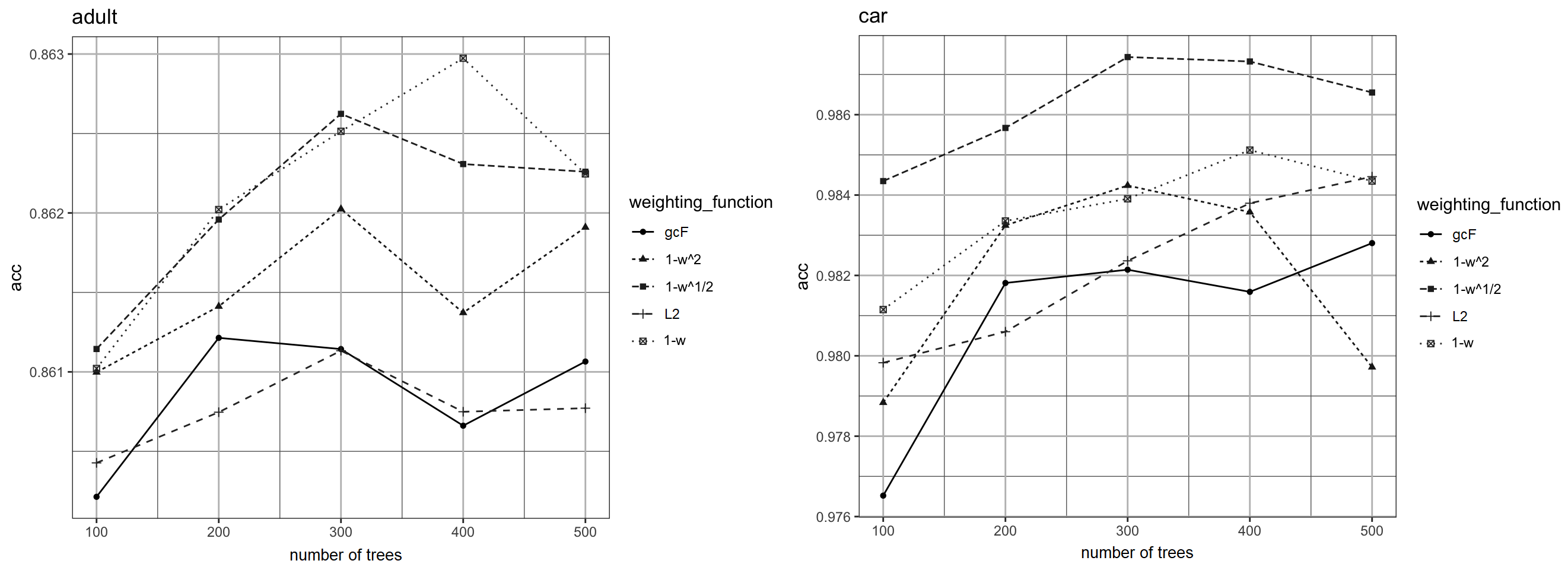
Figure 3: Accuracy measures as a function of the number of trees for the Adult and Car datasets

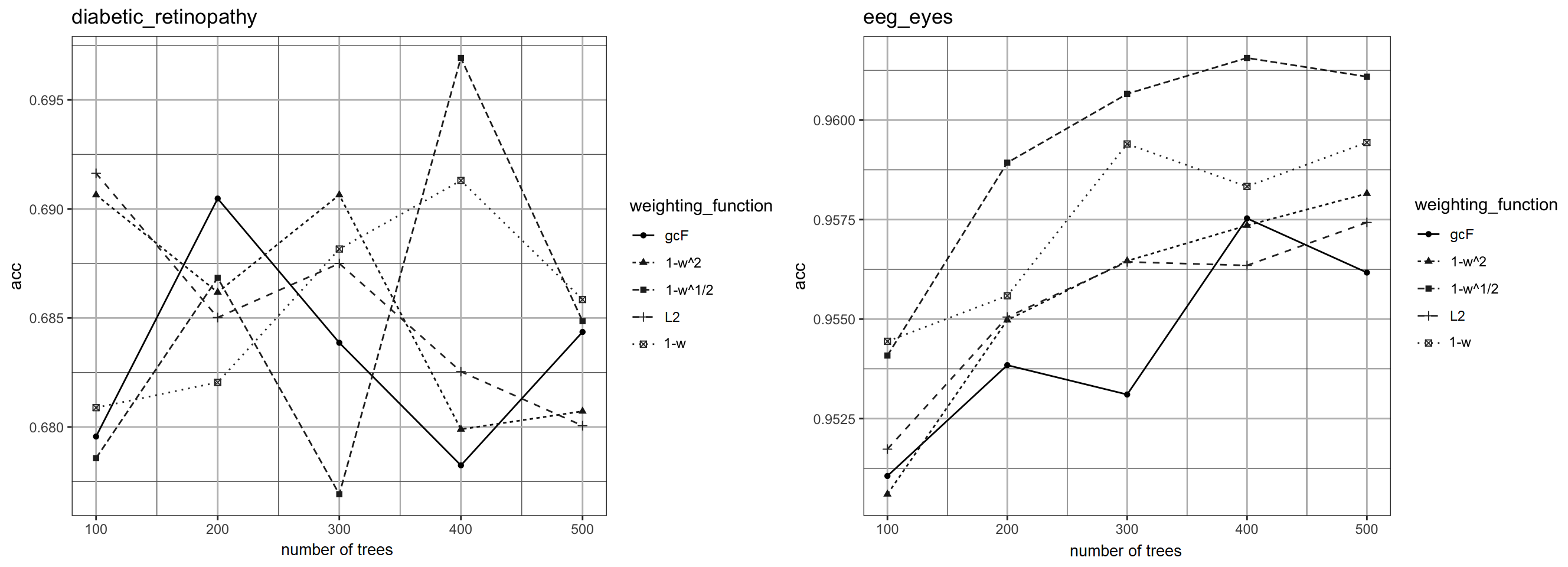
Figure 4: Accuracy measures as a function of the number of trees for the Diabetic and EEG datasets

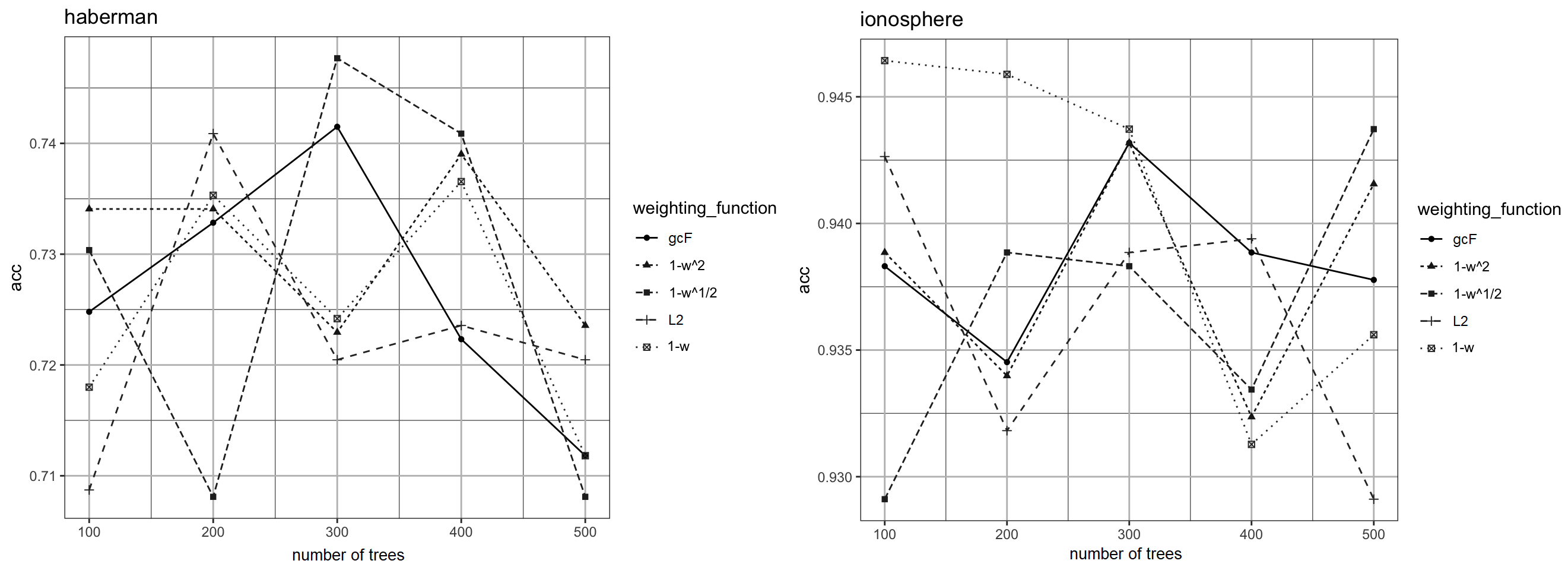
Figure 5: Accuracy measures as a function of the number of trees for the Haberman and Ionosphere datasets

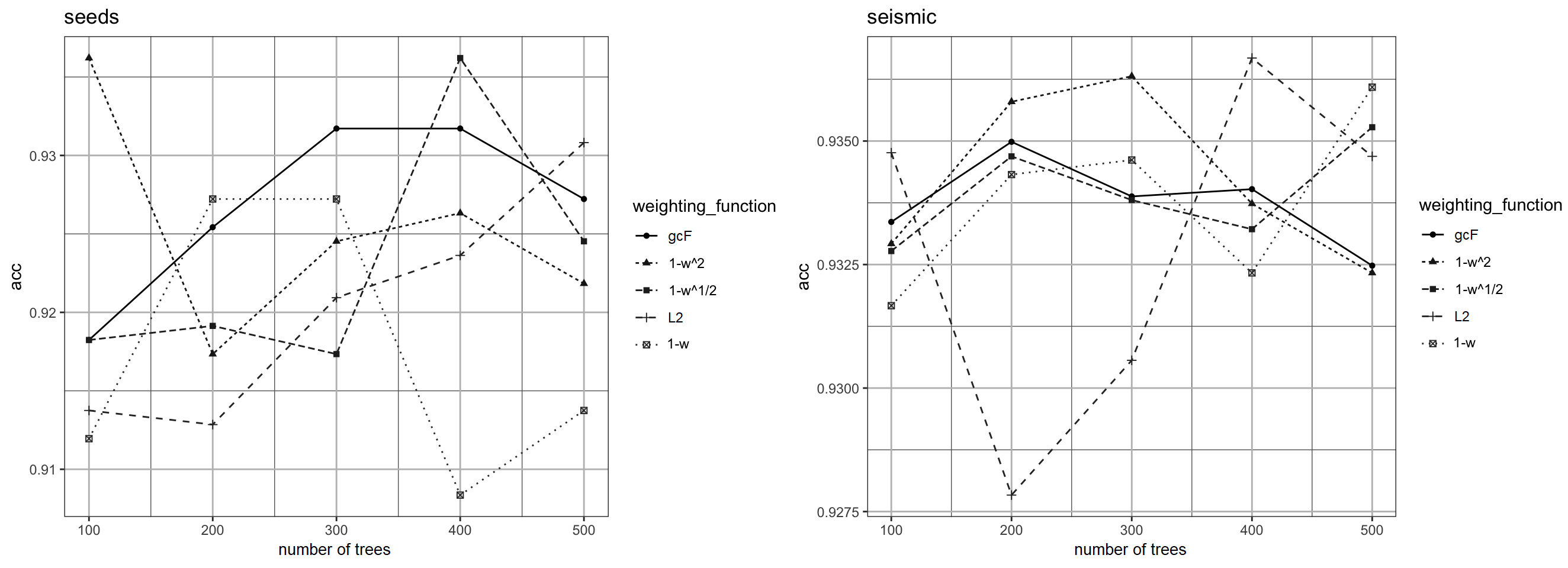
Figure 6: Accuracy measures as a function of the number of trees for the Seeds and Seismic datasets

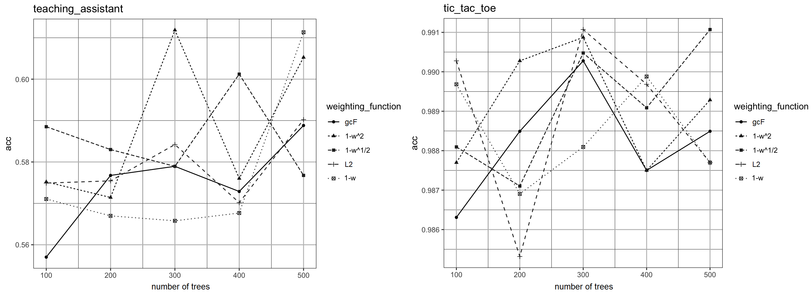
Figure 7: Accuracy measures as a function of the number of trees for the TAE and TTTE datasets

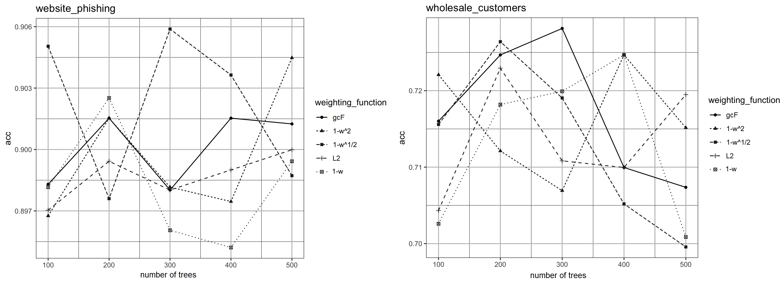
Figure 8: Accuracy measures as a function of the number of trees for the Website and WCR datasets

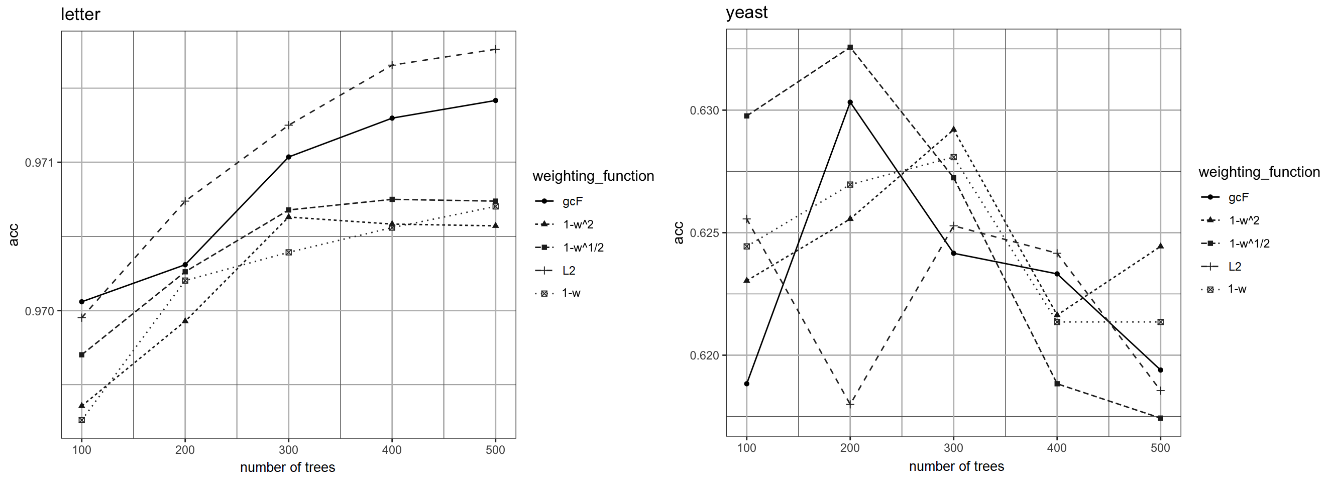
Figure 9: Accuracy measures as a function of the number of trees for the Letter and Yeast datasets

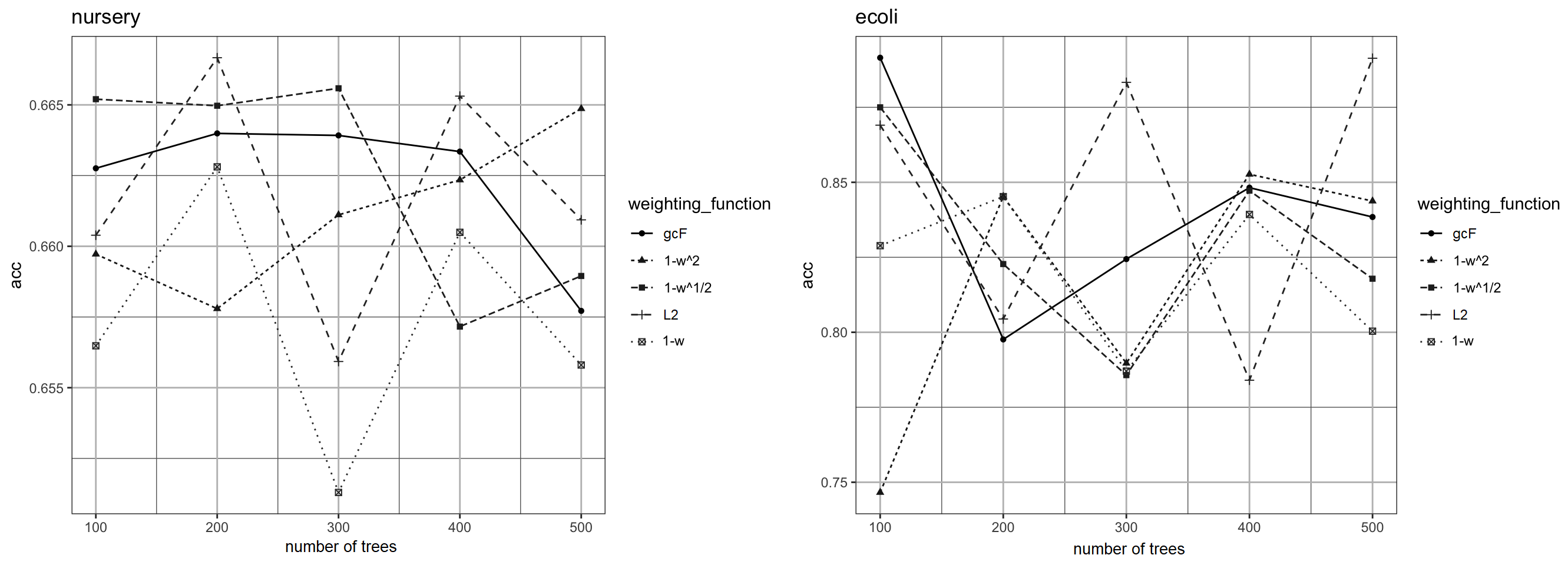
Figure 10: Accuracy measures as a function of the number of trees for the Nursery and Ecoli datasets

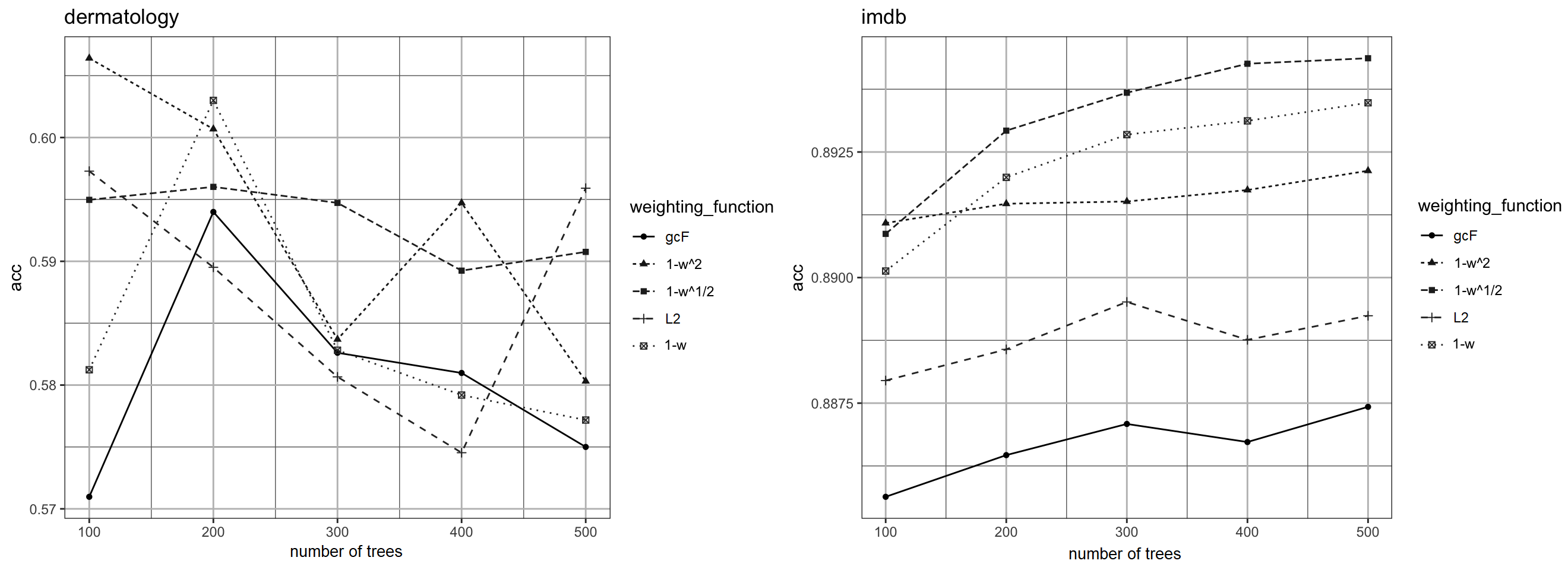
Figure 11: Accuracy measures as a function of the number of trees for the Dermatology and IMDB datasets

Tabl. 3 shows accuracy measures in accordance with the first strategy of using weights when we randomly draw instances from the training set with replacement in accordance with the probability distribution corresponding to the weights. One can see from Tabl. 3 that AWDF is comparable with gcForest, but it yields the best accuracy on 7 out of 15 datasets tested. This can be explained by the fact that we significantly reduce the training time by removing a large part of instances from the training process after the first cascade level. Perhaps, a more fine tuning of AWDF (choice of an appropriate function of weights) may improve the classification results.

Table 3: Accuracy measures gcForest and four cases of the weight function for the first strategy of using weights

Data set	gcF	$1-w^{2}$	$1-w^{1/2}$	$L_{2}$	$1-w$
Adult	$\mathbf{86.12}$	$85.98$	$85.72$	$85.95$	$85.84$
Car	$98.28$	$98.16$	$98.27$	$97.88$	$\mathbf{98.39}$
Diabet	$69.05$	$68.57$	$\mathbf{69.62}$	$68.25$	$68.38$
EEG	$\mathbf{95.75}$	$94.92$	$95.29$	$94.70$	$95.13$
Haberman	$\mathbf{74.15}$	$72.17$	$73.22$	$73.35$	$72.97$
Ion	$\mathbf{94.32}$	$93.94$	$94.10$	$94.21$	$93.78$
Seeds	$\mathbf{93.17}$	$92.90$	$92.09$	$92.45$	$91.88$
Seismic	$93.50$	$\mathbf{93.79}$	$\mathbf{93.79}$	$93.60$	$93.47$
TAE	$52.76$	$51.88$	$52.38$	$53.63$	$\mathbf{53.65}$
TTTE	$\mathbf{99.03}$	$98.33$	$98.81$	$98.41$	$98.63$
Website	$\mathbf{90.15}$	$90.03$	$88.92$	$89.86$	$89.67$
WCR	$72.81$	$71.52$	$72.12$	$72.68$	$\mathbf{73.33}$
Letter	$\mathbf{97.14}$	$96.47$	$96.59$	$96.40$	$96.55$
Nursery	$66.40$	$\mathbf{66.55}$	$66.31$	$66.38$	$66.44$
Dermatology	$58.10$	$\mathbf{65.22}$	$60.68$	$65.21$	$58.15$

We again apply the $t$-test for the difference between accuracy measures of gcForest and AWDF. The results of computing the $t$ statistics for the difference between the best value of AWDF and gcForest are the p-values denoted as $p$ and the $95\%$ confidence interval for the mean $0.465$, which are $p=0.3577$ and $[-0.584,1.515]$, respectively. The $t$-test demonstrates that there is not significant difference between accuracy measures of gcForest and AWDF when we apply the first strategy of using weights.

Examples of the dependencies of the accuracy measures on the number of decision trees in every RF for the first strategy of using weights are shown in Fig. 12. We clearly see from Fig. 12 that AWDF does not outperform gcForest.

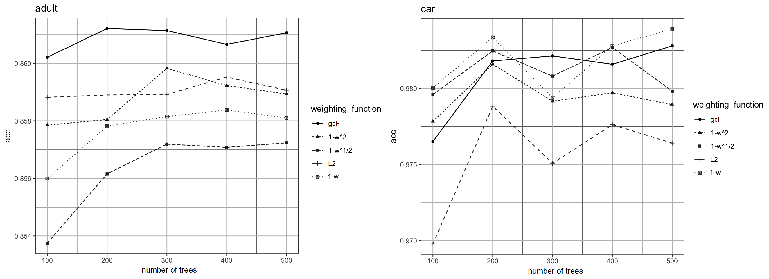
Figure 12: Accuracy measures as a function of the number of trees for the Adult and Car datasets for the first strategy of using weights

It follows from the above results that the second strategy of using weights provides better accuracies in comparison with the first strategy.

Let us consider how the introduction of threshold $\eta_{q}$ for AWDF impacts on the accuracy measures. Tabl. 4 shows accuracy measures in accordance with the second strategy of using weights by $\eta_{q}=0.95$. One can see from Tabl. 4 that AWDF yields the best accuracy on 13 out of 16 datasets tested. At the same time, we have to note that the training time by using the threshold is significantly reduced. Fig. 13 shows examples of the training time as a function of the number of trees. One can see that the training time is reduced for AWDF in comparison with gcForest.

Table 4: Accuracy measures gcForest and four cases of the weight function for the second strategy of using weights and threshold $\eta_{q}=0.95$

Data set	gcF	$1-w^{2}$	$1-w^{1/2}$	$L_{2}$	$1-w$
Adult	$86.12$	$86.09$	$86.10$	$86.04$	$\mathbf{86.13}$
Car	$\mathbf{98.28}$	$96.46$	$96.83$	$96.16$	$96.54$
Diabet	$69.05$	$69.71$	$69.71$	$\mathbf{69.92}$	$69.84$
EEG	$\mathbf{95.75}$	$92.54$	$92.44$	$92.45$	$92.47$
Haberman	$74.15$	$74.52$	$73.47$	$73.10$	$\mathbf{73.59}$
Ion	$94.32$	$\mathbf{95.18}$	$94.26$	$94.91$	$93.51$
Seeds	$93.17$	$93.26$	$92.90$	$\mathbf{93.71}$	$93.17$
Seismic	$93.50$	$93.37$	$93.68$	$\mathbf{93.73}$	$93.54$
TAE	$52.76$	$53.26$	$\mathbf{54.39}$	$53.88$	$53.38$
TTTE	$99.03$	$97.42$	$\mathbf{97.62}$	$97.20$	$97.22$
Website	$90.15$	$90.27$	$90.32$	$90.25$	$\mathbf{90.52}$
WCR	$72.81$	$72.60$	$\mathbf{72.94}$	$72.16$	$72.21$
Letter	$\mathbf{97.14}$	$96.35$	$96.35$	$96.35$	$96.35$
Yeast	$63.03$	$62.97$	$63.00$	$\mathbf{63.11}$	$63.04$
Nursery	$66.40$	$65.24$	$65.51$	$66.13$	$\mathbf{65.95}$
Dermatology	$58.10$	$\mathbf{58.98}$	$58.39$	$58.64$	$57.99$

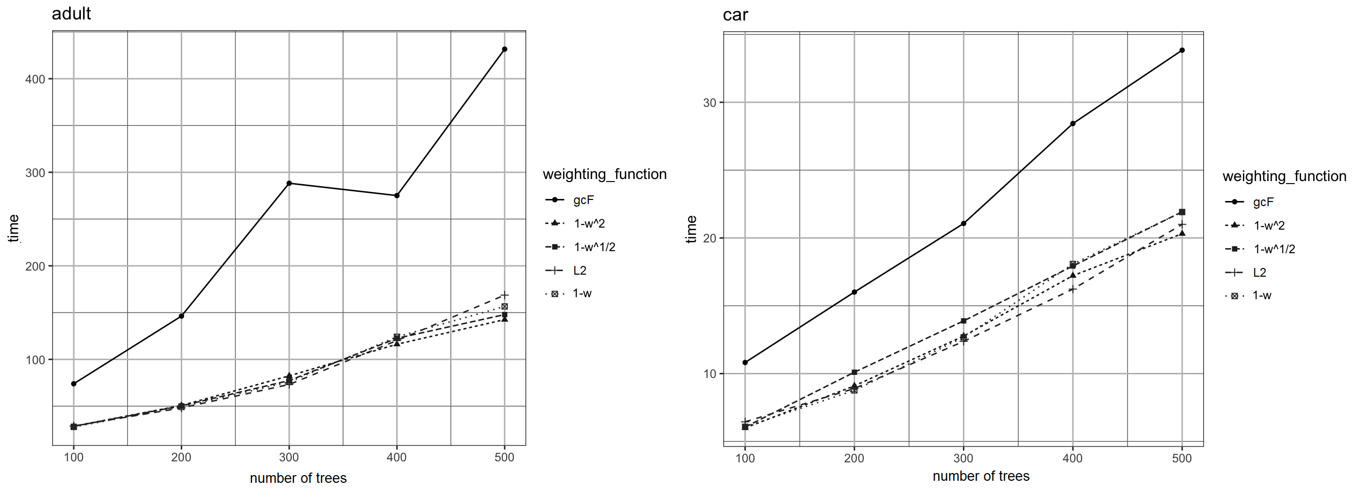
Figure 13: The training time of classifiers as a function of the number of trees for the Adult and Car datasets for the second strategy of using weights and threshold $\eta_{q}=0.95$

6 Conclusion

The proposed modification of the confidence screening mechanism based on adaptive weighing of every training instance at each cascade level of DF has demonstrated good performance in comparison with gcForest by means of numerical experiments on several datasets. Its implementation is very simple and is similar to the well-known AdaBoost model in a sense that it updates weights of training instances at each level of the forest cascade.

The idea underlying AWDF is very simple and its implementation does not require a large additional time because weights are computed in a simple way without solving optimization problems.

Similarly to gcForest, the main advantage of AWDF is that it opens a door for developing many new adaptive weight models which could take into account different rules for updating and assigning the weights to instances at different levels of the cascade. Moreover, the weights can be assigned in accordance with the problem solved, for example, for improving the DF transfer learning algorithms, for improving the distance metric learning algorithms, etc. In other words, the weights can control the DF models. The development of the corresponding algorithms is a problem for further research.

It should be noted that the proposed approach for adaptive weighing of every training instances at each cascade level can be simply extended on cases when classifiers different from RFs are used at every level because there are weighted versions of the most classifiers. The choice of optimal structures is also a problem for further research.

References

- [1] L. Breiman. Bagging predictors. Machine Learning, 24(2):123–140, 1996.
- [2] T. Christensen C. Hettinger, B. Ehlert, J. Humpherys, T. Jarvis, and S. Wade. Forward thinking: Building and training neural networks one layer at a time. arXiv:1706.02480v1, Jun 2017.
- [3] J. Demsar. Statistical comparisons of classifiers over multiple data sets. Journal of Machine Learning Research, 7:1–30, 2006.
- [4] Dua Dheeru and Efi Karra Taniskidou. UCI machine learning repository, 2017.
- [5] A.J. Ferreira and M.A.T. Figueiredo. Boosting algorithms: A review of methods, theory, and applications. In C. Zhang and Y. Ma, editors, Ensemble Machine Learning: Methods and Applications, pages 35–85. Springer, New York, 2012.
- [6] Y. Freund and R.E. Schapire. A decision theoretic generalization of on-line learning and an application to boosting. Journal of Computer and System Sciences, 55(1):119–139, 1997.
- [7] Y. Guo, S. Liu, Z. Li, and X. Shang. Towards the classification of cancer subtypes by using cascade deep forest model in gene expression data. In 2017 IEEE International Conference on Bioinformatics and Biomedicine (BIBM), pages 1664–1669, Nov 2017.
- [8] Y. Guo, S. Liu, Z. Li, and X. Shang. BCDForest: a boosting cascade deep forest model towards the classification of cancer subtypes based on gene expression data. BMC Bioinformatics, 19(Suppl 5):118:1–13, 2018.
- [9] M. Han, S. Li, X. Wan, and G. Liu. Scene recognition with convolutional residual features via deep forest. In 2018 3rd IEEE International Conference on Image, Vision and Computing, pages 178–182. IEEE, 2018.
- [10] M. Li, N. Zhang, B. Pan, S. Xie, X. Wu, and Z. Shi. Hyperspectral image classification based on deep forest and spectral-spatial cooperative feature. In Image and Graphics. ICIG 2017, volume 10668 of Lecture Notes in Computer Science, pages 325–336, Cham, 2017. Springer.
- [11] A.L. Maas, R.E. Daly, P.T. Pham, D. Huang, A.Y. Ng, and C. Potts. Learning word vectors for sentiment analysis. In Proceedings of the 49th annual meeting of the association for computational linguistics: Human language technologies, volume 1, pages 142–150. Association for Computational Linguistics.
- [12] K. Miller, C. Hettinger, J. Humpherys, T. Jarvis, and D. Kartchner. Forward thinking: Building deep random forests. arXiv:1705.07366, 20 May 2017.
- [13] M. Pang, K.M. Ting, P. Zhao, and Z.-H. Zhou. Improving deep forest by confidence screening. In Proceedings of the 18th IEEE International Conference on Data Mining (ICDM’18), pages 1–6, Singapore, 2018.
- [14] L. Rokach. Ensemble-based classifiers. Artificial Intelligence Review, 33(1-2):1–39, 2010.
- [15] K.P. S, S. Kapoor, K.S. Oza, and R.K. Kamat. A comprehensive study on sentiment analysis using deep forest. International Journal of Computer Sciences and Engineering, 6(8):115–123, 2018.
- [16] L.V. Utkin and M.A. Ryabinin. Discriminative metric learning with deep forest. arXiv:1705.09620v1, May 2017.
- [17] L.V. Utkin and M.A. Ryabinin. A deep forest for transductive transfer learning by using a consensus measure. In A. Filchenkov, L. Pivovarova, and J. Zizka, editors, Artificial Intelligence and Natural Language. AINL 2017, volume 789 of Communications in Computer and Information Science, pages 194–208. Springer, Cham, 2018.
- [18] L.V. Utkin and M.A. Ryabinin. A Siamese deep forest. Knowledge-Based Systems, 139:13–22, 2018.
- [19] C. Wang, N. Lu, Y. Cheng, and B. Jiang. Deep forest based multivariate classification for diagnostic health monitoring. In 2018 Chinese Control And Decision Conference (CCDC), pages 6233–6238, Shenyang, 2018.
- [20] H. Wen, J. Zhang, Q. Lin, K. Yang, T. Jin, F. Lv, X. Pan, P. Huang, and Z.-J. Zha. Multi-level deep cascade trees for conversion rate prediction. arXiv:1805.09484, May 2018.
- [21] D.H. Wolpert. Stacked generalization. Neural networks, 5(2):241–259, 1992.
- [22] M. Wozniak, M. Grana, and E. Corchado. A survey of multiple classifier systems as hybrid systems. Information Fusion, pages 3–17, 2014.
- [23] T. Wu, Y. Zhao, L. Liu, H. Li, W. Xu, and C. Chen. A novel hierarchical regression approach for human facial age estimation based on deep forest. In 2018 IEEE 15th International Conference on Networking, Sensing and Control (ICNSC), pages 1–6, Zhuhai, 2018. IEEE.
- [24] J. Xia, Z. Ming, and A. Iwasaki. Multiple sources data fusion via deep forest. In IGARSS 2018 - 2018 IEEE International Geoscience and Remote Sensing Symposium, pages 1722–1725, Valencia, Spain, 2018. IEEE.
- [25] F. Yang, Q. Xu, B. Li, and Y. Ji. Ship detection from thermal remote sensing imagery through region-based deep forest. IEEE Geoscience and Remote Sensing Letters, PP(99):1–5, 2018.
- [26] L. Yin, L. Zhao, T. Yu, and X. Zhang. Deep forest reinforcement learning for preventive strategy considering automatic generation control in large-scale interconnected power systems. Applied Sciences, 8(11):1–19, 2018. 2185.
- [27] Y.-L. Zhang, J. Zhou, W. Zheng, J. Feng, L. Li, Z. Liu, M. Li, Z. Zhang, C. Chen, X. Li, and Z.-H. Zhou. Distributed deep forest and its application to automatic detection of cash-out fraud. arXiv:1805.04234v2, May 2018.
- [28] L. Zhao, J. Wang, M.M. Nabil, and J. Zhang. Deep forest-based prediction of protein subcellular localization. Current Gene Therapy, 18(5):268–274, 2018.
- [29] W. Zheng, S. Cao, X. Jin, S. Mo, H. Gao, Y. Qu, C. Zheng, S. Long, J. Shuai, Z. Xie, W. Jiang, H. Du, and Y. Zhu. Deep forest with local experts based on elm for pedestrian detection. In Advances in Multimedia Information Processing – PCM 2018, volume 2 of Lecture Notes in Computer Science, pages 803–814. Springer International Publishing, 2018.
- [30] Z.-H. Zhou. Ensemble Methods: Foundations and Algorithms. CRC Press, Boca Raton, 2012.
- [31] Z.-H. Zhou and J. Feng. Deep forest: Towards an alternative to deep neural networks. In Proceedings of the 26th International Joint Conference on Artificial Intelligence (IJCAI’17), pages 3553–3559, Melbourne, Australia, 2017. AAAI Press.