Fractional Burgers models in
creep and stress relaxation tests

Abstract

Classical and thermodynamically consistent fractional Burgers models are examined in creep and stress relaxation tests. Using the Laplace transform method, the creep compliance and relaxation modulus are obtained in integral form, that yielded, when compared to the thermodynamical requirements, the narrower range of model parameters in which the creep compliance is a Bernstein function while the relaxation modulus is completely monotonic. Moreover, the relaxation modulus may even be oscillatory function with decreasing amplitude. The asymptotic analysis of the creep compliance and relaxation modulus is performed near the initial time-instant and for large time as well.

Key words: thermodynamically consistent fractional Burgers models, creep compliance and relaxation modulus, Bernstein and completely monotonic functions

1 Introduction

The classical Burgers model

$$\left(1+a_{1}\frac{\mathrm{d}}{\mathrm{d}t}+a_{2}\frac{\mathrm{d}^{2}}{\mathrm{d}t^{2}}\right)\sigma\left(t\right)=\left(b_{1}\frac{\mathrm{d}}{\mathrm{d}t}+b_{2}\frac{\mathrm{d}^{2}}{\mathrm{d}t^{2}}\right)\varepsilon\left(t\right),$$ (1)

where $\sigma$ and $\varepsilon$ denote stress and strain, that are functions of time $t>0,$ while $a_{1},a_{2},b_{1},b_{2}>0$ are model parameters, see [9, 12], is obtained using the rheological representation shown in Figure 1. Thermodynamical constraints

$$\frac{a_{2}}{a_{1}}\leq\frac{b_{2}}{b_{1}}\leq a_{1}$$ (2)

on model parameters appearing in the classical Burgers model (1) are derived in [16] by requiring non-negativity of the storage and loss modulus that is obtained as a consequence of the dissipativity inequality in the steady state regime, see [5].

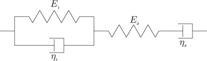
Figure 1: Rheological representation of the classical Burgers model.

The fractional generalization of Burgers model is derived in [16] by considering the Scott-Blair (fractional) element instead of the dash-pot element in the rheological representation from Figure 1, with the orders of fractional differentiation corresponding to the fractional elements and their sums being replaced by the arbitrary orders of fractional derivatives $\alpha,\beta,\mu,\gamma,$ and $\nu.$ Such obtained fractional Burgers model takes the form

$$\left(1+a_{1}\,{}_{0}\mathrm{D}_{t}^{\alpha}+a_{2}\,{}_{0}\mathrm{D}_{t}^{\beta}+a_{3}\,{}_{0}\mathrm{D}_{t}^{\gamma}\right)\sigma\left(t\right)=\left(b_{1}\,{}_{0}\mathrm{D}_{t}^{\mu}+b_{2}\,{}_{0}\mathrm{D}_{t}^{\nu}\right)\varepsilon\left(t\right),$$ (3)

where the model parameters are denoted by $a_{1},a_{2},a_{3},b_{1},b_{2}>0,$ $\alpha,\beta,\mu\in\left[0,1\right],$ with $\alpha\leq\beta,$ and $\gamma,\nu\in\left[1,2\right],$ while ${}_{0}\mathrm{D}_{t}^{\xi}$ denotes the operator of Riemann-Liouville fractional derivative of order $\xi\in\left[n,n+1\right],$ $n\in\mathbb{N}_{0},$ defined by

$${}_{0}\mathrm{D}_{t}^{\xi}y\left(t\right)=\frac{\mathrm{d}^{n+1}}{\mathrm{d}t^{n+1}}\left(\frac{t^{-\left(\xi-n\right)}}{\Gamma\left(1-\left(\xi-n\right)\right)}\ast y\left(t\right)\right),\;\;t>0,$$

see [11], with $\ast$ denoting the convolution in time: $f\left(t\right)\ast g\left(t\right)=\int_{0}^{t}f\left(u\right)g\left(t-u\right)\mathrm{d}u,$ $t>0.$

Thermodynamical consistency analysis of the fractional Burgers model (3), conducted in [16] by the use of storage and loss modulus non-negativity requirement, implied that the orders of fractional derivatives from interval $\left[1,2\right]$ cannot be independent of the orders of fractional derivatives from interval $\left[0,1\right],$ and this led to formulation of eight thermodynamically consistent fractional Burgers models.

Two classes of thermodynamically consistent fractional Burgers models are distinguished according to the orders of fractional derivatives acting on stress and strain. The first class of fractional Burgers models consists of models having different orders of fractional differentiation of stress and strain from both intervals $\left[0,1\right]$ and $\left[1,2\right].$ Namely, in the case of Model I the highest order of fractional differentiation of stress is $\gamma\in\left[0,1\right],$ while the highest order of fractional differentiation of strain is $\nu=\mu+\varkappa\in\left[1,2\right],$ with $0\leq\alpha\leq\beta\leq\gamma\leq\mu\leq 1$ and $\varkappa\in\left\{\alpha,\beta,\gamma\right\},$ while in the case of Models II - V one has $0\leq\alpha\leq\beta\leq\mu\leq 1$ and $1\leq\gamma\leq\nu\leq 2,$ with $\left(\gamma,\nu\right)\in\left\{\left(2\alpha,\mu+\alpha\right),\left(\alpha+\beta,\mu+\alpha\right),\left(\alpha+\beta,\mu+\beta\right),\left(2\beta,\mu+\beta\right)\right\},$ see the unified constitutive equation (33) below. Likewise the classical Burgers model (1), Models VI - VIII contain the same orders of fractional derivatives acting on stress and strain from both intervals $\left[0,1\right]$ and $\left[1,2\right],$ such that for Models VI and VII in fractional Burgers model (3) one has $\mu=\beta\in\left[0,1\right]$ and $\gamma=\nu=\beta+\eta\in\left[1,2\right],$ with $\eta\in\left\{\alpha,\beta\right\},$ while Model VIII is obtained from (3) for $\beta=\alpha,$ $\bar{a}_{1}=a_{1}+a_{2},$ $\bar{a}_{2}=a_{3},$ $\mu=\alpha,$ $\gamma=\nu=2\alpha,$ see the unified constitutive equation (34) below.

Models I - VIII, along with corresponding thermodynamical constraints, are listed below.

Model I:

$$\left(1+a_{1}\,{}_{0}\mathrm{D}_{t}^{\alpha}+a_{2}\,{}_{0}\mathrm{D}_{t}^{\beta}+a_{3}\,{}_{0}\mathrm{D}_{t}^{\gamma}\right)\sigma\left(t\right)=\left(b_{1}\,{}_{0}\mathrm{D}_{t}^{\mu}+b_{2}\,{}_{0}\mathrm{D}_{t}^{\mu+\varkappa}\right)\varepsilon\left(t\right),$$ (4)

$$0\leq\alpha\leq\beta\leq\gamma\leq\mu\leq 1,\;\;1\leq\mu+\varkappa\leq 1+\alpha,\;\;\frac{b_{2}}{b_{1}}\leq a_{i}\frac{\cos\frac{\left(\mu-\varkappa\right)\pi}{2}}{\left|\cos\frac{\left(\mu+\varkappa\right)\pi}{2}\right|},$$ (5)

with $\left(\varkappa,i\right)\in\left\{\left(\alpha,1\right),\left(\beta,2\right),\left(\gamma,3\right)\right\};$

Model II:

$$\left(1+a_{1}\,{}_{0}\mathrm{D}_{t}^{\alpha}+a_{2}\,{}_{0}\mathrm{D}_{t}^{\beta}+a_{3}\,{}_{0}\mathrm{D}_{t}^{2\alpha}\right)\sigma\left(t\right)=\left(b_{1}\,{}_{0}\mathrm{D}_{t}^{\mu}+b_{2}\,{}_{0}\mathrm{D}_{t}^{\mu+\alpha}\right)\varepsilon\left(t\right),$$ (6)

$$\frac{1}{2}\leq\alpha\leq\beta\leq\mu\leq 1,\;\;\frac{a_{3}}{a_{1}}\frac{\left|\sin\frac{\left(\mu-2\alpha\right)\pi}{2}\right|}{\sin\frac{\mu\pi}{2}}\leq\frac{b_{2}}{b_{1}}\leq a_{1}\frac{\cos\frac{\left(\mu-\alpha\right)\pi}{2}}{\left|\cos\frac{\left(\mu+\alpha\right)\pi}{2}\right|};$$ (7)

Model III:

$$\left(1+a_{1}\,{}_{0}\mathrm{D}_{t}^{\alpha}+a_{2}\,{}_{0}\mathrm{D}_{t}^{\beta}+a_{3}\,{}_{0}\mathrm{D}_{t}^{\alpha+\beta}\right)\sigma\left(t\right)=\left(b_{1}\,{}_{0}\mathrm{D}_{t}^{\mu}+b_{2}\,{}_{0}\mathrm{D}_{t}^{\mu+\alpha}\right)\varepsilon\left(t\right),$$ (8)

$$0\leq\alpha\leq\beta\leq\mu\leq 1,\;\;\alpha+\beta\geq 1,\;\;\frac{a_{3}}{a_{2}}\frac{\left|\sin\frac{\left(\mu-\beta-\alpha\right)\pi}{2}\right|}{\sin\frac{\left(\mu-\beta+\alpha\right)\pi}{2}}\leq\frac{b_{2}}{b_{1}}\leq a_{1}\frac{\cos\frac{\left(\mu-\alpha\right)\pi}{2}}{\left|\cos\frac{\left(\mu+\alpha\right)\pi}{2}\right|};$$ (9)

Model IV:

$$\left(1+a_{1}\,{}_{0}\mathrm{D}_{t}^{\alpha}+a_{2}\,{}_{0}\mathrm{D}_{t}^{\beta}+a_{3}\,{}_{0}\mathrm{D}_{t}^{\alpha+\beta}\right)\sigma\left(t\right)=\left(b_{1}\,{}_{0}\mathrm{D}_{t}^{\mu}+b_{2}\,{}_{0}\mathrm{D}_{t}^{\mu+\beta}\right)\varepsilon\left(t\right),$$ (10)

$$0\leq\alpha\leq\beta\leq\mu\leq 1,\;\;1-\alpha\leq\beta\leq 1-\left(\mu-\alpha\right),\;\;\frac{a_{3}}{a_{1}}\frac{\left|\sin\frac{\left(\mu-\alpha-\beta\right)\pi}{2}\right|}{\sin\frac{\left(\mu-\alpha+\beta\right)\pi}{2}}\leq\frac{b_{2}}{b_{1}}\leq a_{2}\frac{\cos\frac{\left(\mu-\beta\right)\pi}{2}}{\left|\cos\frac{\left(\mu+\beta\right)\pi}{2}\right|};$$ (11)

Model V:

$$\left(1+a_{1}\,{}_{0}\mathrm{D}_{t}^{\alpha}+a_{2}\,{}_{0}\mathrm{D}_{t}^{\beta}+a_{3}\,{}_{0}\mathrm{D}_{t}^{2\beta}\right)\sigma\left(t\right)=\left(b_{1}\,{}_{0}\mathrm{D}_{t}^{\mu}+b_{2}\,{}_{0}\mathrm{D}_{t}^{\mu+\beta}\right)\varepsilon\left(t\right),$$ (12)

$$0\leq\alpha\leq\beta\leq\mu\leq 1,\;\;\frac{1}{2}\leq\beta\leq 1-\left(\mu-\alpha\right),\;\;\frac{a_{3}}{a_{2}}\frac{\left|\sin\frac{\left(\mu-2\beta\right)\pi}{2}\right|}{\sin\frac{\mu\pi}{2}}\leq\frac{b_{2}}{b_{1}}\leq a_{2}\frac{\cos\frac{\left(\mu-\beta\right)\pi}{2}}{\left|\cos\frac{\left(\mu+\beta\right)\pi}{2}\right|}.$$ (13)

Model VI:

$$\left(1+a_{1}\,{}_{0}\mathrm{D}_{t}^{\alpha}+a_{2}\,{}_{0}\mathrm{D}_{t}^{\beta}+a_{3}\,{}_{0}\mathrm{D}_{t}^{\alpha+\beta}\right)\sigma\left(t\right)=\left(b_{1}\,{}_{0}\mathrm{D}_{t}^{\beta}+b_{2}\,{}_{0}\mathrm{D}_{t}^{\alpha+\beta}\right)\varepsilon\left(t\right),$$ (14)

$$0\leq\alpha\leq\beta\leq 1,\;\;\alpha+\beta\geq 1,\;\;\frac{a_{3}}{a_{2}}\leq\frac{b_{2}}{b_{1}}\leq a_{1}\frac{\cos\frac{\left(\beta-\alpha\right)\pi}{2}}{\left|\cos\frac{\left(\beta+\alpha\right)\pi}{2}\right|};$$ (15)

Model VII:

$$\left(1+a_{1}\,{}_{0}\mathrm{D}_{t}^{\alpha}+a_{2}\,{}_{0}\mathrm{D}_{t}^{\beta}+a_{3}\,{}_{0}\mathrm{D}_{t}^{2\beta}\right)\sigma\left(t\right)=\left(b_{1}\,{}_{0}\mathrm{D}_{t}^{\beta}+b_{2}\,{}_{0}\mathrm{D}_{t}^{2\beta}\right)\varepsilon\left(t\right),$$ (16)

$$0\leq\alpha\leq\beta\leq 1,\;\;\frac{1}{2}\leq\beta\leq\frac{1+\alpha}{2},\;\;\frac{a_{3}}{a_{2}}\leq\frac{b_{2}}{b_{1}}\leq a_{2}\frac{1}{\left|\cos\left(\beta\pi\right)\right|};$$ (17)

Model VIII:

$$\left(1+\bar{a}_{1}\,{}_{0}\mathrm{D}_{t}^{\alpha}+\bar{a}_{2}\,{}_{0}\mathrm{D}_{t}^{2\alpha}\right)\sigma\left(t\right)=\left(b_{1}\,{}_{0}\mathrm{D}_{t}^{\alpha}+b_{2}\,{}_{0}\mathrm{D}_{t}^{2\alpha}\right)\varepsilon\left(t\right),$$ (18)

$$\frac{1}{2}\leq\alpha\leq 1,\;\;\frac{\bar{a}_{2}}{\bar{a}_{1}}\leq\frac{b_{2}}{b_{1}}\leq\bar{a}_{1}\frac{1}{\left|\cos\left(\alpha\pi\right)\right|}.$$ (19)

Models I - VIII describe different mechanical behavior, that will be illustrated by examining the responses in creep and stress relaxation tests. Recall, creep compliance (relaxation modulus) is the strain (stress) history function obtained as a response to the imposed sudden and time-constant stress (strain), i.e., stress (strain) assumed as the Heaviside step function. The difference between models belonging to the first and second class reflects in the behavior they describe near the initial time-instant, since models of the first class predict zero glass compliance and thus infinite glass modulus, while the glass compliance is non-zero implying the non-zero glass modulus in the case of models belonging to the second class, see (44) and (63) below. For both model classes equilibrium compliance is infinite implying the zero equilibrium modulus.

For both classes of fractional Burgers models as well as for the classical Burgers model, thermodynamical requirements will prove to be less restrictive than the conditions guaranteeing that the creep compliance is a Bernstein function, while the relaxation modulus is a completely monotonic function. Therefore, if the model parameters fulfill the thermodynamical requirements but not the restrictive ones, the creep compliance and relaxation modulus may even not be a monotonic function. Moreover, conditions on model parameters guaranteeing oscillatory behavior of the relaxation modulus having amplitudes decreasing in time will be obtained. Conditions guaranteeing that the creep compliance (relaxation modulus) is a Bernstein (completely monotonic) function and conditions guaranteeing the oscillatory behavior of the relaxation modulus are independent. Recall, completely monotonic function is a positive, monotonically decreasing convex function, or more precisely function $f$ satisfying $\left(-1\right)^{n}f^{\left(n\right)}\left(t\right)\geq 0,$ $n\in\mathbb{N}_{0},$ while Bernstein function is a positive, monotonically increasing, concave function, or more precisely non-negative function having its first derivative completely monotonic.

The properties of creep compliance as a Bernstein function and relaxation modulus as a completely monotonic function are discussed in [12], while [6] deal with the complete monotonicity of the relaxation moduli corresponding to distributed-order fractional Zener model. The review of creep compliances in the frequency domain corresponding to the integer-order models of viscoelasticity is presented in [14].

Classical (1), fractional and generalized fractional Burgers models in the form

$$\left(1+a_{1}\,{}_{0}\mathrm{D}_{t}^{\alpha}+a_{2}\,{}_{0}\mathrm{D}_{t}^{2\alpha}\right)\sigma\left(t\right)=\eta\left(1+b_{1}\,{}_{0}\mathrm{D}_{t}^{\beta}\right)\dot{\varepsilon}\left(t\right),$$

$$\left(1+a_{1}\,{}_{0}\mathrm{D}_{t}^{\alpha}+a_{2}\,{}_{0}\mathrm{D}_{t}^{2\alpha}\right)\sigma\left(t\right)=\eta\left(1+b_{1}\,{}_{0}\mathrm{D}_{t}^{\beta}+b_{2}\,{}_{0}\mathrm{D}_{t}^{2\beta}\right)\dot{\varepsilon}\left(t\right),$$

were extensively used in modeling various fluid flow problems, see references in [16]. The thermodynamical consistency of the generalized fractional Burgers model for viscoelastic fluid

$$\left(1+a_{1}\,{}_{0}\mathrm{D}_{t}^{\alpha}+a_{2}\,{}_{0}\mathrm{D}_{t}^{2\alpha}\right)\sigma\left(t\right)=\eta\left(1+b_{1}\,{}_{0}\mathrm{D}_{t}^{\beta}+b_{2}\,{}_{0}\mathrm{D}_{t}^{2\beta}\right)\dot{\varepsilon}\left(t\right),$$

is examined in [7].

Some form of the fractional Burgers constitutive equation is used in [8, 15, 20] for modeling asphalt concrete mixtures according to the experimental data obtained in creep and creep-recovery experiments, while the fractional Burgers model

$$\left(1+a_{1}\,{}_{0}\mathrm{D}_{t}^{\nu}+a_{2}\,{}_{0}\mathrm{D}_{t}^{1+\nu}\right)\sigma\left(t\right)=\left(b_{1}\,{}_{0}\mathrm{D}_{t}^{\nu}+b_{2}\,{}_{0}\mathrm{D}_{t}^{1+\nu}\right)\varepsilon\left(t\right),$$

is examined in creep and stress relaxation tests in [12, 13].

Thermodynamical constraints on model parameters appearing in the fractional-order models of viscoelastic body in the case when orders of fractional differentiation do not exceed the first order, along with the material responses in cases of damped oscillations and wave propagation are considered in [1, 2, 17, 18, 19]. The behavior in creep and stress relaxation tests of a distributed-order fractional viscoelastic material with the inertial effects taken into account is considered in [3, 4].

2 Classical Burgers model: creep and stress relaxation tests

The aim is to investigate the behavior of thermodynamically consistent classical Burgers model (1) in creep and stress relaxation tests. It will be shown that the requirement for creep compliance to be the Bernstein function and for relaxation modulus to be the completely monotonic function narrows down the thermodynamical restriction (2) to

$$\frac{a_{2}}{a_{1}}\leq\frac{a_{1}}{2}\left(1-\sqrt{1-\frac{4a_{2}}{a_{1}^{2}}}\right)<\frac{b_{2}}{b_{1}}<\frac{a_{1}}{2}\left(1+\sqrt{1-\frac{4a_{2}}{a_{1}^{2}}}\right)\leq a_{1},$$

provided that $\frac{a_{1}^{2}}{a_{2}}\geq 4.$ Otherwise, still having the thermodynamical requirements fulfilled, the creep compliance will prove to be a non-negative, monotonically increasing, but convex function, lying above its oblique asymptote, contrary to the case when it is a Bernstein function when the creep compliance is a concave function lying below the asymptote. If $\frac{b_{2}}{b_{1}}=\frac{a_{1}}{2}\left(1\pm\sqrt{1-\frac{4a_{2}}{a_{1}^{2}}}\right),$ then the creep compliance is a linear, increasing function having the same form as the asymptote. In any case it starts from a finite value of strain and tends to infinity.

Apart from being completely monotonic, the relaxation modulus will prove to be either non-monotonic function having a negative minimum if $\frac{a_{1}}{2}\left(1+\sqrt{1-\frac{4a_{2}}{a_{1}^{2}}}\right)<\frac{b_{2}}{b_{1}}\leq a_{1},$ or a non-negative, monotonically decreasing function that may change its convexity if $\frac{a_{2}}{a_{1}}\leq\frac{b_{2}}{b_{1}}<\frac{a_{1}}{2}\left(1-\sqrt{1-\frac{4a_{2}}{a_{1}^{2}}}\right).$ Moreover, the relaxation modulus can be an oscillatory function having decreasing amplitude if $1\leq\frac{a_{1}^{2}}{a_{2}}<4.$ In any case it starts from a finite value of stress and tends to zero.

The creep compliance in the form

$$\varepsilon_{cr}\left(t\right)=\frac{a_{1}-\frac{b_{2}}{b_{1}}}{b_{1}}\left(1-\mathrm{e}^{-\frac{b_{1}}{b_{2}}t}\right)+\frac{1}{b_{1}}t+\frac{a_{2}}{b_{2}}\mathrm{e}^{-\frac{b_{1}}{b_{2}}t},\;\;t\geq 0,$$ (20)

having the glass compliance finite and equilibrium compliance infinite, i.e.,

$$\varepsilon_{cr}^{\left(g\right)}=\varepsilon_{cr}\left(0^{+}\right)=\frac{a_{2}}{b_{2}}\;\;\text{and}\;\;\varepsilon_{cr}^{\left(e\right)}=\lim_{t\rightarrow\infty}\varepsilon_{cr}\left(t\right)=\infty,$$

is obtained by: assuming $\sigma=H$ ($H$ is the Heaviside function); applying the Laplace transform

$$\tilde{f}\left(s\right)=\mathcal{L}\left[f\left(t\right)\right]\left(s\right)=\int_{0}^{\infty}f\left(t\right)\mathrm{e}^{\mathrm{-}st}\mathrm{d}t,\;\;\mathop{\mathrm{R}e}s>0,$$

to the classical Burgers model (1) yielding

$$\tilde{\varepsilon}_{cr}\left(s\right)=\frac{1}{s}\frac{1+a_{1}s+a_{2}s^{2}}{b_{1}s+b_{2}s^{2}}=\frac{a_{1}-\frac{b_{2}}{b_{1}}}{b_{1}}\frac{1}{s}+\frac{1}{b_{1}}\frac{1}{s^{2}}+\left(\frac{a_{2}}{b_{2}}-\frac{a_{1}-\frac{b_{2}}{b_{1}}}{b_{1}}\right)\frac{1}{s+\frac{b_{1}}{b_{2}}};$$ (21)

and by the subsequent inversion of the Laplace transform in (21). Due to the thermodynamical restriction (2), the creep compliance (20) is a non-negative function and since

$$\dot{\varepsilon}_{cr}\left(t\right)=\frac{1}{b_{1}}\left(1-\mathrm{e}^{-\frac{b_{1}}{b_{2}}t}\right)+\frac{a_{1}b_{1}}{b_{2}^{2}}\left(\frac{b_{2}}{b_{1}}-\frac{a_{2}}{a_{1}}\right)\mathrm{e}^{-\frac{b_{1}}{b_{2}}t}>0,\;\;t\geq 0,$$

where $\left(\cdot\right)^{\cdot}=\frac{\mathrm{d}}{\mathrm{d}t}\left(\cdot\right),$ it is also a monotonically increasing function, again due to (2). The second derivative of creep compliance (20)

$$\ddot{\varepsilon}_{cr}\left(t\right)=\frac{b_{1}}{b_{2}^{2}}\left(\frac{a_{2}}{b_{2}}-\frac{a_{1}-\frac{b_{2}}{b_{1}}}{b_{1}}\right)\mathrm{e}^{-\frac{b_{1}}{b_{2}}t},\;\;t\geq 0,$$ (22)

is either non-negative or negative function for all $t\geq 0$ depending on the sign of the term in brackets. The creep compliance is Bernstein function if $\frac{a_{2}}{b_{2}}<\frac{1}{b_{1}}\left(a_{1}-\frac{b_{2}}{b_{1}}\right),$ since $\varepsilon_{cr}\left(t\right)>0,$ $\dot{\varepsilon}_{cr}\left(t\right)>0,$ $\ddot{\varepsilon}_{cr}\left(t\right)<0$ and higher order derivatives are of alternating sign due to the exponential function in (22). If $\frac{a_{2}}{b_{2}}>\frac{1}{b_{1}}\left(a_{1}-\frac{b_{2}}{b_{1}}\right),$ then the creep compliance is a non-negative, monotonically increasing, convex function. In the case $\frac{a_{2}}{b_{2}}=\frac{1}{b_{1}}\left(a_{1}-\frac{b_{2}}{b_{1}}\right),$ the creep compliance (20) becomes

$$\varepsilon_{cr}\left(t\right)=\frac{a_{1}-\frac{b_{2}}{b_{1}}}{b_{1}}+\frac{1}{b_{1}}t=\frac{a_{2}}{b_{2}}+\frac{1}{b_{1}}t,\;\;t\geq 0.$$ (23)

The oblique asymptote of creep compliance (20) takes the form

$$g\left(t\right)=\frac{a_{1}-\frac{b_{2}}{b_{1}}}{b_{1}}+\frac{1}{b_{1}}t,\;\;\text{as}\;\;t\rightarrow\infty.$$ (24)

If $\varepsilon_{cr}^{\left(g\right)}<g\left(0\right),$ i.e., $\frac{a_{2}}{b_{2}}<\frac{1}{b_{1}}\left(a_{1}-\frac{b_{2}}{b_{1}}\right),$ ($\varepsilon_{cr}^{\left(g\right)}>g\left(0\right),$ i.e., $\frac{a_{2}}{b_{2}}>\frac{1}{b_{1}}\left(a_{1}-\frac{b_{2}}{b_{1}}\right)$), then the creep compliance is below (above) the oblique asymptote for all $t\geq 0,$ since it is a monotonically increasing concave (convex) function for all $t\geq 0.$ Note that if $\varepsilon_{cr}^{\left(g\right)}=g\left(0\right),$ i.e. $,\frac{a_{2}}{b_{2}}=\frac{1}{b_{1}}\left(a_{1}-\frac{b_{2}}{b_{1}}\right),$ then the creep compliance coincides with the asymptote for all $t\geq 0.$

The relaxation modulus, corresponding to the classical Burgers model (1), is obtained by the Laplace transform method either as a non-oscillatory

$$\sigma_{sr}\left(t\right) = \frac{b_{1}}{2a_{2}\nu}\left(\left(1-\left(\mu-\nu\right)\frac{b_{2}}{b_{1}}\right)\mathrm{e}^{-\left(\mu-\nu\right)t}+\left(\left(\mu+\nu\right)\frac{b_{2}}{b_{1}}-1\right)\mathrm{e}^{-\left(\mu+\nu\right)t}\right),\;\;\text{i.e.},$$ (25)

$$\sigma_{sr}\left(t\right) = \frac{b_{2}}{a_{2}}\left(\cosh\left(\nu t\right)+\left(\frac{b_{1}}{b_{2}}-\mu\right)\frac{\sinh\left(\nu t\right)}{\nu}\right)\mathrm{e}^{-\mu t},\;\;t\geq 0,$$ (26)

or as an oscillatory function having decreasing amplitude

$$\sigma_{sr}\left(t\right)=\frac{b_{2}}{a_{2}}\left(\cos\left(\omega t\right)+\left(\frac{b_{1}}{b_{2}}-\mu\right)\frac{\sin\left(\omega t\right)}{\omega}\right)\mathrm{e}^{-\mu t},\;\;t\geq 0,$$ (27)

with

$$\mu=\frac{a_{1}}{2a_{2}},\;\;\nu=\sqrt{\mu^{2}-\frac{1}{a_{2}}},\;\;\text{and}\;\;\omega=\frac{\nu}{\mathrm{i}}=\sqrt{\frac{1}{a_{2}}-\mu^{2}}.$$ (28)

The relaxation moduli (26) and (27) yield finite glass modulus and zero equilibrium modulus, i.e.,

$$\sigma_{sr}^{\left(g\right)}=\sigma_{sr}\left(0\right)=\frac{1}{\varepsilon_{cr}^{\left(g\right)}}=\frac{b_{2}}{a_{2}}\;\;\text{and}\;\;\sigma_{sr}^{\left(e\right)}=\lim_{t\rightarrow\infty}\sigma_{sr}\left(t\right)=\frac{1}{\varepsilon_{cr}^{\left(e\right)}}=0.$$

The Laplace transform applied to the classical Burgers model (1), with the assumption $\varepsilon=H,$ yields

$$\tilde{\sigma}_{sr}\left(s\right) = \frac{1}{a_{2}}\frac{b_{1}+b_{2}s}{s^{2}+\frac{a_{1}}{a_{2}}s+\frac{1}{a_{2}}}=\frac{1}{a_{2}}\frac{b_{1}+b_{2}s}{\left(s+\mu-\nu\right)\left(s+\mu+\nu\right)}$$ (29)

$$= \frac{1}{a_{2}}\left(\left(\frac{b_{2}}{2}+\frac{b_{1}-\mu b_{2}}{2\nu}\right)\frac{1}{s+\mu-\nu}+\left(\frac{b_{2}}{2}-\frac{b_{1}-\mu b_{2}}{2\nu}\right)\frac{1}{s+\mu+\nu}\right),$$

so that (25) is obtained by the Laplace transform inversion in (29) if $\mu^{2}>\frac{1}{a_{2}},$ while (27) follows from (26) if $\mu^{2}<\frac{1}{a_{2}}.$ If $\mu^{2}=\frac{1}{a_{2}},$ then (29) yields

$$\tilde{\sigma}_{sr}\left(s\right) = \frac{1}{a_{2}}\left(\frac{b_{2}}{s+\mu}+\frac{b_{1}-\mu b_{2}}{\left(s+\mu\right)^{2}}\right),\;\;\text{i.e.,}$$

$$\sigma_{sr}\left(t\right) = \frac{b_{2}}{a_{2}}\left(1+\left(\frac{b_{1}}{b_{2}}-\mu\right)t\right)\mathrm{e}^{-\mu t},\;\;t\geq 0.$$ (30)

Thermodynamical restriction (2), rewritten as $\frac{a_{1}^{2}}{a_{2}}\geq 1,$ allows for both non-oscillatory and oscillatory forms of the relaxation moduli (26) and (27), since in (28), the condition $\nu^{2}=\frac{1}{4a_{2}}\left(\frac{a_{1}^{2}}{a_{2}}-4\right)\geq 0$ for obtaining (26) and (30), along with the thermodynamical restriction $\frac{a_{1}^{2}}{a_{2}}\geq 1$, implies $\frac{a_{1}^{2}}{a_{2}}\geq 4,$ while the condition $\nu^{2}=\frac{1}{4a_{2}}\left(\frac{a_{1}^{2}}{a_{2}}-4\right)<0$ for obtaining (27) implies $1\leq\frac{a_{1}^{2}}{a_{2}}<4.$

The non-oscillatory relaxation modulus (25), transformed into

$$\sigma_{sr}\left(t\right)=\frac{b_{1}}{2a_{2}\nu}\left(\left(\mu-\nu\right)\left(a_{2}\left(\mu+\nu\right)-\frac{b_{2}}{b_{1}}\right)\mathrm{e}^{-\left(\mu-\nu\right)t}+\left(\mu+\nu\right)\left(\frac{b_{2}}{b_{1}}-a_{2}\left(\mu-\nu\right)\right)\mathrm{e}^{-\left(\mu+\nu\right)t}\right),$$ (31)

using $a_{2}\left(\mu^{2}-\nu^{2}\right)=1$ from (28), is a completely monotonic function if the creep compliance (20) is a Bernstein function. Namely, the condition $\frac{a_{2}}{b_{2}}<\frac{1}{b_{1}}\left(a_{1}-\frac{b_{2}}{b_{1}}\right)$ solved with respect to $\frac{b_{2}}{b_{1}}$ yields

$$a_{2}\left(\mu-\nu\right)<\frac{b_{2}}{b_{1}}<a_{2}\left(\mu+\nu\right),$$

which for all $t\geq 0$ implies $\sigma_{sr}\left(t\right)>0$ in (31) and also implies that the derivatives of $\sigma_{sr}$ have the alternating sign due to the exponential function. The condition

$$\frac{a_{2}}{a_{1}}\leq a_{2}\left(\mu-\nu\right)<\frac{b_{2}}{b_{1}}<a_{2}\left(\mu+\nu\right)\leq a_{1}$$

for creep compliance (20) to be the Bernstein function and relaxation modulus (26) to be the completely monotonic function is narrower than the thermodynamical restriction (2) since

$$a_{2}\left(\mu+\nu\right) = \frac{a_{1}}{2}\left(1+\sqrt{1-\frac{4a_{2}}{a_{1}^{2}}}\right)\leq a_{1}\;\;\text{and}$$

$$a_{2}\left(\mu-\nu\right) = \frac{a_{1}}{2}\left(1-\sqrt{1-\frac{4a_{2}}{a_{1}^{2}}}\right)=\frac{a_{1}}{2}\left(\frac{1}{2}\frac{4a_{2}}{a_{1}^{2}}+\sum_{k=2}^{\infty}\frac{\left(2k-3\right)!!}{2^{k}k!}\left(\frac{4a_{2}}{a_{1}^{2}}\right)^{k}\right)\geq\frac{a_{2}}{a_{1}},$$

where the binomial formula

$$\sqrt{1-x}=1-\frac{1}{2}x-\sum_{k=2}^{\infty}\frac{\left(2k-3\right)!!}{2^{k}k!}x^{k},\;\;\text{for}\;\;0<x<1,$$ (32)

is used.

If the creep compliance is a linear function (23), i.e., if $\frac{a_{2}}{b_{2}}=\frac{1}{b_{1}}\left(a_{1}-\frac{b_{2}}{b_{1}}\right),$ i.e., $\frac{b_{2}}{b_{1}}=a_{2}\left(\mu-\nu\right),$ or $\frac{b_{2}}{b_{1}}=a_{2}\left(\mu+\nu\right),$ then the relaxation modulus (25) reduces to

$$\sigma_{sr}\left(t\right)=\frac{b_{2}}{a_{2}}\mathrm{e}^{-\frac{b_{2}}{a_{2}}\frac{1}{b_{1}}t}.$$

Assume $a_{2}\left(\mu+\nu\right)<\frac{b_{2}}{b_{1}}\leq a_{1}.$ The first derivative of relaxation modulus (31) reads

$$\dot{\sigma}_{sr}\left(t\right)=-\frac{b_{1}}{2a_{2}\nu}\left(\mu+\nu\right)^{2}\left(\frac{b_{2}}{b_{1}}-a_{2}\left(\mu-\nu\right)\right)\left(\mathrm{e}^{-2\nu t}-\left(\frac{\mu-\nu}{\mu+\nu}\right)^{2}\frac{\frac{b_{2}}{b_{1}}-a_{2}\left(\mu+\nu\right)}{\frac{b_{2}}{b_{1}}-a_{2}\left(\mu-\nu\right)}\right)\mathrm{e}^{-\left(\mu-\nu\right)t},$$

with $0<\left(\frac{\mu-\nu}{\mu+\nu}\right)^{2}\frac{\frac{b_{2}}{b_{1}}-a_{2}\left(\mu+\nu\right)}{\frac{b_{2}}{b_{1}}-a_{2}\left(\mu-\nu\right)}\leq 1,$ due to the thermodynamical restriction $\frac{a_{2}}{a_{1}}\leq\frac{b_{2}}{b_{1}},$ see (2). Since the exponential function in the previous expression decreases from one to zero, at the time-instant

$$t^{\ast}=\frac{1}{2\nu}\ln\left(\left(\frac{\mu+\nu}{\mu-\nu}\right)^{2}\frac{\frac{b_{2}}{b_{1}}-a_{2}\left(\mu-\nu\right)}{\frac{b_{2}}{b_{1}}-a_{2}\left(\mu+\nu\right)}\right)$$

the relaxation modulus has a minimum, since $\dot{\sigma}_{sr}$ changes the sign from non-negative to negative at $t^{\ast}.$ This fact, along with the finite glass and zero equilibrium modulus, implies that the relaxation modulus decreases from $\sigma_{sr}^{\left(g\right)}=\frac{b_{2}}{a_{2}}$ to a negative minimum and further, being negative, increases to $\sigma_{sr}^{\left(e\right)}=0.$

Assume $\frac{a_{2}}{a_{1}}\leq\frac{b_{2}}{b_{1}}<a_{2}\left(\mu-\nu\right).$ The first derivative of relaxation modulus (31) is

$$\dot{\sigma}_{sr}\left(t\right)=-\frac{b_{1}}{2a_{2}\nu}\left(\mu-\nu\right)^{2}\left(a_{2}\left(\mu+\nu\right)-\frac{b_{2}}{b_{1}}\right)\left(\mathrm{e}^{2\nu t}-\left(\frac{\mu+\nu}{\mu-\nu}\right)^{2}\frac{a_{2}\left(\mu-\nu\right)-\frac{b_{2}}{b_{1}}}{a_{2}\left(\mu+\nu\right)-\frac{b_{2}}{b_{1}}}\right)\mathrm{e}^{-\left(\mu+\nu\right)t}<0,$$

since, for $t>0,$ $\mathrm{e}^{2\nu t}>1$ and $0<\left(\frac{\mu+\nu}{\mu-\nu}\right)^{2}\frac{a_{2}\left(\mu-\nu\right)-\frac{b_{2}}{b_{1}}}{a_{2}\left(\mu+\nu\right)-\frac{b_{2}}{b_{1}}}\leq 1,$ due to the thermodynamical restriction $\frac{a_{2}}{a_{1}}\leq\frac{b_{2}}{b_{1}},$ see (2). Thus, the relaxation modulus, being a non-negative function, monotonically decreases from $\sigma_{sr}^{\left(g\right)}=\frac{b_{2}}{a_{2}}$ to $\sigma_{sr}^{\left(e\right)}=0.$ However, the relaxation modulus may change its convexity, due to

$$\left(\frac{\mu+\nu}{\mu-\nu}\right)^{3}\frac{a_{2}\left(\mu-\nu\right)-\frac{b_{2}}{b_{1}}}{a_{2}\left(\mu+\nu\right)-\frac{b_{2}}{b_{1}}}\geq 1\;\;\text{if}\;\;\frac{b_{2}}{b_{1}}\leq\frac{\frac{a_{2}}{a_{1}}}{1-\frac{a_{2}}{a_{1}^{2}}},$$

that appears in the second derivative of the relaxation modulus

$$\ddot{\sigma}_{sr}\left(t\right)=\frac{b_{1}}{2a_{2}\nu}\left(\mu-\nu\right)^{3}\left(a_{2}\left(\mu+\nu\right)-\frac{b_{2}}{b_{1}}\right)\left(\mathrm{e}^{2\nu t}-\left(\frac{\mu+\nu}{\mu-\nu}\right)^{3}\frac{a_{2}\left(\mu-\nu\right)-\frac{b_{2}}{b_{1}}}{a_{2}\left(\mu+\nu\right)-\frac{b_{2}}{b_{1}}}\right)\mathrm{e}^{-\left(\mu+\nu\right)t}.$$

3 Fractional Burgers models: creep and stress relaxation tests

The fractional Burgers models I - VIII will be examined in creep and stress relaxation tests. Models I - V, respectively given by (4), (6), (8), (10), and (12), have zero glass compliance and thus infinite glass modulus, while Models VI - VIII, respectively given by (14), (16), and (18), behave similarly as the classical Burgers model (1), having non-zero glass compliance and thus glass modulus as well. In the case of both classical and fractional Burgers models, the equilibrium compliance is infinite and therefore equilibrium modulus is zero.

The Laplace transform method will be used in calculating the creep compliance and relaxation modulus, so that both will be obtained in an integral form using the definition of inverse Laplace transform, while the creep compliance will additionally be expressed in terms of the Mittag-Leffler function. In Section 4, the integral forms will prove to be useful in showing that the thermodynamical requirements (5), (7), (9), (11), (13), (15), (17), and (19) allow wider range of model parameters than the range in which the creep compliance is a Bernstein function and the relaxation modulus is a completely monotonic function, see (88), (99), (105), (111), (117), (124), (129), and (137). Hence, still being non-oscillatory, the creep compliance does not have to be a monotonic function, while the relaxation modulus may even be oscillatory function having decreasing amplitude if the model parameters still fulfill the thermodynamical requirements.

Models I - V, i.e., models having zero glass compliance, can be written in an unified manner as

$$\left(1+a_{1}\,{}_{0}\mathrm{D}_{t}^{\alpha}+a_{2}\,{}_{0}\mathrm{D}_{t}^{\beta}+a_{3}\,{}_{0}\mathrm{D}_{t}^{\gamma}\right)\sigma\left(t\right)=\left(b_{1}\,{}_{0}\mathrm{D}_{t}^{\mu}+b_{2}\,{}_{0}\mathrm{D}_{t}^{\mu+\eta}\right)\varepsilon\left(t\right),$$ (33)

while Models VI - VIII, i.e., models having non-zero glass compliance, take the following unified form

$$\left(1+a_{1}\,{}_{0}\mathrm{D}_{t}^{\alpha}+a_{2}\,{}_{0}\mathrm{D}_{t}^{\beta}+a_{3}\,{}_{0}\mathrm{D}_{t}^{\beta+\eta}\right)\sigma\left(t\right)=\left(b_{1}\,{}_{0}\mathrm{D}_{t}^{\beta}+b_{2}\,{}_{0}\mathrm{D}_{t}^{\beta+\eta}\right)\varepsilon\left(t\right),$$ (34)

where in (33) the highest order of fractional differentiation of strain is $\mu+\eta\in\left[1,2\right]$ with $\eta\in\left\{\alpha,\beta\right\},$ while the highest order of fractional differentiation of stress is either $\gamma\in\left[0,1\right]$ in the case of Model I (4), with $0\leq\alpha\leq\beta\leq\gamma\leq\mu\leq 1$ and $\eta=\varkappa\in\left\{\alpha,\beta,\gamma\right\},$ or $\gamma\in\left[1,2\right]$ in the case of Models II - V, with $0\leq\alpha\leq\beta\leq\mu\leq 1$ and $\left(\eta,\gamma\right)\in\left\{\left(\alpha,2\alpha\right),\left(\alpha,\alpha+\beta\right),\left(\beta,\alpha+\beta\right),\left(\beta,2\beta\right)\right\},$ see (6), (8), (10), and (12), while in (34) one has $0\leq\alpha\leq\beta\leq 1$ and $\beta+\eta\in\left[1,2\right],$ with $\eta=\alpha$ in the case of Model VI (14) and $\eta=\beta$ in the case of Model VII (16), while Model VIII (18) is obtained for $\eta=\beta=\alpha,$ $\bar{a}_{1}=a_{1}+a_{2},$ and $\bar{a}_{2}=a_{3}.$

3.1 Creep compliance

The creep compliances in complex domain

$$\tilde{\varepsilon}_{cr}\left(s\right) = \frac{1}{s}\frac{1+a_{1}s^{\alpha}+a_{2}s^{\beta}+a_{3}s^{\gamma}}{b_{1}s^{\mu}+b_{2}s^{\mu+\eta}}=\frac{1}{s^{1+\mu}}\frac{\Psi\left(s\right)}{b_{1}+b_{2}s^{\eta}},$$ (35)

$$\tilde{\varepsilon}_{cr}\left(s\right) = \frac{1}{s}\frac{1+a_{1}s^{\alpha}+a_{2}s^{\beta}+a_{3}s^{\beta+\eta}}{b_{1}s^{\beta}+b_{2}s^{\beta+\eta}}=\frac{a_{3}}{b_{2}}\frac{1}{s}\left(1+\frac{1}{s^{\beta}}\frac{\psi\left(s\right)}{\frac{b_{1}}{b_{2}}+s^{\eta}}\right),$$ (36)

$$\tilde{\varepsilon}_{cr}\left(s\right) = \frac{1}{s}\frac{1+\bar{a}_{1}s^{\alpha}+\bar{a}_{2}s^{2\alpha}}{b_{1}s^{\alpha}+b_{2}s^{2\alpha}}=\frac{\bar{a}_{2}}{b_{2}}\frac{1}{s}\left(1+\frac{1}{s^{\alpha}}\frac{\bar{\psi}\left(s\right)}{\frac{b_{1}}{b_{2}}+s^{\alpha}}\right),$$ (37)

respectively corresponding to Models I - V, Models VI and VII, and Model VIII, with functions $\Psi,$ $\psi,$ and $\bar{\psi},$ defined for $s\in\mathbb{C}$ by respective expressions

$$\Psi\left(s\right) = 1+a_{1}s^{\alpha}+a_{2}s^{\beta}+a_{3}s^{\gamma},$$ (38)

$$\psi\left(s\right) = \frac{1}{a_{3}}+\frac{a_{1}}{a_{3}}s^{\alpha}+\left(\frac{a_{2}}{a_{3}}-\frac{b_{1}}{b_{2}}\right)s^{\beta},$$ (39)

$$\bar{\psi}\left(s\right) = \frac{1}{\bar{a}_{2}}+\left(\frac{\bar{a}_{1}}{\bar{a}_{2}}-\frac{b_{1}}{b_{2}}\right)s^{\alpha},$$ (40)

are obtained by applying the Laplace transform to the unified constitutive equations (33) and (34) having assumed that $\sigma=H.$ Note that $\frac{a_{2}}{a_{3}}-\frac{b_{1}}{b_{2}}\geq 0$ is due to the thermodynamical restrictions (15) and (17), while $\frac{\bar{a}_{1}}{\bar{a}_{2}}-\frac{b_{1}}{b_{2}}\geq 0$ is due to (19).

The creep compliance at initial time-instant either starts at zero deformation or has a jump, while it tends to an infinite deformation for large time, as observed from the glass and equilibrium compliances

$$\varepsilon_{cr}^{\left(g\right)} = \varepsilon_{cr}\left(0\right)=\lim_{s\rightarrow\infty}\left(s\tilde{\varepsilon}_{cr}\left(s\right)\right)=\left\{\begin{tabular}[]{ll}$0,$&for Models I - V,\\ $\frac{a_{3}}{b_{2}},$&for Models VI and VII,\\ $\frac{\bar{a}_{2}}{b_{2}},$&for Model VIII,\end{tabular}\right.$$ (44)

$$\varepsilon_{cr}^{\left(e\right)} = \lim_{t\rightarrow\infty}\varepsilon_{cr}\left(t\right)=\lim_{s\rightarrow 0}\left(s\tilde{\varepsilon}_{cr}\left(s\right)\right)=\infty,$$

obtained from the Tauberian theorem with $\tilde{\varepsilon}_{cr}$ being the creep compliance in complex domain (35), or (36), or (37).

Rewriting the creep compliances in complex domain (35), (36), and (37) respectively as

$$\tilde{\varepsilon}_{cr}\left(s\right) = \frac{1}{b_{2}}\frac{s^{\eta-\left(1+\mu+\eta\right)}}{\frac{b_{1}}{b_{2}}+s^{\eta}}+\frac{a_{1}}{b_{2}}\frac{s^{\eta-\left(1+\mu+\eta-\alpha\right)}}{\frac{b_{1}}{b_{2}}+s^{\eta}}+\frac{a_{2}}{b_{2}}\frac{s^{\eta-\left(1+\mu+\eta-\beta\right)}}{\frac{b_{1}}{b_{2}}+s^{\eta}}+\frac{a_{3}}{b_{2}}\frac{s^{\eta-\left(1+\mu+\eta-\gamma\right)}}{\frac{b_{1}}{b_{2}}+s^{\eta}},$$

$$\tilde{\varepsilon}_{cr}\left(s\right) = \frac{a_{3}}{b_{2}}\frac{1}{s}+\frac{1}{b_{2}}\frac{s^{\eta-\left(1+\eta+\beta\right)}}{\frac{b_{1}}{b_{2}}+s^{\eta}}+\frac{a_{1}}{b_{2}}\frac{s^{\eta-\left(1+\eta+\beta-\alpha\right)}}{\frac{b_{1}}{b_{2}}+s^{\eta}}+\frac{a_{3}}{b_{2}}\left(\frac{a_{2}}{a_{3}}-\frac{b_{1}}{b_{2}}\right)\frac{s^{\eta-\left(1+\eta\right)}}{\frac{b_{1}}{b_{2}}+s^{\eta}},$$

$$\tilde{\varepsilon}_{cr}\left(s\right) = \frac{\bar{a}_{2}}{b_{2}}\frac{1}{s}+\frac{1}{b_{2}}\frac{s^{\alpha-\left(1+2\alpha\right)}}{\frac{b_{1}}{b_{2}}+s^{\alpha}}+\frac{\bar{a}_{2}}{b_{2}}\left(\frac{\bar{a}_{1}}{\bar{a}_{2}}-\frac{b_{1}}{b_{2}}\right)\frac{s^{\alpha-\left(1+\alpha\right)}}{\frac{b_{1}}{b_{2}}+s^{\alpha}},$$

the creep compliance is expressed in terms of the two-parameter Mittag-Leffler function

$$e_{\eta,\zeta,\lambda}\left(t\right)=t^{\zeta-1}E_{{}_{\eta,\zeta}}\left(-\lambda t^{\eta}\right)=\mathcal{L}^{-1}\left[\frac{s^{\eta-\zeta}}{s^{\eta}+\lambda}\right]\left(t\right),\;\;\text{with}\;\;E_{{}_{\eta,\zeta}}\left(z\right)=\sum_{k=0}^{\infty}\frac{z^{k}}{\Gamma\left(\eta k+\zeta\right)},$$ (45)

see [10], as

$$\varepsilon_{cr}\left(t\right) = \frac{1}{b_{2}}e_{\eta,1+\mu+\eta,\frac{b_{1}}{b_{2}}}\left(t\right)+\frac{a_{1}}{b_{2}}e_{\eta,1+\mu+\eta-\alpha,\frac{b_{1}}{b_{2}}}\left(t\right)+\frac{a_{2}}{b_{2}}e_{\eta,1+\mu+\eta-\beta,\frac{b_{1}}{b_{2}}}\left(t\right)+\frac{a_{3}}{b_{2}}e_{\eta,1+\mu+\eta-\gamma,\frac{b_{1}}{b_{2}}}\left(t\right),$$ (46)

$$\varepsilon_{cr}\left(t\right) = \frac{a_{3}}{b_{2}}+\frac{1}{b_{2}}e_{\eta,1+\eta+\beta,\frac{b_{1}}{b_{2}}}\left(t\right)+\frac{a_{1}}{b_{2}}e_{\eta,1+\eta+\beta-\alpha,\frac{b_{1}}{b_{2}}}\left(t\right)+\frac{a_{3}}{b_{2}}\left(\frac{a_{2}}{a_{3}}-\frac{b_{1}}{b_{2}}\right)e_{\eta,1+\eta,\frac{b_{1}}{b_{2}}}\left(t\right),$$ (47)

$$\varepsilon_{cr}\left(t\right) = \frac{\bar{a}_{2}}{b_{2}}+\frac{1}{b_{2}}e_{\alpha,1+2\alpha,\frac{b_{1}}{b_{2}}}\left(t\right)+\frac{\bar{a}_{2}}{b_{2}}\left(\frac{\bar{a}_{1}}{\bar{a}_{2}}-\frac{b_{1}}{b_{2}}\right)e_{\alpha,1+\alpha,\frac{b_{1}}{b_{2}}}\left(t\right),$$ (48)

respectively corresponding to Models I - V, Models VI and VII, and Model VIII.

In the case of Models I - V, the integral form of creep compliance takes the form

$$\varepsilon_{cr}\left(t\right)=\frac{1}{\pi}\int_{0}^{\infty}\frac{K\left(\rho\right)}{\left|b_{1}+b_{2}\rho^{\eta}\mathrm{e}^{\mathrm{i}\eta\pi}\right|^{2}}\frac{1-\mathrm{e}^{-\rho t}}{\rho^{1+\mu}}\mathrm{d}\rho,$$ (49)

where

$$K\left(\rho\right) = b_{1}K_{1}\left(\rho\right)+b_{2}\rho^{\eta}K_{2}\left(\rho\right),\;\;\text{with}$$ (50)

$$K_{1}\left(\rho\right) = \sin\left(\mu\pi\right)+a_{1}\rho^{\alpha}\sin\left(\left(\mu-\alpha\right)\pi\right)+a_{2}\rho^{\beta}\sin\left(\left(\mu-\beta\right)\pi\right)+a_{3}\rho^{\gamma}\sin\left(\left(\mu-\gamma\right)\pi\right),$$

$$K_{2}\left(\rho\right) = \sin\left(\left(\mu+\eta\right)\pi\right)+a_{1}\rho^{\alpha}\sin\left(\left(\mu+\eta-\alpha\right)\pi\right)+a_{2}\rho^{\beta}\sin\left(\left(\mu+\eta-\beta\right)\pi\right)+a_{3}\rho^{\gamma}\sin\left(\left(\mu+\eta-\gamma\right)\pi\right),$$

while the creep compliance corresponding to Models VI and VII is given by

$$\varepsilon_{cr}\left(t\right)=\frac{a_{3}}{b_{2}}+\frac{a_{3}}{b_{2}}\int_{0}^{t}f_{cr}\left(\tau\right)\mathrm{d}\tau,\;\;\text{with}\;\;f_{cr}\left(t\right)=\frac{1}{\pi}\int_{0}^{\infty}\frac{Q\left(\rho\right)}{\left|\frac{b_{1}}{b_{2}}+\rho^{\eta}\mathrm{e}^{\mathrm{i}\eta\pi}\right|^{2}}\frac{\mathrm{e}^{-\rho t}}{\rho^{\beta}}\mathrm{d}\rho,$$ (51)

where $\varepsilon_{cr}^{\left(g\right)}=\frac{a_{3}}{b_{2}}$ is the glass compliance (44), and where

$$Q\left(\rho\right) = \frac{b_{1}}{b_{2}}Q_{1}\left(\rho\right)+\rho^{\eta}Q_{2}\left(\rho\right),\;\;\text{with}$$ (52)

$$Q_{1}\left(\rho\right) = \frac{1}{a_{3}}\sin\left(\beta\pi\right)+\frac{a_{1}}{a_{3}}\rho^{\alpha}\sin\left(\left(\beta-\alpha\right)\pi\right),$$

$$Q_{2}\left(\rho\right) = \frac{1}{a_{3}}\sin\left(\left(\beta+\eta\right)\pi\right)+\frac{a_{1}}{a_{3}}\rho^{\alpha}\sin\left(\left(\beta+\eta-\alpha\right)\pi\right)+\left(\frac{a_{2}}{a_{3}}-\frac{b_{1}}{b_{2}}\right)\rho^{\beta}\sin\left(\eta\pi\right).$$

In the case of Model VIII, the creep compliance in integral form is obtained as

$$\varepsilon_{cr}\left(t\right)=\frac{\bar{a}_{2}}{b_{2}}+\frac{\bar{a}_{2}}{b_{2}}\int_{0}^{t}\bar{f}_{cr}\left(\tau\right)\mathrm{d}\tau,\;\;\text{with}\;\;\bar{f}_{cr}\left(t\right)=\frac{1}{\pi}\int_{0}^{\infty}\frac{\bar{Q}\left(\rho\right)}{\left|\frac{b_{1}}{b_{2}}+\rho^{\alpha}\mathrm{e}^{\mathrm{i}\alpha\pi}\right|^{2}}\frac{\mathrm{e}^{-\rho t}}{\rho^{\alpha}}\mathrm{d}\rho,$$ (53)

where $\varepsilon_{cr}^{\left(g\right)}=\frac{\bar{a}_{2}}{b_{2}}$ is the glass compliance (44), and where

$$\bar{Q}\left(\rho\right)=\frac{b_{1}}{b_{2}}\bar{Q}_{1}\left(\rho\right)+\rho^{\alpha}\bar{Q}_{2}\left(\rho\right),\;\;\text{with}$$ (54)

$$\bar{Q}_{1}\left(\rho\right)=\frac{1}{\bar{a}_{2}}\sin\left(\alpha\pi\right),\;\;\bar{Q}_{2}\left(\rho\right)=\frac{1}{\bar{a}_{2}}\sin\left(2\alpha\pi\right)+\left(\frac{\bar{a}_{1}}{\bar{a}_{2}}-\frac{b_{1}}{b_{2}}\right)\rho^{\alpha}\sin\left(\alpha\pi\right).$$

The the creep compliances in integral form (49), (51), and (53), respectively corresponding to Models I - V, Models VI and VII, and Model VIII will be calculated in Section B.1 by the definition of inverse Laplace transform using the creep compliance in complex domain (35), (36), and (37).

In order to prove that the thermodynamical restrictions are less restrictive than the conditions for creep compliance to be the Bernstein function, the creep compliances in integral form (49), (51), and (53) will be used. Namely, in the case of Models I - V, by requiring the non-negativity of kernel $K$ (50), appearing in (49), one has

$$\varepsilon_{cr}\left(t\right)\geq 0\;\;\text{and}\;\;\left(-1\right)^{k}\frac{\mathrm{d}^{k}}{\mathrm{d}t^{k}}\dot{\varepsilon}_{cr}\left(t\right)\geq 0,\;\;k\in\mathbb{N}_{0},\;t>0,$$ (55)

i.e., the creep compliance (49) is a Bernstein function. The conditions for non-negativity of the kernel $K$ will be derived in Sections 4.1 - 4.5 and it will be proved that these conditions are more restrictive than the corresponding thermodynamical restrictions. In the case of Models VI and VII from (51) and for Model VIII from (53) one respectively has

$$\dot{\varepsilon}_{cr}\left(t\right)=\frac{a_{3}}{b_{2}}f_{cr}\left(t\right)\;\;\text{and}\;\;\dot{\varepsilon}_{cr}\left(t\right)=\frac{\bar{a}_{2}}{b_{2}}\bar{f}_{cr}\left(t\right).$$

If functions $f_{cr}$ (51)₂ and $\bar{f}_{cr}$ (53)₂ are completely monotonic, then (55) holds, i.e., the creep compliances (51) and (53) are Bernstein functions. The conditions for completely monotonicity of functions $f_{cr}$ and $\bar{f}_{cr}$ will be derived in Sections 4.6 - 4.8 by requiring that the kernels $Q$ (52) and $\bar{Q}$ (54) are non-negative and it will be proved that these conditions are narrower than the thermodynamical restrictions.

3.2 Relaxation modulus

Assuming $\varepsilon=H$ and by applying the Laplace transform to the unified constitutive equation (33) in the case of Models I - V, as well as to the unified constitutive equation (34) in the case of Models VI and VII, and Model VII, the relaxation moduli in complex domain take the respective forms

$$\tilde{\sigma}_{sr}\left(s\right) = \frac{1}{s}\frac{b_{1}s^{\mu}+b_{2}s^{\mu+\eta}}{1+a_{1}s^{\alpha}+a_{2}s^{\beta}+a_{3}s^{\gamma}}=\frac{1}{s^{1-\mu}}\frac{b_{1}+b_{2}s^{\eta}}{\Psi\left(s\right)},$$ (56)

$$\tilde{\sigma}_{sr}\left(s\right) = \frac{1}{s}\frac{b_{1}s^{\beta}+b_{2}s^{\beta+\eta}}{1+a_{1}s^{\alpha}+a_{2}s^{\beta}+a_{3}s^{\beta+\eta}}=\frac{b_{2}}{a_{3}}\frac{1}{s}\left(1-\frac{\psi\left(s\right)}{\psi\left(s\right)+s^{\beta}\left(\frac{b_{1}}{b_{2}}+s^{\eta}\right)}\right),$$ (57)

$$\tilde{\sigma}_{sr}\left(s\right) = \frac{1}{s}\frac{b_{1}s^{\alpha}+b_{2}s^{2\alpha}}{1+\bar{a}_{1}s^{\alpha}+\bar{a}_{2}s^{2\alpha}}=\frac{b_{2}}{\bar{a}_{2}}\frac{1}{s}\left(1-\frac{\bar{\psi}\left(s\right)}{\bar{\psi}\left(s\right)+s^{\alpha}\left(\frac{b_{1}}{b_{2}}+s^{\alpha}\right)}\right),$$ (58)

with functions $\Psi,$ $\psi,$ and $\bar{\psi}$ given by (38), (39), (40), respectively. Note that functions in the denominator of relaxation moduli in complex domain (57) and (58) are (up to multiplication with constant $a_{3}$ or $\bar{a}_{2}$) either function $\Psi,$ with $\gamma=\beta+\eta,$ given by (38), or the following function of complex variable

$$\Phi\left(s\right)=1+\bar{a}_{1}s^{\alpha}+\bar{a}_{2}s^{2\alpha}.$$ (59)

The relaxation modulus at initial time-instant either tends to infinity, or has a jump, while it tends to zero for large time, since by the Tauberian theorem glass and equilibrium moduli are

$$\sigma_{sr}^{\left(g\right)} = \sigma_{sr}\left(0\right)=\lim_{s\rightarrow\infty}\left(s\tilde{\sigma}_{sr}\left(s\right)\right)=\left\{\begin{tabular}[]{ll}$\infty$&for Models I - V,\\ $\frac{b_{2}}{a_{3}},$&for Models VI and VII,\\ $\frac{b_{2}}{\bar{a}_{2}},$&for Model VIII,\end{tabular}\right.$$ (63)

$$\sigma_{sr}^{\left(e\right)} = \lim_{t\rightarrow\infty}\sigma_{sr}\left(t\right)=\lim_{s\rightarrow 0}\left(s\tilde{\sigma}_{sr}\left(s\right)\right)=0,$$ (64)

where $\tilde{\sigma}_{sr}$ is the relaxation modulus in complex domain, given by (56), or (57), or (58).

In the case of Models I - V, by inverting the Laplace transform in (56), the relaxation modulus is obtained in the integral form as

$$\sigma_{sr}\left(t\right) = \frac{1}{\pi}\int_{0}^{\infty}\frac{K\left(\rho\right)}{\left|\Psi\left(\rho\mathrm{e}^{\mathrm{i}\pi}\right)\right|^{2}}\frac{\mathrm{e}^{-\rho t}}{\rho^{1-\mu}}\mathrm{d}\rho+g_{sr}\left(t\right),\;\;\text{with}$$ (65)

$$g\left(t\right) = \left\{\begin{tabular}[]{ll}$0,$&in Case 1,\\ $f_{sr}^{\ast}\left(\rho^{\ast}\right)\mathrm{e}^{-\rho^{\ast}t},$&in Case 2,\\ $f_{sr}^{\left(r\right)}\left(t\right),$&in Case 3,\end{tabular}\right.$$ (69)

where functions $K$ and $\Psi$ are given by (50) and (38), $\rho^{\ast}$ is determined from the equation

$$\frac{a_{1}\sin\left(\alpha\pi\right)}{a_{3}\left|\sin\left(\gamma\pi\right)\right|}+\frac{a_{2}\sin\left(\beta\pi\right)}{a_{3}\left|\sin\left(\gamma\pi\right)\right|}\left(\rho^{\ast}\right)^{\beta-\alpha}=\left(\rho^{\ast}\right)^{\gamma-\alpha},$$ (70)

while functions $f_{sr}^{\ast}$ and $f_{sr}^{\left(r\right)}$ are given by

$$f_{sr}^{\ast}\left(\rho^{\ast}\right) = \mathop{\mathrm{R}e}\left(\frac{b_{1}+b_{2}\left(\rho^{\ast}\right)^{\eta}\mathrm{e}^{\mathrm{i}\eta\pi}}{\alpha a_{1}\left(\rho^{\ast}\right)^{\alpha}\mathrm{e}^{\mathrm{i}\alpha\pi}+\beta a_{2}\left(\rho^{\ast}\right)^{\beta}\mathrm{e}^{\mathrm{i}\beta\pi}+\gamma a_{3}\left(\rho^{\ast}\right)^{\gamma}\mathrm{e}^{\mathrm{i}\gamma\pi}}\mathrm{e}^{\mathrm{i}\mu\pi}\right)\left(\rho^{\ast}\right)^{\mu},$$ (71)

$$f_{sr}^{\left(r\right)}\left(t\right) = 2\mathrm{e}^{\rho_{0}t\cos\varphi_{0}}\mathop{\mathrm{R}e}\left(\left.\frac{b_{1}+b_{2}s^{\eta}}{\alpha a_{1}s^{\alpha-1}+\beta a_{2}s^{\beta-1}+\gamma a_{3}s^{\gamma-1}}\right|_{s=\rho_{0}\mathrm{e}^{\mathrm{i}\varphi_{0}}}\frac{\mathrm{e}^{-\mathrm{i}\left(1-\mu\right)\varphi_{0}}}{\rho_{0}^{1-\mu}}\mathrm{e}^{\mathrm{i}\rho_{0}t\sin\varphi_{0}}\right),$$ (72)

with $s_{0}=\rho_{0}\mathrm{e}^{\mathrm{i}\varphi_{0}},$ $\varphi_{0}\in\left(\frac{\pi}{2},\pi\right),$ being one of the complex conjugated zeros of function $\Psi,$ given by (38), while the relaxation modulus in integral form corresponding to Models VI and VII is obtained using the relaxation modulus in complex domain (57) as

$$\sigma_{sr}\left(t\right) = \frac{b_{2}}{a_{3}}-\frac{b_{2}}{a_{3}}\int_{0}^{t}f_{sr}\left(\tau\right)\mathrm{d}\tau-\frac{b_{2}}{a_{3}}g_{sr}\left(t\right),\;\;\text{with}$$ (73)

$$f_{sr}\left(t\right) = \frac{1}{\pi}\int_{0}^{\infty}\frac{Q\left(\rho\right)}{\left|\psi\left(\rho\mathrm{e}^{\mathrm{i}\pi}\right)+\rho^{\beta}\mathrm{e}^{\mathrm{i}\beta\pi}\left(\frac{b_{1}}{b_{2}}+\rho^{\eta}\mathrm{e}^{\mathrm{i}\eta\pi}\right)\right|^{2}}\rho^{\beta}\mathrm{e}^{-\rho t}\mathrm{d}\rho\;\;\text{and}$$ (74)

$$g_{sr}\left(t\right) = \left\{\begin{tabular}[]{ll}$0,$&in Case 1,\\ $-f_{sr}^{\ast}\left(\rho^{\ast}\right)\left(1-\mathrm{e}^{-\rho^{\ast}t}\right),$&in Case 2,\\ $\int_{0}^{t}f_{sr}^{\left(r\right)}\left(\tau\right)\mathrm{d}\tau,$&in Case 3,\end{tabular}\right.$$ (78)

where $\sigma_{sr}^{\left(g\right)}=\frac{1}{\varepsilon_{cr}^{\left(g\right)}}=\frac{b_{2}}{a_{3}}$ is the glass modulus (63), function $Q$ is given by (52), $\rho^{\ast}$ is determined from the equation (70) with $\gamma=\beta+\eta,$ while functions $f_{sr}^{\ast}$ and $f_{sr}^{\left(r\right)}$ are given by

$$f_{sr}^{\ast}\left(\rho^{\ast}\right) = \mathop{\mathrm{R}e}\left(\frac{1+a_{1}\left(\rho^{\ast}\right)^{\alpha}\mathrm{e}^{\mathrm{i}\alpha\pi}+a_{3}\left(\frac{a_{2}}{a_{3}}-\frac{b_{1}}{b_{2}}\right)\left(\rho^{\ast}\right)^{\beta}\mathrm{e}^{\mathrm{i}\beta\pi}}{\alpha a_{1}\left(\rho^{\ast}\right)^{\alpha}\mathrm{e}^{\mathrm{i}\alpha\pi}+\beta a_{2}\left(\rho^{\ast}\right)^{\beta}\mathrm{e}^{\mathrm{i}\beta\pi}+\left(\beta+\eta\right)a_{3}\left(\rho^{\ast}\right)^{\beta+\eta}\mathrm{e}^{\mathrm{i}\left(\beta+\eta\right)\pi}}\right),$$ (79)

$$f_{sr}^{\left(r\right)}\left(t\right) = 2\mathrm{e}^{\rho_{0}t\cos\varphi_{0}}\mathop{\mathrm{R}e}\left(\left.\frac{1+a_{1}s^{\alpha}+a_{3}\left(\frac{a_{2}}{a_{3}}-\frac{b_{1}}{b_{2}}\right)s^{\beta}}{\alpha a_{1}s^{\alpha-1}+\beta a_{2}s^{\beta-1}+\left(\beta+\eta\right)a_{3}s^{\beta+\eta-1}}\right|_{s=\rho_{0}\mathrm{e}^{\mathrm{i}\varphi_{0}}}\mathrm{e}^{\mathrm{i}\rho_{0}t\sin\varphi_{0}}\right),$$ (80)

with $s_{0}=\rho_{0}\mathrm{e}^{\mathrm{i}\varphi_{0}},$ $\varphi_{0}\in\left(\frac{\pi}{2},\pi\right),$ being one of the complex conjugated zeros of function $\Psi,$ given by (38). In the case of Model VIII, the relaxation modulus is also obtained by the Laplace transform inversion of the relaxation modulus in complex domain (58), and it takes the following form

$$\sigma_{sr}\left(t\right) = \frac{b_{2}}{\bar{a}_{2}}-\frac{b_{2}}{\bar{a}_{2}}\int_{0}^{t}\bar{f}_{sr}\left(\tau\right)\mathrm{d}\tau-\frac{b_{2}}{a_{3}}\bar{g}_{sr}\left(t\right),\;\;\text{with}$$ (81)

$$\bar{f}_{sr}\left(t\right) = \frac{1}{\pi}\int_{0}^{\infty}\frac{\bar{Q}\left(\rho\right)}{\left|\bar{\psi}\left(\rho\mathrm{e}^{\mathrm{i}\pi}\right)+\rho^{\alpha}\mathrm{e}^{\mathrm{i}\alpha\pi}\left(\frac{b_{1}}{b_{2}}+\rho^{\alpha}\mathrm{e}^{\mathrm{i}\alpha\pi}\right)\right|^{2}}\rho^{\alpha}\mathrm{e}^{-\rho t}\mathrm{d}\rho\;\;\text{and}$$ (82)

$$\bar{g}_{sr}\left(t\right) = \left\{\begin{tabular}[]{ll}$0,$&in Case 1,\\ $-\bar{f}_{sr}^{\ast}\left(\rho^{\ast}\right)\left(1-\mathrm{e}^{-\rho^{\ast}t}\right),$&in Case 2,\\ $\int_{0}^{t}\bar{f}_{sr}^{\left(r\right)}\left(\tau\right)\mathrm{d}\tau,$&in Case 3,\end{tabular}\right.$$ (86)

where $\sigma_{sr}^{\left(g\right)}=\frac{1}{\varepsilon_{cr}^{\left(g\right)}}=\frac{b_{2}}{\bar{a}_{2}}$ is the glass modulus (63), function $\bar{Q}$ is given by (54), $\rho^{\ast}$ is determined by

$$\rho^{\ast}=\left(\frac{1}{\sin\left(\alpha\pi\right)}\sqrt{\frac{1}{\bar{a}_{2}}-\left(\frac{\bar{a}_{1}}{2\bar{a}_{2}}\right)^{2}}\right)^{\frac{1}{\alpha}},$$

while functions $\bar{f}_{sr}^{\ast}$ and $\bar{f}_{sr}^{\left(r\right)}$ are given by

$$\bar{f}_{sr}^{\ast}\left(\rho^{\ast}\right) = \frac{1}{\alpha\left(\rho^{\ast}\right)^{\alpha}}\mathop{\mathrm{R}e}\left(\frac{1+\bar{a}_{2}\left(\frac{\bar{a}_{1}}{\bar{a}_{2}}-\frac{b_{1}}{b_{2}}\right)\left(\rho^{\ast}\right)^{\alpha}\mathrm{e}^{\mathrm{i}\alpha\pi}}{\bar{a}_{1}+2\bar{a}_{2}\left(\rho^{\ast}\right)^{\alpha}\mathrm{e}^{\mathrm{i}\alpha\pi}}\mathrm{e}^{-\mathrm{i}\alpha\pi}\right),$$

$$\bar{f}_{sr}^{\left(r\right)}\left(t\right) = 2\mathrm{e}^{\rho_{0}t\cos\varphi_{0}}\mathop{\mathrm{R}e}\left(\left.\frac{1+\bar{a}_{2}\left(\frac{\bar{a}_{1}}{\bar{a}_{2}}-\frac{b_{1}}{b_{2}}\right)s^{\alpha}}{\alpha s^{\alpha-1}\left(\bar{a}_{1}+2\bar{a}_{2}s^{\alpha}\right)}\right|_{s=\rho_{0}\mathrm{e}^{\mathrm{i}\varphi_{0}}}\mathrm{e}^{\mathrm{i}\rho_{0}t\sin\varphi_{0}}\right),$$ (87)

with $s_{0}=\rho_{0}\mathrm{e}^{\mathrm{i}\varphi_{0}},$ $\varphi_{0}\in\left(\frac{\pi}{2},\pi\right),$ being one of the complex conjugated zeros of function $\Phi,$ given by (59). The calculation of the relaxation moduli (65), (73), and (81) by the definition of the inverse Laplace transform and integration in the complex plane will be given in Section B.2.

In Cases 1 and 2, the relaxation moduli (65), (73), and (81) may have a non-monotonic behavior, due to possibly non-monotonic behavior of functions $f_{sr}$ (74) and $\bar{f}_{sr}$ (82), even though functions $g_{sr}$ in (69), $g_{sr}$ in (78), and $\bar{g}_{sr}$ in (86) are monotonic. However, for Models I - V the relaxation modulus (65) in Case 1 is a completely monotonic function in the range of model parameters narrower than the thermodynamical requirements, which is the same range as for the creep compliance (49) to be a Bernstein function, since

$$\sigma_{sr}\left(t\right)\geq 0\;\;\text{and}\;\;\left(-1\right)^{k}\frac{\mathrm{d}^{k}}{\mathrm{d}t^{k}}\dot{\sigma}_{sr}\left(t\right)\leq 0,\;\;k\in\mathbb{N}_{0},\;t>0,$$

provided that kernel $K,$ given by (50), is non-negative. Also, for each of Models VI - VIII the relaxation moduli (73) and (81) in Case 1 are completely monotonic functions in the same, more restrictive domain of model parameters when the creep compliance is the Bernstein function. Namely, in the case of Models VI and VII from (73) and in the case of Model VIII from (81), one respectively has

$$\dot{\sigma}_{sr}\left(t\right)=-\frac{b_{2}}{a_{3}}f_{sr}\left(t\right)\;\;\text{and}\;\;\dot{\sigma}_{sr}\left(t\right)=-\frac{b_{2}}{\bar{a}_{2}}\bar{f}_{sr}\left(t\right).$$

If functions $f_{sr}$ (74) and $\bar{f}_{cr}$ (82) are completely monotonic, then $\left(-1\right)^{k}\frac{\mathrm{d}^{k}}{\mathrm{d}t^{k}}\dot{\sigma}_{sr}\left(t\right)\leq 0,$ $k\in\mathbb{N}_{0},$ $t>0,$ and also $\sigma_{sr}\left(t\right)\geq 0,$ $t>0,$ since $\sigma_{sr}$ monotonically decreases from $\sigma_{sr}^{\left(g\right)}=\frac{b_{2}}{a_{3}},$ in the case of Models VI and VII, or from $\sigma_{sr}^{\left(g\right)}=\frac{b_{2}}{\bar{a}_{2}}$ in the case of Model VIII, to $\sigma_{sr}^{\left(e\right)}=0,$ see (63) and (64), implying that the relaxation moduli (73) and (81) in Case 1 are completely monotonic functions. The conditions for complete monotonicity of functions $f_{sr}$ and $\bar{f}_{sr}$ are the same as for the functions $f_{cr}$ and $\bar{f}_{cr},$ since they depend on the same kernels, so that in the same range of model parameters, narrower than the thermodynamical restrictions, the relaxation modulus is a completely monotonic function and the creep compliance is a Bernstein function. In Case 3, the relaxation moduli (65), (73), and (81) have damped oscillatory behavior, since functions $g_{sr}$ in (69), $g_{sr}$ in (78), and $\bar{g}_{sr}$ in (86) are oscillatory with decreasing amplitude, due to functions $f_{sr}^{\left(r\right)}$ (72), $f_{sr}^{\left(r\right)}$ (80), and $\bar{f}_{sr}^{\left(r\right)}$ (87).

Cases in functions $g_{sr}$ (69), $g_{sr}$ (78), and $\bar{g}_{sr}$ (86) that appear in the relaxation moduli (65), (73), and (81) are determined according to the number and position of zeros of function $\Psi$ (38) in cases of Models I - VII and of function $\Phi\$(59) in the case of Model VIII. Namely, in Case 1 function $\Psi$ ($\Phi$) has no zeros in the complex plane, while in Case 2 it has a negative real zero $-\rho^{\ast},$ and in Case 3 function $\Psi$ ($\Phi$) has a pair of complex conjugated zeros $s_{0}$ and $\bar{s}_{0}$ having negative real part. In the case of Model I, since $\gamma\in\left[0,1\right],$ function $\Psi$ has no zeros in the complex plane, implying only non-oscillatory behavior of the relaxation modulus in time domain, i.e., there exists only Case 1 in (69). In cases of Models II - V, since $\gamma\in\left[1,2\right],$ and in cases of Models VI and VII, since $\gamma=\beta+\eta\in\left[1,2\right],$ the number and position of zeros of function $\Psi$ is as follows

Case 1: if $$\mathop{\mathrm{R}e}\Psi\left(\rho^{\ast}\right)<0,$$

then has no zeros in the complex plane;

where

$$\mathop{\mathrm{R}e}\Psi\left(\rho^{\ast}\right)=1+a_{1}\left(\rho^{\ast}\right)^{\alpha}\cos\left(\alpha\pi\right)+a_{2}\left(\rho^{\ast}\right)^{\beta}\cos\left(\beta\pi\right)+a_{3}\left(\rho^{\ast}\right)^{\gamma}\cos\left(\gamma\pi\right),$$

with $\rho^{\ast}$ determined from (70), allowing for both non-oscillatory and oscillatory behavior of the relaxation modulus. The analysis of the number and position of zeros of function $\Psi$ (38) using the argument principle is performed in Section A.1. In the case of Model VIII it will be shown in Section A.2 that the following holds true for function $\Phi,$ given by (59):

Case 1:

if $$\left(\frac{\bar{a}_{1}}{2\bar{a}_{2}}\right)^{2}\geq\frac{1}{\bar{a}_{2}},$$ or

if and

where $a=\frac{\bar{a}_{1}}{2\bar{a}_{2}},$ and $b=\sqrt{\frac{1}{\bar{a}_{2}}-\left(\frac{\bar{a}_{1}}{2\bar{a}_{2}}\right)^{2}}.$

4 Restrictions on range of model parameters and asymptotics

Kernels $K,$ $Q,$ and $\bar{Q},$ respectively given by (50), (52), and (54), that appear in creep compliances (49), (51), and (53) and relaxation moduli (65), (73), and (81), respectively corresponding to Models I - V, Models VI and VII, and Model VIII, will be examined. Namely, by requiring kernels’ non-negativity, the range of model parameters in which the creep compliance is a Bernstein function, while the relaxation modulus is completely monotonic, will be explicitly obtained. Moreover, it will be proved that such obtained range is narrower than the corresponding thermodynamical restriction.

The asymptotic analysis will reveal that in the vicinity of initial time-instant creep compliance starts from the zero value of deformation and increases: proportionally to $t^{\mu-\gamma+\varkappa},$ with $\varkappa\in\left\{\alpha,\beta,\gamma\right\},$ in the case of Model I, see (94); proportionally to $t^{\mu-\alpha}$ in the case of Models II and IV, see (101) and (113); and proportionally to $t^{\mu-\beta}$ in the case of Models III and V, see (107) and (119), while the creep compliance starts from non-zero value of deformation and increases: proportionally to $t^{\alpha}$ in the case of Models VI and VIII, see (125) and (139); and proportionally to $t^{\beta}$ in the case of Model VII, see (132).

The relaxation modulus for small time either decreases from infinity: proportionally to $t^{-\left(\mu-\gamma\right)-\varkappa},$ with $\varkappa\in\left\{\alpha,\beta,\gamma\right\},$ in the case of Model I, see (97); proportionally to $t^{-\left(\mu-\alpha\right)}$ in the case of Models II and IV, see (103) and (115); and proportionally to $t^{-\left(\mu-\beta\right)}$ in the case of Models III and V, see (109) and (122), or decreases from finite glass modulus: proportionally to $t^{\alpha}$ in the case of Models VI and VIII, see (127) and (141); and proportionally to $t^{\beta}$ in the case of Model VII, see (134).

The growth of creep compliance for large time is governed: by $t^{\mu}$ in the case of all Models I - V, see (96), (102), (108), (114), and (121); by $t^{\beta}$ in the case of Models VI and VII, see (126) and (133); and by $t^{\alpha}$ in the case of Model VIII, see (140). For all fractional Burgers models, the growth of creep compliance for large time is slower than in the case of classical Burgers model when the growth in infinity is linear, see (24).

The relaxation modulus for large time tends to zero: proportionally to $t^{-\mu}$ in the case of all Models I - V, see (98), (104), (110), (116), and (123); proportionally to $t^{-\beta}$ in the case of Models VI and VII, see (128) and (136); and proportionally to $t^{-\alpha}$ in the case of Model VIII, see (142).

The asymptotic analysis will be performed using the property of Laplace transform that if $\tilde{f}(s)\sim\tilde{g}(s)$ as $s\rightarrow\infty$ ($s\rightarrow 0$), then $f\left(t\right)\sim g\left(t\right)$ as $t\rightarrow 0$ ($t\rightarrow\infty$), where $\tilde{f}=\mathcal{L}\left[f\right]$ and $\tilde{g}=\mathcal{L}\left[g\right],$ i.e., if the function $\tilde{g}$ is asymptotic expansion of Laplace image $\tilde{f},$ then its inverse Laplace transform $g$ is asymptotic expansion of original $f.$

4.1 Model I

Model I, given by (4) and subject to thermodynamical restrictions (5), is obtained from the unified model (33) for $\eta=\varkappa\in\left\{\alpha,\beta,\gamma\right\}.$

4.1.1 Restrictions on range of model parameters

The requirement that the creep compliance (49) is a Bernstein function, while the relaxation modulus (65) is completely monotonic narrows down the thermodynamical restriction (5) to

$$\frac{b_{2}}{b_{1}}\leq a_{i}\frac{\sin\frac{\left(\mu-\varkappa\right)\pi}{2}}{\sin\frac{\left(\mu+\varkappa\right)\pi}{2}}\frac{\cos\frac{\left(\mu-\varkappa\right)\pi}{2}}{\left|\cos\frac{\left(\mu+\varkappa\right)\pi}{2}\right|},$$ (88)

with $\left(\varkappa,i\right)\in\left\{\left(\alpha,1\right),\left(\beta,2\right),\left(\gamma,3\right)\right\},$ since

$$\frac{\sin\frac{\left(\mu-\varkappa\right)\pi}{2}}{\sin\frac{\left(\mu+\varkappa\right)\pi}{2}}\leq 1.$$ (89)

The requirement (88) is obtained by insuring the non-negativity of the terms appearing in brackets in function $K,$ given by (50) and having for $\varkappa\in\left\{\alpha,\beta,\gamma\right\}$ the respective forms

$$K\left(\rho\right)\!\!\!\! = \!\!\!\!b_{1}\sin\left(\mu\pi\right)$$

$$+\left\{\begin{tabular}[]{l}\begin{tabular}[]{l}$\!\!\!\!b_{1}\rho^{\alpha}\left|\sin\left(\left(\mu+\alpha\right)\pi\right)\right|\left(a_{1}\frac{\sin\left(\left(\mu-\alpha\right)\pi\right)}{\left|\sin\left(\left(\mu+\alpha\right)\pi\right)\right|}-\frac{b_{2}}{b_{1}}\right)+a_{2}b_{1}\rho^{\beta}\sin\left(\left(\mu-\beta\right)\pi\right)+a_{3}b_{1}\rho^{\gamma}\sin\left(\left(\mu-\gamma\right)\pi\right)$\\ $+a_{1}b_{2}\rho^{2\alpha}\sin\left(\mu\pi\right)+a_{2}b_{2}\rho^{\alpha+\beta}\sin\left(\left(\mu-\beta+\alpha\right)\pi\right)+a_{3}b_{2}\rho^{\alpha+\gamma}\sin\left(\left(\mu-\gamma+\alpha\right)\pi\right),\vskip 3.0pt plus 1.0pt minus 1.0pt$\end{tabular}\\ \begin{tabular}[]{l}$\!\!\!\!a_{1}b_{1}\rho^{\alpha}\sin\left(\left(\mu-\alpha\right)\pi\right)+b_{1}\rho^{\beta}\left|\sin\left(\left(\mu+\beta\right)\pi\right)\right|\left(a_{2}\frac{\sin\left(\left(\mu-\beta\right)\pi\right)}{\left|\sin\left(\left(\mu+\beta\right)\pi\right)\right|}-\frac{b_{2}}{b_{1}}\right)+a_{3}b_{1}\rho^{\gamma}\sin\left(\left(\mu-\gamma\right)\pi\right)$\\ $+a_{1}b_{2}\rho^{\alpha+\beta}\sin\left(\left(\mu-\alpha+\beta\right)\pi\right)+a_{2}b_{2}\rho^{2\beta}\sin\left(\mu\pi\right)+a_{3}b_{2}\rho^{\beta+\gamma}\sin\left(\left(\mu-\gamma+\beta\right)\pi\right),\vskip 3.0pt plus 1.0pt minus 1.0pt$\end{tabular}\\ \begin{tabular}[]{l}$\!\!\!\!a_{1}b_{1}\rho^{\alpha}\sin\left(\left(\mu-\alpha\right)\pi\right)+a_{2}b_{1}\rho^{\beta}\sin\left(\left(\mu-\beta\right)\pi\right)+b_{1}\rho^{\gamma}\left|\sin\left(\left(\mu+\gamma\right)\pi\right)\right|\left(a_{3}\frac{\sin\left(\left(\mu-\gamma\right)\pi\right)}{\left|\sin\left(\left(\mu+\gamma\right)\pi\right)\right|}-\frac{b_{2}}{b_{1}}\right)$\\ $+a_{1}b_{2}\rho^{\alpha+\gamma}\sin\left(\left(\mu-\alpha+\gamma\right)\pi\right)+a_{2}b_{2}\rho^{\beta+\gamma}\sin\left(\left(\mu-\beta+\gamma\right)\pi\right)+a_{3}b_{2}\rho^{2\gamma}\sin\left(\mu\pi\right),$\end{tabular}\end{tabular}\right.$$

since all other terms in $K$ are non-negative.

Rewriting the left-hand-side of (89), one obtains

$$\frac{\sin\frac{\left(\mu-\varkappa\right)\pi}{2}}{\sin\frac{\left(\mu+\varkappa\right)\pi}{2}}=\frac{\tan\frac{\mu\pi}{2}-\tan\frac{\varkappa\pi}{2}}{\tan\frac{\mu\pi}{2}+\tan\frac{\varkappa\pi}{2}}\leq 1,$$

with $\varkappa\in\left\{\alpha,\beta,\gamma\right\}.$ According to thermodynamical restriction (5), one has $0\leq\frac{\varkappa\pi}{2}\leq\frac{\mu\pi}{2}\leq\frac{\pi}{2}$ implying $0\leq\tan\frac{\varkappa\pi}{2}\leq\tan\frac{\mu\pi}{2},$ that yields the inequality (89).

4.1.2 Asymptotic expansions

The asymptotic expansion of creep compliance (49) for Model I near initial time-instant is obtained in the form

$$\varepsilon_{cr}\left(t\right)=\left\{\begin{tabular}[]{ll}$\frac{a_{3}}{b_{2}}\frac{t^{\mu-\gamma+\alpha}}{\Gamma\left(1+\mu-\gamma+\alpha\right)}+O\left(t^{\mu+\alpha-\rho_{1}}\right),\vskip 3.0pt plus 1.0pt minus 1.0pt$&$\text{for }\varkappa=\alpha,$\\ $\frac{a_{3}}{b_{2}}\frac{t^{\mu-\gamma+\beta}}{\Gamma\left(1+\mu-\gamma+\beta\right)}+O\left(t^{\mu+\beta-\rho_{2}}\right),\vskip 3.0pt plus 1.0pt minus 1.0pt$&$\text{for }\varkappa=\beta,$\\ \begin{tabular}[]{l}$\!\!\!\!\frac{a_{3}}{b_{2}}\frac{t^{\mu}}{\Gamma\left(1+\mu\right)}+\frac{a_{2}}{b_{2}}\frac{t^{\mu+\gamma-\beta}}{\Gamma\left(1+\mu+\gamma-\beta\right)}+\frac{a_{1}}{b_{2}}\frac{t^{\mu+\gamma-\alpha}}{\Gamma\left(1+\mu+\gamma-\alpha\right)}\vskip 3.0pt plus 1.0pt minus 1.0pt$\\ $-\frac{b_{1}}{b_{2}}\left(a_{3}-\frac{b_{2}}{b_{1}}\right)\frac{t^{\mu+\gamma}}{\Gamma\left(1+\mu+\gamma\right)}+O\left(t^{\mu+2\gamma-\beta}\right),$\end{tabular}&$\text{for }\varkappa=\gamma,$\end{tabular}\right.\;\;\text{as}\;\;t\rightarrow 0,$$ (94)

with $\rho_{1}=\max\left\{\beta,\gamma-\alpha\right\}$ and $\rho_{2}=\max\left\{\beta,\gamma-\beta\right\},$ as the inverse Laplace transform of the creep compliance in complex domain (35) rewritten as

$$\tilde{\varepsilon}_{cr}\left(s\right)=\left\{\begin{tabular}[]{ll}$\frac{1}{b_{2}}\frac{1}{s^{1+\mu+\alpha}}\left(a_{3}s^{\gamma}+O\left(s^{\rho_{1}}\right)\right),\vskip 3.0pt plus 1.0pt minus 1.0pt$&$\text{for }\varkappa=\alpha,$\\ $\frac{1}{b_{2}}\frac{1}{s^{1+\mu+\beta}}\left(a_{3}s^{\gamma}+O\left(s^{\rho_{2}}\right)\right),\vskip 3.0pt plus 1.0pt minus 1.0pt$&$\text{for }\varkappa=\beta,$\\ $\frac{1}{b_{2}}\frac{1}{s^{1+\mu+\gamma}}\left(a_{3}s^{\gamma}+a_{2}s^{\beta}+a_{1}s^{\alpha}+1-\frac{a_{3}b_{1}}{b_{2}}+O\left(s^{-\gamma+\beta}\right)\right),$&$\text{for }\varkappa=\gamma,$\end{tabular}\right.\;\;\text{as}\;\;s\rightarrow\infty,$$

using the binomial formula

$$\frac{1}{1+x}=1-x+x^{2}+O\left(x^{3}\right),\;\;\text{as}\;\;x\rightarrow 0,$$ (95)

while the asymptotic expansion of creep compliance (49) for large time takes the form

$$\varepsilon_{cr}\left(t\right)=\left\{\begin{tabular}[]{ll}$\frac{1}{b_{1}}\frac{t^{\mu}}{\Gamma\left(1+\mu\right)}+\frac{1}{b_{1}}\left(a_{1}-\frac{b_{2}}{b_{1}}\right)\frac{t^{\mu-\alpha}}{\Gamma\left(1+\mu-\alpha\right)}+O\left(t^{\mu-\rho_{1}}\right),\vskip 3.0pt plus 1.0pt minus 1.0pt$&$\text{for }\varkappa=\alpha,$\\ $\frac{1}{b_{1}}\frac{t^{\mu}}{\Gamma\left(1+\mu\right)}+\frac{a_{1}}{b_{1}}\frac{t^{\mu-\alpha}}{\Gamma\left(1+\mu-\alpha\right)}+\frac{1}{b_{1}}\left(a_{2}-\frac{b_{2}}{b_{1}}\right)\frac{t^{\mu-\beta}}{\Gamma\left(1+\mu-\beta\right)}+O\left(t^{\mu-\rho_{2}}\right),\vskip 3.0pt plus 1.0pt minus 1.0pt$&$\text{for }\varkappa=\beta,$\\ \begin{tabular}[]{l}$\!\!\!\!\frac{1}{b_{1}}\frac{t^{\mu}}{\Gamma\left(1+\mu\right)}+\frac{a_{1}}{b_{1}}\frac{t^{\mu-\alpha}}{\Gamma\left(1+\mu-\alpha\right)}+\frac{a_{2}}{b_{1}}\frac{t^{\mu-\beta}}{\Gamma\left(1+\mu-\beta\right)}\vskip 3.0pt plus 1.0pt minus 1.0pt$\\ $+\frac{1}{b_{1}}\left(a_{3}-\frac{b_{2}}{b_{1}}\right)\frac{t^{\mu-\gamma}}{\Gamma\left(1+\mu-\gamma\right)}+O\left(t^{\mu-\gamma-\alpha}\right),$\end{tabular}&$\text{for }\varkappa=\gamma,$\end{tabular}\right.\;\;\text{as}\;\;t\rightarrow\infty,$$ (96)

with $\rho_{1}=\min\left\{2\alpha,\beta\right\}$ and $\rho_{2}=\min\left\{\alpha+\beta,\gamma\right\},$ and it is obtained as the inverse Laplace transform of (49):

$$\tilde{\varepsilon}_{cr}\left(s\right)=\left\{\begin{tabular}[]{ll}$\frac{1}{b_{1}}\frac{1}{s^{1+\mu}}\left(1+\frac{a_{1}b_{1}-b_{2}}{b_{1}}s^{\alpha}+O\left(s^{\rho_{1}}\right)\right),\vskip 3.0pt plus 1.0pt minus 1.0pt$&$\text{for }\varkappa=\alpha,$\\ $\frac{1}{b_{1}}\frac{1}{s^{1+\mu}}\left(1+a_{1}s^{\alpha}+\frac{a_{2}b_{1}-b_{2}}{b_{1}}s^{\beta}+O\left(s^{\rho_{2}}\right)\right),\vskip 3.0pt plus 1.0pt minus 1.0pt$&$\text{for }\varkappa=\beta,$\\ $\frac{1}{b_{1}}\frac{1}{s^{1+\mu}}\left(1+a_{1}s^{\alpha}+a_{2}s^{\beta}+\frac{a_{3}b_{1}-b_{2}}{b_{1}}s^{\gamma}+O\left(s^{\gamma+\alpha}\right)\right),$&$\text{for }\varkappa=\gamma,$\end{tabular}\right.\;\;\text{as}\;\;s\rightarrow 0,$$

where the binomial formula (95) is used.

The asymptotic expansion of relaxation modulus (65) for Model I near initial time-instant is obtained in the form

$$\sigma_{sr}\left(t\right)=\left\{\begin{tabular}[]{ll}$\frac{b_{2}}{a_{3}}\frac{t^{-\left(\mu-\gamma\right)-\alpha}}{\Gamma\left(1-\left(\mu-\gamma\right)-\alpha\right)}+O\left(t^{-\mu+\gamma+\rho_{1}}\right),\vskip 3.0pt plus 1.0pt minus 1.0pt$&$\text{for }\varkappa=\alpha,$\\ $\frac{b_{2}}{a_{3}}\frac{t^{-\left(\mu-\gamma\right)-\beta}}{\Gamma\left(1-\left(\mu-\gamma\right)-\beta\right)}+O\left(t^{-\mu+\gamma+\rho_{2}}\right),\vskip 3.0pt plus 1.0pt minus 1.0pt$&$\text{for }\varkappa=\beta,$\\ $\frac{b_{2}}{a_{3}}\frac{t^{-\mu}}{\Gamma\left(1-\mu\right)}-\frac{a_{2}b_{2}}{a_{3}^{2}}\frac{t^{-\left(\mu-\gamma\right)-\beta}}{\Gamma\left(1-\left(\mu-\gamma\right)-\beta\right)}+O\left(t^{-\mu+\gamma-\rho_{3}}\right),$&$\text{for }\varkappa=\gamma,$\end{tabular}\right.\;\;\text{as}\;\;t\rightarrow 0,$$ (97)

with $\rho_{1}=\min\left\{0,\gamma-\beta-\alpha\right\},$ $\rho_{2}=\min\left\{0,\gamma-2\beta\right\},$ and $\rho_{3}=\max\left\{\alpha,\gamma-2\beta\right\},$ as the inverse Laplace transform of the relaxation modulus in complex domain (56) rewritten as

$$\tilde{\sigma}_{sr}\left(s\right)=\left\{\begin{tabular}[]{ll}$\frac{1}{a_{3}}\frac{1}{s^{1-\mu+\gamma}}\left(b_{2}s^{\alpha}+O\left(\frac{1}{s^{\rho_{1}}}\right)\right),\vskip 3.0pt plus 1.0pt minus 1.0pt$&$\text{for }\varkappa=\alpha,$\\ $\frac{1}{a_{3}}\frac{1}{s^{1-\mu+\gamma}}\left(b_{2}s^{\beta}+O\left(\frac{1}{s^{\rho_{2}}}\right)\right),\vskip 3.0pt plus 1.0pt minus 1.0pt$&$\text{for }\varkappa=\beta,$\\ $\frac{1}{a_{3}}\frac{1}{s^{1-\mu+\gamma}}\left(b_{2}s^{\gamma}-\frac{a_{2}b_{2}}{a_{3}}s^{\beta}+O\left(s^{\rho_{3}}\right)\right),$&$\text{for }\varkappa=\gamma,$\end{tabular}\right.\;\;\text{as}\;\;s\rightarrow\infty,$$

using the binomial formula (95), while the asymptotic expansion of the relaxation modulus (65) for large time takes the form

b1t−μΓ​(1−μ)−a1b1t−μ−αΓ​(1−μ−α)+O(t−μ−ρ),for ϰ={β,γ},ast→∞,\sigma_{sr}\left(t\right)=\left\{\begin{tabular}[]{ll}$b_{1}\frac{t^{-\mu}}{\Gamma\left(1-\mu\right)}-b_{1}\left(a_{1}-\frac{b_{2}}{b_{1}}\right)\frac{t^{-\mu-\alpha}}{\Gamma\left(1-\mu-\alpha\right)}+O\left(t^{-\mu-\rho}\right),\vskip 3.0pt plus 1.0pt minus 1.0pt$&$\text{for }\varkappa=\alpha,$\\ $b_{1}\frac{t^{-\mu}}{\Gamma\left(1-\mu\right)}-a_{1}b_{1}\frac{t^{-\mu-\alpha}}{\Gamma\left(1-\mu-\alpha\right)}+O\left(t^{-\mu-\rho}\right),$&for$\text{ }\varkappa=\left\{\beta,\gamma\right\},$\end{tabular}\right.\;\;\text{as}\;\;t\rightarrow\infty,

+-b1t-μΓ(-1μ)b1(-a1b2b1)t--μαΓ(-1μα)O(t--μρ),=for ϰα, (98)

with $\rho=\min\left\{2\alpha,\beta\right\},$ and it is obtained as the inverse Laplace transform of (56):

$$\tilde{\sigma}_{sr}\left(s\right)=\left\{\begin{tabular}[]{ll}$\frac{1}{s^{1-\mu}}\left(b_{1}+\left(b_{2}-a_{1}b_{1}\right)s^{\alpha}+O\left(s^{\rho}\right)\right),\vskip 3.0pt plus 1.0pt minus 1.0pt$&$\text{for }\varkappa=\alpha,$\\ $\frac{1}{s^{1-\mu}}\left(b_{1}-a_{1}b_{1}s^{\alpha}+O\left(s^{\rho}\right)\right),$&for$\text{ }\varkappa=\left\{\beta,\gamma\right\},$\end{tabular}\right.\;\;\text{as}\;\;s\rightarrow 0,$$

where the binomial formula (95) is used.

4.2 Model II

Model II, given by (6) and subject to thermodynamical restrictions (7), is obtained from the unified model (33) for $\eta=\alpha$ and $\gamma=2\alpha.$

4.2.1 Restrictions on range of model parameters

The requirement that the creep compliance (49) is a Bernstein function, while the relaxation modulus (65) is completely monotonic narrows down the thermodynamical restriction (7) to

$$\frac{a_{3}}{a_{1}}\frac{\left|\sin\frac{\left(\mu-2\alpha\right)\pi}{2}\right|}{\sin\frac{\mu\pi}{2}}\frac{\cos\frac{\left(\mu-2\alpha\right)\pi}{2}}{\cos\frac{\mu\pi}{2}}\leq\frac{b_{2}}{b_{1}}\leq a_{1}\frac{\sin\frac{\left(\mu-\alpha\right)\pi}{2}}{\sin\frac{\left(\mu+\alpha\right)\pi}{2}}\frac{\cos\frac{\left(\mu-\alpha\right)\pi}{2}}{\left|\cos\frac{\left(\mu+\alpha\right)\pi}{2}\right|},$$ (99)

since

$$\frac{\cos\frac{\left(\mu-2\alpha\right)\pi}{2}}{\cos\frac{\mu\pi}{2}}\geq 1\;\;\text{and}\;\;\frac{\sin\frac{\left(\mu-\alpha\right)\pi}{2}}{\sin\frac{\left(\mu+\alpha\right)\pi}{2}}\leq 1.$$ (100)

The requirement (99) is obtained by insuring the non-negativity of the terms appearing in brackets in function $K,$ given by (50) and having the form

$$K\left(\rho\right) = b_{1}\sin\left(\mu\pi\right)+b_{1}\rho^{\alpha}\left|\sin\left(\left(\mu+\alpha\right)\pi\right)\right|\left(a_{1}\frac{\sin\left(\left(\mu-\alpha\right)\pi\right)}{\left|\sin\left(\left(\mu+\alpha\right)\pi\right)\right|}-\frac{b_{2}}{b_{1}}\right)$$

$$+a_{2}b_{1}\rho^{\beta}\sin\left(\left(\mu-\beta\right)\pi\right)+a_{1}b_{1}\rho^{2\alpha}\sin\left(\mu\pi\right)\left(\frac{b_{2}}{b_{1}}-\frac{a_{3}}{a_{1}}\frac{\left|\sin\left(\left(\mu-2\alpha\right)\pi\right)\right|}{\sin\left(\mu\pi\right)}\right)$$

$$+a_{2}b_{2}\rho^{\alpha+\beta}\sin\left(\left(\mu-\beta+\alpha\right)\pi\right)+a_{3}b_{2}\rho^{3\alpha}\sin\left(\left(\mu-\alpha\right)\pi\right),$$

since all other terms in $K$ are non-negative.

According to thermodynamical restriction (7), one has $0\leq 2\alpha-\mu\leq\alpha\leq\mu\leq 1,$ so that $0\leq\frac{\left(2\alpha-\mu\right)\pi}{2}\leq\frac{\mu\pi}{2}\leq\frac{\pi}{2}$ implies the first inequality in (100), while the second inequality holds since

$$\frac{\sin\frac{\left(\mu-\alpha\right)\pi}{2}}{\sin\frac{\left(\mu+\alpha\right)\pi}{2}}=\frac{\tan\frac{\mu\pi}{2}-\tan\frac{\alpha\pi}{2}}{\tan\frac{\mu\pi}{2}+\tan\frac{\alpha\pi}{2}}\leq 1,$$

due to $0\leq\frac{\alpha\pi}{2}\leq\frac{\mu\pi}{2}\leq\frac{\pi}{2}$ implying $0\leq\tan\frac{\alpha\pi}{2}\leq\tan\frac{\mu\pi}{2}.$

4.2.2 Asymptotic expansions

The asymptotic expansion of creep compliance (49) for Model II near initial time-instant is obtained in the form

$$\varepsilon_{cr}\left(t\right) = \frac{a_{3}}{b_{2}}\frac{t^{\mu-\alpha}}{\Gamma\left(1+\mu-\alpha\right)}+\frac{a_{2}}{b_{2}}\frac{t^{\mu-\left(\beta-\alpha\right)}}{\Gamma\left(1+\mu-\left(\beta-\alpha\right)\right)}+\frac{a_{1}b_{1}}{b_{2}^{2}}\left(\frac{b_{2}}{b_{1}}-\frac{a_{3}}{a_{1}}\right)\frac{t^{\mu}}{\Gamma\left(1+\mu\right)}$$ (101)

$$-\frac{a_{2}b_{1}}{b_{2}}\frac{t^{\mu+2\alpha-\beta}}{\Gamma\left(1+\mu+2\alpha-\beta\right)}+O\left(t^{\mu+\alpha}\right),\;\;\text{as}\;\;t\rightarrow 0,$$

as the inverse Laplace transform of (35) rewritten as

$$\tilde{\varepsilon}_{cr}\left(s\right) = \frac{1}{b_{2}s^{1+\mu+\alpha}}\frac{1+a_{1}s^{\alpha}+a_{2}s^{\beta}+a_{3}s^{2\alpha}}{1+\frac{b_{1}}{b_{2}}\frac{1}{s^{\alpha}}}$$

$$\tilde{\varepsilon}_{cr}\left(s\right) = \frac{1}{b_{2}s^{1+\mu+\alpha}}\left(a_{3}s^{2\alpha}+a_{2}s^{\beta}+\frac{a_{1}b_{2}-a_{3}b_{1}}{b_{2}}s^{\alpha}-\frac{a_{2}b_{1}}{b_{2}}s^{\beta-\alpha}+O\left(1\right)\right),\;\;\text{as}\;\;s\rightarrow\infty,$$

using the binomial formula (95), while the asymptotic expansion of creep compliance (49) for large time takes the form

$$\varepsilon_{cr}\left(t\right)=\frac{1}{b_{1}}\frac{t^{\mu}}{\Gamma\left(1+\mu\right)}+\frac{1}{b_{1}}\left(a_{1}-\frac{b_{2}}{b_{1}}\right)\frac{t^{\mu-\alpha}}{\Gamma\left(1+\mu-\alpha\right)}+\frac{a_{2}}{b_{1}}\frac{t^{\mu-\beta}}{\Gamma\left(1+\mu-\beta\right)}+O\left(t^{\mu-2\alpha}\right),\;\;\text{as}\;\;t\rightarrow\infty,$$ (102)

and it is obtained as the inverse Laplace transform of (49):

$$\tilde{\varepsilon}_{cr}\left(s\right) = \frac{1}{b_{1}s^{1+\mu}}\frac{1+a_{1}s^{\alpha}+a_{2}s^{\beta}+a_{3}s^{2\alpha}}{1+\frac{b_{2}}{b_{1}}s^{\alpha}}$$

$$\tilde{\varepsilon}_{cr}\left(s\right) = \frac{1}{b_{1}}\frac{1}{s^{1+\mu}}\left(1+\frac{a_{1}b_{1}-b_{2}}{b_{1}}s^{\alpha}+a_{2}s^{\beta}+O\left(s^{2\alpha}\right)\right),\;\;\text{as}\;\;s\rightarrow 0,$$

where the binomial formula (95) is used.

The asymptotic expansion of relaxation modulus (65) for Model II near initial time-instant is obtained in the form

$$\sigma_{sr}\left(t\right)=\frac{b_{2}}{a_{3}}\frac{t^{-\left(\mu-\alpha\right)}}{\Gamma\left(1-\left(\mu-\alpha\right)\right)}+O\left(t^{2\alpha-\mu-\rho}\right),\;\;\text{as}\;\;t\rightarrow 0,$$ (103)

with $\rho=\max\left\{\beta-\alpha,3\alpha-2\beta\right\},$ as the inverse Laplace transform of the relaxation modulus in complex domain (56) rewritten as

$$\tilde{\sigma}_{sr}\left(s\right) = \frac{1}{a_{3}s^{1+2\alpha-\mu}}\frac{b_{1}+b_{2}s^{\alpha}}{1+\frac{a_{1}}{a_{3}}\frac{1}{s^{\alpha}}+\frac{a_{2}}{a_{3}}\frac{1}{s^{2\alpha-\beta}}+\frac{1}{a_{3}}\frac{1}{s^{2\alpha}}}$$

$$\tilde{\sigma}_{sr}\left(s\right) = \frac{1}{a_{3}s^{1+2\alpha-\mu}}\left(b_{2}s^{\alpha}+O\left(s^{\rho}\right)\right),\;\;\text{as}\;\;s\rightarrow\infty,$$

using the binomial formula (95), while the asymptotic expansion of the relaxation modulus (65) for large time takes the form

$$\sigma_{sr}\left(t\right)=b_{1}\frac{t^{-\mu}}{\Gamma\left(1-\mu\right)}-b_{1}\left(a_{1}-\frac{b_{2}}{b_{1}}\right)\frac{t^{-\mu-\alpha}}{\Gamma\left(1-\mu-\alpha\right)}-a_{2}b_{1}\frac{t^{-\mu-\beta}}{\Gamma\left(1-\mu-\beta\right)}+O\left(t^{-\mu-2\alpha}\right),\;\;\text{as}\;\;t\rightarrow\infty,$$ (104)

and it is obtained as the inverse Laplace transform of (56):

$$\tilde{\sigma}_{sr}\left(s\right) = \frac{1}{s^{1-\mu}}\frac{b_{1}+b_{2}s^{\alpha}}{1+a_{1}s^{\alpha}+a_{2}s^{\beta}+a_{3}s^{2\alpha}}$$

$$\tilde{\sigma}_{sr}\left(s\right) = \frac{1}{s^{1-\mu}}\left(b_{1}+\left(b_{2}-a_{1}b_{1}\right)s^{\alpha}-a_{2}b_{1}s^{\beta}+O\left(s^{2\alpha}\right)\right),\;\;\text{as}\;\;s\rightarrow 0,$$

where the binomial formula (95) is used.

4.3 Model III

Model III, given by (8) and subject to thermodynamical restrictions (9), is obtained from the unified model (33) for $\eta=\alpha$ and $\gamma=\alpha+\beta.$

4.3.1 Restrictions on range of model parameters

The requirement that the creep compliance (49) is a Bernstein function, while the relaxation modulus (65) is completely monotonic narrows down the thermodynamical restriction (9) to

$$\frac{a_{3}}{a_{2}}\frac{\left|\sin\frac{\left(\mu-\beta-\alpha\right)\pi}{2}\right|}{\sin\frac{\left(\mu-\beta+\alpha\right)\pi}{2}}\frac{\cos\frac{\left(\mu-\beta-\alpha\right)\pi}{2}}{\cos\frac{\left(\mu-\beta+\alpha\right)\pi}{2}}\leq\frac{b_{2}}{b_{1}}\leq a_{1}\frac{\sin\frac{\left(\mu-\alpha\right)\pi}{2}}{\sin\frac{\left(\mu+\alpha\right)\pi}{2}}\frac{\cos\frac{\left(\mu-\alpha\right)\pi}{2}}{\left|\cos\frac{\left(\mu+\alpha\right)\pi}{2}\right|},$$ (105)

since

$$\frac{\cos\frac{\left(\mu-\beta-\alpha\right)\pi}{2}}{\cos\frac{\left(\mu-\beta+\alpha\right)\pi}{2}}\geq 1\;\;\text{and}\;\;\frac{\sin\frac{\left(\mu-\alpha\right)\pi}{2}}{\sin\frac{\left(\mu+\alpha\right)\pi}{2}}\leq 1.$$ (106)

The requirement (105) is obtained by insuring the non-negativity of the terms appearing in brackets in function $K,$ given by (50) and having the form

$$K\left(\rho\right) = b_{1}\sin\left(\mu\pi\right)+b_{1}\rho^{\alpha}\left|\sin\left(\left(\mu+\alpha\right)\pi\right)\right|\left(a_{1}\frac{\sin\left(\left(\mu-\alpha\right)\pi\right)}{\left|\sin\left(\left(\mu+\alpha\right)\pi\right)\right|}-\frac{b_{2}}{b_{1}}\right)+a_{2}b_{1}\rho^{\beta}\sin\left(\left(\mu-\beta\right)\pi\right)$$

$$+a_{1}b_{2}\rho^{2\alpha}\sin\left(\mu\pi\right)+a_{2}b_{1}\rho^{\alpha+\beta}\sin\left(\left(\mu-\beta+\alpha\right)\pi\right)\left(\frac{b_{2}}{b_{1}}-\frac{a_{3}}{a_{2}}\frac{\left|\sin\left(\left(\mu-\beta-\alpha\right)\pi\right)\right|}{\sin\left(\left(\mu-\beta+\alpha\right)\pi\right)}\right)$$

$$+a_{3}b_{2}\rho^{2\alpha+\beta}\sin\left(\left(\mu-\beta\right)\pi\right),$$

since all other terms in $K$ are non-negative.

Rewriting the left-hand-sides of (106), one obtains

$$\frac{\cos\frac{\left(\mu-\beta-\alpha\right)\pi}{2}}{\cos\frac{\left(\mu-\beta+\alpha\right)\pi}{2}}=\frac{1+\tan\frac{\left(\mu-\beta\right)\pi}{2}\tan\frac{\alpha\pi}{2}}{1-\tan\frac{\left(\mu-\beta\right)\pi}{2}\tan\frac{\alpha\pi}{2}}\geq 1\;\;\text{and}\;\;\frac{\sin\frac{\left(\mu-\alpha\right)\pi}{2}}{\sin\frac{\left(\mu+\alpha\right)\pi}{2}}=\frac{\tan\frac{\mu\pi}{2}-\tan\frac{\alpha\pi}{2}}{\tan\frac{\mu\pi}{2}+\tan\frac{\alpha\pi}{2}}\leq 1.$$

According to thermodynamical restriction (9), one has $0\leq\mu-\beta+\alpha\leq 1,$ so that $0\leq\frac{\left(\mu-\beta+\alpha\right)\pi}{2}\leq\frac{\pi}{2}$ implies $\cos\frac{\left(\mu-\beta+\alpha\right)\pi}{2}\geq 0,$ thus yielding the first inequality in (106), while the second inequality holds since $0\leq\frac{\alpha\pi}{2}\leq\frac{\mu\pi}{2}\leq\frac{\pi}{2}$ implies $0\leq\tan\frac{\alpha\pi}{2}\leq\tan\frac{\mu\pi}{2}.$

4.3.2 Asymptotic expansions

The asymptotic expansion of creep compliance (49) for Model III near initial time-instant is obtained in the form

$$\varepsilon_{cr}\left(t\right)=\frac{a_{3}}{b_{2}}\frac{t^{\mu-\beta}}{\Gamma\left(1+\mu-\beta\right)}+\frac{b_{1}a_{2}}{b_{2}^{2}}\left(\frac{b_{2}}{b_{1}}-\frac{a_{3}}{a_{2}}\right)\frac{t^{\mu-\left(\beta-\alpha\right)}}{\Gamma\left(1+\mu-\left(\beta-\alpha\right)\right)}+O\left(t^{\mu+\alpha-\rho}\right),\;\;\text{as}\;\;t\rightarrow 0,$$ (107)

with $\rho=\max\left\{\alpha,\beta-\alpha\right\},$ as the inverse Laplace transform of (35) rewritten as

$$\tilde{\varepsilon}_{cr}\left(s\right) = \frac{1}{b_{2}s^{1+\mu+\alpha}}\frac{1+a_{1}s^{\alpha}+a_{2}s^{\beta}+a_{3}s^{\alpha+\beta}}{1+\frac{b_{1}}{b_{2}}\frac{1}{s^{\alpha}}}$$

$$\tilde{\varepsilon}_{cr}\left(s\right) = \frac{1}{b_{2}s^{1+\mu+\alpha}}\left(a_{3}s^{\alpha+\beta}+\frac{a_{2}b_{2}-a_{3}b_{1}}{b_{2}}s^{\beta}+O\left(s^{\rho}\right)\right),\;\;\text{as}\;\;s\rightarrow\infty,$$

using the binomial formula (95), while the asymptotic expansion of creep compliance (49) for large time takes the form

$$\varepsilon_{cr}\left(t\right)=\frac{1}{b_{1}}\frac{t^{\mu}}{\Gamma\left(1+\mu\right)}+\frac{1}{b_{1}}\left(a_{1}-\frac{b_{2}}{b_{1}}\right)\frac{t^{\mu-\alpha}}{\Gamma\left(1+\mu-\alpha\right)}+O\left(t^{\mu-\rho}\right),\;\;\text{as}\;\;t\rightarrow\infty,$$ (108)

with $\rho=\min\left\{2\alpha,\beta\right\},$ and it is obtained as the inverse Laplace transform of (49):

$$\tilde{\varepsilon}_{cr}\left(s\right) = \frac{1}{b_{1}s^{1+\mu}}\frac{1+a_{1}s^{\alpha}+a_{2}s^{\beta}+a_{3}s^{\alpha+\beta}}{1+\frac{b_{2}}{b_{1}}s^{\alpha}}$$

$$\tilde{\varepsilon}_{cr}\left(s\right) = \frac{1}{b_{1}}\frac{1}{s^{1+\mu}}\left(1+\frac{a_{1}b_{1}-b_{2}}{b_{1}}s^{\alpha}+O\left(s^{\rho}\right)\right),\;\;\text{as}\;\;s\rightarrow 0,$$

where the binomial formula (95) is used.

The asymptotic expansion of relaxation modulus (65) for Model III near initial time-instant is obtained in the form

$$\sigma_{sr}\left(t\right)=\frac{b_{2}}{a_{3}}\frac{t^{-\left(\mu-\beta\right)}}{\Gamma\left(1-\left(\mu-\beta\right)\right)}-\frac{a_{2}b_{1}}{a_{3}^{2}}\left(\frac{b_{2}}{b_{1}}-\frac{a_{3}}{a_{2}}\right)\frac{t^{\alpha+\beta-\mu}}{\Gamma\left(1+\alpha+\beta-\mu\right)}+O\left(t^{\alpha+\beta+\rho-\mu}\right),\;\;\text{as}\;\;t\rightarrow 0,$$ (109)

with $\rho=\min\left\{\alpha,\beta-\alpha\right\},$ as the inverse Laplace transform of the relaxation modulus in complex domain (56) rewritten as

$$\tilde{\sigma}_{sr}\left(s\right) = \frac{1}{a_{3}s^{1+\alpha+\beta-\mu}}\frac{b_{1}+b_{2}s^{\alpha}}{1+\frac{a_{1}}{a_{3}}\frac{1}{s^{\beta}}+\frac{a_{2}}{a_{3}}\frac{1}{s^{\alpha}}+\frac{1}{a_{3}}\frac{1}{s^{\alpha+\beta}}}$$

$$\tilde{\sigma}_{sr}\left(s\right) = \frac{1}{a_{3}s^{1+\alpha+\beta-\mu}}\left(b_{2}s^{\alpha}+\frac{a_{3}b_{1}-a_{2}b_{2}}{a_{3}}+O\left(\frac{1}{s^{\rho}}\right)\right),\;\;\text{as}\;\;s\rightarrow\infty,$$

using the binomial formula (95), while the asymptotic expansion of the relaxation modulus (65) for large time takes the form

$$\sigma_{sr}\left(t\right)=b_{1}\frac{t^{-\mu}}{\Gamma\left(1-\mu\right)}-b_{1}\left(a_{1}-\frac{b_{2}}{b_{1}}\right)\frac{t^{-\mu-\alpha}}{\Gamma\left(1-\mu-\alpha\right)}+O\left(t^{-\mu-\rho}\right),\;\;\text{as}\;\;t\rightarrow\infty,$$ (110)

with $\rho=\min\left\{2\alpha,\beta\right\},$ and it is obtained as the inverse Laplace transform of (56):

$$\tilde{\sigma}_{sr}\left(s\right) = \frac{1}{s^{1-\mu}}\frac{b_{1}+b_{2}s^{\alpha}}{1+a_{1}s^{\alpha}+a_{2}s^{\beta}+a_{3}s^{\alpha+\beta}}$$

$$\tilde{\sigma}_{sr}\left(s\right) = \frac{1}{s^{1-\mu}}\left(b_{1}+\left(b_{2}-a_{1}b_{1}\right)s^{\alpha}+O\left(s^{\rho}\right)\right),\;\;\text{as}\;\;s\rightarrow 0,$$

where the binomial formula (95) is used.

4.4 Model IV

Model IV, given by (10) and subject to thermodynamical restrictions (11), is obtained from the unified model (33) for $\eta=\beta$ and $\gamma=\alpha+\beta.$

4.4.1 Restrictions on range of model parameters

The requirement that the creep compliance (49) is a Bernstein function, while the relaxation modulus (65) is completely monotonic narrows down the thermodynamical restriction (11) to

$$\frac{a_{3}}{a_{1}}\frac{\left|\sin\frac{\left(\mu-\alpha-\beta\right)\pi}{2}\right|}{\sin\frac{\left(\mu-\alpha+\beta\right)\pi}{2}}\frac{\cos\frac{\left(\mu-\alpha-\beta\right)\pi}{2}}{\cos\frac{\left(\mu-\alpha+\beta\right)\pi}{2}}\leq\frac{b_{2}}{b_{1}}\leq a_{2}\frac{\sin\frac{\left(\mu-\beta\right)\pi}{2}}{\sin\frac{\left(\mu+\beta\right)\pi}{2}}\frac{\cos\frac{\left(\mu-\beta\right)\pi}{2}}{\left|\cos\frac{\left(\mu+\beta\right)\pi}{2}\right|},$$ (111)

since

$$\frac{\cos\frac{\left(\mu-\alpha-\beta\right)\pi}{2}}{\cos\frac{\left(\mu-\alpha+\beta\right)\pi}{2}}\geq 1\;\;\text{and}\;\;\frac{\sin\frac{\left(\mu-\beta\right)\pi}{2}}{\sin\frac{\left(\mu+\beta\right)\pi}{2}}\leq 1.$$ (112)

The requirement (111) is obtained by insuring the non-negativity of the terms appearing in brackets in function $K,$ given by (50) and having the form

$$K\left(\rho\right) = b_{1}\sin\left(\mu\pi\right)+a_{1}b_{1}\rho^{\alpha}\sin\left(\left(\mu-\alpha\right)\pi\right)+b_{1}\rho^{\beta}\left|\sin\left(\left(\mu+\beta\right)\pi\right)\right|\left(a_{2}\frac{\sin\left(\left(\mu-\beta\right)\pi\right)}{\left|\sin\left(\left(\mu+\beta\right)\pi\right)\right|}-\frac{b_{2}}{b_{1}}\right)$$

$$+a_{1}b_{1}\rho^{\alpha+\beta}\sin\left(\left(\mu+\beta-\alpha\right)\pi\right)\left(\frac{b_{2}}{b_{1}}-\frac{a_{3}}{a_{1}}\frac{\left|\sin\left(\left(\mu-\alpha-\beta\right)\pi\right)\right|}{\sin\left(\left(\mu-\alpha+\beta\right)\pi\right)}\right)$$

$$+a_{2}b_{2}\rho^{2\beta}\sin\left(\mu\pi\right)+a_{3}b_{2}\rho^{\alpha+2\beta}\sin\left(\left(\mu-\alpha\right)\pi\right),$$

since all other terms in $K$ are non-negative.

Rewriting the left-hand-sides of (112), one obtains

$$\frac{\cos\frac{\left(\mu-\alpha-\beta\right)\pi}{2}}{\cos\frac{\left(\mu-\alpha+\beta\right)\pi}{2}}=\frac{1+\tan\frac{\left(\mu-\alpha\right)\pi}{2}\tan\frac{\beta\pi}{2}}{1-\tan\frac{\left(\mu-\alpha\right)\pi}{2}\tan\frac{\beta\pi}{2}}\geq 1\;\;\text{and}\;\;\frac{\sin\frac{\left(\mu-\beta\right)\pi}{2}}{\sin\frac{\left(\mu+\beta\right)\pi}{2}}=\frac{\tan\frac{\mu\pi}{2}-\tan\frac{\beta\pi}{2}}{\tan\frac{\mu\pi}{2}+\tan\frac{\beta\pi}{2}}\leq 1.$$

According to thermodynamical restriction (11), one has $0\leq\mu-\alpha+\beta\leq 1,$ so that $0\leq\frac{\left(\mu-\alpha+\beta\right)\pi}{2}\leq\frac{\pi}{2}$ implies $\cos\frac{\left(\mu-\alpha+\beta\right)\pi}{2}\geq 0,$ thus yielding the first inequality in (112), while the second inequality holds since $0\leq\frac{\beta\pi}{2}\leq\frac{\mu\pi}{2}\leq\frac{\pi}{2}$ implies $0\leq\tan\frac{\beta\pi}{2}\leq\tan\frac{\mu\pi}{2}.$

4.4.2 Asymptotic expansions

The asymptotic expansion of creep compliance (49) for Model IV near initial time-instant is obtained in the form

$$\varepsilon_{cr}\left(t\right) = \frac{a_{3}}{b_{2}}\frac{t^{\mu-\alpha}}{\Gamma\left(1+\mu-\alpha\right)}+\frac{a_{2}}{b_{2}}\frac{t^{\mu}}{\Gamma\left(1+\mu\right)}+\frac{a_{1}b_{1}}{b_{2}^{2}}\left(\frac{b_{2}}{b_{1}}-\frac{a_{3}}{a_{1}}\right)\frac{t^{\mu+\beta-\alpha}}{\Gamma\left(1+\mu+\beta-\alpha\right)}$$ (113)

$$-\frac{b_{1}}{b_{2}^{2}}\left(a_{2}-\frac{b_{2}}{b_{1}}\right)\frac{t^{\mu+\beta}}{\Gamma\left(1+\mu+\beta\right)}+O\left(t^{\mu+2\beta-\alpha}\right),\;\;\text{as}\;\;t\rightarrow 0,$$

as the inverse Laplace transform of (35) rewritten as

$$\tilde{\varepsilon}_{cr}\left(s\right) = \frac{1}{b_{2}s^{1+\mu+\beta}}\frac{1+a_{1}s^{\alpha}+a_{2}s^{\beta}+a_{3}s^{\alpha+\beta}}{1+\frac{b_{1}}{b_{2}}\frac{1}{s^{\beta}}}$$

$$\tilde{\varepsilon}_{cr}\left(s\right) = \frac{1}{b_{2}s^{1+\mu+\beta}}\left(a_{3}s^{\alpha+\beta}+a_{2}s^{\beta}+\frac{a_{1}b_{2}-a_{3}b_{1}}{b_{2}}s^{\alpha}+1-\frac{a_{2}b_{1}}{b_{2}}+O\left(s^{-\beta+\alpha}\right)\right),\;\;\text{as}\;\;s\rightarrow\infty,$$

using the binomial formula (95), while the asymptotic expansion of creep compliance (49) for large time takes the form

$$\varepsilon_{cr}\left(t\right) = \frac{1}{b_{1}}\frac{t^{\mu}}{\Gamma\left(1+\mu\right)}+\frac{a_{1}}{b_{1}}\frac{t^{\mu-\alpha}}{\Gamma\left(1+\mu-\alpha\right)}+\frac{1}{b_{1}}\left(a_{2}-\frac{b_{2}}{b_{1}}\right)\frac{t^{\mu-\beta}}{\Gamma\left(1+\mu-\beta\right)}$$ (114)

$$-\frac{a_{1}}{b_{1}}\left(\frac{b_{2}}{b_{1}}-\frac{a_{3}}{a_{1}}\right)\frac{t^{-\left(\alpha+\beta-\mu\right)}}{\Gamma\left(1-\left(\alpha+\beta-\mu\right)\right)}+O\left(t^{\mu-2\beta}\right),\;\;\text{as}\;\;t\rightarrow\infty,$$

and it is obtained as the inverse Laplace transform of (49):

$$\tilde{\varepsilon}_{cr}\left(s\right) = \frac{1}{b_{1}s^{1+\mu}}\frac{1+a_{1}s^{\alpha}+a_{2}s^{\beta}+a_{3}s^{\alpha+\beta}}{1+\frac{b_{2}}{b_{1}}s^{\beta}}$$

$$\tilde{\varepsilon}_{cr}\left(s\right) = \frac{1}{b_{1}}\frac{1}{s^{1+\mu}}\left(1+a_{1}s^{\alpha}+\frac{a_{2}b_{1}-b_{2}}{b_{1}}s^{\beta}+\frac{a_{3}b_{1}-a_{1}b_{2}}{b_{1}}s^{\alpha+\beta}+O\left(s^{2\beta}\right)\right),\;\;\text{as}\;\;s\rightarrow 0,$$

where the binomial formula (95) is used.

The asymptotic expansion of relaxation modulus (65) for Model IV near initial time-instant is obtained in the form

$$\sigma_{sr}\left(t\right)=\frac{b_{2}}{a_{3}}\frac{t^{-\left(\mu-\alpha\right)}}{\Gamma\left(1-\left(\mu-\alpha\right)\right)}-\frac{a_{2}b_{2}}{a_{3}^{2}}\frac{t^{2\alpha-\mu}}{\Gamma\left(1+2\alpha-\mu\right)}-\frac{a_{1}b_{1}}{a_{3}^{2}}\left(\frac{b_{2}}{b_{1}}-\frac{a_{3}}{a_{1}}\right)\frac{t^{\alpha+\beta-\mu}}{\Gamma\left(1+\alpha+\beta-\mu\right)}+O\left(t^{3\alpha-\mu}\right),\;\;\text{as}\;\;t\rightarrow 0,$$ (115)

as the inverse Laplace transform of the relaxation modulus in complex domain (56) rewritten as

$$\tilde{\sigma}_{sr}\left(s\right) = \frac{1}{a_{3}s^{1+\alpha+\beta-\mu}}\frac{b_{1}+b_{2}s^{\beta}}{1+\frac{a_{1}}{a_{3}}\frac{1}{s^{\beta}}+\frac{a_{2}}{a_{3}}\frac{1}{s^{\alpha}}+\frac{1}{a_{3}}\frac{1}{s^{\alpha+\beta}}}$$

$$\tilde{\sigma}_{sr}\left(s\right) = \frac{1}{a_{3}s^{1+\alpha+\beta-\mu}}\left(b_{2}s^{\beta}-\frac{a_{2}b_{2}}{a_{3}}s^{\beta-\alpha}+\frac{a_{3}b_{1}-a_{1}b_{2}}{a_{3}}+O\left(\frac{1}{s^{2\alpha-\beta}}\right)\right),\;\;\text{as}\;\;s\rightarrow\infty,$$

using the binomial formula (95), while the asymptotic expansion of the relaxation modulus (65) for large time takes the form

$$\sigma_{sr}\left(t\right)=b_{1}\frac{t^{-\mu}}{\Gamma\left(1-\mu\right)}-a_{1}b_{1}\frac{t^{-\mu-\alpha}}{\Gamma\left(1-\mu-\alpha\right)}+O\left(t^{-\mu-\rho}\right),\;\;\text{as}\;\;t\rightarrow\infty,$$ (116)

with $\rho=\min\left\{2\alpha,\beta\right\},$ and it is obtained as the inverse Laplace transform of (56):

$$\tilde{\sigma}_{sr}\left(s\right) = \frac{1}{s^{1-\mu}}\frac{b_{1}+b_{2}s^{\beta}}{1+a_{1}s^{\alpha}+a_{2}s^{\beta}+a_{3}s^{\alpha+\beta}}$$

$$\tilde{\sigma}_{sr}\left(s\right) = \frac{1}{s^{1-\mu}}\left(b_{1}-a_{1}b_{1}s^{\alpha}+O\left(s^{\rho}\right)\right),\;\;\text{as}\;\;s\rightarrow 0,$$

where the binomial formula (95) is used.

4.5 Model V

Model V, given by (12) and subject to thermodynamical restrictions (13), is obtained from the unified model (33) for $\eta=\beta$ and $\gamma=2\beta.$

4.5.1 Restrictions on range of model parameters

The requirement that the creep compliance (49) is a Bernstein function, while the relaxation modulus (65) is completely monotonic narrows down the thermodynamical restriction (13) to

$$\frac{a_{3}}{a_{2}}\frac{\left|\sin\frac{\left(\mu-2\beta\right)\pi}{2}\right|}{\sin\frac{\mu\pi}{2}}\frac{\cos\frac{\left(\mu-2\beta\right)\pi}{2}}{\cos\frac{\mu\pi}{2}}\leq\frac{b_{2}}{b_{1}}\leq a_{2}\frac{\sin\frac{\left(\mu-\beta\right)\pi}{2}}{\sin\frac{\left(\mu+\beta\right)\pi}{2}}\frac{\cos\frac{\left(\mu-\beta\right)\pi}{2}}{\left|\cos\frac{\left(\mu+\beta\right)\pi}{2}\right|},$$ (117)

since

$$\frac{\cos\frac{\left(\mu-2\beta\right)\pi}{2}}{\cos\frac{\mu\pi}{2}}\geq 1\;\;\text{and}\;\;\frac{\sin\frac{\left(\mu-\beta\right)\pi}{2}}{\sin\frac{\left(\mu+\beta\right)\pi}{2}}\leq 1.$$ (118)

The requirement (117) is obtained by insuring the non-negativity of the terms appearing in brackets in function $K,$ given by (50) and having the form

$$K\left(\rho\right) = b_{1}\sin\left(\mu\pi\right)+a_{1}b_{1}\rho^{\alpha}\sin\left(\left(\mu-\alpha\right)\pi\right)$$

$$+b_{1}\rho^{\beta}\left|\sin\left(\left(\mu+\beta\right)\pi\right)\right|\left(a_{2}\frac{\sin\left(\left(\mu-\beta\right)\pi\right)}{\left|\sin\left(\left(\mu+\beta\right)\pi\right)\right|}-\frac{b_{2}}{b_{1}}\right)+a_{1}b_{2}\rho^{\alpha+\beta}\sin\left(\left(\mu+\beta-\alpha\right)\pi\right)$$

$$+a_{2}b_{1}\rho^{2\beta}\sin\left(\mu\pi\right)\left(\frac{b_{2}}{b_{1}}-\frac{a_{3}}{a_{2}}\frac{\left|\sin\left(\left(\mu-2\beta\right)\pi\right)\right|}{\sin\left(\mu\pi\right)}\right)+a_{3}b_{2}\rho^{3\beta}\sin\left(\left(\mu-\beta\right)\pi\right),$$

since all other terms in $K$ are non-negative.

According to thermodynamical restriction (13), one has $0\leq 2\beta-\mu\leq\beta\leq\mu\leq 1,$ so that $0\leq\frac{\left(2\beta-\mu\right)\pi}{2}\leq\frac{\mu\pi}{2}\leq\frac{\pi}{2}$ implies the first inequality in (118), while the second inequality holds since

$$\frac{\sin\frac{\left(\mu-\beta\right)\pi}{2}}{\sin\frac{\left(\mu+\beta\right)\pi}{2}}=\frac{\tan\frac{\mu\pi}{2}-\tan\frac{\beta\pi}{2}}{\tan\frac{\mu\pi}{2}+\tan\frac{\beta\pi}{2}}\leq 1,$$

due to $0\leq\frac{\beta\pi}{2}\leq\frac{\mu\pi}{2}\leq\frac{\pi}{2}$ implying $0\leq\tan\frac{\beta\pi}{2}\leq\tan\frac{\mu\pi}{2}.$

4.5.2 Asymptotic expansions

The asymptotic expansion of creep compliance (49) for Model V near initial time-instant is obtained in the form

$$\varepsilon_{cr}\left(t\right)=\frac{a_{3}}{b_{2}}\frac{t^{\mu-\beta}}{\Gamma\left(1+\mu-\beta\right)}+\frac{a_{2}b_{1}}{b_{2}^{2}}\left(\frac{b_{2}}{b_{1}}-\frac{a_{3}}{a_{2}}\right)\frac{t^{\mu}}{\Gamma\left(1+\mu\right)}+\frac{a_{1}}{b_{2}}\frac{t^{\mu+\beta-\alpha}}{\Gamma\left(1+\mu+\beta-\alpha\right)}+O\left(t^{\mu+\beta}\right),\;\;\text{as}\;\;t\rightarrow 0,$$ (119)

as the inverse Laplace transform of (35) rewritten as

$$\tilde{\varepsilon}_{cr}\left(s\right) = \frac{1}{b_{2}s^{1+\mu+\beta}}\frac{1+a_{1}s^{\alpha}+a_{2}s^{\beta}+a_{3}s^{2\beta}}{1+\frac{b_{1}}{b_{2}}\frac{1}{s^{\beta}}}$$

$$\tilde{\varepsilon}_{cr}\left(s\right) = \frac{1}{b_{2}s^{1+\mu+\beta}}\left(a_{3}s^{2\beta}+\frac{a_{2}b_{2}-a_{3}b_{1}}{b_{2}}s^{\beta}+a_{1}s^{\alpha}+O\left(1\right)\right),\;\;\text{as}\;\;s\rightarrow\infty,$$

using the binomial formula (95), while the asymptotic expansion of creep compliance (49) for large time takes the form

$$\varepsilon_{cr}\left(t\right) = \frac{1}{b_{1}}\frac{t^{\mu}}{\Gamma\left(1+\mu\right)}+\frac{a_{1}}{b_{1}}\frac{t^{\mu-\alpha}}{\Gamma\left(1+\mu-\alpha\right)}+\frac{1}{b_{1}}\left(a_{2}-\frac{b_{2}}{b_{1}}\right)\frac{t^{\mu-\beta}}{\Gamma\left(1+\mu-\beta\right)}$$ (121)

$$-\frac{a_{1}b_{2}}{b_{1}^{2}}\frac{t^{-\left(\alpha+\beta-\mu\right)}}{\Gamma\left(1-\left(\alpha+\beta-\mu\right)\right)}+O\left(t^{\mu-2\beta}\right),\;\;\text{as}\;\;t\begin{tabular}[]{l}$\rightarrow$\end{tabular}\infty,$$

and it is obtained as the inverse Laplace transform of (49):

$$\tilde{\varepsilon}_{cr}\left(s\right) = \frac{1}{b_{1}s^{1+\mu}}\frac{1+a_{1}s^{\alpha}+a_{2}s^{\beta}+a_{3}s^{2\beta}}{1+\frac{b_{2}}{b_{1}}s^{\beta}}$$

$$\tilde{\varepsilon}_{cr}\left(s\right) = \frac{1}{b_{1}}\frac{1}{s^{1+\mu}}\left(1+a_{1}s^{\alpha}+\frac{a_{2}b_{1}-b_{2}}{b_{1}}s^{\beta}-\frac{a_{1}b_{2}}{b_{1}}s^{\alpha+\beta}+O\left(s^{2\beta}\right)\right),\;\;\text{as}\;\;s\rightarrow 0,$$

where the binomial formula (95) is used.

The asymptotic expansion of relaxation modulus (65) for Model V near initial time-instant is obtained in the form

$$\sigma_{sr}\left(t\right)=\frac{b_{2}}{a_{3}}\frac{t^{-\left(\mu-\beta\right)}}{\Gamma\left(1-\left(\mu-\beta\right)\right)}-\frac{a_{2}b_{1}}{a_{3}^{2}}\left(\frac{b_{2}}{b_{1}}-\frac{a_{3}}{a_{2}}\right)\frac{t^{2\beta-\mu}}{\Gamma\left(1+2\beta-\mu\right)}-\frac{a_{1}b_{2}}{a_{3}^{2}}\frac{t^{3\beta+\alpha-\mu}}{\Gamma\left(1+3\beta+\alpha-\mu\right)}+O\left(t^{3\beta-\mu}\right),\;\;\text{as}\;\;t\rightarrow 0,$$ (122)

as the inverse Laplace transform of the relaxation modulus in complex domain (56) rewritten as

$$\tilde{\sigma}_{sr}\left(s\right) = \frac{1}{a_{3}s^{1+2\beta-\mu}}\frac{b_{1}+b_{2}s^{\beta}}{1+\frac{a_{1}}{a_{3}}\frac{1}{s^{2\beta-\alpha}}+\frac{a_{2}}{a_{3}}\frac{1}{s^{\beta}}+\frac{1}{a_{3}}\frac{1}{s^{2\beta}}}$$

$$\tilde{\sigma}_{sr}\left(s\right) = \frac{1}{a_{3}s^{1+2\beta-\mu}}\left(b_{2}s^{\beta}+\frac{a_{3}b_{1}-a_{2}b_{2}}{a_{3}}-\frac{a_{1}b_{2}}{a_{3}}\frac{1}{s^{\beta-\alpha}}+O\left(\frac{1}{s^{\beta}}\right)\right),\;\;\text{as}\;\;s\rightarrow\infty,$$

using the binomial formula (95), while the asymptotic expansion of the relaxation modulus (65) for large time takes the form

$$\sigma_{sr}\left(t\right)=b_{1}\frac{t^{-\mu}}{\Gamma\left(1-\mu\right)}-a_{1}b_{1}\frac{t^{-\mu-\alpha}}{\Gamma\left(1-\mu-\alpha\right)}+O\left(t^{-\mu-\rho}\right),\;\;\text{as}\;\;t\rightarrow\infty,$$ (123)

with $\rho=\min\left\{2\alpha,\beta\right\},$ and it is obtained as the inverse Laplace transform of (56):

$$\tilde{\sigma}_{sr}\left(s\right) = \frac{1}{s^{1-\mu}}\frac{b_{1}+b_{2}s^{\beta}}{1+a_{1}s^{\alpha}+a_{2}s^{\beta}+a_{3}s^{2\beta}}$$

$$\tilde{\sigma}_{sr}\left(s\right) = \frac{1}{s^{1-\mu}}\left(b_{1}-a_{1}b_{1}s^{\alpha}+O\left(s^{\rho}\right)\right),\;\;\text{as}\;\;s\rightarrow 0,$$

where the binomial formula (95) is used.

4.6 Model VI

Model VI, given by (14) and subject to thermodynamical restrictions (15), is obtained from the unified constitutive model (34) for $\eta=\alpha.$

4.6.1 Restrictions on range of model parameters

The requirement that the creep compliance (51) is a Bernstein function, while the relaxation modulus (73) is completely monotonic narrows down the thermodynamical restriction (15) to

$$\frac{a_{3}}{a_{2}}\leq\frac{b_{2}}{b_{1}}\leq a_{1}\frac{\sin\frac{\left(\beta-\alpha\right)\pi}{2}}{\sin\frac{\left(\beta+\alpha\right)\pi}{2}}\frac{\cos\frac{\left(\beta-\alpha\right)\pi}{2}}{\left|\cos\frac{\left(\beta+\alpha\right)\pi}{2}\right|}\leq a_{1}\frac{\cos\frac{\left(\beta-\alpha\right)\pi}{2}}{\left|\cos\frac{\left(\beta+\alpha\right)\pi}{2}\right|}.$$ (124)

The requirement (124) is obtained by insuring the non-negativity of function $Q,$ given by (52) and having the form

$$Q\left(\rho\right) = \frac{1}{a_{3}}\frac{b_{1}}{b_{2}}\sin\left(\beta\pi\right)+\frac{1}{a_{3}}\frac{b_{1}}{b_{2}}\rho^{\alpha}\left|\sin\left(\left(\beta+\alpha\right)\pi\right)\right|\left(a_{1}\frac{\sin\left(\left(\beta-\alpha\right)\pi\right)}{\left|\sin\left(\left(\beta+\alpha\right)\pi\right)\right|}-\frac{b_{2}}{b_{1}}\right)$$

$$+\frac{a_{1}}{a_{3}}\rho^{2\alpha}\sin\left(\beta\pi\right)+\left(\frac{a_{2}}{a_{3}}-\frac{b_{1}}{b_{2}}\right)\rho^{\alpha+\beta}\sin\left(\alpha\pi\right)$$

in the case of Model VI. Due to thermodynamical requirement (15), one has $\frac{a_{2}}{a_{3}}-\frac{b_{1}}{b_{2}}\geq 0,$ while the non-negativity of $Q$ is guaranteed if the term in brackets is non-negative, yielding

$$\frac{b_{2}}{b_{1}}\leq a_{1}\frac{\sin\frac{\left(\beta-\alpha\right)\pi}{2}}{\sin\frac{\left(\beta+\alpha\right)\pi}{2}}\frac{\cos\frac{\left(\beta-\alpha\right)\pi}{2}}{\left|\cos\frac{\left(\beta+\alpha\right)\pi}{2}\right|}\leq a_{1}\frac{\cos\frac{\left(\beta-\alpha\right)\pi}{2}}{\left|\cos\frac{\left(\beta+\alpha\right)\pi}{2}\right|},$$

since

$$\frac{\sin\frac{\left(\beta-\alpha\right)\pi}{2}}{\sin\frac{\left(\beta+\alpha\right)\pi}{2}}=\frac{\tan\frac{\beta\pi}{2}-\tan\frac{\alpha\pi}{2}}{\tan\frac{\beta\pi}{2}+\tan\frac{\alpha\pi}{2}}\leq 1,$$

due to $0\leq\frac{\alpha\pi}{2}\leq\frac{\beta\pi}{2}\leq\frac{\pi}{2}$ implying $0\leq\tan\frac{\alpha\pi}{2}\leq\tan\frac{\beta\pi}{2}.$

4.6.2 Asymptotic expansions

The asymptotic expansion of creep compliance (51) for Model VI near initial time-instant is obtained in the form

$$\varepsilon_{cr}\left(t\right)=\frac{a_{3}}{b_{2}}+\frac{a_{2}b_{1}}{b_{2}^{2}}\left(\frac{b_{2}}{b_{1}}-\frac{a_{3}}{a_{2}}\right)\frac{t^{\alpha}}{\Gamma\left(1+\alpha\right)}+O\left(t^{\alpha+\beta-\rho}\right),\;\;\text{as}\;\;t\rightarrow 0,$$ (125)

with $\rho=\max\left\{\alpha,\beta-\alpha\right\},$ as the inverse Laplace transform of the creep compliance in complex domain (36) rewritten as

$$\tilde{\varepsilon}_{cr}\left(s\right) = \frac{1}{b_{2}s^{1+\alpha+\beta}}\frac{1+a_{1}s^{\alpha}+a_{2}s^{\beta}+a_{3}s^{\alpha+\beta}}{1+\frac{b_{1}}{b_{2}}\frac{1}{s^{\alpha}}}$$

$$\tilde{\varepsilon}_{cr}\left(s\right) = \frac{1}{b_{2}s^{1+\alpha+\beta}}\left(a_{3}s^{\alpha+\beta}+\frac{a_{2}b_{2}-a_{3}b_{1}}{b_{2}}s^{\beta}+O\left(s^{\rho}\right)\right),\;\;\text{as}\;\;s\rightarrow\infty,$$

using the binomial formula (95), while the asymptotic expansion of creep compliance (51) for large time takes the form

$$\varepsilon_{cr}\left(t\right)=\frac{1}{b_{1}}\frac{t^{\beta}}{\Gamma\left(1+\beta\right)}+\frac{1}{b_{1}}\left(a_{1}-\frac{b_{2}}{b_{1}}\right)\frac{t^{\beta-\alpha}}{\Gamma\left(1+\beta-\alpha\right)}+O\left(t^{\beta-\rho}\right),\;\;\text{as}\;\;t\rightarrow\infty,$$ (126)

with $\rho=\min\left\{2\alpha,\beta\right\},$ and it is obtained as the inverse Laplace transform of (36):

$$\tilde{\varepsilon}_{cr}\left(s\right) = \frac{1}{b_{1}s^{1+\beta}}\frac{1+a_{1}s^{\alpha}+a_{2}s^{\beta}+a_{3}s^{\alpha+\beta}}{1+\frac{b_{2}}{b_{1}}s^{\alpha}}$$

$$\tilde{\varepsilon}_{cr}\left(s\right) = \frac{1}{b_{1}s^{1+\beta}}\left(1+\frac{a_{1}b_{1}-b_{2}}{b_{1}}s^{\alpha}+O\left(s^{\rho}\right)\right),\;\;\text{as}\;\;s\rightarrow 0,$$

where the binomial formula (95) is used.

The asymptotic expansion of relaxation modulus (73) for Model VI near initial time-instant is obtained in the form

$$\sigma_{sr}\left(t\right)=\frac{b_{2}}{a_{3}}-\frac{a_{2}b_{1}}{a_{3}^{2}}\left(\frac{b_{2}}{b_{1}}-\frac{a_{3}}{a_{2}}\right)\frac{t^{\alpha}}{\Gamma\left(1+\alpha\right)}+O\left(t^{\alpha+\rho}\right),\;\;\text{as}\;\;t\rightarrow 0,$$ (127)

with $\rho=\min\left\{\alpha,\beta-\alpha\right\},$ as the inverse Laplace transform of the relaxation modulus in complex domain (57) rewritten as

$$\tilde{\sigma}_{sr}\left(s\right) = \frac{1}{a_{3}s^{1+\alpha}}\frac{b_{1}+b_{2}s^{\alpha}}{1+\frac{a_{1}}{a_{3}}\frac{1}{s^{\beta}}+\frac{a_{2}}{a_{3}}\frac{1}{s^{\alpha}}+\frac{1}{a_{3}}\frac{1}{s^{\alpha+\beta}}}$$

$$\tilde{\sigma}_{sr}\left(s\right) = \frac{1}{a_{3}s^{1+\alpha}}\left(b_{2}s^{\alpha}+\frac{a_{3}b_{1}-a_{2}b_{2}}{a_{3}}+O\left(\frac{1}{s^{\rho}}\right)\right),\;\;\text{as}\;\;s\rightarrow\infty,$$

using the binomial formula (95), while the asymptotic expansion of the relaxation modulus (73) for large time takes the form

$$\sigma_{sr}\left(t\right)=b_{1}\frac{t^{-\beta}}{\Gamma\left(1-\beta\right)}-b_{1}\left(a_{1}-\frac{b_{2}}{b_{1}}\right)\frac{t^{-\beta-\alpha}}{\Gamma\left(1-\beta-\alpha\right)}+O\left(t^{-\beta-\rho}\right),\;\;\text{as}\;\;t\rightarrow\infty,$$ (128)

with $\rho=\min\left\{2\alpha,\beta\right\},$ and it is obtained as the inverse Laplace transform of (57):

$$\tilde{\sigma}_{sr}\left(s\right) = \frac{1}{s^{1-\beta}}\frac{b_{1}+b_{2}s^{\alpha}}{1+a_{1}s^{\alpha}+a_{2}s^{\beta}+a_{3}s^{\alpha+\beta}}$$

$$\tilde{\sigma}_{sr}\left(s\right) = \frac{1}{s^{1-\beta}}\left(b_{1}+\left(b_{2}-a_{1}b_{1}\right)s^{\alpha}+O\left(s^{\rho}\right)\right),\;\;\text{as}\;\;s\rightarrow 0,$$

where the binomial formula (95) is used.

Note that the term $\frac{b_{2}}{b_{1}}-\frac{a_{3}}{a_{2}}$ is non-negative due to the thermodynamical requirements (15).

4.7 Model VII

Model VII, given by (16) and subject to thermodynamical restrictions (17), is obtained from the unified model (34) for $\eta=\beta.$

4.7.1 Restrictions on range of model parameters

The requirement that the creep compliance (51) is a Bernstein function, while the relaxation modulus (73) is completely monotonic narrows down the thermodynamical restriction (17) to

$$\frac{a_{3}}{a_{2}}\leq\frac{a_{2}}{2\cos^{2}\left(\beta\pi\right)}\left(1-\sqrt{1-\frac{4a_{3}\cos^{2}\left(\beta\pi\right)}{a_{2}^{2}}}\right)\leq\frac{b_{2}}{b_{1}}\leq\frac{a_{2}}{\left|\cos\left(\beta\pi\right)\right|},$$ (129)

provided that

$$2\sqrt{a_{3}}\leq\frac{a_{2}}{\left|\cos\left(\beta\pi\right)\right|},$$

guaranteeing the non-negativity of term under the square root. The requirement (129) is obtained by insuring the non-negativity of function $Q,$ given by (52) and having the form

$$Q\left(\rho\right) = \frac{a_{1}}{a_{3}}\frac{b_{1}}{b_{2}}\rho^{\alpha}\sin\left(\left(\beta-\alpha\right)\pi\right)+\frac{a_{1}}{a_{3}}\rho^{\alpha+\beta}\sin\left(\left(2\beta-\alpha\right)\pi\right)$$

$$+\frac{a_{2}}{a_{3}}\frac{b_{1}}{b_{2}}\left(\left(\frac{b_{2}}{b_{1}}-\frac{a_{3}}{a_{2}}\right)\rho^{2\beta}-2\rho^{\beta}\frac{\left|\cos\left(\beta\pi\right)\right|}{a_{2}}\frac{b_{2}}{b_{1}}+\frac{1}{a_{2}}\right)\sin\left(\beta\pi\right)$$

in the case of Model VII. Due to thermodynamical requirement (17), the first two terms in function $Q$ are non-negative, as well as $\frac{b_{2}}{b_{1}}-\frac{a_{3}}{a_{2}}\geq 0,$ so the non-negativity of $Q$ is guaranteed if the quadratic function in $\rho^{\beta}$ is non-negative, i.e., if its discriminant is non-positive, yielding

$$\left(\frac{\left|\cos\left(\beta\pi\right)\right|}{a_{2}}\right)^{2}\left(\frac{b_{2}}{b_{1}}\right)^{2}-\frac{1}{a_{2}}\frac{b_{2}}{b_{1}}+\frac{a_{3}}{a_{2}^{2}}\leq 0,$$

that solved with respect to $\frac{b_{2}}{b_{1}}$ gives

$$\frac{a_{2}}{2\cos^{2}\left(\beta\pi\right)}\left(1-\sqrt{1-\frac{4a_{3}\cos^{2}\left(\beta\pi\right)}{a_{2}^{2}}}\right)\leq\frac{b_{2}}{b_{1}}\leq\frac{a_{2}}{2\cos^{2}\left(\beta\pi\right)}\left(1+\sqrt{1-\frac{4a_{3}\cos^{2}\left(\beta\pi\right)}{a_{2}^{2}}}\right).$$ (130)

In order to prove the left-hand-side of (129), one uses the binomial formula (32) in (130) and obtains

$$\frac{a_{2}}{2\cos^{2}\left(\beta\pi\right)}\left(1-\sqrt{1-\frac{4a_{3}\cos^{2}\left(\beta\pi\right)}{a_{2}^{2}}}\right)=\frac{a_{3}}{a_{2}}+\frac{a_{2}}{2\cos^{2}\left(\beta\pi\right)}\sum_{k=2}^{\infty}\frac{\left(2k-3\right)!!}{2^{k}k!}\left(\frac{4a_{3}\cos^{2}\left(\beta\pi\right)}{a_{2}^{2}}\right)^{k}\leq\frac{a_{3}}{a_{2}}.$$

On the other hand, from (130) one has

$$\frac{b_{2}}{b_{1}}\leq\frac{a_{2}}{2\cos^{2}\left(\beta\pi\right)}\left(1+\sqrt{1-\frac{4a_{3}\cos^{2}\left(\beta\pi\right)}{a_{2}^{2}}}\right)\leq\frac{a_{2}}{\cos^{2}\left(\beta\pi\right)}$$

and since $\frac{1}{\left|\cos\left(\beta\pi\right)\right|}\leq\frac{1}{\cos^{2}\left(\beta\pi\right)},$ the thermodynamical requirement remains on the right-hand-side of (129).

4.7.2 Asymptotic expansions

The asymptotic expansion of creep compliance (51) for Model VII near initial time-instant is obtained in the form

$$\varepsilon_{cr}\left(t\right) = \frac{a_{3}}{b_{2}}+\frac{a_{2}b_{1}}{b_{2}^{2}}\left(\frac{b_{2}}{b_{1}}-\frac{a_{3}}{a_{2}}\right)\frac{t^{\beta}}{\Gamma\left(1+\beta\right)}+\frac{a_{1}}{b_{2}}\frac{t^{2\beta-\alpha}}{\Gamma\left(1+2\beta-\alpha\right)}$$ (132)

$$+\frac{1}{b_{2}}\left(1-\frac{a_{2}b_{1}}{b_{2}}+\frac{a_{3}b_{1}^{2}}{b_{2}^{2}}\right)\frac{t^{2\beta}}{\Gamma\left(1+2\beta\right)}+O\left(t^{3\beta}\right),\;\;\text{as}\;\;t\begin{tabular}[]{l}$\rightarrow$\end{tabular}0,$$

as the inverse Laplace transform of the creep compliance in complex domain (36) rewritten as

$$\tilde{\varepsilon}_{cr}\left(s\right) = \frac{1}{b_{2}s^{1+2\beta}}\frac{1+a_{1}s^{\alpha}+a_{2}s^{\beta}+a_{3}s^{2\beta}}{1+\frac{b_{1}}{b_{2}}\frac{1}{s^{\beta}}}$$

$$\tilde{\varepsilon}_{cr}\left(s\right) = \frac{1}{b_{2}s^{1+2\beta}}\left(a_{3}s^{2\beta}+\left(a_{2}-\frac{a_{3}b_{1}}{b_{2}}\right)s^{\beta}+a_{1}s^{\alpha}+1-\frac{a_{2}b_{1}}{b_{2}}+\frac{a_{3}b_{1}^{2}}{b_{2}^{2}}+O\left(s^{-\beta}\right)\right),\;\;\text{as}\;\;s\rightarrow\infty,$$

using the binomial formula (95), while the asymptotic expansion of creep compliance (51) for large time takes the form

$$\varepsilon_{cr}\left(t\right)=\frac{1}{b_{1}}\frac{t^{\beta}}{\Gamma\left(1+\beta\right)}+\frac{a_{1}}{b_{1}}\frac{t^{\beta-\alpha}}{\Gamma\left(1+\beta-\alpha\right)}+\frac{1}{b_{1}}\left(a_{2}-\frac{b_{2}}{b_{1}}\right)-\frac{a_{1}b_{2}}{b_{1}^{2}}\frac{t^{-\alpha}}{\Gamma\left(1-\alpha\right)}+O\left(t^{-\beta}\right),\;\;\text{as}\;\;t\rightarrow\infty,$$ (133)

and it is obtained as the inverse Laplace transform of (36):

$$\tilde{\varepsilon}_{cr}\left(s\right) = \frac{1}{b_{1}s^{1+\beta}}\frac{1+a_{1}s^{\alpha}+a_{2}s^{\beta}+a_{3}s^{2\beta}}{1+\frac{b_{2}}{b_{1}}s^{\beta}}$$

$$\tilde{\varepsilon}_{cr}\left(s\right) = \frac{1}{b_{1}s^{1+\beta}}\left(1+a_{1}s^{\alpha}+\left(a_{2}-\frac{b_{2}}{b_{1}}\right)s^{\beta}-\frac{a_{1}b_{2}}{b_{1}}s^{\alpha+\beta}+O\left(s^{2\beta}\right)\right),\;\;\text{as}\;\;s\rightarrow 0,$$

where the binomial formula (95) is used.

The asymptotic expansion of relaxation modulus (73) for Model VII near initial time-instant is obtained in the form

$$\sigma_{sr}\left(t\right)=\frac{b_{2}}{a_{3}}-\frac{a_{2}b_{1}}{a_{3}^{2}}\left(\frac{b_{2}}{b_{1}}-\frac{a_{3}}{a_{2}}\right)\frac{t^{\beta}}{\Gamma\left(1+\beta\right)}-\frac{a_{1}b_{2}}{a_{3}^{2}}\frac{t^{2\beta-\alpha}}{\Gamma\left(1+2\beta-\alpha\right)}+O\left(t^{2\beta}\right),\;\;\text{as}\;\;t\rightarrow 0,$$ (134)

as the inverse Laplace transform of the relaxation modulus in complex domain (57) rewritten as

$$\tilde{\sigma}_{sr}\left(s\right) = \frac{1}{a_{3}s^{1+\beta}}\frac{b_{1}+b_{2}s^{\beta}}{1+\frac{a_{1}}{a_{3}}\frac{1}{s^{2\beta-\alpha}}+\frac{a_{2}}{a_{3}}\frac{1}{s^{\beta}}+\frac{1}{a_{3}}\frac{1}{s^{2\beta}}}$$

$$\tilde{\sigma}_{sr}\left(s\right) = \frac{1}{a_{3}s^{1+\beta}}\left(b_{2}s^{\beta}+\frac{a_{3}b_{1}-a_{2}b_{2}}{a_{3}}-\frac{a_{1}b_{2}}{a_{3}}s^{\alpha}+O\left(1\right)\right),\;\;\text{as}\;\;s\rightarrow\infty,$$

using the binomial formula (95), while the asymptotic expansion of the relaxation modulus (73) for large time takes the form

$$\sigma_{sr}\left(t\right) = b_{1}\frac{t^{-\beta}}{\Gamma\left(1-\beta\right)}-a_{1}b_{1}\frac{t^{-\beta-\alpha}}{\Gamma\left(1-\beta-\alpha\right)}-b_{1}\left(a_{2}-\frac{b_{2}}{b_{1}}\right)\frac{t^{-2\beta}}{\Gamma\left(1-2\beta\right)}$$ (136)

$$+a_{1}^{2}b_{1}\frac{t^{-\beta-2\alpha}}{\Gamma\left(1-\beta-2\alpha\right)}+O\left(t^{-2\beta-\alpha}\right),\;\;\text{as}\;\;t\begin{tabular}[]{l}$\rightarrow$\end{tabular}\infty,$$

and it is obtained as the inverse Laplace transform of (57):

$$\tilde{\sigma}_{sr}\left(s\right) = \frac{1}{s^{1-\beta}}\frac{b_{1}+b_{2}s^{\beta}}{1+a_{1}s^{\alpha}+a_{2}s^{\beta}+a_{3}s^{2\beta}}$$

$$\tilde{\sigma}_{sr}\left(s\right) = \frac{1}{s^{1-\beta}}\left(b_{1}-a_{1}b_{1}s^{\alpha}+\left(b_{2}-a_{2}b_{1}\right)s^{\beta}+a_{1}^{2}b_{1}s^{2\alpha}+O\left(s^{\alpha+\beta}\right)\right),\;\;\text{as}\;\;s\rightarrow 0,$$

where the binomial formula (95) is used.

Note that the term $\frac{b_{2}}{b_{1}}-\frac{a_{3}}{a_{2}}$ is non-negative due to the thermodynamical requirements (17).

4.8 Model VIII

Model VIII, given by (18) and subject to thermodynamical restrictions (19), is obtained from the unified model (34) for $\eta=\beta=\alpha,$ $\bar{a}_{1}=a_{1}+a_{2}$ and $\bar{a}_{2}=a_{3}.$

4.8.1 Restrictions on range of model parameters

The requirement that the creep compliance (53) is a Bernstein function, while the relaxation modulus (81) is completely monotonic narrows down the thermodynamical restriction (19) to

$$\frac{\bar{a}_{2}}{\bar{a}_{1}}\leq\frac{\bar{a}_{1}}{2\cos^{2}\left(\alpha\pi\right)}\left(1-\sqrt{1-\frac{4\bar{a}_{2}\cos^{2}\left(\alpha\pi\right)}{\bar{a}_{1}^{2}}}\right)\leq\frac{b_{2}}{b_{1}}\leq\frac{\bar{a}_{1}}{\left|\cos\left(\alpha\pi\right)\right|},$$ (137)

provided that

$$2\sqrt{\bar{a}_{2}}\leq\frac{\bar{a}_{1}}{\left|\cos\left(\alpha\pi\right)\right|},$$

guaranteeing the non-negativity of term under the square root. The requirement (137) is obtained by insuring the non-negativity of function $\bar{Q},$ given by (54) and having the form

$$\bar{Q}\left(\rho\right)=\frac{\bar{a}_{1}}{\bar{a}_{2}}\frac{b_{1}}{b_{2}}\left(\left(\frac{b_{2}}{b_{1}}-\frac{\bar{a}_{2}}{\bar{a}_{1}}\right)\rho^{2\alpha}-2\frac{b_{2}}{b_{1}}\frac{\left|\cos\left(\alpha\pi\right)\right|}{\bar{a}_{1}}\rho^{\alpha}+\frac{1}{\bar{a}_{1}}\right)\sin\left(\alpha\pi\right)$$

in the case of Model VIII. Due to thermodynamical requirement (19), one has $\frac{b_{2}}{b_{1}}-\frac{\bar{a}_{2}}{\bar{a}_{1}}\geq 0,$ while the non-negativity of $\bar{Q}$ is guaranteed if the quadratic function in $\rho^{\alpha}$ is non-negative, i.e., if its discriminant is non-positive, yielding

$$\left(\frac{\left|\cos\left(\alpha\pi\right)\right|}{\bar{a}_{1}}\right)^{2}\left(\frac{b_{2}}{b_{1}}\right)^{2}-\frac{1}{\bar{a}_{1}}\frac{b_{2}}{b_{1}}+\frac{\bar{a}_{2}}{\bar{a}_{1}^{2}}\leq 0,$$

that solved with respect to $\frac{b_{2}}{b_{1}}$ gives

$$\frac{\bar{a}_{1}}{2\cos^{2}\left(\alpha\pi\right)}\left(1-\sqrt{1-\frac{4\bar{a}_{2}\cos^{2}\left(\alpha\pi\right)}{\bar{a}_{1}^{2}}}\right)\leq\frac{b_{2}}{b_{1}}\leq\frac{\bar{a}_{1}}{2\cos^{2}\left(\alpha\pi\right)}\left(1+\sqrt{1-\frac{4\bar{a}_{2}\cos^{2}\left(\alpha\pi\right)}{\bar{a}_{1}^{2}}}\right).$$ (138)

In order to prove the left-hand-side of (137), one uses the binomial formula (32) in (138) and obtains

$$\frac{\bar{a}_{1}}{2\cos^{2}\left(\alpha\pi\right)}\left(1-\sqrt{1-\frac{4\bar{a}_{2}\cos^{2}\left(\alpha\pi\right)}{\bar{a}_{1}^{2}}}\right)=\frac{\bar{a}_{2}}{\bar{a}_{1}}+\frac{\bar{a}_{1}}{2\cos^{2}\left(\alpha\pi\right)}\sum_{k=2}^{\infty}\frac{\left(2k-3\right)!!}{2^{k}k!}\left(\frac{4\bar{a}_{2}\cos^{2}\left(\alpha\pi\right)}{\bar{a}_{1}^{2}}\right)^{k}\leq\frac{\bar{a}_{2}}{\bar{a}_{1}}.$$

On the other hand, from (138) one has

$$\frac{b_{2}}{b_{1}}\leq\frac{\bar{a}_{1}}{2\cos^{2}\left(\alpha\pi\right)}\left(1+\sqrt{1-\frac{4\bar{a}_{2}\cos^{2}\left(\alpha\pi\right)}{\bar{a}_{1}^{2}}}\right)\leq\frac{\bar{a}_{1}}{\cos^{2}\left(\alpha\pi\right)}$$

and since $\frac{1}{\left|\cos\left(\alpha\pi\right)\right|}\leq\frac{1}{\cos^{2}\left(\alpha\pi\right)},$ the thermodynamical requirement remains on the right-hand-side of (137).

4.8.2 Asymptotic expansions

The asymptotic expansion of creep compliance (53) for Model VIII near initial time-instant is obtained in the form

$$\varepsilon_{cr}\left(t\right)=\frac{\bar{a}_{2}}{b_{2}}+\frac{\bar{a}_{1}b_{1}}{b_{2}^{2}}\left(\frac{b_{2}}{b_{1}}-\frac{\bar{a}_{2}}{\bar{a}_{1}}\right)\frac{t^{\alpha}}{\Gamma\left(1+\alpha\right)}+O\left(t^{2\alpha}\right),\;\;\text{as}\;\;t\rightarrow 0,$$ (139)

as the inverse Laplace transform the creep compliance in complex domain (37) rewritten as

$$\tilde{\varepsilon}_{cr}\left(s\right) = \frac{1}{b_{2}s^{1+2\alpha}}\frac{1+\bar{a}_{1}s^{\alpha}+\bar{a}_{2}s^{2\alpha}}{1+\frac{b_{1}}{b_{2}}\frac{1}{s^{\alpha}}}$$

$$\tilde{\varepsilon}_{cr}\left(s\right) = \frac{1}{b_{2}s^{1+2\alpha}}\left(\bar{a}_{2}s^{2\alpha}+\frac{\bar{a}_{1}b_{2}-\bar{a}_{2}b_{1}}{b_{2}}s^{\alpha}+O\left(1\right)\right),\;\;\text{as}\;\;s\rightarrow\infty,$$

using the binomial formula (95), while the asymptotic expansion of creep compliance (53) for large time takes the form

$$\varepsilon_{cr}\left(t\right)=\frac{1}{b_{1}}\frac{t^{\alpha}}{\Gamma\left(1+\alpha\right)}+\bar{a}_{1}-\frac{b_{2}}{b_{1}}+O\left(t^{-\alpha}\right),\;\;\text{as}\;\;t\rightarrow\infty,$$ (140)

and it is obtained as the inverse Laplace transform of (37):

$$\tilde{\varepsilon}_{cr}\left(s\right) = \frac{1}{b_{1}s^{1+\alpha}}\frac{1+\bar{a}_{1}s^{\alpha}+\bar{a}_{2}s^{2\alpha}}{1+\frac{b_{2}}{b_{1}}s^{\alpha}}$$

$$\tilde{\varepsilon}_{cr}\left(s\right) = \frac{1}{b_{1}s^{1+\alpha}}\left(1+\frac{\bar{a}_{1}b_{1}-b_{2}}{b_{1}}s^{\alpha}+O\left(s^{2\alpha}\right)\right),\;\;\text{as}\;\;s\rightarrow 0,$$

where the binomial formula (95) is used.

The asymptotic expansion of relaxation modulus (81) for Model VIII near initial time-instant is obtained in the form

$$\sigma_{sr}\left(t\right)=\frac{b_{2}}{\bar{a}_{2}}-\frac{\bar{a}_{1}b_{1}}{\bar{a}_{2}^{2}}\left(\frac{b_{2}}{b_{1}}-\frac{\bar{a}_{2}}{\bar{a}_{1}}\right)\frac{t^{\alpha}}{\Gamma\left(1+\alpha\right)}+O\left(t^{2\alpha}\right),\;\;\text{as}\;\;t\rightarrow 0,$$ (141)

as the inverse Laplace transform of the relaxation modulus in complex domain (58) rewritten as

$$\tilde{\sigma}_{sr}\left(s\right) = \frac{1}{\bar{a}_{2}s^{1+\alpha}}\frac{b_{1}+b_{2}s^{\alpha}}{1+\frac{\bar{a}_{1}}{\bar{a}_{2}}\frac{1}{s^{\alpha}}+\frac{1}{\bar{a}_{2}}\frac{1}{s^{2\alpha}}}$$

$$\tilde{\sigma}_{sr}\left(s\right) = \frac{1}{\bar{a}_{2}s^{1+\alpha}}\left(b_{2}s^{\alpha}+\frac{\bar{a}_{2}b_{1}-\bar{a}_{1}b_{2}}{\bar{a}_{2}}+O\left(\frac{1}{s^{\alpha}}\right)\right),\;\;\text{as}\;\;s\rightarrow\infty,$$

using the binomial formula (95), while the asymptotic expansion of relaxation modulus (81) for large time takes the form

$$\sigma_{sr}\left(t\right)=b_{1}\frac{t^{-\alpha}}{\Gamma\left(1-\alpha\right)}-b_{1}\left(\bar{a}_{1}-\frac{b_{2}}{b_{1}}\right)\frac{t^{-2\alpha}}{\Gamma\left(1-2\alpha\right)}+O\left(t^{-3\alpha}\right),\;\;\text{as}\;\;t\rightarrow\infty,$$ (142)

and it is obtained as the inverse Laplace transform of (58):

$$\tilde{\sigma}_{sr}\left(s\right) = \frac{1}{s^{1-\alpha}}\frac{b_{1}+b_{2}s^{\alpha}}{1+\bar{a}_{1}s^{\alpha}+\bar{a}_{2}s^{2\alpha}}$$

$$\tilde{\sigma}_{sr}\left(s\right) = \frac{1}{s^{1-\alpha}}\left(b_{1}+\left(b_{2}-\bar{a}_{1}b_{1}\right)s^{\alpha}+O\left(s^{2\alpha}\right)\right),\;\;\text{as}\;\;s\rightarrow 0,$$

where the binomial formula (95) is used.

Note that the term $\frac{b_{2}}{b_{1}}-\frac{\bar{a}_{2}}{\bar{a}_{1}}$ is non-negative due to the thermodynamical requirements (19).

5 Numerical examples

Models I - VIII display similar behavior in creep and stress relation tests, except for the behavior near the initial time-instant when the creep compliance either starts at zero deformation (Models I - V), or has a jump (Models VI - VIII), while the relaxation modulus decreases either from infinite (Models I - V), or from a finite value of stress (Models VI - VIII), see (44) and (63). The growth of creep compliances to infinity is governed by (46) or (49) in the case of Models I - V and by (47) or (51) in the case of Models VI - VII, i.e., by (48) or (53) for Model VIII, while the relaxation modulus either monotonically, or non-monotonically tends to zero, governed by (65) for Models I - V, or by (73) for Models VI - VII, i.e., by (81) in the case of Model VII. The material responses in creep and stress relaxation tests will be illustrated taking the example of Model VII.

Figure 2 displays the comparison of creep compliances obtained through the representation via two-parameter Mittag-Leffler function (47), presented by dots and the integral representation (73), presented by the solid line. The agreement between two different representations of the creep compliance is evidently very good. The model parameters: $\alpha=0.1,$ $\beta=0.7,$ $a_{1}=0.25,$ $a_{2}=0.75,$ $a_{3}=0.15,$ $b_{1}=0.2,$ and $b_{2}=0.25,$ taken in order to produce plots from Figure 2 guarantee not only that the thermodynamical restrictions (17) are fulfilled, but also that the requirement (129) is met, implying that the creep compliance is a Bernstein function. The same set of model parameters is used for plots shown in Figures 3a, 3b, and 4a.

Figure 2: Creep compliance as Bernstein function expressed through: integral form - solid line, two-parameter Mittag-Leffler function - dots.

The plots of asymptotic expansions of the creep compliance near initial time-instant (132) and for large time (133) are presented by the dashed lines in Figures 3a and 3b respectively, along with the creep compliance calculated by (73) and presented by the solid line. One notices the good agreement between creep compliance curves and its asymptotic expansions.

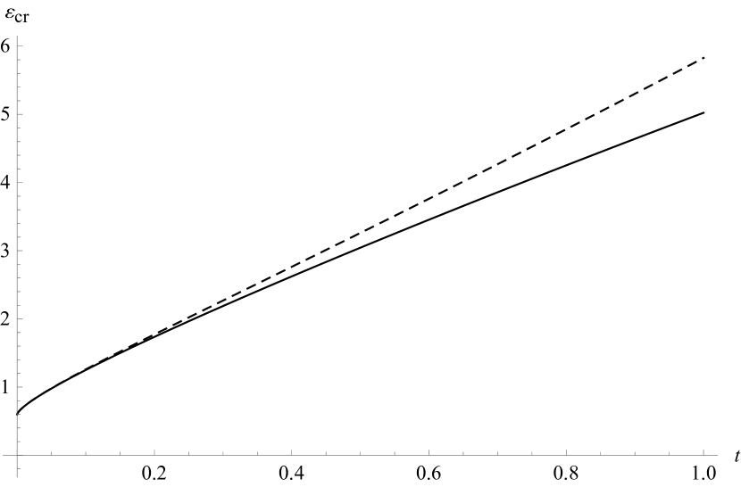
(a) Asymptotics for small time.

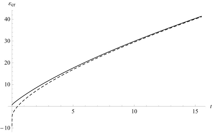
(b) Asymptotics for large time.

Figure 3: Comparison of creep compliance (solid line) and its asymptotic expansions (dashed line).

Figures 4a and 4b display the relaxation modulus, calculated according to (73) in Case 1 and 2, respectively. Model parameters used to produce plots from Figure 4a are the same as for the previous plots guaranteeing that the function $\Psi$ (38) has no zeros in the complex plane (thus corresponding to Case 1) and moreover that the relaxation modulus is a completely monotonic function. Curve from Figure 4b is produced for the model parameters: $\alpha=0.55,$ $\beta=0.8192,$ $a_{1}=1,$ $a_{2}=1.5,$ $a_{3}=1.15,$ $b_{1}=0.2,$ and $b_{2}=0.25,$ guaranteeing that the function $\Psi$ has one negative real zero.

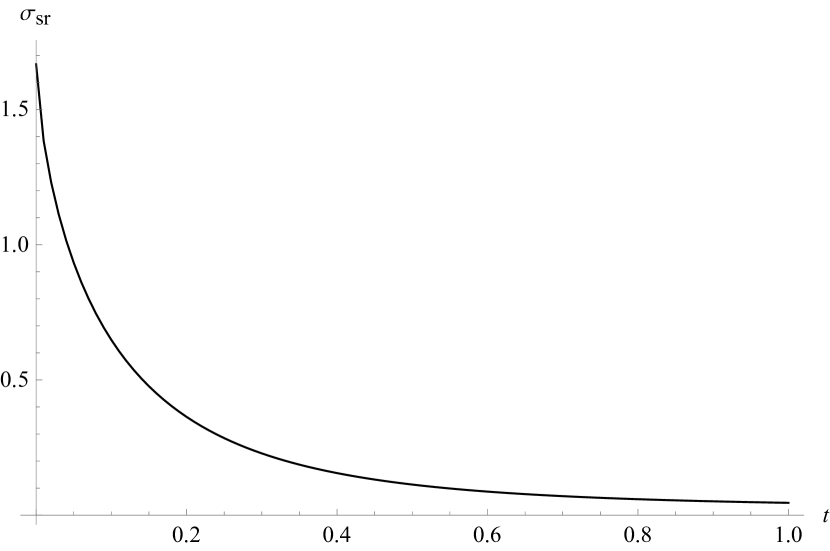
(a) Case 1: completely monotonic function.

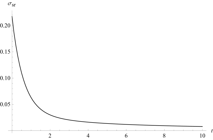
(b) Case 2.

Figure 4: Relaxation modulus in Cases 1 and 2.

Figure 5 displays the relaxation modulus, calculated for model parameters: $\alpha=0.4,$ $\beta=0.95,$ $a_{1}=1.25,$ $a_{2}=1.5,$ $a_{3}=1.15,$ $b_{1}=0.2,$ and $b_{2}=0.25$ according to (73) in Case 3, i.e., in the case when function $\Psi$ (38) has a pair of complex conjugated having negative real part. One notices the non-monotonic behavior of the relaxation modulus.

Figures 6a and 6b display the comparison of relaxation modulus calculated according to (73) in Case 3, presented by the solid line, and its asymptotic expansions near initial time-instant (134) and for large time (136), presented by the dashed line, for the previously mentioned model parameters. Regardless of the non-monotonic behavior of relaxation modulus, the agreement between curves is good.

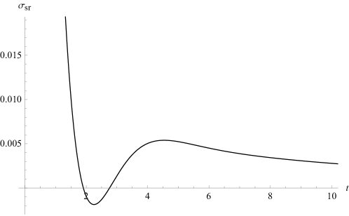
Figure 5: Relaxation modulus in Case 3: oscillatory function having decreasing amplitude.

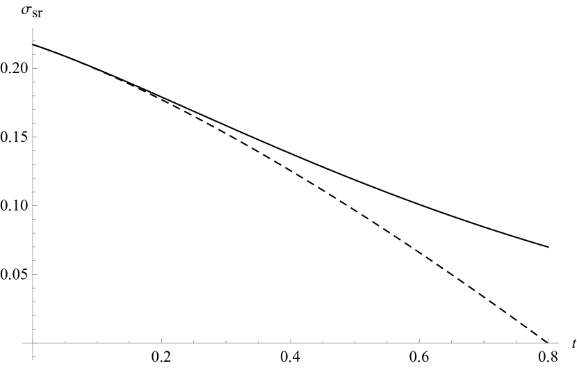
(a) Asymptotics for small time.

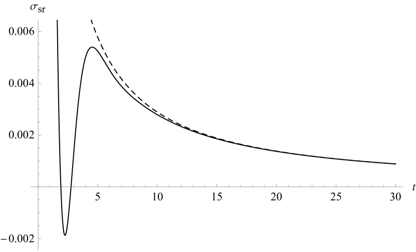
(b) Asymptotics for large time.

Figure 6: Comparison of relaxation modulus (solid line) and its asymptotic expansions (dashed line).

Table 1: Summary of the asymptotic analysis.

	Asymptotics as $t\rightarrow 0$.		Asymptotics as $t\rightarrow\infty$.
Model	creep compliance	relaxation modulus	creep compliance	relaxation modulus
I	$\sim t^{\mu-\gamma+\varkappa}$	$\sim t^{-\left(\mu-\gamma\right)-\varkappa}$	$\sim t^{\mu}$	$\sim t^{-\mu}$
II	$\sim t^{\mu-\alpha}$	$\sim t^{-\left(\mu-\alpha\right)}$
III	$\sim t^{\mu-\beta}$	$\sim t^{-\left(\mu-\beta\right)}$
IV	$\sim t^{\mu-\alpha}$	$\sim t^{-\left(\mu-\alpha\right)}$
V	$\sim t^{\mu-\beta}$	$\sim t^{-\left(\mu-\beta\right)}$
VI	incr. $\sim t^{\alpha}$ from $\frac{a_{3}}{b_{2}}$	decr. $\sim t^{\alpha}$ from $\frac{b_{2}}{a_{3}}$	$\sim t^{\beta}$	$\sim t^{-\beta}$
VII	incr. $\sim t^{\beta}$ from $\frac{a_{3}}{b_{2}}$	decr. $\sim t^{\beta}$ from $\frac{b_{2}}{a_{3}}$
VIII	incr. $\sim t^{\alpha}$ from $\frac{\bar{a}_{2}}{b_{2}}$	decr. $\sim t^{\alpha}$ from $\frac{b_{2}}{\bar{a}_{2}}$	$\sim t^{\alpha}$	$\sim t^{-\alpha}$

6 Conclusion

Thermodynamically consistent classical and fractional Burgers models I - VIII are examined in creep and stress relaxation tests. Using the Laplace transform method, explicit forms of creep compliance in representation via Mittag-Leffler function and in integral representation, as well as the integral representation of relaxation modulus are obtained taking into account the material behavior at initial time-instant, since Models I - V have zero glass compliance (infinite glass modulus), while classical model and Models VI - VIII, have non-zero glass compliance (glass modulus). For all Burgers models equilibrium compliance is infinite implying the zero equilibrium modulus.

By requiring kernels’ non-negativity, the integral forms of the creep compliance and relaxation modulus proved useful in showing that the thermodynamical requirements allow wider range of model parameters than the range in which the creep compliance is a Bernstein function and the relaxation modulus is a completely monotonic function. For the model parameters outside this restrictive interval the creep compliance and relaxation modulus do not have to be monotonic functions. In addition, the relaxation modulus may even be oscillatory function having decreasing amplitude, which is due to the possible zeros of denominator of the relaxation modulus in complex domain, yielding the damped oscillatory term in the relaxation modulus. The conditions for appearance of zeros is independent of the conditions insuring non-negativity of kernel in the integral representation.

The asymptotic analysis of both creep compliance and relaxation modulus conducted in the case of all thermodynamically consistent fractional Burgers models in the vicinity of initial time-instant and for large time as well is summarized in Table 1.

Appendix A Determination of position and number of zeros of functions $\Psi$ and $\Phi$

A.1 Case of function $\Psi$

Introducing the substitution $s=\rho\mathrm{e}^{\mathrm{i}\varphi}$ into function $\Psi,$ given by (38), and by separating real and imaginary parts in $\Psi$ one obtains

$$\mathop{\mathrm{R}e}\Psi\left(\rho,\varphi\right) = 1+a_{1}\rho^{\alpha}\cos\left(\alpha\varphi\right)+a_{2}\rho^{\beta}\cos\left(\beta\varphi\right)+a_{3}\rho^{\gamma}\cos\left(\gamma\varphi\right),$$ (143)

$$\mathop{\mathrm{I}m}\Psi\left(\rho,\varphi\right) = a_{1}\rho^{\alpha}\sin\left(\alpha\varphi\right)+a_{2}\rho^{\beta}\sin\left(\beta\varphi\right)+a_{3}\rho^{\gamma}\sin\left(\gamma\varphi\right),$$ (144)

where $0<\alpha\leq\beta<1,$ $\gamma\in\left(0,2\right),$ and $a_{1},a_{2},a_{3}>0.$ Note that if $s_{0}=\rho_{0}\mathrm{e}^{\mathrm{i}\varphi_{0}},$ $\varphi_{0}\in\left(0,\pi\right),$ is zero of function $\Psi,$ then its complex conjugate, $\bar{s}_{0}=\rho_{0}\mathrm{e}^{-\mathrm{i}\varphi_{0}},$ is also a zero of $\Psi,$ since $\mathop{\mathrm{I}m}\Psi\left(\rho,-\varphi\right)=-\mathop{\mathrm{I}m}\Psi\left(\rho,\varphi\right).$ Therefore, it is sufficient to consider the upper complex half-plane only.

Considering the imaginary part of $\Psi,$ (144), one concludes that function $\Psi$ does not have zeroes in the right complex half-plane. Namely, function $\Psi$ cannot have positive real zeroes, since for $\varphi=0,$ although $\mathop{\mathrm{I}m}\Psi=0$, it holds that $\mathop{\mathrm{R}e}\Psi>0$. Also, since $\alpha,\beta\in\left(0,1\right)$ and $\gamma\in\left(0,2\right),$ for $\varphi\in\left(0,\frac{\pi}{2}\right]$ all sine functions in (144) are positive, implying that $\mathop{\mathrm{I}m}\Psi>0$. Moreover, in the case when $\gamma\in\left(0,1\right),$ function $\Psi$ does not have zeroes in the whole complex plane, since for $\varphi\in\left(0,\pi\right]$ all sine functions in (144) are positive implying that $\mathop{\mathrm{I}m}\Psi>0.$ Therefore, zeros of function $\Psi$ may exist only if $\gamma\in\left(1,2\right),$ and, if zeros exist, they are complex conjugated and located in the left complex half-plane.

In the case when $\gamma\in\left(1,2\right)$, the zeroes of function $\Psi$ will be sought using the argument principle and contour $\Gamma=\Gamma_{1}\cup\Gamma_{2}\cup\Gamma_{3}\cup\Gamma_{4}$ placed in the upper left complex quarter-plane, shown in Figure 7.

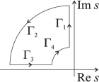
Figure 7: Contour $\Gamma=\Gamma_{1}\cup\Gamma_{2}\cup\Gamma_{3}\cup\Gamma_{4}$.

Parametrizing the contour $\Gamma_{1}$ by $s=\rho\mathrm{e}^{\mathrm{i}\frac{\pi}{2}},$ $\rho\in\left(r,R\right),$ with $r\rightarrow 0$ and $R\rightarrow\infty,$ the real and imaginary parts of $\Psi,$ (143) and (144), become

$$\mathop{\mathrm{R}e}\Psi\left(\rho\right) = 1+a_{1}\rho^{\alpha}\cos\frac{\alpha\pi}{2}+a_{2}\rho^{\beta}\cos\frac{\beta\pi}{2}+a_{3}\rho^{\gamma}\cos\frac{\gamma\pi}{2},$$

$$\mathop{\mathrm{I}m}\Psi\left(\rho\right) = a_{1}\rho^{\alpha}\sin\frac{\alpha\pi}{2}+a_{2}\rho^{\beta}\sin\frac{\beta\pi}{2}+a_{3}\rho^{\gamma}\sin\frac{\gamma\pi}{2}>0,$$

which in the limiting cases yield

$$\mathop{\mathrm{R}e}\Psi\left(\rho\right)\sim 1,\;\;\mathop{\mathrm{I}m}\Psi\left(\rho\right)\sim a_{1}\rho^{\alpha}\sin\frac{\alpha\pi}{2}\rightarrow 0^{+},\;\;\text{as}\;\;\rho=r\rightarrow 0,$$

$$\mathop{\mathrm{R}e}\Psi\left(\rho\right)\sim a_{3}\rho^{\gamma}\cos\frac{\gamma\pi}{2}\rightarrow-\infty,\;\;\mathop{\mathrm{I}m}\Psi\left(\rho\right)\sim a_{3}\rho^{\gamma}\sin\frac{\gamma\pi}{2}\rightarrow\infty,\;\;\text{as}\;\;\rho=R\rightarrow\infty.$$

The real and imaginary parts of $\Psi,$ (143) and (144), along the contour $\Gamma_{2}$, parametrized by $s=R\mathrm{e}^{\mathrm{i}\varphi},$ $\varphi\in\left[\frac{\pi}{2},\pi\right],$ with $R\rightarrow\infty,$ take the form

$$\mathop{\mathrm{R}e}\Psi\left(\varphi\right)\sim a_{3}R^{\gamma}\cos(\gamma\varphi),\;\;\mathop{\mathrm{I}m}\Psi\left(\varphi\right)\sim a_{3}R^{\gamma}\sin(\gamma\varphi),\;\;\text{as}\;\;R\rightarrow\infty.$$ (145)

Note, when $\gamma\in\left(1,\frac{3}{2}\right)$ it holds that $\mathop{\mathrm{R}e}\Psi<0,$ since $\cos(\gamma\varphi)<0.$ If $\varphi=\frac{\pi}{2},$ then (145) becomes

$$\mathop{\mathrm{R}e}\Psi\left(\frac{\pi}{2}\right)\rightarrow-\infty,\;\;\mathop{\mathrm{I}m}\Psi\left(\frac{\pi}{2}\right)\rightarrow\infty,\;\;\text{as}\;\;R\rightarrow\infty,$$

while if $\varphi=\pi,$ then, as $R\rightarrow\infty,$ (145) becomes either

$$\mathop{\mathrm{R}e}\Psi\left(\pi\right)\rightarrow-\infty,\;\;\mathop{\mathrm{I}m}\Psi\left(\pi\right)\rightarrow-\infty,\;\;\text{for}\;\;\gamma\in\left(1,\frac{3}{2}\right),\;\;\text{or}$$

$$\mathop{\mathrm{R}e}\Psi\left(\pi\right)\rightarrow\infty,\;\;\mathop{\mathrm{I}m}\Psi\left(\pi\right)\rightarrow-\infty,\;\;\text{for}\;\;\gamma\in\left[\frac{3}{2},2\right).$$

Using the parametrization $s=\rho\mathrm{e}^{\mathrm{i}\pi},$ $\rho\in\left(r,R\right),$ with $r\rightarrow 0$ and $R\rightarrow\infty,$ of contour $\Gamma_{3},$ the real and imaginary parts of $\Psi,$ (143) and (144), become

$$\mathop{\mathrm{R}e}\Psi\left(\rho\right) = 1+a_{1}\rho^{\alpha}\cos\left(\alpha\pi\right)+a_{2}\rho^{\beta}\cos\left(\beta\pi\right)+a_{3}\rho^{\gamma}\cos\left(\gamma\pi\right),$$ (146)

$$\mathop{\mathrm{I}m}\Psi\left(\rho\right) = a_{1}\rho^{\alpha}\sin\left(\alpha\pi\right)+a_{2}\rho^{\beta}\sin\left(\beta\pi\right)+a_{3}\rho^{\gamma}\sin\left(\gamma\pi\right),$$ (147)

which, as $\rho=r\rightarrow 0,$ yield

$$\mathop{\mathrm{R}e}\Psi\left(\rho\right)\sim 1,\;\;\mathop{\mathrm{I}m}\Psi\left(\rho\right)\sim a_{1}\rho^{\alpha}\sin\left(\alpha\pi\right)\rightarrow 0^{+},$$

and, as $\rho=R\rightarrow\infty,$ either

$$\mathop{\mathrm{R}e}\Psi\left(\rho\right)\sim a_{3}\rho^{\gamma}\cos\left(\gamma\pi\right)\rightarrow-\infty,\;\;\mathop{\mathrm{I}m}\Psi\left(\rho\right)\sim a_{3}\rho^{\gamma}\sin\left(\gamma\pi\right)\rightarrow\infty,\;\;\text{for}\;\;\gamma\in\left(1,\frac{3}{2}\right),\;\;\text{or}$$

$$\mathop{\mathrm{R}e}\Psi\left(\rho\right)\sim a_{3}\rho^{\gamma}\cos\left(\gamma\pi\right)\rightarrow\infty,\;\;\mathop{\mathrm{I}m}\Psi\left(\rho\right)\sim a_{3}\rho^{\gamma}\sin\left(\gamma\pi\right)\rightarrow\infty,\;\;\text{for}\;\;\gamma\in\left[\frac{3}{2},2\right),$$

Since $\alpha,\beta\in\left(0,1\right)$ and $\gamma\in\left(1,2\right),$ the first two terms in (147) are positive, while the third term is negative, so that there exists at least one $\rho^{\ast}\neq 0$ such that

$$\mathop{\mathrm{I}m}\Psi\left(\rho^{\ast}\right)=a_{3}\left(\rho^{\ast}\right)^{\alpha}\left|\sin\left(\gamma\pi\right)\right|\left(\frac{a_{1}\sin\left(\alpha\pi\right)}{a_{3}\left|\sin\left(\gamma\pi\right)\right|}+\frac{a_{2}\sin\left(\beta\pi\right)}{a_{3}\left|\sin\left(\gamma\pi\right)\right|}\left(\rho^{\ast}\right)^{\beta-\alpha}-\left(\rho^{\ast}\right)^{\gamma-\alpha}\right)=0.$$

The equation

$$\frac{a_{1}\sin\left(\alpha\pi\right)}{a_{3}\left|\sin\left(\gamma\pi\right)\right|}+\frac{a_{2}\sin\left(\beta\pi\right)}{a_{3}\left|\sin\left(\gamma\pi\right)\right|}\left(\rho^{\ast}\right)^{\beta-\alpha}=\left(\rho^{\ast}\right)^{\gamma-\alpha}$$ (148)

has a single solution $\rho^{\ast}.$ Namely, since $0<\alpha\leq\beta<1$ and $\gamma\in\left(1,2\right),$ the function $\left(\rho^{\ast}\right)^{\beta-\alpha}$ is concave, due to $\beta-\alpha\in\left(0,1\right)$ (or even constant if $\beta=\alpha$), and $\left(\rho^{\ast}\right)^{\gamma-\alpha}$ is either convex, if $\gamma-\alpha\in\left(1,2\right)$, or concave, if $\gamma-\alpha\in\left(0,1\right)$ (or even linear if $\gamma-\alpha=1$), but always increases faster than $\left(\rho^{\ast}\right)^{\beta-\alpha}.$ Depending on the value of $\rho^{\ast},$ the real part of $\Psi,$ (146), can be either negative, zero, or positive, which will determine the change of argument of function $\Psi$ along the contour $\Gamma.$

Along the contour $\Gamma_{4},$ parametrized by $s=r\mathrm{e}^{\mathrm{i}\varphi},$ $\varphi\in\left[\frac{\pi}{2},\pi\right],$ with $r\rightarrow 0,$ the real and imaginary parts of $\Psi,$ (143) and (144), take the form

$$\mathop{\mathrm{R}e}\Psi\left(\varphi\right)\sim 1,\;\;\mathop{\mathrm{I}m}\Psi\left(\varphi\right)\sim a_{1}r^{\gamma}\sin(\alpha\varphi)>0,\;\;\text{as}\;\;r\rightarrow 0,$$

so that $\mathop{\mathrm{I}m}\Psi\left(\varphi\right)\rightarrow 0^{+},$ for $\varphi\in\left[\frac{\pi}{2},\pi\right],$ as $r\rightarrow 0.$

By the argument principle, function $\Psi$ has no zeros (has one complex zero) in the upper left complex quarter-plane if $\mathop{\mathrm{R}e}\Psi\left(\rho^{\ast}\right)<0$ ($\mathop{\mathrm{R}e}\Psi\left(\rho^{\ast}\right)>0$) in (146), since the change of argument of function $\Psi$ is $\Delta\arg\Psi=0$ ($\Delta\arg\Psi=2\pi$) along the contour $\Gamma,$ while if $\mathop{\mathrm{R}e}\Psi\left(\rho^{\ast}\right)=0,$ then function $\Psi$ has a negative real zero $-\rho^{\ast},$ with $\rho^{\ast}$ determined from (148). This holds true for the whole complex plane as well if $\gamma\in\left(1,2\right),$ while if $\gamma\in\left(0,1\right),$ then function $\Psi$ does not have zeros in the complex plane.

A.2 Case of function $\Phi$

Function $\Phi,$ given by (59), being a quadratic function in terms of $s^{\alpha},$ is decomposed as

$$\Phi\left(s\right)=\bar{a}_{2}\left(s^{\alpha}+a_{1}\right)\left(s^{\alpha}+a_{2}\right),\;\;\text{with}\;\;a_{1,2}=\frac{\bar{a}_{1}}{2\bar{a}_{2}}\pm\sqrt{\left(\frac{\bar{a}_{1}}{2\bar{a}_{2}}\right)^{2}-\frac{1}{\bar{a}_{2}}}>0,$$

for $\left(\frac{\bar{a}_{1}}{2\bar{a}_{2}}\right)^{2}\geq\frac{1}{\bar{a}_{2}},$ implying that function $\Phi$ has no zeros in the principal Riemann branch, i.e., for $\arg s\in\left(-\pi,\pi\right),$ since it is well-known that equation

$$s^{\alpha}+a_{1,2}=0,\;\;s\in\mathbb{C},$$

has no solutions for $\arg s\in\left(-\pi,\pi\right).$

For $\left(\frac{\bar{a}_{1}}{2\bar{a}_{2}}\right)^{2}<\frac{1}{\bar{a}_{2}},$ function $\Phi$ is decomposed as

$$\Phi\left(s\right)=\bar{a}_{2}\left(s^{\alpha}+a-\mathrm{i}b\right)\left(s^{\alpha}+a+\mathrm{i}b\right),\;\;\text{with}\;\;a=\frac{\bar{a}_{1}}{2\bar{a}_{2}}\;\;\text{and}\;\;b=\sqrt{\frac{1}{\bar{a}_{2}}-\left(\frac{\bar{a}_{1}}{2\bar{a}_{2}}\right)^{2}}.$$

Define a function $\phi$ by

$$\phi\left(s\right)=s^{\alpha}+a-\mathrm{i}b,\;\;s\in\mathbb{C},$$ (149)

where $\alpha\in\left(0,1\right),$ The real and imaginary parts of function $\phi$ are obtained as

$$\mathop{\mathrm{R}e}\phi\left(\rho,\varphi\right) = \rho^{\alpha}\cos\left(\alpha\varphi\right)+a,$$ (150)

$$\mathop{\mathrm{I}m}\phi\left(\rho,\varphi\right) = \rho^{\alpha}\sin\left(\alpha\varphi\right)-b,$$ (151)

using $s=\rho\mathrm{e}^{\mathrm{i}\varphi}$ in (149). If function $\phi$ has zero $s_{0}=\rho_{0}\mathrm{e}^{\mathrm{i}\varphi_{0}}$ in the upper complex half-plane (since $\sin\left(\alpha\varphi\right)>0$ for $\varphi\in\left(0,\pi\right)$), then the complex conjugated zero $\bar{s}_{0}=\rho_{0}\mathrm{e}^{-\mathrm{i}\varphi_{0}}$ is obtained as a solution of equation $s^{\alpha}+a+\mathrm{i}b=0.$ Thus, $s_{0}$ and $\bar{s}_{0}$ are complex conjugated zeros of function $\Phi$ as well. Function $\phi$ does not have zeroes in the upper right complex quarter-plane, since for $\varphi\in\left[0,\frac{\pi}{2}\right]$ its real part (150) is positive.

Therefore, the zeros of $\phi$ will be sought for in the upper left complex quarter-plane within the contour $\Gamma,$ shown in Figure 7, by using the argument principle. Parametrizing the contour $\Gamma=\Gamma_{1}\cup\Gamma_{2}\cup\Gamma_{3}\cup\Gamma_{4}$ as in Section A.1, along $\Gamma_{1},$ by (150) and (151), one obtains

$$\mathop{\mathrm{R}e}\phi\left(\rho\right)=\rho^{\alpha}\cos\frac{\alpha\pi}{2}+a>0,\;\;\mathop{\mathrm{I}m}\phi\left(\rho\right)=\rho^{\alpha}\sin\frac{\alpha\pi}{2}-b,$$

$$\mathop{\mathrm{R}e}\phi\left(\rho\right)\sim a,\;\;\mathop{\mathrm{I}m}\phi\left(\rho\right)\sim-b,\;\;\text{as}\;\;\rho=r\rightarrow 0,$$

$$\mathop{\mathrm{R}e}\phi\left(\rho\right)\rightarrow\infty,\;\;\mathop{\mathrm{I}m}\phi\left(\rho\right)\rightarrow\infty,\;\;\text{as}\;\;\rho=R\rightarrow\infty,$$

as real and imaginary parts of $\phi$, and their limiting cases. Along $\Gamma_{2},$ as $R\rightarrow\infty,$ for arbitrary value of $\varphi$, as well as for $\varphi=\frac{\pi}{2}$ and $\varphi=\pi,$ (150) and (151) take the following forms

$$\mathop{\mathrm{R}e}\phi\left(\varphi\right)\sim R^{\alpha}\cos(\alpha\varphi),\;\;\mathop{\mathrm{I}m}\phi\left(\varphi\right)\sim R^{\alpha}\sin(\alpha\varphi)>0,$$

$$\mathop{\mathrm{R}e}\phi\left(\frac{\pi}{2}\right)\rightarrow\infty,\;\;\mathop{\mathrm{I}m}\phi\left(\frac{\pi}{2}\right)\rightarrow\infty,$$

$$\mathop{\mathrm{R}e}\phi\left(\pi\right)\rightarrow-\infty,\;\;\mathop{\mathrm{I}m}\phi\left(\pi\right)\rightarrow\infty.$$

In the case of contour $\Gamma_{3},$ (150), (151) and their limiting cases are

$$\mathop{\mathrm{R}e}\phi\left(\rho\right)=-\rho^{\alpha}\left|\cos\left(\alpha\pi\right)\right|+a,\;\;\mathop{\mathrm{I}m}\phi\left(\rho\right)=\rho^{\alpha}\sin\left(\alpha\pi\right)-b,$$ (152)

$$\mathop{\mathrm{R}e}\phi\left(\rho\right)\sim a,\;\;\mathop{\mathrm{I}m}\phi\left(\rho\right)\sim-b,\;\;\text{as}\;\;\rho=r\rightarrow 0,$$

$$\mathop{\mathrm{R}e}\phi\left(\rho\right)\rightarrow-\infty,\;\;\mathop{\mathrm{I}m}\phi\left(\rho\right)\rightarrow\infty,\;\;\text{as}\;\;\rho=R\rightarrow\infty.$$

Depending on the value of solution $\rho^{\ast}=\left(\frac{b}{\sin\left(\alpha\pi\right)}\right)^{\frac{1}{\alpha}}$ of equation $\mathop{\mathrm{I}m}\phi\left(\rho^{\ast}\right)=0,$ (152)${}_{2},$ the real part of $\phi,$ (152)₁, can be either negative, zero, or positive, which will determine the change of argument of function $\phi$ along the whole contour $\Gamma.$ Along the contour $\Gamma_{4},$ one has

$$\mathop{\mathrm{R}e}\phi\left(\varphi\right)\sim a,\;\;\mathop{\mathrm{I}m}\phi\left(\varphi\right)\sim-b^{+},\;\;\text{as}\;\;r\rightarrow 0.$$

By the argument principle, function $\phi$ has no zeros (has one complex zero) in the upper left complex quarter-plane and therefore in the whole upper complex half-plane as well, if $\mathop{\mathrm{R}e}\phi\left(\rho^{\ast}\right)=-b\frac{\left|\cos\left(\alpha\pi\right)\right|}{\sin\left(\alpha\pi\right)}+a<0$ ($\mathop{\mathrm{R}e}\phi\left(\rho^{\ast}\right)=-b\frac{\left|\cos\left(\alpha\pi\right)\right|}{\sin\left(\alpha\pi\right)}+a>0$) in (152), since the change of argument of function $\phi$ is $\Delta\arg\phi=0$ ($\Delta\arg\phi=2\pi$) along the contour $\Gamma$. If $\mathop{\mathrm{R}e}\phi\left(\rho^{\ast}\right)=0,$ then function $\phi$ has a negative real zero $-\rho^{\ast}.$

Appendix B Calculation of creep compliance and relaxation modulus

The creep compliance and relaxation modulus corresponding to Models I - V, respectively to Models VI and VII, will be obtained in the integral forms (49) and (65), respectively as (51) and (73), by inverting the creep compliance and relaxation modulus in complex domain, given by (35) and (56), respectively by (36) and (57), using the definition of inverse Laplace transform

$$f\left(t\right)=\mathcal{L}^{-1}\left[\tilde{f}\left(s\right)\right]\left(t\right)=\frac{1}{2\pi\mathrm{i}}\int_{p_{0}-\mathrm{i}\infty}^{p_{0}+\mathrm{i}\infty}\tilde{f}\left(s\right)\mathrm{e}^{st}\mathrm{d}s.$$ (153)

In the case of creep compliance in complex domain, as well as for the relaxation modulus in complex domain when function $\Psi,$ given by (38), has either no zeros in complex plane, or has one negative real zero, the Laplace transform inversion will be performed by using the Cauchy integral theorem $\oint_{\Gamma}f(z)\mathrm{d}z=0.$ In the case of relaxation modulus in complex domain when function $\Psi$ (38) has a pair of complex conjugated zeros, the Cauchy residue theorem $\oint_{\Gamma}f(z)\mathrm{d}z=2\pi\mathrm{i}\sum_{k}\mathop{\mathrm{R}es}\left(f\left(z\right),z_{k}\right)$ will be employed.

In the case of Model VIII, the creep compliance and relaxation modulus, given by (53) and (81), are also calculated by the Laplace transform inversion of the creep compliance and relaxation modulus in complex domain, given by (37) and (58). Being analogous to the case of Models VI and VII the calculation is omitted.

B.1 Calculation of creep compliance

B.1.1 Creep compliance in the case of models having zero glass compliance

The rate of creep is obtained as

$$\dot{\varepsilon}_{cr}\left(t\right)=\mathcal{L}^{-1}\left[s\tilde{\varepsilon}_{cr}\left(s\right)\right]\left(t\right)=\frac{1}{2\pi\mathrm{i}}\lim_{\begin{subarray}{c}R\rightarrow\infty,\\ r\rightarrow 0\end{subarray}}\int_{\Gamma_{0}}s\tilde{\varepsilon}_{cr}\left(s\right)\mathrm{e}^{st}\mathrm{d}s,$$ (154)

using the inverse Laplace transform (153) of the creep compliance in complex domain (35) and zero value of the glass compliance (44). The Cauchy integral theorem

$$\oint_{\Gamma^{\left(\mathrm{I}\right)}}s\tilde{\varepsilon}_{cr}\left(s\right)\mathrm{e}^{st}\mathrm{d}s=0,$$ (155)

where the contour $\Gamma^{\left(\mathrm{I}\right)}=\Gamma_{0}\cup\Gamma_{1}\cup\Gamma_{2}\cup\Gamma_{3}\cup\Gamma_{4}\cup\Gamma_{5}\cup\Gamma_{6}\cup\Gamma_{7}$ is chosen as in Figure 8,

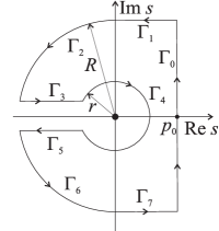
Figure 8: Contour $\Gamma^{\left(\mathrm{I}\right)}.$

yields the rate of creep in the form

$$\dot{\varepsilon}_{cr}\left(t\right) = \frac{1}{2\pi\mathrm{i}}\int_{0}^{\infty}\left(\frac{\Psi\left(\rho\mathrm{e}^{-\mathrm{i}\pi}\right)}{b_{1}+b_{2}\rho^{\eta}\mathrm{e}^{-\mathrm{i}\eta\pi}}\mathrm{e}^{\mathrm{i}\mu\pi}-\frac{\Psi\left(\rho\mathrm{e}^{\mathrm{i}\pi}\right)}{b_{1}+b_{2}\rho^{\eta}\mathrm{e}^{\mathrm{i}\eta\pi}}\mathrm{e}^{-\mathrm{i}\mu\pi}\right)\frac{\mathrm{e}^{-\rho t}}{\rho^{\mu}}\mathrm{d}\rho$$ (156)

$$= \frac{1}{\pi}\int_{0}^{\infty}\frac{K\left(\rho\right)}{\left|b_{1}+b_{2}\rho^{\eta}\mathrm{e}^{\mathrm{i}\eta\pi}\right|^{2}}\frac{\mathrm{e}^{-\rho t}}{\rho^{\mu}}\mathrm{d}\rho,$$ (157)

and thus the creep compliance becomes

$$\varepsilon_{cr}\left(t\right)=\frac{1}{\pi}\int_{0}^{\infty}\frac{K\left(\rho\right)}{\left|b_{1}+b_{2}\rho^{\eta}\mathrm{e}^{\mathrm{i}\eta\pi}\right|^{2}}\frac{1-\mathrm{e}^{-\rho t}}{\rho^{1+\mu}}\mathrm{d}\rho,$$

where,

$$K\left(\rho\right) = b_{1}K_{1}\left(\rho\right)+b_{2}\rho^{\eta}K_{2}\left(\rho\right),\;\;\text{with}$$

$$K_{1}\left(\rho\right) = \sin\left(\mu\pi\right)\mathop{\mathrm{R}e}\Psi\left(\rho\mathrm{e}^{\mathrm{i}\pi}\right)-\cos\left(\mu\pi\right)\mathop{\mathrm{I}m}\Psi\left(\rho\mathrm{e}^{\mathrm{i}\pi}\right)$$

$$= \sin\left(\mu\pi\right)+a_{1}\rho^{\alpha}\sin\left(\left(\mu-\alpha\right)\pi\right)+a_{2}\rho^{\beta}\sin\left(\left(\mu-\beta\right)\pi\right)+a_{3}\rho^{\gamma}\sin\left(\left(\mu-\gamma\right)\pi\right),$$

$$K_{2}\left(\rho\right) = \sin\left(\left(\mu+\eta\right)\pi\right)\mathop{\mathrm{R}e}\Psi\left(\rho\mathrm{e}^{\mathrm{i}\pi}\right)-\cos\left(\left(\mu+\eta\right)\pi\right)\mathop{\mathrm{I}m}\Psi\left(\rho\mathrm{e}^{\mathrm{i}\pi}\right)$$

$$= \sin\left(\left(\mu+\eta\right)\pi\right)+a_{1}\rho^{\alpha}\sin\left(\left(\mu+\eta-\alpha\right)\pi\right)+a_{2}\rho^{\beta}\sin\left(\left(\mu+\eta-\beta\right)\pi\right)+a_{3}\rho^{\gamma}\sin\left(\left(\mu+\eta-\gamma\right)\pi\right),$$

since $\Psi\left(\bar{s}\right)=-\bar{\Psi}\left(s\right).$

The integrals along contours $\Gamma_{3}$ (parametrized by $s=\rho\mathrm{e}^{\mathrm{i}\pi},$ $\rho\in\left(r,R\right)$) and $\Gamma_{5}$ (parametrized by $s=\rho\mathrm{e}^{-\mathrm{i}\pi},$ $\rho\in\left(r,R\right)$) read

$$\lim_{\begin{subarray}{c}R\rightarrow\infty,\\ r\rightarrow 0\end{subarray}}\int_{\Gamma_{3}}s\tilde{\varepsilon}_{cr}\left(s\right)\mathrm{e}^{st}\mathrm{d}s = \int_{\infty}^{0}\frac{1}{\rho^{\mu}\mathrm{e}^{\mathrm{i}\mu\pi}}\frac{\Psi\left(\rho\mathrm{e}^{\mathrm{i}\pi}\right)}{b_{1}+b_{2}\rho^{\eta}\mathrm{e}^{\mathrm{i}\eta\pi}}\mathrm{e}^{-\rho t}\mathrm{e}^{\mathrm{i}\pi}\mathrm{d}\rho=\int_{0}^{\infty}\frac{\Psi\left(\rho\mathrm{e}^{\mathrm{i}\pi}\right)}{b_{1}+b_{2}\rho^{\eta}\mathrm{e}^{\mathrm{i}\eta\pi}}\mathrm{e}^{-\mathrm{i}\mu\pi}\frac{\mathrm{e}^{-\rho t}}{\rho^{\mu}}\mathrm{d}\rho,$$

$$\lim_{\begin{subarray}{c}R\rightarrow\infty,\\ r\rightarrow 0\end{subarray}}\int_{\Gamma_{5}}s\tilde{\varepsilon}_{cr}\left(s\right)\mathrm{e}^{st}\mathrm{d}s = \int_{0}^{\infty}\frac{1}{\rho^{\mu}\mathrm{e}^{-\mathrm{i}\mu\pi}}\frac{\Psi\left(\rho\mathrm{e}^{-\mathrm{i}\pi}\right)}{b_{1}+b_{2}\rho^{\eta}\mathrm{e}^{-\mathrm{i}\eta\pi}}\mathrm{e}^{-\rho t}\mathrm{e}^{-\mathrm{i}\pi}\mathrm{d}\rho=-\int_{0}^{\infty}\frac{\Psi\left(\rho\mathrm{e}^{-\mathrm{i}\pi}\right)}{b_{1}+b_{2}\rho^{\eta}\mathrm{e}^{-\mathrm{i}\eta\pi}}\mathrm{e}^{\mathrm{i}\mu\pi}\frac{\mathrm{e}^{-\rho t}}{\rho^{\mu}}\mathrm{d}\rho,$$

yielding the rate of creep (156) according to the Cauchy integral theorem (155), since the inverse Laplace transform of the rate of creep in complex domain is (154) and integrals along $\Gamma_{1},$ $\Gamma_{2},$ $\Gamma_{4},$ $\Gamma_{6},$ $\Gamma_{7}$ tend to zero as $R\rightarrow\infty$ and $r\rightarrow 0.$

The contour $\Gamma_{1}$ is parametrized by $s=p+\mathrm{i}R,$ $p\in\left(0,p_{0}\right),$ with $R\rightarrow\infty,$ so that the integral

$$I_{\Gamma_{1}}=\int_{\Gamma_{1}}s\tilde{\varepsilon}_{cr}\left(s\right)\mathrm{e}^{st}\mathrm{d}s=\int_{0}^{p_{0}}\frac{1}{(p+\mathrm{i}R)^{\mu}}\frac{\Psi\left(p+\mathrm{i}R\right)}{b_{1}+b_{2}(p+\mathrm{i}R)^{\eta}}\mathrm{e}^{\left(p+\mathrm{i}R\right)t}\mathrm{d}p$$

is estimated as

$$\left|I_{\Gamma_{1}}\right|\leq\int_{0}^{p_{0}}\frac{1}{\left|p+\mathrm{i}R\right|^{\mu}}\frac{\left|\Psi\left(p+\mathrm{i}R\right)\right|}{\left|b_{1}+b_{2}(p+\mathrm{i}R)^{\eta}\right|}\mathrm{e}^{pt}\mathrm{d}p.$$ (158)

Assuming $s=\rho\mathrm{e}^{\mathrm{i}\varphi},$ since $R\rightarrow\infty,$ one obtains $\rho=\sqrt{p^{2}+R^{2}}\sim R$ and $\varphi=\arctan\frac{R}{p}\sim\frac{\pi}{2},$ so that (158) becomes

$$\lim_{R\rightarrow\infty}\left|I_{\Gamma_{1}}\right|\leq\lim_{R\rightarrow\infty}\int_{0}^{p_{0}}\frac{1}{R^{\mu}}\frac{\left|\Psi\left(R\mathrm{e}^{\mathrm{i}\frac{\pi}{2}}\right)\right|}{\left|b_{1}+b_{2}R^{\eta}\mathrm{e}^{\mathrm{i}\frac{\eta\pi}{2}}\right|}\mathrm{e}^{pt}\mathrm{d}p\leq\frac{a_{3}}{b_{2}}\lim_{R\rightarrow\infty}\int_{0}^{p_{0}}\frac{1}{R^{\mu+\eta-\gamma}}\mathrm{e}^{pt}\mathrm{d}p=0,$$

since, by (38) one has

$$\left|\Psi\left(R\mathrm{e}^{\mathrm{i}\frac{\pi}{2}}\right)\right|\sim a_{3}R^{\gamma},\;\;\text{as}\;\;R\rightarrow\infty,$$ (159)

as well as

μ−α,for Models II and IV,μ−β,for Models III and V,∈(0,1),\mu+\eta-\gamma=\left\{\begin{tabular}[]{ll}$\mu,$ or $\mu-\left(\gamma-\beta\right),$ or $\mu-\left(\gamma-\alpha\right),$&for Model I,\\ $\mu-\alpha,$&for Models II and IV,\\ $\mu-\beta,$&for Models III and V,\end{tabular}\right.\in\left(0,1\right),

μ, or -μ(-γβ), or -μ(-γα), for Model I, (160)

due to $\eta=\kappa\in\left\{\alpha,\beta,\gamma\right\}$, with thermodynamical restriction (5) for Model I, and due to $\left(\eta,\gamma\right)\in\{\left(\alpha,2\alpha\right),$ $\left(\alpha,\alpha+\beta\right),$ $\left(\beta,\alpha+\beta\right),$ $\left(\beta,2\beta\right)\},$ with thermodynamical restrictions (7), (9), (11), and (13) for Models II - V. Analogously, it can be proved that $\lim_{R\rightarrow\infty}\left|I_{\Gamma_{7}}\right|=0.$

The integral along contour $\Gamma_{2},$ parametrized by $s=R\mathrm{e}^{\mathrm{i}\varphi},$ $\varphi\in\left(\frac{\pi}{2},\pi\right),$ with $R\rightarrow\infty,$ is

$$I_{\Gamma_{2}}=\int_{\Gamma_{2}}s\tilde{\varepsilon}_{cr}\left(s\right)\mathrm{e}^{st}\mathrm{d}s=\int_{\frac{\pi}{2}}^{\pi}\frac{1}{R^{\mu}\mathrm{e}^{\mathrm{i}\mu\varphi}}\frac{\Psi\left(R\mathrm{e}^{\mathrm{i}\varphi}\right)}{b_{1}+b_{2}R^{\eta}\mathrm{e}^{\mathrm{i}\eta\varphi}}\mathrm{e}^{Rt\mathrm{e}^{\mathrm{i}\varphi}}\mathrm{i}R\mathrm{e}^{\mathrm{i}\varphi}\mathrm{d}\varphi,$$

yielding the estimate

$$\left|I_{\Gamma_{2}}\right|\leq\int_{\frac{\pi}{2}}^{\pi}R^{1-\mu}\frac{\left|\Psi\left(R\mathrm{e}^{\mathrm{i}\varphi}\right)\right|}{\left|b_{1}+b_{2}R^{\eta}\mathrm{e}^{\mathrm{i}\eta\varphi}\right|}\mathrm{e}^{Rt\cos\varphi}\mathrm{d}\varphi.$$ (161)

Similarly as in (159), one has $\left|\Psi\left(R\mathrm{e}^{\mathrm{i}\varphi}\right)\right|\sim a_{3}R^{\gamma},$ as $R\rightarrow\infty,$ which, along with $\cos\varphi<0$ for $\varphi\in\left(\frac{\pi}{2},\pi\right),$ implies that (161) in the limit when $R\rightarrow\infty$ becomes

$$\lim_{R\rightarrow\infty}\left|I_{\Gamma_{2}}\right|\leq\frac{a_{3}}{b_{2}}\lim_{R\rightarrow\infty}\int_{\frac{\pi}{2}}^{\pi}R^{1-\left(\mu+\eta-\gamma\right)}\mathrm{e}^{Rt\cos\varphi}\mathrm{d}\varphi=0,$$

although, by (160), $1-\left(\mu+\eta-\gamma\right)>0.$ By the similar arguments, $\lim_{R\rightarrow\infty}\left|I_{\Gamma_{6}}\right|=0,$ as well.

Parametrization of the contour $\Gamma_{4}$ is $s=r\mathrm{e}^{\mathrm{i}\varphi},$ $\varphi\in\left(-\pi,\pi\right),$ with $r\rightarrow 0,$ so that

$$I_{\Gamma_{4}}=\int_{\Gamma_{4}}s\tilde{\varepsilon}_{cr}\left(s\right)\mathrm{e}^{st}\mathrm{d}s=\int_{-\pi}^{\pi}\frac{1}{r^{\mu}\mathrm{e}^{\mathrm{i}\mu\varphi}}\frac{\Psi\left(r\mathrm{e}^{\mathrm{i}\varphi}\right)}{b_{1}+b_{2}r^{\eta}\mathrm{e}^{\mathrm{i}\eta\varphi}}\mathrm{e}^{rt\mathrm{e}^{\mathrm{i}\varphi}}\mathrm{i}r\mathrm{e}^{\mathrm{i}\varphi}\mathrm{d}\varphi$$

can be estimated by

$$\lim_{r\rightarrow 0}\left|I_{\Gamma_{4}}\right|\leq\lim_{r\rightarrow 0}\int_{-\pi}^{\pi}r^{1-\mu}\frac{\left|\Psi\left(r\mathrm{e}^{\mathrm{i}\varphi}\right)\right|}{\left|b_{1}+b_{2}r^{\eta}\mathrm{e}^{\mathrm{i}\eta\varphi}\right|}\mathrm{e}^{rt\cos\varphi}\mathrm{d}\varphi\leq\frac{2\pi}{b_{1}}\lim_{r\rightarrow 0}r^{1-\mu}=0,$$

since $\left|\Psi\left(r\mathrm{e}^{\mathrm{i}\varphi}\right)\right|\sim 1$ as $r\rightarrow 0.$

B.1.2 Creep compliance in the case of models having non-zero glass compliance

Inverting the Laplace transform in the creep compliance in complex domain (36), the creep compliance is obtained in the form

$$\varepsilon_{cr}\left(t\right)=\frac{a_{3}}{b_{2}}+\frac{a_{3}}{b_{2}}\int_{0}^{t}f_{cr}\left(\tau\right)\mathrm{d}\tau,$$

where $\varepsilon_{cr}^{\left(g\right)}=\frac{a_{3}}{b_{2}}$ is the glass compliance (44) and function $f_{cr}$ is defined by its Laplace transform as

$$\tilde{f}_{cr}\left(s\right)=\mathcal{L}\left[f_{cr}\left(t\right)\right]\left(s\right)=\frac{1}{s^{\beta}}\frac{\psi\left(s\right)}{\frac{b_{1}}{b_{2}}+s^{\eta}},$$

with function $\psi$ defined by (39). Function $f_{cr},$ having the form

$$f_{cr}\left(t\right) = \frac{1}{2\pi\mathrm{i}}\int_{0}^{\infty}\left(\frac{\psi\left(\rho\mathrm{e}^{-\mathrm{i}\pi}\right)}{\frac{b_{1}}{b_{2}}+\rho^{\eta}\mathrm{e}^{-\mathrm{i}\eta\pi}}\mathrm{e}^{\mathrm{i}\beta\pi}-\frac{\psi\left(\rho\mathrm{e}^{\mathrm{i}\pi}\right)}{\frac{b_{1}}{b_{2}}+\rho^{\eta}\mathrm{e}^{\mathrm{i}\eta\pi}}\mathrm{e}^{-\mathrm{i}\beta\pi}\right)\frac{\mathrm{e}^{-\rho t}}{\rho^{\beta}}\mathrm{d}\rho$$

$$= \frac{1}{\pi}\int_{0}^{\infty}\frac{Q\left(\rho\right)}{\left|\frac{b_{1}}{b_{2}}+\rho^{\eta}\mathrm{e}^{\mathrm{i}\eta\pi}\right|^{2}}\frac{\mathrm{e}^{-\rho t}}{\rho^{\beta}}\mathrm{d}\rho,$$

where, due to $\psi\left(\bar{s}\right)=-\bar{\psi}\left(s\right),$

$$Q\left(\rho\right) = \frac{b_{1}}{b_{2}}Q_{1}\left(\rho\right)+\rho^{\eta}Q_{2}\left(\rho\right),\;\;\text{with}$$

$$Q_{1}\left(\rho\right) = \sin\left(\beta\pi\right)\mathop{\mathrm{R}e}\psi\left(\rho\mathrm{e}^{\mathrm{i}\pi}\right)-\cos\left(\beta\pi\right)\mathop{\mathrm{I}m}\psi\left(\rho\mathrm{e}^{\mathrm{i}\pi}\right)$$

$$= \frac{1}{a_{3}}\sin\left(\beta\pi\right)+\frac{a_{1}}{a_{3}}\rho^{\alpha}\sin\left(\left(\beta-\alpha\right)\pi\right),$$

$$Q_{2}\left(\rho\right) = \sin\left(\left(\beta+\eta\right)\pi\right)\mathop{\mathrm{R}e}\psi\left(\rho\mathrm{e}^{\mathrm{i}\pi}\right)-\cos\left(\left(\beta+\eta\right)\pi\right)\mathop{\mathrm{I}m}\psi\left(\rho\mathrm{e}^{\mathrm{i}\pi}\right)$$

$$= \frac{1}{a_{3}}\sin\left(\left(\beta+\eta\right)\pi\right)+\frac{a_{1}}{a_{3}}\rho^{\alpha}\sin\left(\left(\beta+\eta-\alpha\right)\pi\right)+\left(\frac{a_{2}}{a_{3}}-\frac{b_{1}}{b_{2}}\right)\rho^{\beta}\sin\left(\eta\pi\right),$$

is calculated by the inverse Laplace transform

$$f_{cr}\left(t\right)=\frac{1}{2\pi\mathrm{i}}\lim_{\begin{subarray}{c}R\rightarrow\infty,\\ r\rightarrow 0\end{subarray}}\int_{\Gamma_{0}}\tilde{f}_{cr}\left(s\right)\mathrm{e}^{st}\mathrm{d}s,$$

see (153), using the Cauchy integral theorem

$$\oint_{\Gamma^{\left(\mathrm{I}\right)}}\tilde{f}_{cr}\left(s\right)\mathrm{e}^{st}\mathrm{d}s=0,$$

where the contour $\Gamma^{\left(\mathrm{I}\right)}=\Gamma_{0}\cup\Gamma_{1}\cup\Gamma_{2}\cup\Gamma_{3}\cup\Gamma_{4}\cup\Gamma_{5}\cup\Gamma_{6}\cup\Gamma_{7}$ is chosen as in Figure 8, since the integrals along contours $\Gamma_{3}$ (parametrized by $s=\rho\mathrm{e}^{\mathrm{i}\pi},$ $\rho\in\left(r,R\right)$) and $\Gamma_{5}$ (parametrized by $s=\rho\mathrm{e}^{-\mathrm{i}\pi},$ $\rho\in\left(r,R\right)$) read

$$\lim_{\begin{subarray}{c}R\rightarrow\infty,\\ r\rightarrow 0\end{subarray}}\int_{\Gamma_{3}}\tilde{f}_{cr}\left(s\right)\mathrm{e}^{st}\mathrm{d}s = \int_{\infty}^{0}\frac{1}{\rho^{\beta}\mathrm{e}^{\mathrm{i}\beta\pi}}\frac{\psi\left(\rho\mathrm{e}^{\mathrm{i}\pi}\right)}{\frac{b_{1}}{b_{2}}+\rho^{\eta}\mathrm{e}^{\mathrm{i}\eta\pi}}\mathrm{e}^{-\rho t}\mathrm{e}^{\mathrm{i}\pi}\mathrm{d}\rho=\int_{0}^{\infty}\frac{\psi\left(\rho\mathrm{e}^{\mathrm{i}\pi}\right)}{\frac{b_{1}}{b_{2}}+\rho^{\eta}\mathrm{e}^{\mathrm{i}\eta\pi}}\mathrm{e}^{-\mathrm{i}\beta\pi}\frac{\mathrm{e}^{-\rho t}}{\rho^{\beta}}\mathrm{d}\rho,$$

$$\lim_{\begin{subarray}{c}R\rightarrow\infty,\\ r\rightarrow 0\end{subarray}}\int_{\Gamma_{5}}\tilde{f}_{cr}\left(s\right)\mathrm{e}^{st}\mathrm{d}s = \int_{0}^{\infty}\frac{1}{\rho^{\beta}\mathrm{e}^{-\mathrm{i}\beta\pi}}\frac{\psi\left(\rho\mathrm{e}^{-\mathrm{i}\pi}\right)}{\frac{b_{1}}{b_{2}}+\rho^{\eta}\mathrm{e}^{-\mathrm{i}\eta\pi}}\mathrm{e}^{-\rho t}\mathrm{e}^{-\mathrm{i}\pi}\mathrm{d}\rho=-\int_{0}^{\infty}\frac{\psi\left(\rho\mathrm{e}^{-\mathrm{i}\pi}\right)}{\frac{b_{1}}{b_{2}}+\rho^{\eta}\mathrm{e}^{-\mathrm{i}\eta\pi}}\mathrm{e}^{\mathrm{i}\beta\pi}\frac{\mathrm{e}^{-\rho t}}{\rho^{\beta}}\mathrm{d}\rho,$$

respectively, while the integrals along $\Gamma_{1},$ $\Gamma_{2},$ $\Gamma_{4},$ $\Gamma_{6},$ $\Gamma_{7}$ tend to zero as $R\rightarrow\infty$ and $r\rightarrow 0.$

The contour $\Gamma_{1}$ is parametrized by $s=p+\mathrm{i}R,$ $p\in\left(0,p_{0}\right),$ with $R\rightarrow\infty,$ so that the integral

$$I_{\Gamma_{1}}=\int_{\Gamma_{1}}\tilde{f}_{cr}\left(s\right)\mathrm{e}^{st}\mathrm{d}s=\int_{0}^{p_{0}}\frac{1}{(p+\mathrm{i}R)^{\beta}}\frac{\psi\left(p+\mathrm{i}R\right)}{\frac{b_{1}}{b_{2}}+(p+\mathrm{i}R)^{\eta}}\mathrm{e}^{\left(p+\mathrm{i}R\right)t}\mathrm{d}p$$

is estimated as

$$\left|I_{\Gamma_{1}}\right|\leq\int_{0}^{p_{0}}\frac{1}{\left|p+\mathrm{i}R\right|^{\beta}}\frac{\left|\psi\left(p+\mathrm{i}R\right)\right|}{\left|\frac{b_{1}}{b_{2}}+(p+\mathrm{i}R)^{\eta}\right|}\mathrm{e}^{pt}\mathrm{d}p.$$ (162)

Assuming $s=\rho\mathrm{e}^{\mathrm{i}\varphi},$ since $R\rightarrow\infty,$ one obtains $\rho=\sqrt{p^{2}+R^{2}}\sim R$ and $\varphi=\arctan\frac{R}{p}\sim\frac{\pi}{2},$ so that (162) becomes

$$\lim_{R\rightarrow\infty}\left|I_{\Gamma_{1}}\right|\leq\lim_{R\rightarrow\infty}\int_{0}^{p_{0}}\frac{1}{R^{\beta}}\frac{\left|\psi\left(R\mathrm{e}^{\mathrm{i}\frac{\pi}{2}}\right)\right|}{\left|\frac{b_{1}}{b_{2}}+R^{\eta}\mathrm{e}^{\mathrm{i}\frac{\eta\pi}{2}}\right|}\mathrm{e}^{pt}\mathrm{d}p\leq\left(\frac{a_{2}}{a_{3}}-\frac{b_{1}}{b_{2}}\right)\lim_{R\rightarrow\infty}\int_{0}^{p_{0}}\frac{1}{R^{\eta}}\mathrm{e}^{pt}\mathrm{d}p=0,$$

since, by (39), one has

$$\left|\psi\left(R\mathrm{e}^{\mathrm{i}\frac{\pi}{2}}\right)\right|\sim\left(\frac{a_{2}}{a_{3}}-\frac{b_{1}}{b_{2}}\right)R^{\beta},\;\;\text{as}\;\;R\rightarrow\infty.$$ (163)

Analogously, it can be proved that $\lim_{R\rightarrow\infty}\left|I_{\Gamma_{7}}\right|=0.$

The integral along contour $\Gamma_{2},$ parametrized by $s=R\mathrm{e}^{\mathrm{i}\varphi},$ $\varphi\in\left(\frac{\pi}{2},\pi\right),$ with $R\rightarrow\infty,$ is

$$I_{\Gamma_{2}}=\int_{\Gamma_{2}}\tilde{f}_{cr}\left(s\right)\mathrm{e}^{st}\mathrm{d}s=\int_{\frac{\pi}{2}}^{\pi}\frac{1}{R^{\beta}\mathrm{e}^{\mathrm{i}\beta\varphi}}\frac{\psi\left(R\mathrm{e}^{\mathrm{i}\varphi}\right)}{\frac{b_{1}}{b_{2}}+R^{\eta}\mathrm{e}^{\mathrm{i}\eta\varphi}}\mathrm{e}^{Rt\mathrm{e}^{\mathrm{i}\varphi}}\mathrm{i}R\mathrm{e}^{\mathrm{i}\varphi}\mathrm{d}\varphi,$$

yielding the estimate

$$\left|I_{\Gamma_{2}}\right|\leq\int_{\frac{\pi}{2}}^{\pi}R^{1-\beta}\frac{\left|\psi\left(R\mathrm{e}^{\mathrm{i}\varphi}\right)\right|}{\left|\frac{b_{1}}{b_{2}}+R^{\eta}\mathrm{e}^{\mathrm{i}\eta\varphi}\right|}\mathrm{e}^{Rt\cos\varphi}\mathrm{d}\varphi.$$ (164)

Similarly as in (163), $\left|\psi\left(R\mathrm{e}^{\mathrm{i}\varphi}\right)\right|\sim\left(\frac{a_{2}}{a_{3}}-\frac{b_{1}}{b_{2}}\right)R^{\beta},$ as $R\rightarrow\infty,$ which along with $\cos\varphi<0$ for $\varphi\in\left(\frac{\pi}{2},\pi\right)$ implies that (164) in the limit when $R\rightarrow\infty$ becomes

$$\lim_{R\rightarrow\infty}\left|I_{\Gamma_{2}}\right|\leq\left(\frac{a_{2}}{a_{3}}-\frac{b_{1}}{b_{2}}\right)\lim_{R\rightarrow\infty}\int_{\frac{\pi}{2}}^{\pi}R^{1-\eta}\mathrm{e}^{Rt\cos\varphi}\mathrm{d}\varphi=0.$$

By the similar arguments, $\lim_{R\rightarrow\infty}\left|I_{\Gamma_{6}}\right|=0,$ as well.

Parametrization of the contour $\Gamma_{4}$ is $s=r\mathrm{e}^{\mathrm{i}\varphi},$ $\varphi\in\left(-\pi,\pi\right),$ with $r\rightarrow 0,$ so that

$$I_{\Gamma_{4}}=\int_{\Gamma_{4}}\tilde{f}_{cr}\left(s\right)\mathrm{e}^{st}\mathrm{d}s=\int_{-\pi}^{\pi}\frac{1}{r^{\beta}\mathrm{e}^{\mathrm{i}\beta\varphi}}\frac{\psi\left(r\mathrm{e}^{\mathrm{i}\varphi}\right)}{\frac{b_{1}}{b_{2}}+r^{\eta}\mathrm{e}^{\mathrm{i}\eta\varphi}}\mathrm{e}^{rt\mathrm{e}^{\mathrm{i}\varphi}}\mathrm{i}r\mathrm{e}^{\mathrm{i}\varphi}\mathrm{d}\varphi$$

can be estimated by

$$\lim_{r\rightarrow 0}\left|I_{\Gamma_{4}}\right|\leq\lim_{r\rightarrow 0}\int_{-\pi}^{\pi}r^{1-\beta}\frac{\left|\psi\left(r\mathrm{e}^{\mathrm{i}\varphi}\right)\right|}{\left|\frac{b_{1}}{b_{2}}+r^{\eta}\mathrm{e}^{\mathrm{i}\eta\varphi}\right|}\mathrm{e}^{rt\cos\varphi}\mathrm{d}\varphi\leq 2\pi\frac{b_{2}}{a_{3}b_{1}}\lim_{r\rightarrow 0}r^{1-\beta}=0,$$

since $\left|\psi\left(r\mathrm{e}^{\mathrm{i}\varphi}\right)\right|\sim\frac{1}{a_{3}}$ as $r\rightarrow 0.$

B.2 Calculation of relaxation modulus

B.2.1 Case when function $\Psi$ has no zeros in complex plane

Relaxation modulus in the case of models having zero glass compliance. The Cauchy integral theorem with the relaxation modulus in complex domain (56) as an integrand becomes

$$\oint_{\Gamma^{\left(\mathrm{I}\right)}}\tilde{\sigma}_{sr}\left(s\right)\mathrm{e}^{st}\mathrm{d}s=0,$$ (165)

where the contour $\Gamma^{\left(\mathrm{I}\right)}=\Gamma_{0}\cup\Gamma_{1}\cup\Gamma_{2}\cup\Gamma_{3}\cup\Gamma_{4}\cup\Gamma_{5}\cup\Gamma_{6}\cup\Gamma_{7}$ is chosen as in Figure 8. The relaxation modulus is obtained in the form

$$\sigma_{sr}\left(t\right) = \frac{1}{2\pi\mathrm{i}}\int_{0}^{\infty}\left(\frac{b_{1}+b_{2}\rho^{\eta}\mathrm{e}^{\mathrm{i}\eta\pi}}{\Psi\left(\rho\mathrm{e}^{\mathrm{i}\pi}\right)}\mathrm{e}^{\mathrm{i}\mu\pi}-\frac{b_{1}+b_{2}\rho^{\eta}\mathrm{e}^{-\mathrm{i}\eta\pi}}{\Psi\left(\rho\mathrm{e}^{-\mathrm{i}\pi}\right)}\mathrm{e}^{-\mathrm{i}\mu\pi}\right)\frac{\mathrm{e}^{-\rho t}}{\rho^{1-\mu}}\mathrm{d}\rho$$ (166)

$$= \frac{1}{\pi}\int_{0}^{\infty}\frac{K\left(\rho\right)}{\left|\Psi\left(\rho\mathrm{e}^{\mathrm{i}\pi}\right)\right|^{2}}\frac{\mathrm{e}^{-\rho t}}{\rho^{1-\mu}}\mathrm{d}\rho,$$

with function $K$ given by (50), as a consequence of the Cauchy integral theorem (165), since the integrals along contours $\Gamma_{3}$ (parametrized by $s=\rho\mathrm{e}^{\mathrm{i}\pi},$ $\rho\in\left(r,R\right)$) and $\Gamma_{5}$ (parametrized by $s=\rho\mathrm{e}^{-\mathrm{i}\pi},$ $\rho\in\left(r,R\right)$) read

$$\lim_{\begin{subarray}{c}R\rightarrow\infty,\\ r\rightarrow 0\end{subarray}}\int_{\Gamma_{3}}\tilde{\sigma}_{sr}\left(s\right)\mathrm{e}^{st}\mathrm{d}s = \int_{\infty}^{0}\frac{1}{\left(\rho\mathrm{e}^{\mathrm{i}\pi}\right)^{1-\mu}}\frac{b_{1}+b_{2}\rho^{\eta}\mathrm{e}^{\mathrm{i}\eta\pi}}{\Psi\left(\rho\mathrm{e}^{\mathrm{i}\pi}\right)}\mathrm{e}^{-\rho t}\mathrm{e}^{\mathrm{i}\pi}\mathrm{d}\rho=-\int_{0}^{\infty}\frac{b_{1}+b_{2}\rho^{\eta}\mathrm{e}^{\mathrm{i}\eta\pi}}{\Psi\left(\rho\mathrm{e}^{\mathrm{i}\pi}\right)}\mathrm{e}^{\mathrm{i}\mu\pi}\frac{\mathrm{e}^{-\rho t}}{\rho^{1-\mu}}\mathrm{d}\rho,$$ (167)

$$\lim_{\begin{subarray}{c}R\rightarrow\infty,\\ r\rightarrow 0\end{subarray}}\int_{\Gamma_{5}}\tilde{\sigma}_{sr}\left(s\right)\mathrm{e}^{st}\mathrm{d}s = \int_{0}^{\infty}\frac{1}{\left(\rho\mathrm{e}^{-\mathrm{i}\pi}\right)^{1-\mu}}\frac{b_{1}+b_{2}\rho^{\eta}\mathrm{e}^{-\mathrm{i}\eta\pi}}{\Psi\left(\rho\mathrm{e}^{-\mathrm{i}\pi}\right)}\mathrm{e}^{-\rho t}\mathrm{e}^{-\mathrm{i}\pi}\mathrm{d}\rho=\int_{0}^{\infty}\frac{b_{1}+b_{2}\rho^{\eta}\mathrm{e}^{-\mathrm{i}\eta\pi}}{\Psi\left(\rho\mathrm{e}^{-\mathrm{i}\pi}\right)}\mathrm{e}^{-\mathrm{i}\mu\pi}\frac{\mathrm{e}^{-\rho t}}{\rho^{1-\mu}}\mathrm{d}\rho,$$

respectively, with

$$\sigma_{sr}\left(t\right)=\frac{1}{2\pi\mathrm{i}}\lim_{\begin{subarray}{c}R\rightarrow\infty,\\ r\rightarrow 0\end{subarray}}\int_{\Gamma_{0}}\tilde{\sigma}_{sr}\left(s\right)\mathrm{e}^{st}\mathrm{d}s,$$ (169)

as the inverse Laplace transform, given by (153), while the integrals along $\Gamma_{1},$ $\Gamma_{2},$ $\Gamma_{4},$ $\Gamma_{6},$ $\Gamma_{7}$ tend to zero as $R\rightarrow\infty$ and $r\rightarrow 0.$

The contour $\Gamma_{1}$ is parametrized by $s=p+\mathrm{i}R,$ $p\in\left(0,p_{0}\right),$ with $R\rightarrow\infty,$ so that the integral

$$I_{\Gamma_{1}}=\int_{\Gamma_{1}}\tilde{\sigma}_{sr}\left(s\right)\mathrm{e}^{st}\mathrm{d}s=\int_{0}^{p_{0}}\frac{1}{(p+\mathrm{i}R)^{1-\mu}}\frac{b_{1}+b_{2}(p+\mathrm{i}R)^{\eta}}{\Psi\left(p+\mathrm{i}R\right)}\mathrm{e}^{\left(p+\mathrm{i}R\right)t}\mathrm{d}p$$

is estimated as

$$\left|I_{\Gamma_{1}}\right|\leq\int_{0}^{p_{0}}\frac{1}{\left|p+\mathrm{i}R\right|^{1-\mu}}\frac{\left|b_{1}+b_{2}(p+\mathrm{i}R)^{\eta}\right|}{\left|\Psi\left(p+\mathrm{i}R\right)\right|}\mathrm{e}^{pt}\mathrm{d}p.$$ (170)

Assuming $s=\rho\mathrm{e}^{\mathrm{i}\varphi},$ since $R\rightarrow\infty,$ one obtains $\rho=\sqrt{p^{2}+R^{2}}\sim R$ and $\varphi=\arctan\frac{R}{p}\sim\frac{\pi}{2},$ so that (170) becomes

$$\lim_{R\rightarrow\infty}\left|I_{\Gamma_{1}}\right|\leq\lim_{R\rightarrow\infty}\int_{0}^{p_{0}}\frac{1}{R^{1-\mu}}\frac{\left|b_{1}+b_{2}R^{\eta}\mathrm{e}^{\mathrm{i}\frac{\eta\pi}{2}}\right|}{\left|\Psi\left(R\mathrm{e}^{\mathrm{i}\frac{\pi}{2}}\right)\right|}\mathrm{e}^{pt}\mathrm{d}p\leq\frac{b_{2}}{a_{3}}\lim_{R\rightarrow\infty}\int_{0}^{p_{0}}\frac{1}{R^{1-\mu-\eta+\gamma}}\mathrm{e}^{pt}\mathrm{d}p=0,$$

due to (159) and inequality $1-\left(\mu+\eta-\gamma\right)>0$ following from (160). Analogously, it can be proved that $\lim_{R\rightarrow\infty}\left|I_{\Gamma_{7}}\right|=0.$

The integral along contour $\Gamma_{2},$ parametrized by $s=R\mathrm{e}^{\mathrm{i}\varphi},$ $\varphi\in\left(\frac{\pi}{2},\pi\right),$ with $R\rightarrow\infty,$ is

$$I_{\Gamma_{2}}=\int_{\Gamma_{2}}\tilde{\sigma}_{sr}\left(s\right)\mathrm{e}^{st}\mathrm{d}s=\int_{\frac{\pi}{2}}^{\pi}\frac{1}{R^{1-\mu}\mathrm{e}^{\mathrm{i}\left(1-\mu\right)\varphi}}\frac{b_{1}+b_{2}R^{\eta}\mathrm{e}^{\mathrm{i}\eta\varphi}}{\Psi\left(R\mathrm{e}^{\mathrm{i}\varphi}\right)}\mathrm{e}^{Rt\mathrm{e}^{\mathrm{i}\varphi}}\mathrm{i}R\mathrm{e}^{\mathrm{i}\varphi}\mathrm{d}\varphi,$$

yielding the estimate

$$\left|I_{\Gamma_{2}}\right|\leq\int_{\frac{\pi}{2}}^{\pi}R^{\mu}\frac{\left|b_{1}+b_{2}R^{\eta}\mathrm{e}^{\mathrm{i}\eta\varphi}\right|}{\left|\Psi\left(R\mathrm{e}^{\mathrm{i}\varphi}\right)\right|}\mathrm{e}^{Rt\cos\varphi}\mathrm{d}\varphi.$$ (171)

Similarly as in (159), $\left|\Psi\left(R\mathrm{e}^{\mathrm{i}\varphi}\right)\right|\sim a_{3}R^{\gamma},$ as $R\rightarrow\infty,$ which along with $\cos\varphi<0$ for $\varphi\in\left(\frac{\pi}{2},\pi\right)$ implies that (171) in the limit when $R\rightarrow\infty$ becomes

$$\lim_{R\rightarrow\infty}\left|I_{\Gamma_{2}}\right|\leq\frac{b_{2}}{a_{3}}\lim_{R\rightarrow\infty}\int_{\frac{\pi}{2}}^{\pi}R^{\mu+\eta-\gamma}\mathrm{e}^{Rt\cos\varphi}\mathrm{d}\varphi=0,$$

although, by (160) $\mu+\eta-\gamma>0.$ By the similar arguments, $\lim_{R\rightarrow\infty}\left|I_{\Gamma_{6}}\right|=0,$ as well.

Parametrization of the contour $\Gamma_{4}$ is $s=r\mathrm{e}^{\mathrm{i}\varphi},$ $\varphi\in\left(-\pi,\pi\right),$ with $r\rightarrow 0,$ so that

$$I_{\Gamma_{4}}=\int_{\Gamma_{4}}\tilde{\sigma}_{sr}\left(s\right)\mathrm{e}^{st}\mathrm{d}s=\int_{-\pi}^{\pi}\frac{1}{r^{1-\mu}\mathrm{e}^{\mathrm{i}\left(1-\mu\right)\varphi}}\frac{b_{1}+b_{2}r^{\eta}\mathrm{e}^{\mathrm{i}\eta\varphi}}{\Psi\left(r\mathrm{e}^{\mathrm{i}\varphi}\right)}\mathrm{e}^{rt\mathrm{e}^{\mathrm{i}\varphi}}\mathrm{i}r\mathrm{e}^{\mathrm{i}\varphi}\mathrm{d}\varphi,$$

can be estimated by

$$\lim_{r\rightarrow 0}\left|I_{\Gamma_{4}}\right|\leq\lim_{r\rightarrow 0}\int_{-\pi}^{\pi}r^{\mu}\frac{\left|b_{1}+b_{2}r^{\eta}\mathrm{e}^{\mathrm{i}\eta\varphi}\right|}{\left|\Psi\left(r\mathrm{e}^{\mathrm{i}\varphi}\right)\right|}\mathrm{e}^{rt\cos\varphi}\mathrm{d}\varphi\leq 2\pi b_{1}\lim_{r\rightarrow 0}r^{\mu}=0,$$

since $\left|\Psi\left(r\mathrm{e}^{\mathrm{i}\varphi}\right)\right|\sim 1$ as $r\rightarrow 0.$

Relaxation modulus in the case of models having non-zero glass compliance. Inverting the Laplace transform in the relaxation modulus in complex domain (57), the relaxation modulus is obtained in the form

$$\sigma_{sr}\left(t\right) = \frac{b_{2}}{a_{3}}-\frac{b_{2}}{a_{3}}\int_{0}^{t}\mathcal{L}^{-1}\left[\tilde{f}_{sr}\left(s\right)\right]\left(\tau\right)\mathrm{d}\tau$$

$$= \frac{b_{2}}{a_{3}}-\frac{b_{2}}{a_{3}}\int_{0}^{t}f_{sr}\left(\tau\right)\mathrm{d}\tau,$$

where $\sigma_{sr}^{\left(g\right)}=\frac{a_{3}}{b_{2}}$ is the glass modulus (63), and function $f_{sr}$ is defined by its Laplace transform as

$$\tilde{f}_{sr}\left(s\right)=\frac{\psi\left(s\right)}{\psi\left(s\right)+s^{\beta}\left(\frac{b_{1}}{b_{2}}+s^{\eta}\right)},$$ (172)

with function $\psi$ defined by (39). Function $f_{sr},$ having the form

$$f_{sr}\left(t\right) = \frac{1}{2\pi\mathrm{i}}\int_{0}^{\infty}\left(\frac{\psi\left(\rho\mathrm{e}^{-\mathrm{i}\pi}\right)}{\psi\left(\rho\mathrm{e}^{-\mathrm{i}\pi}\right)+\rho^{\beta}\mathrm{e}^{-\mathrm{i}\beta\pi}\left(\frac{b_{1}}{b_{2}}+\rho^{\eta}\mathrm{e}^{-\mathrm{i}\eta\pi}\right)}-\frac{\psi\left(\rho\mathrm{e}^{\mathrm{i}\pi}\right)}{\psi\left(\rho\mathrm{e}^{\mathrm{i}\pi}\right)+\rho^{\beta}\mathrm{e}^{\mathrm{i}\beta\pi}\left(\frac{b_{1}}{b_{2}}+\rho^{\eta}\mathrm{e}^{\mathrm{i}\eta\pi}\right)}\right)\mathrm{e}^{-\rho t}\mathrm{d}\rho$$

$$= \frac{1}{\pi}\int_{0}^{\infty}\frac{Q\left(\rho\right)}{\left|\psi\left(\rho\mathrm{e}^{\mathrm{i}\pi}\right)+\rho^{\beta}\mathrm{e}^{\mathrm{i}\beta\pi}\left(\frac{b_{1}}{b_{2}}+\rho^{\eta}\mathrm{e}^{\mathrm{i}\eta\pi}\right)\right|^{2}}\rho^{\beta}\mathrm{e}^{-\rho t}\mathrm{d}\rho,$$

with function $Q$ given by (52), is calculated as the inverse Laplace transform

$$\mathcal{L}^{-1}\left[\tilde{f}_{sr}\left(s\right)\right]=\frac{1}{2\pi\mathrm{i}}\lim_{\begin{subarray}{c}R\rightarrow\infty,\\ r\rightarrow 0\end{subarray}}\int_{\Gamma_{0}}\tilde{f}_{sr}\left(s\right)\mathrm{e}^{st}\mathrm{d}s,$$ (173)

see (153), using the Cauchy integral theorem

$$\oint_{\Gamma^{\left(\mathrm{I}\right)}}\tilde{f}_{sr}\left(s\right)\mathrm{e}^{st}\mathrm{d}s=0,$$

where the contour $\Gamma^{\left(\mathrm{I}\right)}=\Gamma_{0}\cup\Gamma_{1}\cup\Gamma_{2}\cup\Gamma_{3}\cup\Gamma_{4}\cup\Gamma_{5}\cup\Gamma_{6}\cup\Gamma_{7}$ is chosen as in Figure 8, since the integrals along contours $\Gamma_{3}$ (parametrized by $s=\rho\mathrm{e}^{\mathrm{i}\pi},$ $\rho\in\left(r,R\right)$) and $\Gamma_{5}$ (parametrized by $s=\rho\mathrm{e}^{-\mathrm{i}\pi},$ $\rho\in\left(r,R\right)$) read

$$\lim_{\begin{subarray}{c}R\rightarrow\infty,\\ r\rightarrow 0\end{subarray}}\int_{\Gamma_{3}}\tilde{f}_{sr}\left(s\right)\mathrm{e}^{st}\mathrm{d}s = \int_{\infty}^{0}\frac{\psi\left(\rho\mathrm{e}^{\mathrm{i}\pi}\right)}{\psi\left(\rho\mathrm{e}^{\mathrm{i}\pi}\right)+\rho^{\beta}\mathrm{e}^{\mathrm{i}\beta\pi}\left(\frac{b_{1}}{b_{2}}+\rho^{\eta}\mathrm{e}^{\mathrm{i}\eta\pi}\right)}\mathrm{e}^{-\rho t}\mathrm{e}^{\mathrm{i}\pi}\mathrm{d}\rho$$ (174)

$$= \int_{0}^{\infty}\frac{\psi\left(\rho\mathrm{e}^{\mathrm{i}\pi}\right)}{\psi\left(\rho\mathrm{e}^{\mathrm{i}\pi}\right)+\rho^{\beta}\mathrm{e}^{\mathrm{i}\beta\pi}\left(\frac{b_{1}}{b_{2}}+\rho^{\eta}\mathrm{e}^{\mathrm{i}\eta\pi}\right)}\mathrm{e}^{-\rho t}\mathrm{d}\rho,$$

$$\lim_{\begin{subarray}{c}R\rightarrow\infty,\\ r\rightarrow 0\end{subarray}}\int_{\Gamma_{5}}\tilde{f}_{sr}\left(s\right)\mathrm{e}^{st}\mathrm{d}s = \int_{0}^{\infty}\frac{\psi\left(\rho\mathrm{e}^{-\mathrm{i}\pi}\right)}{\psi\left(\rho\mathrm{e}^{-\mathrm{i}\pi}\right)+\rho^{\beta}\mathrm{e}^{-\mathrm{i}\beta\pi}\left(\frac{b_{1}}{b_{2}}+\rho^{\eta}\mathrm{e}^{-\mathrm{i}\eta\pi}\right)}\mathrm{e}^{-\rho t}\mathrm{e}^{-\mathrm{i}\pi}\mathrm{d}\rho$$ (175)

$$= -\int_{0}^{\infty}\frac{\psi\left(\rho\mathrm{e}^{-\mathrm{i}\pi}\right)}{\psi\left(\rho\mathrm{e}^{-\mathrm{i}\pi}\right)+\rho^{\beta}\mathrm{e}^{-\mathrm{i}\beta\pi}\left(\frac{b_{1}}{b_{2}}+\rho^{\eta}\mathrm{e}^{-\mathrm{i}\eta\pi}\right)}\mathrm{e}^{-\rho t}\mathrm{d}\rho,$$

respectively, while the integrals along $\Gamma_{1},$ $\Gamma_{2},$ $\Gamma_{4},$ $\Gamma_{6},$ $\Gamma_{7}$ tend to zero as $R\rightarrow\infty$ and $r\rightarrow 0.$

The contour $\Gamma_{1}$ is parametrized by $s=p+\mathrm{i}R,$ $p\in\left(0,p_{0}\right),$ with $R\rightarrow\infty,$ so that the integral

$$I_{\Gamma_{1}}=\int_{\Gamma_{1}}\tilde{f}_{sr}\left(s\right)\mathrm{e}^{st}\mathrm{d}s=\int_{0}^{p_{0}}\frac{\psi\left(p+\mathrm{i}R\right)}{\psi\left(p+\mathrm{i}R\right)+(p+\mathrm{i}R)^{\beta}\left(\frac{b_{1}}{b_{2}}+(p+\mathrm{i}R)^{\eta}\right)}\mathrm{e}^{\left(p+\mathrm{i}R\right)t}\mathrm{d}p$$

is estimated as

$$\left|I_{\Gamma_{1}}\right|\leq\int_{0}^{p_{0}}\frac{\left|\psi\left(p+\mathrm{i}R\right)\right|}{\left|\psi\left(p+\mathrm{i}R\right)+(p+\mathrm{i}R)^{\beta}\left(\frac{b_{1}}{b_{2}}+(p+\mathrm{i}R)^{\eta}\right)\right|}\mathrm{e}^{pt}\mathrm{d}p.$$ (176)

Assuming $s=\rho\mathrm{e}^{\mathrm{i}\varphi},$ since $R\rightarrow\infty,$ one obtains $\rho=\sqrt{p^{2}+R^{2}}\sim R$ and $\varphi=\arctan\frac{R}{p}\sim\frac{\pi}{2},$ so that (176) becomes

$$\lim_{R\rightarrow\infty}\left|I_{\Gamma_{1}}\right|\leq\left(\frac{a_{2}}{a_{3}}-\frac{b_{1}}{b_{2}}\right)\lim_{R\rightarrow\infty}\int_{0}^{p_{0}}\frac{1}{R^{\eta}}\mathrm{e}^{pt}\mathrm{d}p=0,$$

due to (163). Analogously, it can be proved that $\lim_{R\rightarrow\infty}\left|I_{\Gamma_{7}}\right|=0.$

The integral along contour $\Gamma_{2},$ parametrized by $s=R\mathrm{e}^{\mathrm{i}\varphi},$ $\varphi\in\left(\frac{\pi}{2},\pi\right),$ with $R\rightarrow\infty,$ is

$$I_{\Gamma_{2}}=\int_{\Gamma_{2}}\tilde{f}_{sr}\left(s\right)\mathrm{e}^{st}\mathrm{d}s=\int_{\frac{\pi}{2}}^{\pi}\frac{\psi\left(R\mathrm{e}^{\mathrm{i}\varphi}\right)}{\psi\left(R\mathrm{e}^{\mathrm{i}\varphi}\right)+R^{\beta}\mathrm{e}^{\mathrm{i}\beta\varphi}\left(\frac{b_{1}}{b_{2}}+R^{\eta}\mathrm{e}^{\mathrm{i}\eta\varphi}\right)}\mathrm{e}^{Rt\mathrm{e}^{\mathrm{i}\varphi}}\mathrm{i}R\mathrm{e}^{\mathrm{i}\varphi}\mathrm{d}\varphi,$$

yielding the estimate

$$\left|I_{\Gamma_{2}}\right|\leq\int_{\frac{\pi}{2}}^{\pi}\frac{\left|\psi\left(R\mathrm{e}^{\mathrm{i}\varphi}\right)\right|}{\left|\psi\left(R\mathrm{e}^{\mathrm{i}\varphi}\right)+R^{\beta}\mathrm{e}^{\mathrm{i}\beta\varphi}\left(\frac{b_{1}}{b_{2}}+R^{\eta}\mathrm{e}^{\mathrm{i}\eta\varphi}\right)\right|}R\mathrm{e}^{Rt\cos\varphi}\mathrm{d}\varphi.$$ (177)

Similarly as in (163), $\left|\psi\left(R\mathrm{e}^{\mathrm{i}\varphi}\right)\right|\sim\left(\frac{a_{2}}{a_{3}}-\frac{b_{1}}{b_{2}}\right)R^{\beta},$ as $R\rightarrow\infty,$ which along with $\cos\varphi<0$ for $\varphi\in\left(\frac{\pi}{2},\pi\right)$ implies that (177) in the limit when $R\rightarrow\infty$ becomes

$$\lim_{R\rightarrow\infty}\left|I_{\Gamma_{2}}\right|\leq\left(\frac{a_{2}}{a_{3}}-\frac{b_{1}}{b_{2}}\right)\lim_{R\rightarrow\infty}\int_{\frac{\pi}{2}}^{\pi}R^{1-\eta}\mathrm{e}^{Rt\cos\varphi}\mathrm{d}\varphi=0.$$

By the similar arguments, $\lim_{R\rightarrow\infty}\left|I_{\Gamma_{6}}\right|=0,$ as well.

Parametrization of the contour $\Gamma_{4}$ is $s=r\mathrm{e}^{\mathrm{i}\varphi},$ $\varphi\in\left(-\pi,\pi\right),$ with $r\rightarrow 0,$ so that

$$I_{\Gamma_{4}}=\int_{\Gamma_{4}}\tilde{f}_{sr}\left(s\right)\mathrm{e}^{st}\mathrm{d}s=\int_{-\pi}^{\pi}\frac{\psi\left(r\mathrm{e}^{\mathrm{i}\varphi}\right)}{\psi\left(r\mathrm{e}^{\mathrm{i}\varphi}\right)+r^{\beta}\mathrm{e}^{\mathrm{i}\beta\varphi}\left(\frac{b_{1}}{b_{2}}+r^{\eta}\mathrm{e}^{\mathrm{i}\eta\varphi}\right)}\mathrm{e}^{rt\mathrm{e}^{\mathrm{i}\varphi}}\mathrm{i}r\mathrm{e}^{\mathrm{i}\varphi}\mathrm{d}\varphi$$

can be estimated by

$$\lim_{r\rightarrow 0}\left|I_{\Gamma_{4}}\right|\leq\lim_{r\rightarrow 0}\int_{-\pi}^{\pi}\frac{\left|\psi\left(r\mathrm{e}^{\mathrm{i}\varphi}\right)\right|}{\left|\psi\left(r\mathrm{e}^{\mathrm{i}\varphi}\right)+r^{\beta}\mathrm{e}^{\mathrm{i}\beta\varphi}\left(\frac{b_{1}}{b_{2}}+r^{\eta}\mathrm{e}^{\mathrm{i}\eta\varphi}\right)\right|}r\mathrm{e}^{rt\cos\varphi}\mathrm{d}\varphi\leq 2\pi\lim_{r\rightarrow 0}r=0,$$

since $\left|\psi\left(r\mathrm{e}^{\mathrm{i}\varphi}\right)\right|\sim\frac{1}{a_{3}}$ as $r\rightarrow 0.$

B.2.2 Case when function $\Psi$ has a negative real zero

Relaxation modulus in the case of models having zero glass compliance. The Cauchy integral theorem with the relaxation modulus in complex domain (56) as an integrand becomes

$$\oint_{\Gamma^{\left(\mathrm{II}\right)}}\tilde{\sigma}_{sr}\left(s\right)\mathrm{e}^{st}\mathrm{d}s=0,$$ (178)

where the contour $\Gamma^{\left(\mathrm{II}\right)}=\Gamma_{0}\cup\Gamma_{1}\cup\Gamma_{2}\cup\Gamma_{3a}\cup\Gamma^{\ast}\cup\Gamma_{3b}\cup\Gamma_{4}\cup\Gamma_{5a}\cup\Gamma_{\ast}\cup\Gamma_{5b}\cup\Gamma_{6}\cup\Gamma_{7}$ is chosen as in Figure 9 due to the existence of negative real zero $-\rho^{\ast},$ with $\rho^{\ast}$ determined from (70), of function $\Psi,$ given by (38).

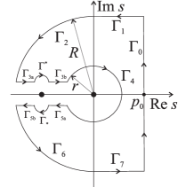
Figure 9: Contour $\Gamma^{\left(\mathrm{II}\right)}.$

The relaxation modulus is obtained in the form

$$\sigma_{sr}\left(t\right)=\frac{1}{\pi}\int_{0}^{\infty}\frac{K\left(\rho\right)}{\left|\Psi\left(\rho\mathrm{e}^{\mathrm{i}\pi}\right)\right|^{2}}\frac{\mathrm{e}^{-\rho t}}{\rho^{1-\mu}}\mathrm{d}\rho+f_{sr}^{\ast}\left(\rho^{\ast}\right)\mathrm{e}^{-\rho^{\ast}t},$$ (179)

with functions $K$ and $f_{sr}^{\ast}$ given by (50) and (71), using the Cauchy integral theorem (178). Namely, the contour $\Gamma_{3a}$ is parametrized by $s=\rho\mathrm{e}^{\mathrm{i}\pi},$ $\rho\in\left(\rho^{\ast}+r^{\ast},R\right),$ while $\Gamma_{3b}$ has the same parametrization with $\rho\in\left(\rho^{\ast}-r^{\ast},r\right)$, so that in the limit when $R\rightarrow\infty,$ $r\rightarrow 0,$ and $r^{\ast}\rightarrow 0$ the integral along contour $\Gamma_{3a}\cup\Gamma_{3b},$ as in (167), reads

$$\lim_{\begin{subarray}{c}R\rightarrow\infty,\\ r\rightarrow 0,\\ r^{\ast}\rightarrow 0\end{subarray}}\int_{\Gamma_{3a}\cup\Gamma_{3b}}\tilde{\sigma}_{sr}\left(s\right)\mathrm{e}^{st}\mathrm{d}s=-\int_{0}^{\infty}\frac{b_{1}+b_{2}\rho^{\eta}\mathrm{e}^{\mathrm{i}\eta\pi}}{\Psi\left(\rho\mathrm{e}^{\mathrm{i}\pi}\right)}\mathrm{e}^{\mathrm{i}\mu\pi}\frac{\mathrm{e}^{-\rho t}}{\rho^{1-\mu}}\mathrm{d}\rho,$$ (180)

and similarly the integral along contour $\Gamma_{5a}\cup\Gamma_{5b}$ (parametrized by $s=\rho\mathrm{e}^{-\mathrm{i}\pi},$ $\rho\in\left(\rho^{\ast}-r^{\ast},r\right)$ for $\Gamma_{5a}$ and $\rho\in\left(\rho^{\ast}+r^{\ast},R\right)$ for $\Gamma_{5b}$), as in (LABEL:int-gama5-1-5), is

$$\lim_{\begin{subarray}{c}R\rightarrow\infty,\\ r\rightarrow 0,\\ r^{\ast}\rightarrow 0\end{subarray}}\int_{\Gamma_{5a}\cup\Gamma_{5b}}\tilde{\sigma}_{sr}\left(s\right)\mathrm{e}^{st}\mathrm{d}s=\int_{0}^{\infty}\frac{b_{1}+b_{2}\rho^{\eta}\mathrm{e}^{-\mathrm{i}\eta\pi}}{\Psi\left(\rho\mathrm{e}^{-\mathrm{i}\pi}\right)}\mathrm{e}^{-\mathrm{i}\mu\pi}\frac{\mathrm{e}^{-\rho t}}{\rho^{1-\mu}}\mathrm{d}\rho,$$ (181)

so that, along with the inverse Laplace transform (169), the integrals in (180) and (181) yield the first term in the relaxation modulus (179), while, as it will be calculated, the integrals along contours $\Gamma^{\ast}$ and $\Gamma_{\ast}$ yield the second term in (179), as the integrals along $\Gamma_{1},$ $\Gamma_{2},$ $\Gamma_{4},$ $\Gamma_{6},$ $\Gamma_{7}$ tend to zero as $R\rightarrow\infty$ and $r\rightarrow 0,$ as already proved in Section B.2.1.

The contour $\Gamma^{\ast}$ is parametrized by $s-\rho^{\ast}\mathrm{e}^{\mathrm{i}\pi}=r^{\ast}\mathrm{e}^{\mathrm{i}\varphi},$ $\varphi\in(0,\pi),$ with $r^{\ast}\rightarrow 0,$ and the corresponding integral reads

$$I_{\Gamma^{\ast}}=\int_{\Gamma^{\ast}}\tilde{\sigma}_{sr}\left(s\right)\mathrm{e}^{st}\mathrm{d}s=\int_{\pi}^{0}\frac{1}{\left(\rho^{\ast}\mathrm{e}^{\mathrm{i}\pi}+r^{\ast}\mathrm{e}^{\mathrm{i}\varphi}\right)^{1-\mu}}\frac{b_{1}+b_{2}\left(\rho^{\ast}\mathrm{e}^{\mathrm{i}\pi}+r^{\ast}\mathrm{e}^{\mathrm{i}\varphi}\right)^{\eta}}{\Psi\left(\rho^{\ast}\mathrm{e}^{\mathrm{i}\pi}+r^{\ast}\mathrm{e}^{\mathrm{i}\varphi}\right)}\mathrm{e}^{\left(\rho^{\ast}\mathrm{e}^{\mathrm{i}\pi}+r^{\ast}\mathrm{e}^{\mathrm{i}\varphi}\right)t}\mathrm{i}r^{\ast}\mathrm{e}^{\mathrm{i}\varphi}\mathrm{d}\varphi,$$

so that by letting $r^{\ast}\rightarrow 0$ in the previous expression one obtains

$$\lim_{{}_{\begin{subarray}{c}r^{\ast}\rightarrow 0\end{subarray}}}I_{\Gamma^{\ast}} = -\mathrm{i}\frac{b_{1}+b_{2}\left(\rho^{\ast}\right)^{\eta}\mathrm{e}^{\mathrm{i}\eta\pi}}{\left(\rho^{\ast}\right)^{1-\mu}\mathrm{e}^{\mathrm{i}\left(1-\mu\right)\pi}}\mathrm{e}^{-\rho^{\ast}t}\lim_{{}_{\begin{subarray}{c}r^{\ast}\rightarrow 0\end{subarray}}}\int_{0}^{\pi}\frac{r^{\ast}\mathrm{e}^{\mathrm{i}\varphi}}{\Psi\left(\rho^{\ast}\mathrm{e}^{\mathrm{i}\pi}+r^{\ast}\mathrm{e}^{\mathrm{i}\varphi}\right)}\mathrm{d}\varphi,$$ (182)

$$= -\mathrm{i}\pi\left(\rho^{\ast}\right)^{\mu}\mathrm{e}^{\mathrm{i}\mu\pi}\frac{b_{1}+b_{2}\left(\rho^{\ast}\right)^{\eta}\mathrm{e}^{\mathrm{i}\eta\pi}}{\alpha a_{1}\left(\rho^{\ast}\right)^{\alpha}\mathrm{e}^{\mathrm{i}\alpha\pi}+\beta a_{2}\left(\rho^{\ast}\right)^{\beta}\mathrm{e}^{\mathrm{i}\beta\pi}+\gamma a_{3}\left(\rho^{\ast}\right)^{\gamma}\mathrm{e}^{\mathrm{i}\gamma\pi}}\mathrm{e}^{-\rho^{\ast}t}.$$

In calculating (182), function $\Psi$ (38) for $r^{\ast}\rightarrow 0$ is written as

$$\Psi\left(\rho^{\ast}\mathrm{e}^{\mathrm{i}\pi}+r^{\ast}\mathrm{e}^{\mathrm{i}\varphi}\right)\!\!\!\! = \!\!\!\!1+a_{1}\left(\rho^{\ast}\right)^{\alpha}\mathrm{e}^{\mathrm{i}\alpha\pi}\left(1-\frac{r^{\ast}\mathrm{e}^{\mathrm{i}\varphi}}{\rho^{\ast}}\right)^{\alpha}+a_{2}\left(\rho^{\ast}\right)^{\beta}\mathrm{e}^{\mathrm{i}\beta\pi}\left(1-\frac{r^{\ast}\mathrm{e}^{\mathrm{i}\varphi}}{\rho^{\ast}}\right)^{\beta}+a_{3}\left(\rho^{\ast}\right)^{\gamma}\mathrm{e}^{\mathrm{i}\gamma\pi}\left(1-\frac{r^{\ast}\mathrm{e}^{\mathrm{i}\varphi}}{\rho^{\ast}}\right)^{\gamma}$$ (183)

$$\approx \!\!\!\!1+a_{1}\left(\rho^{\ast}\right)^{\alpha}\mathrm{e}^{\mathrm{i}\alpha\pi}\left(1-\alpha\frac{r^{\ast}\mathrm{e}^{\mathrm{i}\varphi}}{\rho^{\ast}}\right)+a_{2}\left(\rho^{\ast}\right)^{\beta}\mathrm{e}^{\mathrm{i}\beta\pi}\left(1-\beta\frac{r^{\ast}\mathrm{e}^{\mathrm{i}\varphi}}{\rho^{\ast}}\right)+a_{3}\left(\rho^{\ast}\right)^{\gamma}\mathrm{e}^{\mathrm{i}\gamma\pi}\left(1-\gamma\frac{r^{\ast}\mathrm{e}^{\mathrm{i}\varphi}}{\rho^{\ast}}\right)$$

$$\approx \!\!\!\!-\frac{r^{\ast}\mathrm{e}^{\mathrm{i}\varphi}}{\rho^{\ast}}\left(\alpha a_{1}\left(\rho^{\ast}\right)^{\alpha}\mathrm{e}^{\mathrm{i}\alpha\pi}+\beta a_{2}\left(\rho^{\ast}\right)^{\beta}\mathrm{e}^{\mathrm{i}\beta\pi}+\gamma a_{3}\left(\rho^{\ast}\right)^{\gamma}\mathrm{e}^{\mathrm{i}\gamma\pi}\right),$$

where the approximation $\left(1+x\right)^{\xi}\approx 1+\xi x,$ for $\left|x\right|\ll 1,$ and fact that $\Psi\left(\rho^{\ast}\mathrm{e}^{\mathrm{i}\pi}\right)=0$ (since $\rho^{\ast}$ is negative real zero of $\Psi$) are used, implying

$$\lim_{{}_{\begin{subarray}{c}r^{\ast}\rightarrow 0\end{subarray}}}\frac{r^{\ast}\mathrm{e}^{\mathrm{i}\varphi}}{\Psi\left(\rho^{\ast}\mathrm{e}^{\mathrm{i}\pi}+r^{\ast}\mathrm{e}^{\mathrm{i}\varphi}\right)}=-\frac{\rho^{\ast}}{\alpha a_{1}\left(\rho^{\ast}\right)^{\alpha}\mathrm{e}^{\mathrm{i}\alpha\pi}+\beta a_{2}\left(\rho^{\ast}\right)^{\beta}\mathrm{e}^{\mathrm{i}\beta\pi}+\gamma a_{3}\left(\rho^{\ast}\right)^{\gamma}\mathrm{e}^{\mathrm{i}\gamma\pi}}.$$ (184)

The integral corresponding to contour $\Gamma_{\ast}$, parametrized by $s-\rho^{\ast}\mathrm{e}^{-\mathrm{i}\pi}=r^{\ast}\mathrm{e}^{\mathrm{i}\varphi},$ $\varphi\in(-\pi,0),$ in the limit when $r^{\ast}\rightarrow 0$ is obtained as

$$\lim_{{}_{\begin{subarray}{c}r^{\ast}\rightarrow 0\end{subarray}}}I_{\Gamma_{\ast}} = \lim_{{}_{\begin{subarray}{c}r^{\ast}\rightarrow 0\end{subarray}}}\int_{\Gamma_{\ast}}\tilde{\sigma}_{sr}\left(s\right)\mathrm{e}^{st}\mathrm{d}s$$

$$= \mathrm{i}\frac{b_{1}+b_{2}\left(\rho^{\ast}\right)^{\eta}\mathrm{e}^{-\mathrm{i}\eta\pi}}{\left(\rho^{\ast}\right)^{1-\mu}\mathrm{e}^{-\mathrm{i}\left(1-\mu\right)\pi}}\mathrm{e}^{-\rho^{\ast}t}\lim_{{}_{\begin{subarray}{c}r^{\ast}\rightarrow 0\end{subarray}}}\int_{0}^{-\pi}\frac{r^{\ast}\mathrm{e}^{\mathrm{i}\varphi}}{\Psi\left(\rho^{\ast}\mathrm{e}^{-\mathrm{i}\pi}+r^{\ast}\mathrm{e}^{\mathrm{i}\varphi}\right)}\mathrm{d}\varphi$$

$$= -\mathrm{i}\pi\left(\rho^{\ast}\right)^{\mu}\mathrm{e}^{-\mathrm{i}\mu\pi}\frac{b_{1}+b_{2}\left(\rho^{\ast}\right)^{\eta}\mathrm{e}^{-\mathrm{i}\eta\pi}}{\alpha a_{1}\left(\rho^{\ast}\right)^{\alpha}\mathrm{e}^{-\mathrm{i}\alpha\pi}+\beta a_{2}\left(\rho^{\ast}\right)^{\beta}\mathrm{e}^{-\mathrm{i}\beta\pi}+\gamma a_{3}\left(\rho^{\ast}\right)^{\gamma}\mathrm{e}^{-\mathrm{i}\gamma\pi}}\mathrm{e}^{-\rho^{\ast}t},$$

using the similar procedure as in calculating $\lim_{{}_{\begin{subarray}{c}r^{\ast}\rightarrow 0\end{subarray}}}I_{\Gamma^{\ast}}$.

Therefore, one has

$$\lim_{{}_{\begin{subarray}{c}r^{\ast}\rightarrow 0\end{subarray}}}\left(I_{\Gamma^{\ast}}+I_{\Gamma_{\ast}}\right) = -\mathrm{i}\pi\left(\frac{b_{1}+b_{2}\left(\rho^{\ast}\right)^{\eta}\mathrm{e}^{\mathrm{i}\eta\pi}}{\alpha a_{1}\left(\rho^{\ast}\right)^{\alpha}\mathrm{e}^{\mathrm{i}\alpha\pi}+\beta a_{2}\left(\rho^{\ast}\right)^{\beta}\mathrm{e}^{\mathrm{i}\beta\pi}+\gamma a_{3}\left(\rho^{\ast}\right)^{\gamma}\mathrm{e}^{\mathrm{i}\gamma\pi}}\mathrm{e}^{\mathrm{i}\mu\pi}\right.$$

$$+\left.\frac{b_{1}+b_{2}\left(\rho^{\ast}\right)^{\eta}\mathrm{e}^{-\mathrm{i}\eta\pi}}{\alpha a_{1}\left(\rho^{\ast}\right)^{\alpha}\mathrm{e}^{-\mathrm{i}\alpha\pi}+\beta a_{2}\left(\rho^{\ast}\right)^{\beta}\mathrm{e}^{-\mathrm{i}\beta\pi}+\gamma a_{3}\left(\rho^{\ast}\right)^{\gamma}\mathrm{e}^{-\mathrm{i}\gamma\pi}}\mathrm{e}^{-\mathrm{i}\mu\pi}\right)\left(\rho^{\ast}\right)^{\mu}\mathrm{e}^{-\rho^{\ast}t},$$

yielding function $f_{sr}^{\ast}$ in the form (71) and representing the second term in (179).

Relaxation modulus in the case of models having non-zero glass compliance. Inverting the Laplace transform in the relaxation modulus in complex domain (57), one obtains

$$\sigma_{sr}\left(t\right) = \frac{b_{2}}{a_{3}}-\frac{b_{2}}{a_{3}}\int_{0}^{t}\mathcal{L}^{-1}\left[\tilde{f}_{sr}\left(s\right)\right]\left(\tau\right)\mathrm{d}\tau$$ (185)

$$= \frac{b_{2}}{a_{3}}-\frac{b_{2}}{a_{3}}\int_{0}^{t}f_{sr}\left(\tau\right)\mathrm{d}\tau+\frac{b_{2}}{a_{3}}f_{sr}^{\ast}\left(\rho^{\ast}\right)\left(1-\mathrm{e}^{-\rho^{\ast}t}\right),$$

where functions $\tilde{f}_{sr},$ $f_{sr},$ and $f_{sr}^{\ast}$ are respectively given by (172), (74), and (79), due to the existence of negative real zero $-\rho^{\ast}$ of function $\Psi$ (38), with $\rho^{\ast}$ determined from (70) with $\gamma=\beta+\eta.$ Namely, using function $\tilde{f}_{sr}$ in the form

$$\tilde{f}_{sr}\left(s\right)=\frac{\psi\left(s\right)}{\psi\left(s\right)+s^{\beta}\left(\frac{b_{1}}{b_{2}}+s^{\eta}\right)}=\frac{1+a_{1}s^{\alpha}+a_{3}\left(\frac{a_{2}}{a_{3}}-\frac{b_{1}}{b_{2}}\right)s^{\beta}}{\Psi\left(s\right)},$$ (186)

see (39) and (38), as an integrand in the Cauchy integral theorem

$$\oint_{\Gamma^{\left(\mathrm{II}\right)}}\tilde{f}_{sr}\left(s\right)\mathrm{e}^{st}\mathrm{d}s=0,$$ (187)

where the contour $\Gamma^{\left(\mathrm{II}\right)}=\Gamma_{0}\cup\Gamma_{1}\cup\Gamma_{2}\cup\Gamma_{3a}\cup\Gamma^{\ast}\cup\Gamma_{3b}\cup\Gamma_{4}\cup\Gamma_{5a}\cup\Gamma_{\ast}\cup\Gamma_{5b}\cup\Gamma_{6}\cup\Gamma_{7}$ is chosen as in Figure 9, one obtains the second and third term in (185).

The contour $\Gamma_{3a}$ is parametrized by $s=\rho\mathrm{e}^{\mathrm{i}\pi},$ $\rho\in\left(\rho^{\ast}+r^{\ast},R\right),$ while $\Gamma_{3b}$ has the same parametrization with $\rho\in\left(\rho^{\ast}-r^{\ast},r\right)$, so that in the limit when $R\rightarrow\infty,$ $r\rightarrow 0$ and $r^{\ast}\rightarrow 0$ the integral along contour $\Gamma_{3a}\cup\Gamma_{3b},$ as in (174), reads

$$\lim_{\begin{subarray}{c}R\rightarrow\infty,\\ r\rightarrow 0,\\ r^{\ast}\rightarrow 0\end{subarray}}\int_{\Gamma_{3a}\cup\Gamma_{3b}}\tilde{f}_{sr}\left(s\right)\mathrm{e}^{st}\mathrm{d}s=\int_{0}^{\infty}\frac{\psi\left(\rho\mathrm{e}^{\mathrm{i}\pi}\right)}{\psi\left(\rho\mathrm{e}^{\mathrm{i}\pi}\right)+\rho^{\beta}\mathrm{e}^{\mathrm{i}\beta\pi}\left(\frac{b_{1}}{b_{2}}+\rho^{\eta}\mathrm{e}^{\mathrm{i}\eta\pi}\right)}\mathrm{e}^{-\rho t}\mathrm{d}\rho.$$ (188)

Similarly, the integral along contour $\Gamma_{5a}\cup\Gamma_{5b}$ (parametrized by $s=\rho\mathrm{e}^{-\mathrm{i}\pi},$ $\rho\in\left(\rho^{\ast}-r^{\ast},r\right)$ for $\Gamma_{5a}$ and $\rho\in\left(\rho^{\ast}+r^{\ast},R\right)$ for $\Gamma_{5b}$), as in (175), is

$$\lim_{{}_{\begin{subarray}{c}R\rightarrow\infty,\\ r\rightarrow 0,\\ r^{\ast}\rightarrow 0\end{subarray}}}\int_{\Gamma_{5a}\cup\Gamma_{5b}}\tilde{f}_{sr}\left(s\right)\mathrm{e}^{st}\mathrm{d}s=-\int_{0}^{\infty}\frac{\psi\left(\rho\mathrm{e}^{-\mathrm{i}\pi}\right)}{\psi\left(\rho\mathrm{e}^{-\mathrm{i}\pi}\right)+\rho^{\beta}\mathrm{e}^{-\mathrm{i}\beta\pi}\left(\frac{b_{1}}{b_{2}}+\rho^{\eta}\mathrm{e}^{-\mathrm{i}\eta\pi}\right)}\mathrm{e}^{-\rho t}\mathrm{d}\rho.$$ (189)

The contour $\Gamma^{\ast}$ is parametrized by $s-\rho^{\ast}\mathrm{e}^{\mathrm{i}\pi}=r^{\ast}\mathrm{e}^{\mathrm{i}\varphi},$ $\varphi\in(0,\pi),$ with $r^{\ast}\rightarrow 0,$ so that the corresponding integral reads

$$I_{\Gamma^{\ast}} = \int_{\Gamma^{\ast}}\tilde{f}_{sr}\left(s\right)\mathrm{e}^{st}\mathrm{d}s$$

$$= \int_{\pi}^{0}\frac{1+a_{1}\left(\rho^{\ast}\mathrm{e}^{\mathrm{i}\pi}+r^{\ast}\mathrm{e}^{\mathrm{i}\varphi}\right)^{\alpha}+a_{3}\left(\frac{a_{2}}{a_{3}}-\frac{b_{1}}{b_{2}}\right)\left(\rho^{\ast}\mathrm{e}^{\mathrm{i}\pi}+r^{\ast}\mathrm{e}^{\mathrm{i}\varphi}\right)^{\beta}}{\Psi\left(\rho^{\ast}\mathrm{e}^{\mathrm{i}\pi}+r^{\ast}\mathrm{e}^{\mathrm{i}\varphi}\right)}\mathrm{e}^{\left(\rho^{\ast}\mathrm{e}^{\mathrm{i}\pi}+r^{\ast}\mathrm{e}^{\mathrm{i}\varphi}\right)t}\mathrm{i}r^{\ast}\mathrm{e}^{\mathrm{i}\varphi}\mathrm{d}\varphi,$$

so that by letting $r^{\ast}\rightarrow 0$ in the previous expression one obtains

$$\lim_{{}_{\begin{subarray}{c}r^{\ast}\rightarrow 0\end{subarray}}}I_{\Gamma^{\ast}} = -\mathrm{i}\left(1+a_{1}\left(\rho^{\ast}\right)^{\alpha}\mathrm{e}^{\mathrm{i}\alpha\pi}+a_{3}\left(\frac{a_{2}}{a_{3}}-\frac{b_{1}}{b_{2}}\right)\left(\rho^{\ast}\right)^{\beta}\mathrm{e}^{\mathrm{i}\beta\pi}\right)\mathrm{e}^{-\rho^{\ast}t}\lim_{{}_{\begin{subarray}{c}r^{\ast}\rightarrow 0\end{subarray}}}\int_{0}^{\pi}\frac{r^{\ast}\mathrm{e}^{\mathrm{i}\varphi}}{\Psi\left(\rho^{\ast}\mathrm{e}^{\mathrm{i}\pi}+r^{\ast}\mathrm{e}^{\mathrm{i}\varphi}\right)}\mathrm{d}\varphi,$$ (190)

$$= \mathrm{i}\pi\frac{1+a_{1}\left(\rho^{\ast}\right)^{\alpha}\mathrm{e}^{\mathrm{i}\alpha\pi}+a_{3}\left(\frac{a_{2}}{a_{3}}-\frac{b_{1}}{b_{2}}\right)\left(\rho^{\ast}\right)^{\beta}\mathrm{e}^{\mathrm{i}\beta\pi}}{\alpha a_{1}\left(\rho^{\ast}\right)^{\alpha}\mathrm{e}^{\mathrm{i}\alpha\pi}+\beta a_{2}\left(\rho^{\ast}\right)^{\beta}\mathrm{e}^{\mathrm{i}\beta\pi}+\left(\beta+\eta\right)a_{3}\left(\rho^{\ast}\right)^{\beta+\eta}\mathrm{e}^{\mathrm{i}\left(\beta+\eta\right)\pi}}\rho^{\ast}\mathrm{e}^{-\rho^{\ast}t}.$$

In calculating (190), the expression (184), with $\gamma=\beta+\eta,$ is used. The integral corresponding to contour $\Gamma_{\ast}$, parametrized by $s-\rho^{\ast}\mathrm{e}^{-\mathrm{i}\pi}=r^{\ast}\mathrm{e}^{\mathrm{i}\varphi},$ $\varphi\in(-\pi,0),$ in the limit when $r^{\ast}\rightarrow 0$ reads

$$\lim_{{}_{\begin{subarray}{c}r^{\ast}\rightarrow 0\end{subarray}}}I_{\Gamma_{\ast}} = \lim_{{}_{\begin{subarray}{c}r^{\ast}\rightarrow 0\end{subarray}}}\int_{\Gamma_{\ast}}\tilde{f}_{sr}\left(s\right)\mathrm{e}^{st}\mathrm{d}s$$ (191)

$$= \mathrm{i}\left(1+a_{1}\left(\rho^{\ast}\right)^{\alpha}\mathrm{e}^{-\mathrm{i}\alpha\pi}+a_{3}\left(\frac{a_{2}}{a_{3}}-\frac{b_{1}}{b_{2}}\right)\left(\rho^{\ast}\right)^{\beta}\mathrm{e}^{-\mathrm{i}\beta\pi}\right)\mathrm{e}^{-\rho^{\ast}t}\lim_{{}_{\begin{subarray}{c}r^{\ast}\rightarrow 0\end{subarray}}}\int_{0}^{-\pi}\frac{r^{\ast}\mathrm{e}^{\mathrm{i}\varphi}}{\Psi\left(\rho^{\ast}\mathrm{e}^{-\mathrm{i}\pi}+r^{\ast}\mathrm{e}^{\mathrm{i}\varphi}\right)}\mathrm{d}\varphi$$

$$= \mathrm{i}\pi\frac{1+a_{1}\left(\rho^{\ast}\right)^{\alpha}\mathrm{e}^{-\mathrm{i}\alpha\pi}+a_{3}\left(\frac{a_{2}}{a_{3}}-\frac{b_{1}}{b_{2}}\right)\left(\rho^{\ast}\right)^{\beta}\mathrm{e}^{-\mathrm{i}\beta\pi}}{\alpha a_{1}\left(\rho^{\ast}\right)^{\alpha}\mathrm{e}^{-\mathrm{i}\alpha\pi}+\beta a_{2}\left(\rho^{\ast}\right)^{\beta}\mathrm{e}^{-\mathrm{i}\beta\pi}+\left(\beta+\eta\right)a_{3}\left(\rho^{\ast}\right)^{\beta+\eta}\mathrm{e}^{-\mathrm{i}\left(\beta+\eta\right)\pi}}\rho^{\ast}\mathrm{e}^{-\rho^{\ast}t},$$

using the similar procedure as in calculating $\lim_{{}_{\begin{subarray}{c}r^{\ast}\rightarrow 0\end{subarray}}}I_{\Gamma^{\ast}}$.

In the limit when $R\rightarrow\infty,$ $r\rightarrow 0,$ and $r^{\ast}\rightarrow 0,$ the inverse Laplace transform $\mathcal{L}^{-1}\left[\tilde{f}_{sr}\left(s\right)\right]$ (173), i.e., the second and the third term in the relaxation modulus (185), is obtained from the Cauchy integral theorem (187) as the sum of integrals along contours $\Gamma_{3a}\cup\Gamma_{3b},$ $\Gamma_{5a}\cup\Gamma_{5b},$ $\Gamma^{\ast},$ and $\Gamma_{\ast},$ respectively given by (188), (189), (190), and (191), since the integrals along $\Gamma_{1},$ $\Gamma_{2},$ $\Gamma_{4},$ $\Gamma_{6},$ $\Gamma_{7}$ tend to zero as $R\rightarrow\infty$ and $r\rightarrow 0,$ as already proved in Section B.2.1. Therefore, one has

$$\mathcal{L}^{-1}\left[\tilde{f}_{sr}\left(s\right)\right]\left(t\right)=f_{sr}\left(t\right)-\rho^{\ast}f_{sr}^{\ast}\left(\rho^{\ast}\right)\mathrm{e}^{-\rho^{\ast}t},$$

with $f_{sr}$ given by (74) and

$$f_{sr}^{\ast}\left(\rho^{\ast}\right) = \frac{1}{2}\left(\frac{1+a_{1}\left(\rho^{\ast}\right)^{\alpha}\mathrm{e}^{\mathrm{i}\alpha\pi}+a_{3}\left(\frac{a_{2}}{a_{3}}-\frac{b_{1}}{b_{2}}\right)\left(\rho^{\ast}\right)^{\beta}\mathrm{e}^{\mathrm{i}\beta\pi}}{\alpha a_{1}\left(\rho^{\ast}\right)^{\alpha}\mathrm{e}^{\mathrm{i}\alpha\pi}+\beta a_{2}\left(\rho^{\ast}\right)^{\beta}\mathrm{e}^{\mathrm{i}\beta\pi}+\left(\beta+\eta\right)a_{3}\left(\rho^{\ast}\right)^{\beta+\eta}\mathrm{e}^{\mathrm{i}\left(\beta+\eta\right)\pi}}\right.$$

$$+\left.\frac{1+a_{1}\left(\rho^{\ast}\right)^{\alpha}\mathrm{e}^{-\mathrm{i}\alpha\pi}+a_{3}\left(\frac{a_{2}}{a_{3}}-\frac{b_{1}}{b_{2}}\right)\left(\rho^{\ast}\right)^{\beta}\mathrm{e}^{-\mathrm{i}\beta\pi}}{\alpha a_{1}\left(\rho^{\ast}\right)^{\alpha}\mathrm{e}^{-\mathrm{i}\alpha\pi}+\beta a_{2}\left(\rho^{\ast}\right)^{\beta}\mathrm{e}^{-\mathrm{i}\beta\pi}+\left(\beta+\eta\right)a_{3}\left(\rho^{\ast}\right)^{\beta+\eta}\mathrm{e}^{-\mathrm{i}\left(\beta+\eta\right)\pi}}\right),$$

yielding (79).

B.2.3 Case when function $\Psi$ has a pair of complex conjugated zeros

Relaxation modulus in the case of models having zero glass compliance. The Cauchy residue theorem with the relaxation modulus in complex domain (56) as an integrand takes the form

$$\oint_{\Gamma^{\left(\mathrm{I}\right)}}\tilde{\sigma}_{sr}\left(s\right)\mathrm{e}^{st}\mathrm{d}s=2\pi\mathrm{i}\left(\mathop{\mathrm{R}es}\left(\tilde{\sigma}_{sr}\left(s\right)\mathrm{e}^{st},s_{0}\right)+\mathop{\mathrm{R}es}\left(\tilde{\sigma}_{sr}\left(s\right)\mathrm{e}^{st},\bar{s}_{0}\right)\right),$$ (192)

due to the existence of complex conjugated zeroes $s_{0}$ and $\bar{s}_{0}$ having negative real part of function $\Psi,$ given by (38), with the contour $\Gamma^{\left(\mathrm{I}\right)}=\Gamma_{0}\cup\Gamma_{1}\cup\Gamma_{2}\cup\Gamma_{3}\cup\Gamma_{4}\cup\Gamma_{5}\cup\Gamma_{6}\cup\Gamma_{7}$ chosen as in Figure 8.

The relaxation modulus is obtained in the form

$$\sigma_{sr}\left(t\right)=\frac{1}{\pi}\int_{0}^{\infty}\frac{K\left(\rho\right)}{\left|\Psi\left(\rho\mathrm{e}^{\mathrm{i}\pi}\right)\right|^{2}}\frac{\mathrm{e}^{-\rho t}}{\rho^{1-\mu}}\mathrm{d}\rho+f_{sr}^{\left(r\right)}\left(t\right),$$ (193)

with functions $K$ and $f_{sr}^{\left(r\right)}$ given by (50) and (72), using the Cauchy residue theorem (192). Namely, the integration along the contour $\Gamma^{\left(\mathrm{I}\right)}$ yields the inverse Laplace transform (169) and the first term in the relaxation modulus (193), that is already obtained in Section B.2.1, while the second term in (193) consists of the residues of function $\tilde{\sigma}_{sr}\left(s\right)\mathrm{e}^{st},$ since $s_{0}=\rho_{0}\mathrm{e}^{\mathrm{i}\varphi_{0}}$ and $\bar{s}_{0}=\rho_{0}\mathrm{e}^{-\mathrm{i}\varphi_{0}},$ $\varphi_{0}\in\left(\frac{\pi}{2},\pi\right),$ are its poles of the first order, i.e., the first order zeros of function $\Psi$ (38). Therefore, one has

$$f_{sr}^{\left(r\right)}\left(t\right) = \left[\frac{1}{s^{1-\mu}}\frac{b_{1}+b_{2}s^{\eta}}{\frac{\mathrm{d}}{\mathrm{d}s}\Psi\left(s\right)}\mathrm{e}^{st}\right]_{s=s_{0}}+\left[\frac{1}{s^{1-\mu}}\frac{b_{1}+b_{2}s^{\eta}}{\frac{\mathrm{d}}{\mathrm{d}s}\Psi\left(s\right)}\mathrm{e}^{st}\right]_{s=\bar{s}_{0}}$$

$$= \left(\left.\frac{b_{1}+b_{2}s^{\eta}}{\alpha a_{1}s^{\alpha-1}+\beta a_{2}s^{\beta-1}+\gamma a_{3}s^{\gamma-1}}\right|_{s=\rho_{0}\mathrm{e}^{\mathrm{i}\varphi_{0}}}\frac{\mathrm{e}^{-\mathrm{i}\left(1-\mu\right)\varphi_{0}}}{\rho_{0}^{1-\mu}}\mathrm{e}^{\mathrm{i}\rho_{0}t\sin\varphi_{0}}\right.$$

$$+\left.\left.\frac{b_{1}+b_{2}s^{\eta}}{\alpha a_{1}s^{\alpha-1}+\beta a_{2}s^{\beta-1}+\gamma a_{3}s^{\gamma-1}}\right|_{s=\rho_{0}\mathrm{e}^{-\mathrm{i}\varphi_{0}}}\frac{\mathrm{e}^{\mathrm{i}\left(1-\mu\right)\varphi_{0}}}{\rho_{0}^{1-\mu}}\mathrm{e}^{\mathrm{i}\rho_{0}t\sin\varphi_{0}}\right)\mathrm{e}^{\rho_{0}t\cos\varphi_{0}},$$

yielding (72).

Relaxation modulus in the case of models having non-zero glass compliance. Inverting the Laplace transform in the relaxation modulus in complex domain (57), one obtains

$$\sigma_{sr}\left(t\right) = \frac{b_{2}}{a_{3}}-\frac{b_{2}}{a_{3}}\int_{0}^{t}\mathcal{L}^{-1}\left[\tilde{f}_{sr}\left(s\right)\right]\left(\tau\right)\mathrm{d}\tau$$ (194)

$$= \frac{b_{2}}{a_{3}}-\frac{b_{2}}{a_{3}}\int_{0}^{t}f_{sr}\left(\tau\right)\mathrm{d}\tau-\frac{b_{2}}{a_{3}}\int_{0}^{t}f_{sr}^{\left(r\right)}\left(\tau\right)\mathrm{d}\tau,$$

where functions $\tilde{f}_{sr},$ $f_{sr},$ and $f_{sr}^{\left(r\right)}$ are respectively given by (172), (74), and (80), due to the existence of complex conjugated zeroes $s_{0}$ and $\bar{s}_{0}$ of function $\Psi$ (38) having negative real part.

Using function $\tilde{f}_{sr}$ in the form (186) as an integrand in the Cauchy residue theorem

$$\oint_{\Gamma^{\left(\mathrm{I}\right)}}\tilde{f}_{sr}\left(s\right)\mathrm{e}^{st}\mathrm{d}s=2\pi\mathrm{i}\left(\mathop{\mathrm{R}es}\left(\tilde{f}_{sr}\left(s\right)\mathrm{e}^{st},s_{0}\right)+\mathop{\mathrm{R}es}\left(\tilde{f}_{sr}\left(s\right)\mathrm{e}^{st},\bar{s}_{0}\right)\right),$$

with the contour $\Gamma^{\left(\mathrm{I}\right)}=\Gamma_{0}\cup\Gamma_{1}\cup\Gamma_{2}\cup\Gamma_{3}\cup\Gamma_{4}\cup\Gamma_{5}\cup\Gamma_{6}\cup\Gamma_{7}$ chosen as in Figure 8, one obtains the inverse Laplace transform $\mathcal{L}^{-1}\left[\tilde{f}_{sr}\left(s\right)\right]$ (173), i.e., the second and the third term in (194), in the form

$$\mathcal{L}^{-1}\left[\tilde{f}_{sr}\left(s\right)\right]\left(t\right)=f_{sr}\left(t\right)+f_{sr}^{\left(r\right)}\left(t\right).$$ (195)

The first term in (195), being a consequence of the integration along the contour $\Gamma^{\left(\mathrm{I}\right)},$ is already obtained in Section B.2.1, while the second one consists of the residues of function $\tilde{f}_{sr}\left(s\right)\mathrm{e}^{st},$ since $s_{0}=\rho_{0}\mathrm{e}^{\mathrm{i}\varphi_{0}}$ and $\bar{s}_{0}=\rho_{0}\mathrm{e}^{-\mathrm{i}\varphi_{0}},$ $\varphi_{0}\in\left(\frac{\pi}{2},\pi\right),$ are its poles of the first order, i.e., the first order zeros of function $\Psi,$ as proved in Section A.1. Therefore in (195), one has $f_{sr}$ given by (74) and

$$f_{sr}^{\left(r\right)}\left(t\right) = \left[\frac{1+a_{1}s^{\alpha}+a_{3}\left(\frac{a_{2}}{a_{3}}-\frac{b_{1}}{b_{2}}\right)s^{\beta}}{\frac{\mathrm{d}}{\mathrm{d}s}\Psi\left(s\right)}\mathrm{e}^{st}\right]_{s=s_{0}}+\left[\frac{1+a_{1}s^{\alpha}+a_{3}\left(\frac{a_{2}}{a_{3}}-\frac{b_{1}}{b_{2}}\right)s^{\beta}}{\frac{\mathrm{d}}{\mathrm{d}s}\Psi\left(s\right)}\mathrm{e}^{st}\right]_{s=\bar{s}_{0}}$$

$$= \left(\left.\frac{1+a_{1}s^{\alpha}+a_{3}\left(\frac{a_{2}}{a_{3}}-\frac{b_{1}}{b_{2}}\right)s^{\beta}}{\alpha a_{1}s^{\alpha-1}+\beta a_{2}s^{\beta-1}+\left(\beta+\eta\right)a_{3}s^{\beta+\eta-1}}\right|_{s=\rho_{0}\mathrm{e}^{\mathrm{i}\varphi_{0}}}\mathrm{e}^{\mathrm{i}\rho_{0}t\sin\varphi_{0}}\right.$$

$$+\left.\left.\frac{1+a_{1}s^{\alpha}+a_{3}\left(\frac{a_{2}}{a_{3}}-\frac{b_{1}}{b_{2}}\right)s^{\beta}}{\alpha a_{1}s^{\alpha-1}+\beta a_{2}s^{\beta-1}+\left(\beta+\eta\right)a_{3}s^{\beta+\eta-1}}\right|_{s=\rho_{0}\mathrm{e}^{-\mathrm{i}\varphi_{0}}}\mathrm{e}^{-\mathrm{i}\rho_{0}t\sin\varphi_{0}}\right)\mathrm{e}^{\rho_{0}t\cos\varphi_{0}},$$

yielding (80).

References

- [1] T. M. Atanackovic, S. Pilipovic, B. Stankovic, and D. Zorica. Fractional Calculus with Applications in Mechanics: Vibrations and Diffusion Processes. Wiley-ISTE, London, 2014.
- [2] T. M. Atanackovic, S. Pilipovic, B. Stankovic, and D. Zorica. Fractional Calculus with Applications in Mechanics: Wave Propagation, Impact and Variational Principles. Wiley-ISTE, London, 2014.
- [3] T. M. Atanackovic, S. Pilipovic, and D. Zorica. Distributed-order fractional wave equation on a finite domain: creep and forced oscillations of a rod. Continuum Mechanics and Thermodynamics, 23:305–318, 2011.
- [4] T. M. Atanackovic, S. Pilipovic, and D. Zorica. Distributed-order fractional wave equation on a finite domain. Stress relaxation in a rod. International Journal of Engineering Science, 49:175–190, 2011.
- [5] R. L. Bagley and P. J. Torvik. On the fractional calculus model of viscoelastic behavior. Journal of Rheology, 30:133–155, 1986.
- [6] E. Bazhlekova and I. Bazhlekov. Complete monotonicity of the relaxation moduli of distributed-order fractional Zener model. In Proceedings of the 44 International Conference on Applications of Mathematics in Engineering and Economics, AIP Conference Proceedings 2048, pages 050008–1–8, 2018.
- [7] E. Bazhlekova and K. Tsocheva. Fractional Burgers’ model: thermodynamic constraints and completely monotonic relaxation function. Comptes rendus de l’Académie bulgare des Sciences, 69:825–834, 2016.
- [8] C. Celauro, C. Fecarotti, A. Pirrotta, and A. C. Collop. Experimental validation of a fractional model for creep/recovery testing of asphalt mixtures. Construction and Building Materials, 36:458–466, 2012.
- [9] W. N. Findley, J. S. Lai, and K. Onaran. Creep and Relaxation of Nonlinear Viscoelastic Materials - With an Introduction to Linear Viscoelasticity. Dover Publications, New York, 1976.
- [10] R. Gorenflo and F. Mainardi. Fractional Calculus: Integral and Differential Equations of Fractional Order. In: Fractals and Fractional Calculus in Continuum Mechanics (eds A. Carpinteri, F. Mainardi), volume 378 of CISM Courses and Lecture Notes. Springer Verlag, Wien and New York, 1997.
- [11] A. A. Kilbas, H. M. Srivastava, and J. J. Trujillo. Theory and Applications of Fractional Differential Equations. Elsevier B.V., Amsterdam, 2006.
- [12] F. Mainardi. Fractional Calculus and Waves in Linear Viscoelasticity. Imperial College Press, London, 2010.
- [13] F. Mainardi and G. Spada. Creep, relaxation and viscosity properties for basic fractional models in rheology. European Physical Journal Special Topics, 193:133–160, 2011.
- [14] N. Makris. The frequency response function of the creep compliance. Meccanica, 2018.
- [15] M. Oeser, T. Pellinen, T. Scarpas, and C. Kasbergen. Studies on creep and recovery of rheological bodies based upon conventional and fractional formulations and their application on asphalt mixture. International Journal of Pavement Engineering, 9:373–386, 2008.
- [16] A. S. Okuka and D. Zorica. Formulation of thermodynamically consistent fractional Burgers models. Acta Mechanica, 229:3557–3570, 2018.
- [17] Yu. A. Rossikhin and M. V. Shitikova. Analysis of rheological equations involving more than one fractional parameters by the use of the simplest mechanical systems based on these equations. Mechanics of Time-Dependent Materials, 5:131–175, 2001.
- [18] Yu. A. Rossikhin and M. V. Shitikova. Analysis of the viscoelastic rod dynamics via models involving fractional derivatives or operators of two different orders. Shock and Vibration Digest, 36:3–26, 2004.
- [19] Yu. A. Rossikhin and M. V. Shitikova. Free damped vibrations of a viscoelastic oscillator based on Rabotnov’s model. Mechanics of Time-Dependent Materials, 12:129–149, 2008.
- [20] A. Zbiciak. Mathematical description of rheological properties of asphalt-aggregate mixes. Bulletin of the Polish Academy of Sciences Technical Sciences, 61:65–72, 2013.