Cosmological Implications of the Generalized Entropy Based Holographic Dark Energy Models in Dynamical Chern-Simons Modified Gravity

Abstract

Recently, Tsallis, Rényi and Sharma-Mitall and entropies have widely been used to study the gravitational and cosmological setups. We consider a flat FRW universe with linear interaction between dark energy and dark matter. We discuss the dark energy models using Tsallis, Rényi and Sharma-Mitall entropies in the framework of Chern-Simons modified gravity. We explore various cosmological parameters (equation of state parameter, squared sound of speed ) and cosmological plane ($\omega_{d}-\omega_{d}^{\prime}$, where $\omega_{d}^{\prime}$, is the evolutionary equation of state parameter). It is observed that the equation of state parameter gives quintessence-like nature of the universe in most of the cases. Also, the squared speed of sound shows stability of the models for Tsallis, Rényi dark energy model while unstable behavior for Sharma-Mitall dark energy model. The $\omega_{d}-\omega_{d}^{\prime}$ plane represents the thawing region for all dark energy models.

1 Introduction

In last few years, a remarkable progress have seen in understanding of the universe expansion. It has been approved by current observational data that the universe undergoes an accelerated expansion. The observations of type Ia Super Novae (SNeIa)[1]-[4], large scale structure (LSS) [5]-[8] and Cosmic Microwave Background Radiation (CMBR) [9]-[11], determined that the expansion of the universe is currently accelerating. It is also consensus that this acceleration is generally believed to be caused by a mysterious form of energy or exotic matter with negative pressure so called dark energy (DE) [12]-[23].

The discovery of accelerating expansion of the universe is a milestone for cosmology. It is considered that $95\%$ of our universe is composed of two components, that is DE and dark matter [17]. The dark matter constitutes about $25\%$ of the total energy density of the universe. The existence of the universe is proved by astrophysical observation but the nature of dark matter is still unknown. Mainly the DE is also a curious component of our universe. It is responsible for current accelerating universe and DE is entirely different from baryonic matter. DE constitutes almost $70\%$ of the total energy density of our universe.

In order to describe the accelerated expansion phenomenon, two different approaches have been adopted. One is the proposal of various dynamical DE models such as family of Chaplygin gas, holographic, Quintessence, K-essence, Ghost etc [17]. A second approach for understanding this strange component of the universe is modifying the standard theories of gravity, namely, general relativity (GR). Several modified theories of gravity are $f(R),f(T)\cite[cite]{[\@@bibref{}{18}{}{}]},f(R,\textrm{T})\cite[cite]{[\@@bibref{}{19}{}{}]}$, $f(G)\cite[cite]{[\@@bibref{}{20}{}{}]}$, where $R$ is the curvature scalar, $T$ denotes the torsion scalar, T is the trace of the energy momentum tensor and $G$ is the invariant of Gauss-Bonnet.

Holographic DE (HDE) model is favorable technique to solve DE mystery which has arisen a lot of attentions and is based upon the holographic principle that states the number of degrees of freedom of a system scales with its area instead of its volume. In fact, HDE relates the energy density of quantum fields in vacuum (as the DE candidate) to the infrared and ultraviolet cutoffs. In addition, HDE is an interesting effort in exploring the nature of DE in the framework of quantum gravity. Cohen et al. [24], studied that the construction of HDE density is based on the relation about the vacuum energy of the system whose maximum amount should not exceed the black hole mass. Cosmological consequences of some HDE models in the dynamical Chern-Simons framework, as a modified gravity theory, can be found in Ref [25].

By considering the long term gravity with the nature of spacetime, different entropy formalism have been used to observe the gravitational and cosmological effects [26, 27, 28, 29]. The HDE models such as Tsallis HDE (THDE) [27], Rényi HDE model (RHDE) [28] and Sharma-Mitall HDE (SMHDE) [29] have been recently proposed. In the standard cosmology framework, and from the classical stability view of point, while THDE is not stable [27], RHDE is stable during the cosmic evolution [28] and SMHDE is stable only whenever it becomes dominant in the world [29]. In the present work, we use the Tasllis, Sharam-Mitall and Rényi entropies in the frame work of dynamical Chern-Simons modified gravity and consider an interaction term. We investigate the different cosmological parameters such as equation of state parameter, the cosmological $\omega_{d}-\omega_{d}^{\prime}$ plane where, $\omega_{d}^{\prime}$ shows the evaluation with respect to $\ln a$. We also investigate the squared sound speed of the HDE model to check the stability and there graphical approach.

This paper is organized as follows. In section 2, we provide the basics of Chern-Simons modified gravity. In section 3, we observe the equation of state parameter (EoS), cosmological plane and squared sound speed for THDE model. Sections 4 and 5 are devoted to find the cosmological parameter, cosmological plane and squared of sound speed for RHDE and SMHDE models respectively. In the last section, we conclude the results.

2 Dynamical Chern-Simons Modified Gravity

In this section, we give a review of dynamical Chern-Simons modified gravity. The action which describes the Chern-Simons modified gravity is given as

$$S=\frac{1}{16\pi G}\int_{\nu}d^{4}x\left[\sqrt{-g}R+\frac{l}{4}\theta{{}^{\ast}R}^{\rho\sigma\mu\nu}R_{\rho\sigma\mu\nu}-\frac{1}{2}g^{\mu\nu}\nabla_{\mu}\theta\nabla_{\nu}\theta+V(\theta)\right]+S_{mat},$$ (1)

where $R$ represents the Ricci scalar, ${{}^{\ast}R}^{\rho\sigma\mu\nu}R_{\rho\sigma\mu\nu}$ is a topological invariant called the Pontryagin term, $l$ is a coupling constant, $\theta$ shows the dynamical variable, $S_{mat}$ represents the action of matter and $V(\theta)$ is the potential term. In the case of string theory, we use $V(\theta)=0$. By varying the action equation with respect to $g_{\mu\nu}$ and the scalar field $\theta$, we get the following field equations

$$G_{\mu\nu}+lC_{\mu\nu} = 8\pi GT_{\mu\nu},$$

$$g^{\mu\nu}\nabla_{\mu}\nabla_{\nu}\theta = -\frac{l}{64\pi}{{}^{\ast}R}^{\rho\sigma\mu\nu}R_{\rho\sigma\mu\nu}.$$ (2)

Here, $G_{\mu\nu}$ and $C_{\mu\nu}$ are Einstein tensor and Cotton tensor, respectively. The Cotton tensor $C_{\mu\nu}$ is defined as

$$C_{\mu\nu}=-\frac{1}{2\sqrt{-g}}((\nabla_{\rho}\theta)\varepsilon^{\rho\beta\tau(\mu}\nabla_{\tau}R^{\nu)}_{\beta})+(\nabla_{\sigma}\nabla_{\rho}\theta)^{\ast}{R}^{\rho(\mu\nu)\sigma}.$$ (3)

The energy-momentum tensor are given by

$${\hat{T}^{\theta}}_{\mu\nu} = \nabla_{\mu}\theta\nabla_{\nu}\theta-\frac{1}{2}g_{\mu\nu}\nabla^{\rho}\theta\nabla_{\rho}\theta,$$

$$T_{\mu\nu} = (\rho+p)u_{\mu}u_{\nu}+pg_{\mu\nu},$$ (4)

where, $T_{\mu\nu}$ shows the matter contribution and ${\hat{T}^{\theta}}_{\mu\nu}$ represents the scalar field contribution while, $P$ and $\rho$ represent the pressure and energy density respectively. Furthermore, $u_{\mu}=(1,0,0,0)$ is the four velocity. In the frame work of Chern-Simons gravity, we get the following Friedmann equation

$$H^{2}=\frac{1}{3}(\rho_{m}+\rho_{d})+\frac{1}{6}\dot{\theta}^{2},$$ (5)

where, $H=\frac{\dot{a}}{a}$ is the Hubble parameter and dot represents the derivative of $a$ with respect to $t$ and $8\pi G=1$. For FRW spacetime, the ponytrying term ${}^{{}^{\ast}}RR$ vanishes identically therefore, the scalar field in Eq.(2) takes the following form

$$g^{\mu\nu}\nabla_{\mu}\nabla_{\nu}\theta=g^{\mu\nu}[\partial_{\nu}\partial_{\mu}\theta]=0.$$ (6)

We set, $\theta=\theta(t)$ and get the following equation

$$\ddot{\theta}+3H\dot{\theta}=0,$$ (7)

which implies that $\dot{\theta}=ba^{-3}$, $b$ is a constant of integration. Using this result in Eq.(5), we have

$$H^{2}=\frac{1}{3}(\rho_{m}+\rho_{d})+\frac{1}{6}{b^{2}a^{-6}}.$$ (8)

We consider the interacting scenario between DE and dark matter and thus equation of continuity turns to the following equations

$$\dot{\rho}_{m}+3H\rho_{m} = Q,$$ (9)

$$\dot{\rho}_{d}+3H(\rho_{d}+p_{d}) = -Q.$$ (10)

Here, $\rho_{d}$ is the energy density of the DE and $\rho_{m}$ is the energy density of the pressureless matter and $Q$ is the interaction term. Basically, $Q$ represents the rate of energy exchange between DE and dark matter. If $Q>0$, it shows that energy is being transferred from DE to the dark matter. For $Q<0$, the energy is being transferred from dark matter to the DE. We consider a specific form of interaction which is defined as $Q=3Hd^{2}\rho_{m}$ and $d^{2}$ is interacting parameter which shows the energy transfers between CDM and DE. If we take $d=0$, then it shows that each components, that is the non-relativistic matter and DE, are self conserved. Using the value of $Q$ in Eq. (9) we have

$$\rho_{m}=\rho_{m0}a^{-3(1-d^{2})},$$ (11)

where, $\rho_{m0}$ is an integration constant. Hence, Eq.(10) finally leads to the expression for pressure as follows

$$p_{d}=-\left({d}^{2}{\rho_{m}+\rho_{d}}+\frac{\dot{\rho}_{d}}{3H}\right),$$ (12)

The EoS parameter is used to categorized the decelerated and accelerated phases of the universe. This parameter is defined as

$$\omega=\frac{p}{\rho}.$$ (13)

If we take $\omega=0$, it corresponds to non-relativistic matter and the decelerated phase of the universe involve radiation era $0<\omega<\frac{1}{3}$. For $\omega=-1,-1<\omega<-\frac{1}{3}$ and $\omega<-1$ correspond to the cosmological constant, quintessence and phantom eras respectively. To analyze the dynamical properties of the DE models, we use $\omega-\omega^{\prime}$ plane [30]. This plane describes the evolutionary universe with two different cases freezing region and thawing region. In the freezing region the values of EoS parameter and evolutionary parameter are negative ($\omega<0$ and $\omega^{\prime}<0$) while for the thawing region, the value of EoS parameter is negative and evolutionary parameter is positive ($\omega<0$ and $\omega^{\prime}>0$). In order to check the stability of the DE models, we need to evaluate the squared sound speed which is given by

$$v_{s}^{2}=\frac{dp}{d\rho}=\frac{dp/dt}{d\rho/dt}.$$ (14)

The sign of $v_{s}^{2}$ decides its stability of DE models, when $v_{s}^{2}>0$ the model is stable otherwise it is unstable.

3 Tsallis Holographic Dark Energy

The definition and derivation of standard HDE density is given by $\rho_{d}=3c^{2}{m_{p}}^{2}/L^{2}$, where ${m_{p}}^{2}$ represents reduced Plank mass and $L$ denotes the infrared cut-off. It depends upon the entropy area relationship of black holes i.e $S\sim A\sim L^{2}$ , where $A=4{\pi}L^{2}$ represents the area of the horizon. Tsallis and Cirto [31] studied that the horizon entropy of the black hole can be modified as

$$S_{\delta}=\gamma A^{\delta},$$ (15)

where $\delta$ is the non-additivity parameter and $\gamma$ is an unknown constant [31]. Cohen at al. [24], proposed the mutual relationship between IR (L) cut-off, system entropy (S) and UV $(\Lambda)$ cut-off as

$$L^{3}\Lambda^{3}\leq(S)^{\frac{3}{4}}.$$ (16)

After combining Eqs.(15) and (16), we get the following relation

$$\Lambda^{4}\leq\gamma(4\pi)^{\delta}L^{2\delta-4},$$ (17)

where $\Lambda^{4}$ is vacuum energy density and $\rho_{d}\sim\Lambda^{4}$. So, the Tsallis HDE density [29] is given as:

$$\rho_{d}=BL^{2\delta-4}.$$ (18)

Here, $B$ is an unknown parameter and IR cutoff is taken as Hubble radius which leads to $L=\frac{1}{H}$, where $H$ is Hubble parameter. The density of Tsallis HDE model along with its derivative by using Eq.(18) become

$$\rho_{d}=B{H^{4-2\delta}},\quad\dot{\rho}_{d}=B(4-2\delta)H^{3-2\delta}\dot{H}.$$ (19)

Where, $\dot{H}$ is the derivative of Hubble parameter w.r.t $t$. The value of $\dot{H}$ is calculated in terms of $z$ using $a=\frac{1}{1+z}$ which is given as

$$\frac{dH}{dz} = \frac{\frac{1}{2}\left(\rho_{m0}(1-d^{2})(1+z)^{3(1-d^{2})}+b^{2}(1+z)^{6}\right)}{\left(1-\frac{1}{3}B(4-2\delta)H^{3-2\delta}\right)H(1+z)}$$ (20)

Inserting these values in Eq.(12) it yields

$$p_{d}=\frac{1}{3}\left(-3d^{2}\rho_{m0}a^{-3(1-d^{2})}-BH^{2-2\delta}\left(3H^{2}+(4-2\delta)\dot{H}\right)\right).$$ (21)

The EoS is obtained from Eq.(13)

$$\omega_{d}=\frac{p_{d}}{\rho_{d}}=-1-\frac{d^{2}\rho_{m0}a^{-3(1-d^{2})}H^{2\delta-4}}{B}+\frac{(2\delta-4)\dot{H}}{3H^{2}}.$$ (22)

The plot of $\omega_{d}$ versus $z$ is shown in Figure 1. In this parameter and further results, the function $H(z)$ is being utilized numerically. The other constant parameters are mentioned in the Figure 1. The trajectory of EoS parameter remains in quintessence region at early, present and latter epoch.

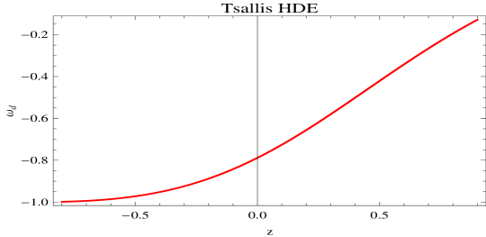
Figure 1: Plot of $\omega_{d}$ versus $z$ for THDE model where $\delta=1.1,\rho_{m0}=1,d^{2}=0.001,B=-1.3,b=0.5.$

The square of the sound speed is given by

$$v_{s}^{2} = \frac{1}{6B(\delta-2)a^{4}H^{3}\dot{H}}\left(9d^{2}\left(d^{2}-1\right)\rho_{m0}a^{3d^{2}}H^{2\delta}\dot{a}-2B(\delta-2)a^{4}H\right.$$ (23)

$$\times \left.\left(3H^{2}\dot{H}-2(\delta-1)\dot{H}^{2}+H\ddot{H}\right)\right).$$

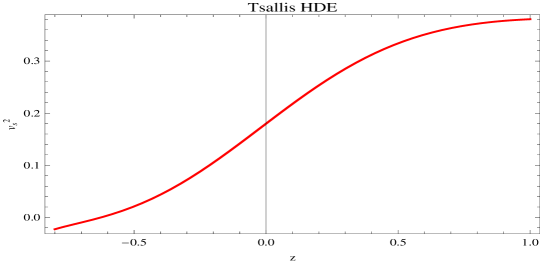
Figure 2: Plot of $v_{s}^{2}$ versus $z$ for THDE model where $\delta=1.1,\rho_{m0}=0.8,d^{2}=0.001,B=-1.3,b=0.5.$

The plot of squared sound speed versus $z$ shown in Figure 2 for different parametric values. This graph is used to analyze the stability of this model. We can see that $v_{s}^{2}>0$, for $-0.6<z<1$ which corresponds to the stability of THDE model. However, model shows instability for $z<-0.6$.

Taking the derivative of the EoS parameter with respect to $\ln a$, we get $\omega^{\prime}_{d}$ as follows:

$$\omega^{\prime}_{d} = \frac{1}{3Ba^{4}H^{6}}\left(-3d^{2}\rho_{m0}^{3d^{2}}H^{2\delta}\left(3\left(d^{2}-1\right)H\dot{a}+(2\delta-4)\dot{H}\right)+2B(\delta-2)\right.$$ (24)

$$\times \left.a^{4}H^{2}\left(-2\dot{H}^{2}+H\ddot{H}\right)\right)$$

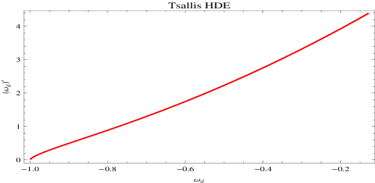
Figure 3: Plot of $\omega_{d}$ versus $\omega_{d}^{\prime}$ for THDE model where $\delta=1.1,\rho_{m0}=1,d^{2}=0.001,B=-1.3,b=0.5.$

The graph of $\omega_{d}$ versus $\omega_{d}^{\prime}$ is shown in Figure 3, for which $\omega_{d}^{\prime}$ depicts positive behavior. Hence, for $\omega_{d}<0$, the evolution parameter shows $\omega_{d}^{\prime}>0$, which represents the thawing region of evolving universe.

4 Rényi Holographic Dark Energy Model

We consider a system with $W$ states with probability of getting $i^{\textmd{th}}$ state $P_{i}$ and satisfies the condition $\Sigma{{}_{i=1}^{W}}P_{i}=1$. Rényi and Tsallis entropies are defined as

$$\mathcal{S}=\frac{1}{\delta}\ln\Sigma{{}_{i=1}^{W}}P{{}_{i}^{1-\delta}},\quad S_{T}=\frac{1}{\delta}\Sigma{{}_{i=1}^{W}}(P{{}_{i}^{1-\delta}}-P_{i}),$$ (25)

where $\delta\equiv 1-U$, where, $U$ is a real parameter. Now, combining above equations we find their mutual relation given as

$$\mathcal{S}=\frac{1}{\delta}\ln(1+\delta S_{T}).$$ (26)

This equation shows that $\mathcal{S}$ belongs to the class of most general entropy functions of homogenous system. Recently, it has been observed that Bekenstine entropy, $S=\frac{A}{4}$ is in fact Tsallis entropy which gives the expression

$$\textsl{S}=\frac{1}{\delta}\ln(1+\delta\frac{A}{4}),$$ (27)

which is the Rényi entropy of the system. Now for the RHDE, we focus on WMAP data for flat universe. Using the assumption $\rho_{d}dv\propto Tds$, we can get RHDE density

$$\rho_{d}=\frac{3C^{2}H^{2}}{8\pi(1+\frac{\delta\pi}{H^{2}})}.$$ (28)

Consider the term $8\pi=1$ substituting in Eq.(28), we get the expression for density as

$$\rho_{d}=\frac{3C^{2}H^{2}}{1+\frac{\delta\pi}{H^{2}}}.$$ (29)

Now, $\frac{dH}{dz}$ is given by

$$\frac{dH}{dz} = \frac{\frac{1}{2}\left(\rho_{m0}(1-d^{2})(1+z)^{3(1-d^{2})}+b^{2}(1+z)^{6}\right)}{\left(1-\frac{2c^{2}H^{2}\left(z^{2}+\delta\pi\right)-c^{2}H^{4}}{\left(H^{2}+\delta\pi\right)^{2}}\right)H(1+z)}$$ (30)

The pressure for this case is obtained as

$$p_{d}=-d^{2}\rho_{m0}a^{-3(1-d^{2})}+\frac{c^{2}H^{2}\left(-3H^{2}\left(\pi\delta+H^{2}\right)-2\left(2\pi\delta+H^{2}\right)\dot{H}\right)}{\left(\pi\delta+H^{2}\right)^{2}}.$$ (31)

The expressions for EoS parameter $\omega_{d}$ can be evaluated from Eq.(12) as follows

$$\omega_{d}=\left(\pi\delta+H^{2}\right)\left(\frac{-d^{2}\rho_{m0}a^{-3(1-d^{2})}}{3c^{2}H^{4}}-\frac{\left(3H^{2}\left(\pi\delta+H^{2}\right)+2\left(2\pi\delta+H^{2}\right)\dot{H}\right)}{3H^{2}\left(\pi\delta+H^{2}\right)^{2}}\right).$$ (32)

Figure 4: Plot of $\omega_{d}$ versus $z$ for RHDE model where $\delta=1.1,\rho_{m0}=0.8,d^{2}=0.001,c=0.1,b=0.05.$

Figure 4 shows the plot of $\omega_{d}$ versus $z$. The trajectory of EoS parameter evolutes the universe from quintessence region towards the $\Lambda$CDM limit. The squared sound speed of this RHDE model is given by using Eq.(13) as

$${v_{s}}^{2} = \frac{3H\left(1-d^{2}\right)d^{2}\rho_{m0}a^{-3(1-d^{2})}\left(\pi\delta+H^{2}\right)^{2}}{6c^{2}H^{3}\left(2\pi\delta+H^{2}\right)\dot{H}}-\frac{1}{3H^{2}\left(2\pi\delta+H^{2}\right)\left(\pi\delta+H^{2}\right)}$$ (33)

$$\times \left\{\dot{H}\left(6\pi^{2}\delta^{2}H^{2}+9\pi\delta H^{4}+3H^{6}+4\pi^{2}\delta^{2}\dot{H}\right)+H\ddot{H}\left(\pi\delta+H^{2}\right)\right.$$

$$\times \left.\left(2\pi\delta+H^{2}\right)\right\}.$$

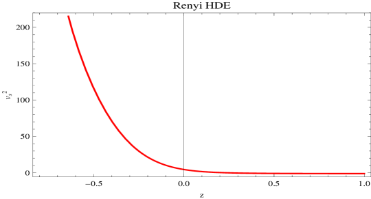
Figure 5: Plot of $v_{s}^{2}$ versus $z$, for RHDE model where $\delta=1.1,\rho_{m0}=0.8,d^{2}=0.001,c=0.1,b=1.5.$

The graph of squared speed of sound is shown in Figure 5 versus $z$. In this case, we have $v_{s}^{2}>0$ for all range of $z$ which shows the stability of RHDE model at the early, present and latter epoch of the universe.

The expression for $\omega^{\prime}_{d}$ is evaluated as:

$$\omega^{\prime}_{d} = \frac{1}{3c^{2}a^{4}H^{6}\left(\pi\delta+H^{2}\right)^{2}}\left\{-d^{2}\rho_{m0}a^{3d^{2}}\left(\pi\delta+H^{2}\right)^{2}\left(3H\dot{a}\left(-1+d^{2}\right)\right.\right.$$ (34)

$$\times \left.\left.\left(\pi\delta+H^{2}\right)-2a\dot{H}\left(2\pi\delta+H^{2}\right)\right)+2c^{2}a^{4}H^{2}\left(4\pi^{2}\delta^{2}+8\pi\delta H^{2}+2H^{4}\right)\dot{H}^{2}\right.$$

$$- \left.2H\left(\pi\delta+H^{2}\right)\left(2\pi\delta+H^{2}\right)\ddot{H}\right\}.$$

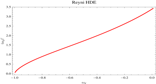
Figure 6: Plot of $\omega_{d}$ versus $\omega_{d}^{\prime}$ for RHDE model where $\delta=1.1,\rho_{m0}=0.8,d^{2}=0.001,c=0.1,b=0.05.$

In Figure (6), we plot the EoS parameter with its evolution parameter to discuss $\omega_{d}-\omega_{d}^{\prime}$ plane for RHDE model. The graph shows that for $\omega_{d}<0$, the evolutionary parameter remains positive at the early, present and latter epoch. This type of behavior depicts the thawing region of the evolving universe.

5 Sharma-Mitall Holographic Dark Energy Model

From the Rényi entropy, we have the generalized entropy content of the system. Using Eq.(26), Sharma-Mittal introduced a two parametric entropy which is defined as

$$S_{SM}=\frac{1}{1-r}\left((\Sigma{{}_{i=1}^{W}}P{{}_{i}^{1-\delta}})^{1-r/\delta}-1\right),$$ (35)

where $r$ is a new free parameter. We can observe that Rényi and Tsallis entropies can be recovered at the proper limits, using Eq.(25) in Eq.(35), we have

$$S_{SM}=\frac{1}{R}((1+\delta S_{T})^{R/\delta}-1),$$ (36)

here, $R\equiv 1-r$. Using the argument that Bekenstine entropy is the proper candidate for Tsallis entropy by using $S=A/4$ where $A$ is horizon entropy, we get the following expression

$$S_{SM}=\frac{1}{R}((1+\delta\frac{A}{4})^{R/\delta}-1),$$ (37)

The relation of UV $(\Lambda)$ cut off, IR (L) cut off and and system horizon (S) is given as

$$\Lambda^{4}\propto\frac{S}{L^{4}}$$ (38)

Now, taking $L\equiv\frac{1}{H}=\sqrt{A/4\pi}$, then the the energy density of DE given by Sharma-Mitall [29] is considered as;

$$\rho_{d}=\frac{3c^{2}H^{4}}{8\pi R}\left[(1+\frac{\delta\pi}{H^{2}})^{R/\delta}-1\right],$$ (39)

here, $c^{2}$ is an unknown free parameter. Using $8\pi=1$ in above equation, we get the following expression for energy density

$$\rho_{d}=\frac{3c^{2}H^{4}}{R}\left[\left(1+\frac{\delta\pi}{H^{2}}\right)^{R/\delta}-1\right].$$ (40)

The differential equation of $H$ is given by

$$\frac{dH}{dz} = \frac{\frac{1}{2}\left(\rho_{m0}(1-d^{2})(1+z)^{3(1-d^{2})}+b^{2}(1+z)^{6}\right)}{1+c^{2}\pi\left(1+\frac{\delta\pi}{H^{2}}\right)^{\frac{R}{\delta}-1}-\frac{2c^{2}H^{2}}{R}\left(\left(1+\frac{\delta\pi}{H^{2}}\right)^{\frac{R}{\delta}}-1\right)H(1+z)}$$ (41)

The pressure can be evaluated by energy conservation Eq.(11) as follows

$$p_{d} = -d^{2}\rho_{m0}a^{-3(1-d^{2})}-c^{2}\left(\frac{3\left(\left(1+\frac{\pi\delta}{H^{2}}\right)^{R/\delta}-1\right)H^{4}}{R}-2\pi\dot{H}\left(1+\frac{\pi\delta}{H^{2}}\right)^{{R/\delta}-1}\right.$$

$$+ \left.\frac{4\left(\left(1+\frac{\pi\delta}{H^{2}}\right)^{R/\delta}-1\right)H^{2}\dot{H}}{R}\right).$$

The EoS parameter for this model is given by

$$\omega_{d} = 2c^{2}\left(\pi\left(1+\frac{\pi\delta}{H^{2}}\right)^{{R/\delta}-1}-\frac{2H^{2}\dot{H}}{R}\left(\left(1+\frac{\pi\delta}{H^{2}}-1\right)^{R/\delta}\right)\right)$$

$$- \frac{d^{2}R\rho_{m0}a^{-3(1-d^{2})}}{3c^{2}H^{4}\left(\left(1+\frac{\delta\pi}{H^{2}}\right)^{{R/\delta}}-1\right)}-1.$$

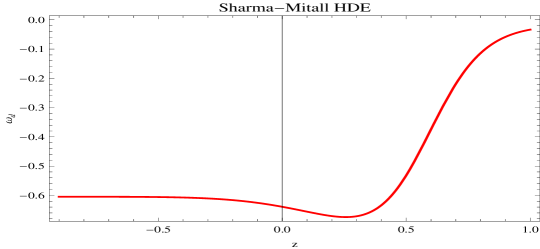
Figure 7: Plot of $\omega_{d}$ versus $z$ for SMHDE where $\delta=1.1,\rho_{m0}=0.01,d^{2}=0.001,c=0.01,b=0.4,R=7.$

The plot of $\omega_{d}$ versus $z$ is shown in Figure 7. The EoS parameter represents the quintessence nature of the universe. The square of the sound speed is evaluated as

$$v_{s}^{2} = \frac{1}{6c^{2}H\dot{H}\left(-\pi\left(1+\frac{\pi\delta}{H^{2}}\right)^{R/\delta-1}+\frac{2H^{2}}{R}\left(\left(1+\frac{\pi\delta}{H^{2}}\right)^{R/\delta}-1\right)\right)}$$ (42)

$$\times \left\{-3d^{2}H\left(-1+d^{2}\right)\rho_{m0}a^{-3(1-d^{2})}+\frac{2c^{2}H}{R}\left(6H^{2}\dot{H}+4\dot{H}^{2}+2H\ddot{H}\right.\right.$$

$$- \left.\left.\frac{1}{\left(\pi\delta+H^{2}\right)^{2}}\left(1+\frac{\pi\delta}{H^{2}}\right)^{R/\delta}\left(3H^{2}\dot{H}\left(\pi\delta+H^{2}\right)\left(-\pi R+2\pi\delta+2H^{2}\right)\right.\right.\right.$$

$$+ \left.\left.\left.2\dot{H}\left(\pi^{2}(R-2\delta)(R-\delta)-2\dot{H}^{2}\pi(R-2\delta)H^{2}+2H^{4}\right)\right)+H\dot{H}\left(\pi\delta+H^{2}\right)\right.\right.$$

$$\times \left.\left.\left(-\pi R+2\pi\delta+2H^{2}\right)\ddot{H}\right)\right\}.$$

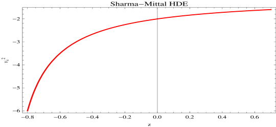
Figure 8: Plot of $v_{s}^{2}$ versus $z$ for SMHDE where $\delta=1.1,\rho_{m0}=0.8,d^{2}=0.001,c=0.8,b=0.05,R=7.$

In Figure 8, we draw $v_{s}^{2}$ versus $z$ which shows the un-stable behavior of the SMHDE model as $v_{s}^{2}<0$ at early, present and latter epoch.

$$\omega^{\prime}_{d} = -\frac{1}{3\left(\left(1+\frac{\pi\delta}{H^{2}}\right)^{R/\delta}-1\right)^{2}H^{6}}\left(\frac{1}{\left(\pi\delta+H^{2}\right)^{2}}2H^{2}\left(2\left(-2\left(\pi\delta+H^{2}\right)^{2}\right.\right.\right.$$

$$+ \left.\left.\left.\left(1+\frac{\pi\delta}{H^{2}}\right)^{2R/\delta}\left(\pi^{2}(R-2\delta)\delta+2\pi(R-2\delta)H^{2}-2H^{4}\right)+\left(1+\frac{\pi\delta}{H^{2}}\right)^{R/\delta}\right.\right.\right.$$

$$\times \left.\left.\left.\left(-\pi^{2}\left(R^{2}+R\delta-4\delta^{2}\right)-2\pi(R-4\delta)H^{2}+4H^{4}\right)\right)\dot{H}^{2}+\left(\pi\delta+H^{2}\right)\right.\right.$$

$$\times \left.\left.\left(\left(1+\frac{\pi\delta}{H^{2}}\right)^{R/\delta}-1\right)H\left(-2\left(\pi\delta+H^{2}\right)+\left(1+\frac{\pi\delta}{H^{2}}\right)^{R/\delta}\right.\right.\right.$$

$$\times \left.\left.\left.\left(-\pi R+2\pi\delta+2H^{2}\right)\right)\ddot{H}\right)+\frac{3d^{2}\left(-1+d^{2}\right)}{c^{2}}\rho_{m0}Ra^{-3(1-d^{2})}H^{2}\right.$$

$$\times \left.\left(\left(1+\frac{\pi\delta}{H^{2}}\right)^{R/\delta}-1\right)+\frac{2d^{2}\rho_{m0}Ra^{-3(1-d^{2})}}{c^{2}\left(\pi\delta+H^{2}\right)}\left(\left(\pi(R-2\delta)-2H^{2}\right)\right.\right.$$

$$\times \left.\left.\left(1+\frac{\pi\delta}{H^{2}}\right)^{R/\delta}+2\left(\pi\delta+H^{2}\right)\right)\dot{H}\right)$$

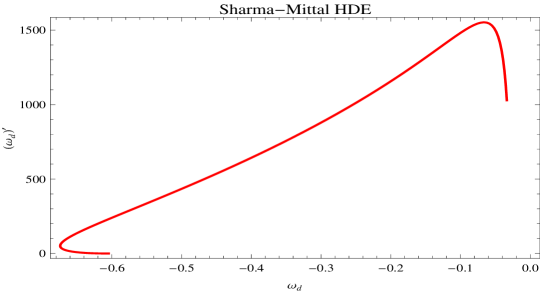
Figure 9: Plot of $\omega_{d}$ versus $\omega_{d}^{\prime}$ for different values of $\delta$ for SMHDE where $\delta=1.1,\rho_{m0}=0.01,d^{2}=0.001,c=0.01,b=0.4,R=7.$

Figure 9 shows the plot of $\omega_{d}$-$\omega_{d}^{\prime}$ plane to classify the dynamical region for the given model. We can see that, $\omega_{d}^{\prime}>0$ for $\omega_{d}<0$, which indicates the thawing region of the universe.

6 Conclusion

In this paper, we have discussed the THDE, RHDE and SMHDE models in the frame work of Chern-Simons modified theory of gravity. We have taken the flat FRW universe and linear interaction term is chosen for the interacting scenario between DE and dark matter. We have evaluated the different cosmological parameters (equation of state parameter and squared sound speed), $\omega_{d}-\omega_{d}^{\prime}$ cosmological plane. The trajectories of all these models have been plotted with different constant parametric values.

We have summarized our results in the following table.
Table 1: Summary of the cosmological parameters and plane.

DE models	$\omega_{d}$	$v^{2}_{s}$	$\omega_{d}-\omega_{d}^{\prime}$
THDE	quintessence-to-vacuum	partially stability	thawing region
RHDE	quintessence-to-vacuum	stability	thawing region
SMHDE	quintessence	un-stable	thawing region

Jawad et al. [32] have explored various cosmological parameters (equation of state, squared speed of sound, Om-diagnostic) and cosmological planes in the framework of dynamical Chern-Simons modified gravity with the new holographic dark energy model. They observed that the equation of state parameter gives consistent ranges by using different observational schemes. They also found that the squared speed of sound shows a stable solution. They suggested that the results of cosmological parameters show consistency with recent observational data. Jawad et al. [33] have also considered the power law and the entropy corrected HDE models with Hubble horizon in the dynamical Chern Simons modified gravity. They have also explored various cosmological parameters and planes and found consistent results with observational data. Nadeem et al. [34] have also investigated the interacting modified QCD ghost DE and generalized ghost pilgrim DE with cold dark matter in the framework of dynamical Chern-Simons modified gravity. It is found that the results of cosmological parameters as well as planes explain the accelerated expansion of the Universe and are compatible with observational data.

However, the present work is different from the above mentioned works in which we have taken recently proposed DE models along with non-linear interaction term and found interesting and compatible results regarding current accelerated expansion of the universe.

Data Availability

The data used to support the findings of this study are available from the corresponding author upon request.

References

- [1] A. G. Riess et al.: Astron. J. 116 (1998) 1009.
- [2] S. Perlmutter et al.: Astrophys. J. 517 (1999) 565.
- [3] P. deBernardis et al.: Nature 404 (2000) 955.
- [4] S. Perlmutter et al.: Astrophys. J. 598 (2003) 102.
- [5] M. Colless et al.: Mon. Not. R. Astron. Soc. 328 (2001) 1039.
- [6] M. Tegmark et al.: Phys. Rev. D 69 (2004) 103501.
- [7] S. Cole et al.: Mon. Not. R. Astron. Soc. 362 (2005) 505.
- [8] V. Springel, C. S. Frenk and S. M. D. White.: Nature 440 (2006) 1137.
- [9] S. Hanany et al.: Astrophys. J. Lett. 545 (2000) L5.
- [10] C. B. Netterfield et al.: Astrophys. J. 571 (2002) 604.
- [11] D. N. Spergel et al.: Astrophys. J. Suppl. 148 (2003) 175.
- [12] Chiba, T., Okabe, T. and Yamaguchi, M.: Phys. Rev. D 62 (2000) 023511.
- [13] Setare, M.R.: Eur. Phys. J. C 52 (2007) 689.
- [14] Bernardini, A.E. and Bertolami, O.: Phys. Rev. D 77 (2008) 083506.
- [15] Hsu, S.D.H.: Phys. Lett. B 594 (2004) 13.
- [16] Li, M.: Phys. Lett. B 603 (2004) 1.
- [17] Bamba, K. et al.: Astrophys. Space Sci. 342 (2012) 155.
- [18] Turner, M.S.: Int. J. Mod. Phys. A 17 (2002) 180.
- [19] E. H. Baffou, A. V. Kpadonou, M. E. Rodrigues, M. J. S. Houndjo and J. Tossa.: Astrophys. Space Sci 355 (2014) 2197.
- [20] S. Nojiri and S.D. Odintsov.: Phys. Lett. B 631 (2005) 1.
- [21] M. Roos.: Introduction to Cosmology (John Wiley and Sons, UK, 2003)
- [22] S. Nojiri and S. D. Odintsov.: Phys. Lett. B 639 (2006) 144.
- [23] K. Bamba, S. Capozziello, S. Nojiri and S. D. Odintsov.: Astrophys. Space Sci. 342 (2012) 155.
- [24] A. G. Cohen et. al, Phys. Rev. Lett. 73 (1999) 4971.
- [25] A. Pasqua, R. da Rochab, S. Chattopadhyay: Eur. Phys. J. C 75, 44 (2015).
-
[26]
H. Moradpour, A. Sheykhi, C. Corda, I. G. Salako, Phys. Lett. B 783 (2018) 82;
H. Moradpour, A. Bonilla, E.M.C. Abreu, J.A. Neto, Phys. Rev. D, 96 (2017) 123504;
H. Moradpour, Int. J. Theor. Phys., 55 (2016) 4176;
- [27] M. Tavayef, A. Sheykhi, K. Bamba and H. Moradpour.: Phys. Lett. B 781 (2018) 195.
- [28] H. Moradpour et al.: arXiv:1803.02195.
- [29] A. Sayahian Jahromi et al.: Phys. Lett. B, 780 (2018) 21-24.
- [30] E. J. Copeland, M. Sami and S. Tsujikawa: Int. J. Mod. Phys. D 15 (2006) 1753.
- [31] C. Tsallis, L. J. L. Citro.: Eur. Phys. J. C 73 (2013) 2487.
- [32] A. Jawad, S. Rani, and T. Nawaz: Eur. Phys. J. Plus 131 (2016) 282.
- [33] A. Jawad, S. Rani, and N. Azhar: Int. J. Mod. Phys. D 26 (2016) 1750040.
- [34] N. Azhar et al.: Int. J. Geom. Meth. Mod. Phys. 15 (2018) 1850034.