Analysis of Divide & Conquer strategies for the
0-1 Minimization Knapsack Problem

Abstract

We introduce and asses several Divide & Conquer heuristic strategies aimed to solve large instances of the 0̧-1 Minimization Knapsack Problem. The method subdivides a large problem in two smaller ones (or recursive iterations of the same principle), to lower down the global computational complexity of the original problem, at the expense of a moderate loss of quality in the solution. Theoretical mathematical results are presented in order to guarantee an algorithmically successful application of the method and to suggest the potential strategies for its implementation. In contrast, due to the lack of theoretical results, the solution’s quality deterioration is measured empirically by means of Monte Carlo simulations for several types and values of the chosen strategies. Finally, introducing parameters of efficiency we suggest the best strategies depending on the data input.

1 Introduction

The Knapsack Problem (KP) is, beyond dispute, one of the fundamental problems in integer optimization for three main reasons. First, due to its simplicity with respect to a general linear integer (or mixed integer) optimization problem. Second, because of its occurrence as a subproblem of an overwhelming number of optimization problems, including a wide variety of real life situations which can be modeled by KP. Third, because it belongs to the NP hard class problems which makes it relevant from the theoretical perspective. As a natural consequence, there is a vast literature dedicated to the KP solution, comprising a broad spectrum between exact algorithms such as Dynamic Programming (DP) and Branch & Bound (B&B) techniques [11], metaheuristic schemes such as Genetic Algorithms (GA), Ant Colony Algorithms (ACO’s) and hybrid algorithms, including matheuristics and symheuristics [3], [4], [10], [16], [18]; an early review of non-standard versions of KP is found in [12], a detailed review of some versions is found in the texts [11] and [14]. The convergence analysis for some of the aforementioned algorithms is presented in [5], [7], [8], [9]. As with any optimization problem, for the KP solution it is crucial to exploit the trade-off between the quality of the solution in terms of the value of the objective function, and the computational effort required to obtain it.

Both, exact methods and metaheuristic algorithms have disadvantages. Exact algorithms such as DP and B&B usually are insufficient to address large instances: all dynamic programming versions for KP are pseudo-polynomial, i.e. time and memory requirements are dependent on the instance size. Commonly, the computational complexity of the algorithms B&B cannot be explicitly described, as it is not possible to estimate a priori the number of search tree nodes required (see [11], [15]). On the other hand, most metaheuristics lack sufficient theoretical justification. Despite the widespread success of such techniques, among researchers there is little understanding about the key aspects of their design, including the identification of search space characteristics that influence the difficulty of the problem. There are some theoretical results related to the convergence of algorithms under appropriate probabilistic hypotheses, however these are not useful from the practical point of view. Moreover, it is not possible to argue that any of the particular metaheuristics is on average superior to any other, so the choice of a metaheuristics to address a specific optimization problem depends largely on the user’s experience [16].

As a consequence of the KP’s relevance, it is natural that any proposed method for solving integer optimization problems: theoretical, empirical or mixed, is usually first tested on a Knapsack Problem. This is the case of the present work, where we introduce a Divide and Conquer (D&C) strategy aimed to solve large instances of the 0-1 Minimization Knapsack Problem 1 below (from now on 0-1 MKP). The main goal of the proposed approach is to reduce the computational complexity of the 0-1 MKP by subdividing the original/initial problem in two smaller subproblems, at the price of giving up (to some extent) quality of the solution. Moreover, using multiple recursive D&C iterations the initial problem can be decomposed on several subproblems of suitable size (at the price of further deterioration in the solution’s quality), in a multilevel scheme, see Figures 1, 2 and 3. The multilevel paradigm is not a metaheuristic in itself, on the contrary, it must act in collaboration with some solution strategy, be it an exact or approximate procedure. For the method to be worthy, the loss of quality vs. the reduction of computational time must lie within an acceptable range. Consequently, the present work first introduces the technique, together with several strategies for its implementation. Next, the quality is defined using several parameters of efficiency. Finally, since no theoretical results can be mathematically shown for measuring the efficiency of the method, we proceed empirically using Monte Carlo simulations and the Law of Large Numbers (see Theorem 7 below) to identify which strategy will likely be the best, when the data input of the problem are regarded as random variables with known probabilistic distribution.

We close this section mentioning that different authors have reported the increased performance of metaheuristic techniques when used in conjunction with a multilevel scheme on large instances. The multilevel paradigm has been used mainly in mesh construction, Graph Partition Problem (GPP), Capacitated Multicommodity Network Design (CMND), Covering Design (CD), Graph Colouring (GC), Graph Ordering (GO), Traveling Salesman Problem (TSP) and Vehicle Routing Problem (VRP) [1], [17]. To the Authors’ best knowledge, the use of a multilevel D&C scheme for solving the 0-1 Minimization Knapsack Problem has not been reported.

2 Preliminaries

In this section the general setting and preliminaries of the problem are presented. We start introducing the mathematical notation. For any natural number $N\in\bm{\mathbbm{N}}$, the symbol $[N]\overset{\mathbf{def}}{=}\{1,2,\ldots,N\}$ indicates the set/window of the first $N$ natural numbers. For any set $E$ we denote by $|E|$ its cardinal and $\wp(E)$ its power set. A particularly important set is $\mathcal{S}_{N}$, where $\mathcal{S}_{N}$ denotes the collection of all permutations in $[N]$, its elements will be usually denoted by $\pi,\sigma,\tau$, etc. Random variables will be represented with upright capital letters, e.g. $\mathsf{X},\mathsf{Y},\mathsf{Z},...$ and its respective expectations with $\bm{\mathbb{E}}(\mathsf{X}),\bm{\mathbb{E}}(\mathsf{Y}),\bm{\mathbb{E}}(\mathsf{Z}),...$. Vectors are indicated with bold letters, namely $\bm{p},\bm{g},...$ etc. Particularly important collections of objects will be written with calligraphic characters, e.g. $\mathcal{A},\mathcal{D},\mathcal{E}$ to add emphasis. For any real number $x\in\bm{\mathbbm{R}}$ the floor and ceiling function are given (and denoted) by $\lfloor x\rfloor\overset{\mathbf{def}}{=}\max\{k:\ell\leq x,\,k\text{ integer}\}$, $\lceil x\rceil\overset{\mathbf{def}}{=}\max\{k:k\geq x,\,k\text{ integer}\}$, respectively.

2.1 The Problem

Now we introduce the 0-1 Minimization Knapsack Problem.

Problem 1 (0-1 Minimization KP).

$$\min\sum\limits_{i\,\in\,[N]}p_{i}x_{i},$$ (1a)

subject to

$$\sum\limits_{i\,\in\,[N]}c_{i}x_{i}\geq D,$$ (1b)

$$x_{i}\in\{0,1\}, \text{for all }i\,\in\,[N].$$ (1c)

Here, $\bm{x}\overset{\mathbf{def}}{=}\big{(}x_{i}:i\in[N]\big{)}$ is the list of binary valued decision variables. In addition, the capacity coefficients $\bm{c}\overset{\mathbf{def}}{=}\big{(}c_{i}:i\in[N]\big{)}$ as well as the costs $\bm{p}\overset{\mathbf{def}}{=}\big{(}p_{i}:i\in[N]\big{)}$, are all positive integers. In the sequel, the feasible set is denoted by

$$S\overset{\mathbf{def}}{=}\big{\{}\bm{x}\in\{0,1\}^{N}:\bm{c}\cdot\bm{x}\geq D\big{\}}$$ (2)

and the problem can be written concisely as

$$z^{*}\overset{\mathbf{def}}{=}\min\big{\{}\bm{p}\cdot\bm{x}:\bm{x}\,\in\,S\big{\}},$$ (3)

where $z_{*}$ denotes the optimal solution value.

In general, the 0-1 MKP can be understood as the problem of buying items (buses, aircraft, ships fleet), denoted by the index $i=1,\ldots,N$, with corresponding costs $p_{i}$ and capacities $c_{i}$. Therefore, the natural question is to choose a set of items to minimize its total cost but whose overall capacity satisfies a minimum threshold demand $D$. Observe that the solution of Problem 1 above can be found using the solution of the following Knapsack Problem

Problem 2.

$$\max\sum\limits_{i\,\in\,[N]}p_{i}\xi_{i},$$ (4a)

subject to

$$\sum\limits_{i\,\in\,[N]}c_{i}\xi_{i}\leq\sum\limits_{i\,\in\,[N]}c_{i}-D,$$ (4b)

$$\xi_{i}\in\{0,1\}, \text{for all }i\,\in\,[N].$$ (4c)

Proposition 1.

Let $\bm{\xi}=\big{(}\xi_{i}:i\in[N]\big{)}\in\{0,1\}^{N}$ be a solution to Problem 2 and define $x_{i}\overset{\mathbf{def}}{=}1-\xi_{i}$ for all $i\in[N]$ then, the vector $\bm{x}=\big{(}x_{i}:i\in[N]\big{)}\in\{0,1\}^{N}$ is a solution to Problem 1.

Proof.

The proof uses the well-known classic transformation of complementary binary variables, $x_{i}=1-\xi_{i}\in\{0,1\}$ for all $i\in[N]$, to relate the problems 1 and 2 (see Section 13.3.3 in [11] for details). ∎∎

2.2 Greedy Algorithm vs Linear Optimization Relaxation

In this section, we explore the relationship between the solution of the natural linear relaxation of Problem 1 and the solution provided by the natural Greedy Algorithm. First we introduce the following definitions

Definition 1.

Let $\bm{c}=\big{(}c_{i}:i\in[N]\big{)}$, $\bm{p}=\big{(}p_{i}:i\in[N]\big{)}$ be the lists of capacities and prices respectively, we define the list of specific weights by

$$\gamma_{i}\overset{\mathbf{def}}{=}\frac{c_{i}}{p_{i}}\,, \text{for all }i\in[N].$$ (5)

Consider now the Greedy Algorithm 1 to find a feasible solution to Problem 1.

Algorithm 1 Greedy Algorithm, returns feasible solution to Problem 1 $\big{(}y_{i}:i\in[N]\big{)}$ and corresponding value of objective function $\sum\big{\{}p_{i}y_{i}:i\,\in\,[N]\big{\}}$

1:procedure Greedy Algorithm(Prices: $\bm{p}=\big{(}p_{i}:i\in[N]\big{)}$, Capacities: $\bm{c}=\big{(}c_{i}:i\in[N]\big{)}$, Demand: $D$)

2:     if $\sum\limits_{i\,\in\,[N]}c_{i}<D$ then print “Feasible region is empty” $\triangleright$ Checking if the problem is infeasible

3:     else

4:         compute list of specific weights $\big{(}\gamma_{i}:i\in[N]\big{)}$ $\triangleright$ Introduced in Definition 1.

5:         sort the list $\big{(}\gamma_{i}:i\in[N]\big{)}$ in descending order

6:         denote by $\sigma\in\mathcal{S}[N]$ the associated ordering permutation, i.e.,

$$\gamma_{\sigma(i)}\geq\gamma_{\sigma(i+1)}, \text{for all }i\in[N-1].$$ (6)

7:         $y_{i}=0$ for all $i\in[N]$, $capacity=0$ $\triangleright$ Initializing feasible solution and capacity

8:         i = 1

9:         while $capacity\geq D$ do $y_{\sigma(i)}=1$,   $capacity=capacity+c_{\sigma(i)}$,  $i=i+1$ 

10:         end while

11:         return $\big{(}y_{i}:i\in[N]\big{)}$, $\sum\limits_{i\,\in\,[N]}p_{i}y_{i}$ $\triangleright$ Feasible solution and corresponding value of objective function

12:     end if

13:end procedure

Observe that due to the condition ($\sum\limits_{i\,\in\,[N]}c_{i}\geq D$) for the loop to start, it will stop after a finite number of iterations. Next we introduce

Definition 2.

The natural linear relaxation of Problem 1, is given by

Problem 3 (Linear Relaxation, 0-1 Minimization KP).

$$\min\sum\limits_{i\,\in\,[N]}p_{i}\xi_{i},$$ (7a)

subject to

$$\sum\limits_{i\,\in\,[N]}c_{i}\xi_{i}\geq D,$$ (7b)

$$0\leq\xi_{i}\leq 1, \text{for all }i\,\in\,[N],$$ (7c)

i.e., the decision variables $\big{(}\xi_{i}:i\in[N]\big{)}$ are are now real-valued.

Next we introduce a convenient notation and recall a classic result

Definition 3.

Let $\bm{\xi}=\big{(}\xi_{i}:i\in[N]\big{)}$ be a solution of Problem 3 define the index sets

$$P\overset{\mathbf{def}}{=}\big{\{}i\in[N]:\xi_{i}>0\big{\}}, Z\overset{\mathbf{def}}{=}\big{\{}i\in[N]:\xi_{i}=0\big{\}}.$$ (8)

Define its associated integer solution $\bm{x}^{\bm{\xi}}=\big{(}x_{i}^{\bm{\xi}}:i\in[N]\big{)}$ by

$$x_{i}^{\bm{\xi}}\overset{\mathbf{def}}{=}\begin{cases}1&i\in P,\\ 0&i\in Z.\end{cases}$$ (9)

Theorem 2.

Let $\bm{\xi}=\big{(}\xi_{i}:i\in[N]\big{)}$ be an optimal solution of Problem 3 and let $\bm{x}^{\bm{\xi}}$ be as in Definition 3 above. Then, $\bm{x}^{\bm{\xi}}=\big{(}x_{i}^{\bm{\xi}}:i\in[N]\big{)}$ is the solution furnished by the Greedy Algorithm 1.

Proof.

See Theorem 2.1 in [11]. ∎∎

Remark 1.

It is important to stress that the Greedy Algorithm 1 may not produce an optimal solution as the following example shows. Consider Problem 1 for $D=40$ and the following data.

Item	Capacity: $\bm{c}$	Price: $\bm{p}$	Specific Weigh: $\bm{\gamma}$
1	100	4	25
2	40	2	20

Table 1: Remark 1 Data

Clearly, the Greedy Algorithm 1 would choose the solution $\bm{x}=\big{(}1,0\big{)}$ with $\bm{p}\cdot\bm{x}=4$ while $\bm{y}=\big{(}0,1\big{)}$ gives $\bm{p}\cdot\bm{y}=2$ and $\bm{x}$ is not optimal. Moreover, the linear relaxation of this problem would yield $\bm{\xi}=\big{(}0.4,0\big{)}$ with $\bm{p}\cdot\bm{\xi}=1.6$ and associated integer solution $\bm{x}^{\bm{\xi}}=\big{(}1,0\big{)}$ i.e, the solution produced by the Greedy Algorithm 1.

2.3 Introducing a Price-Capacity Rate

In the sequel we adopt a relationship between capacities $\bm{c}$ and prices $\bm{p}$ as it usually holds in real life scenarios.

Definition 4 (Rate Price Capacity).

Let $r\in\big{[}1,\max\limits_{i}c_{i}\big{]}$ be a fixed price-capacity increase threshold, then

$$p_{i}\overset{\mathbf{def}}{=}\Big{\lceil}\frac{c_{i}}{r}\Big{\rceil}, \text{for all }i\in[N].$$ (10)

In the following, we refer to $r$ as the price-capacity rate.

Next we recall the main result of this part

Theorem 3.

Let $\big{(}c_{i}:i\in[N]\big{)}$ be a given list of capacities, let the list of prices $\big{(}p_{i}:i\in[N]\big{)}$ be computed by the map (10) and let $r$ be the price-capacity rate introduced in Definition 4.

1. The Greedy Algorithm 1 produces the exact solution for $r\geq\max\limits_{i}c_{i}$.

2. Let $r|c_{i}$ for all $i\in[N]$ (i.e, a common divisor of all the capacities). Then, the effectiveness of the Greedy Algorithm 1 is entirely random.

3. Let $r|c_{i}$ for all $i\in[N]$ (i.e, a common divisor of all the capacities). Let $\bm{\xi}=\big{(}\xi_{i}:i\in[N]\big{)}$ be an optimal solution of Problem 3 furnished by the Simplex Algorithm and let $\bm{x}^{\bm{\xi}}$ be as in Definition 3. Then, $\bm{x}^{\bm{\xi}}$ is a random element of the set

   $$K\overset{\mathbf{def}}{=}\Big{\{}\bm{x}\in S:\sum\limits_{i\,\in\,A}c_{i}x_{i}<D,\;\forall\,A\subsetneq\{i\in[N]:x_{i}=1\}\Big{\}},$$ (11)

   where, $S$ is the set of feasible solutions to Problem1, introduced in Expression (2).

Proof.

See [11]. ∎∎

Remark 2.

1. Observe that if $r|c_{i}$ for all $i\in[N]$, the Problem (1) becomes

   $$\min\frac{1}{r}\sum\limits_{i\,\in\,[N]}c_{i}x_{i}, S=\Big{\{}\bm{x}\in\{0,1\}^{N}:\sum\limits_{i\,\in\,[N]}c_{i}x_{i}\geq D\Big{\}}.$$

   Hence, it reduces to a problem of approximating and integer from above using an integer partition of $\sum\limits_{i}c_{i}$ in $N$ blocks.

2. Notice that if $r=\dfrac{d}{q}$ with $d$ a common divisor of the capacities, the conclusion of Theorem 3 part (ii) holds.

3. Given that the Greedy Algorithm effectiveness becomes entirely random when $r$ is a common divisor of the capacities, we would like to use another criterion to distinguish the eligible items. To this end, the only possibility is to sort them according to its capacities. However, using the capacity as Greed function may not produce the exact solution as the Greedy Algorithm produced for the case $r\geq\max\limits_{i}c_{i}$. Consider the following example

   Item	Capacity	$D=11$		$D=15$
   	$\bm{c}$	Greedy Decreasing	Optimal	Greedy Increasing	Optimal
   1	10	1	0	0	0
   2	9	1	0	0	0
   3	8	0	0	1	1
   4	7	0	1	1	1
   5	6	0	1	1	0

   Table 2: Remark 2 Data

3 A Divide & Conquer Approach

In the present section we introduce the Divide and Conquer method together with some theoretical results to assure the successful implementation of the method, from the algorithmic point of view. We begin with the following definition

Definition 5 (Divide & Conquer pairs and trees).

1. Let $\bm{c}=\big{(}c_{i}:i\in[N]\big{)}$ and $\bm{p}=\big{(}p_{i}:i\in[N]\big{)}$ be the data associated to Problem 1. A subproblem of Problem 1 is an integer problem with the following structure

   $$\min\sum\limits_{i\,\in\,A}p_{i}x_{i}, A\subseteq[N],$$

   subject to

   $$\sum\limits_{i\,\in\,A}c_{i}x_{i}\geq D^{A}, D^{A}\leq D,$$

   $$x_{i}\in\{0,1\}, \text{for all }i\,\in\,A.$$

2. Let $(A^{0},A^{1})$ be a set partition of $[N]$ and let $(D^{0},D^{1})$ be an integer partition of $D$ i.e., $D=D^{0}+D^{1}$. We say a Divide and Conquer instance of Problem 1 is the pair of subproblems $\big{(}\Pi^{b}:\,b\in\{0,1\}\big{)}$, defined by

   Problem 4 ($\Pi^{b},b=0,1$).

   $$\min\sum\limits_{i\,\in\,A^{b}}p_{i}x_{i},$$ (12a)

   subject to

   $$\sum\limits_{i\,\in\,A^{b}}c_{i}x_{i}\geq D^{b},$$ (12b)

   $$x_{i}\in\{0,1\}, \text{for all }i\,\in\,A^{b}.$$ (12c)

   In the sequel, we refer to $\big{(}\Pi^{b},b=0,1\big{)}$ as a D&C pair. Defining

   $$c^{b}_{i}\overset{\mathbf{def}}{=}\begin{cases}c_{i}&i\in A^{b},\\ 0&i\notin A^{b},\end{cases} p^{b}_{i}\overset{\mathbf{def}}{=}\begin{cases}p_{i}&i\in A^{b},\\ 0&i\notin A^{b},\end{cases}$$

   the corresponding feasible sets and the D&C pair can be respectively written

   $$z^{b}_{*}\overset{\mathbf{def}}{=}\min\big{\{}\bm{p}^{b}\cdot\bm{y}:\bm{y}\in S^{b}\} S^{b}\overset{\mathbf{def}}{=}\big{\{}\bm{y}\in\{0,1\}^{N}:\bm{c}^{b}\cdot\bm{y}\geq D^{b}\big{\}},$$ with (13)

   where $z^{b}_{*}$ denotes the optimal solution value of the problem $\Pi^{b}$.

3. A D&C tree (see Figures 1, 2 and 3 below) for Problem 1 is a binary tree satisfying the following

   1. Every vertex of the tree is in bijective correspondence with a subproblem of Problem 1.

   2. The root of the tree is associated with Problem 1 itself.

   3. Every internal vertex $V$ (which is not a leave) has a left and right children, $V_{l},V_{r}$ respectively, whose associated subproblems make a D&C pair for the subproblem associated to $V$.

Remark 3.

1. Observe that, due to property (iii) a D&C tree is, in particular, a complete binary tree (see [6] pg 127).

2. In the same way that in the knapsack problem the eligible items are identified with their corresponding labels $j=1,\ldots,N$, from now on, in order to ease notation, we identify every vertex of a D&C tree with its associated subproblem. More specifically, a vertex/node of a D&C tree will also act as the label of a subproblem of Problem 1. Given that the vertex-subproblem assignment is a bijective map, such identification will introduce no confusion, see Figure 1-Table 5 and Figure 2-Table 6 for concrete examples; see also Figure 3 below.

Theorem 4.

Suppose that Problem 1 is feasible, then

1. A feasible solution $\bm{y}$ of Problem 1 can be infeasible for at most one problem of the D&C pair.

2. At most one problem of the D&C pair is infeasible.

3. Let $\big{(}A^{b}:b\in\{0,1\}\big{)}$ be a fixed partition of $[N]$ then, both Problems 4, $\big{(}\Pi^{b}:b\in\{0,1\}\big{)}$ are feasible if and only if

   $$D-\sum\limits_{i\,\in\,A^{1-b}}c_{i}\leq D^{b}\leq\sum\limits_{i\,\in\,A^{b}}c_{i}, \text{for }b=0,1.$$ (14)

4. Let $\big{(}A^{b}:b\in\{0,1\}\big{)}$ be a fixed partition of $[N]$ and define

   $$D^{0}\overset{\mathbf{def}}{=}\bigg{\lfloor}\frac{D}{\sum\{c_{i}:i\in[N]\}}\sum\limits_{i\,\in\,A^{0}}c_{i}\bigg{\rfloor}, D^{1}\overset{\mathbf{def}}{=}D-D^{0}.$$ (15)

   Then, if

   $$\frac{D}{\sum\{c_{i}:i\in[N]\}}\,\sum\limits_{i\,\in\,A^{1}}c_{i}+1\leq\sum\limits_{i\,\in\,A^{1}}c_{i}\,,$$ (16)

   both Problems 4, $\big{(}\Pi^{b}:b\in\{0,1\}\big{)}$ are feasible.

5. The following inclusions for the feasible sets $S^{0},S^{1},S$ hold

   $$S\subseteq S^{0}\cup S^{1}, S^{0}\cap S^{1}\subseteq S.$$ (17)

Proof.

1. Let $\bm{y}$ be a feasible solution of Problem 1, then $\sum\limits_{i\,\in\,[N]}c_{i}y_{i}\geq D$; equivalently

   $$\sum_{b\,\in\,\{0,1\}}\sum\limits_{i\,\in\,A^{b}}c_{i}y_{i}\geq D^{0}+D^{1}.$$

   Hence, if $\bm{y}$ is $\Pi^{b}$-infeasible we have $\sum\limits_{i\,\in\,A^{b}}c_{i}y_{i}<D^{b}$ and the expression above writes

   $$\sum\limits_{i\,\in\,A^{1-b}}c_{i}y_{i}\geq D^{1-b}+D^{b}-\sum\limits_{i\,\in\,A^{b}}c_{i}y_{i}>D^{1-b},$$

   i.e., $\bm{y}$ is $\Pi^{1-b}$-feasible. Since $b\in\{0,1\}$ was arbitrary, the claim of this part follows.

2. Since Problem 1 is feasible, the vector $\bm{y}\in\{0,1\}^{N}$ having all its entries equal to one is also feasible, due to the previous part the result follows.

3. Fix $b\in\{0,1\}$ arbitrary, then it is trivial to see that the second inequality in (14) is necessary and sufficient condition for the problem $\Pi^{b}$ to be feasible, as well as the condition $D^{1-b}\leq\sum\limits_{i\,\in\,A^{1-b}}c_{i}$ is necessary and sufficient for $\Pi^{1-b}$ to be feasible. Recalling that $D^{b}=D-D^{1-b}$, the first inequality in (14) follows.

4. Since Problem 1 is feasible then $D\leq\sum\{c_{i}:i\in[N]\}$, therefore

   $$D^{0}=\bigg{\lfloor}\frac{D}{\sum\{c_{i}:i\in[N]\}}\sum\limits_{i\,\in\,A^{0}}c_{i}\bigg{\rfloor}\leq\bigg{\lfloor}\sum\limits_{i\,\in\,A^{0}}c_{i}\bigg{\rfloor}=\sum\limits_{i\,\in\,A^{0}}c_{i},$$

   i.e., the problem $\Pi^{0}$ is feasible. On the other hand,

   $$D^{0}=\bigg{\lfloor}\frac{D}{\sum\{c_{i}:i\in[N]\}}\sum\limits_{i\,\in\,A^{0}}c_{i}\bigg{\rfloor}\geq\frac{D}{\sum\{c_{i}:i\in[N]\}}\sum\limits_{i\,\in\,A^{0}}c_{i}-1.$$

   Since $D^{1}=D-D^{0}$, we have

   $$D^{1} \leq D-\frac{D}{\sum\{c_{i}:i\in[N]\}}\sum\limits_{i\,\in\,A^{0}}c_{i}+1$$

   $$=\frac{D}{\sum\{c_{i}:i\in[N]\}}\sum\limits_{i\,\in\,A^{1}}c_{i}+1$$

   $$\leq\sum\limits_{i\,\in\,A^{1}}c_{i},$$

   where the last bound holds due to Inequality 16. Hence, the problem $\Pi^{1}$ is also feasible.

5. Due to the first part, if $\bm{y}\in S$ then it must be $\Pi^{0}$ or $\Pi^{1}$-feasible. Equivalently, it belongs to $S^{0}$ or $S^{1}$, i.e. $\bm{y}\in S^{0}\cup S^{1}$.

   Finally, if $\bm{y}\in S^{0}\cap S^{1}$ then $\sum\limits_{i\,\in\,A^{b}}c_{i}y_{i}\geq D^{b}$ for $b=0,1$. Adding both inequalities yields

   $$\bm{c}\cdot\bm{y}=\sum\limits_{i\,\in\,[N]}c_{i}y_{i}=\sum\limits_{i\,\in\,A^{0}}c_{i}y_{i}+\sum\limits_{i\,\in\,A^{1}}c_{i}y_{i}\geq D^{0}+D^{1}=D,$$

   i.e., $y$ belongs to the set $S$ and the proof is complete. ∎

∎

Remark 4.

Observe that Inequality 16 in (iv) from Theorem 4, is a mild hypothesis. It is equivalent to

$$D\leq\frac{\sum\{c_{i}:i\,\in\,A^{1}\}-1}{\sum\{c_{i}:i\,\in\,A^{1}\}}\sum\limits_{i\,\in\,[N]}c_{i},$$ (18)

i.e., Inequality 16 demands a reasonable slack $\sum\limits_{i\,\in\,[N]}c_{i}-D$ between total capacity and demand.

Proposition 5.

Let $\bm{c}=\big{(}c_{i}:i\in[N]\big{)}$, $\bm{p}=\big{(}p_{i}:i\in[N]\big{)}$ be the data associated to Problem 1 and let $\big{(}\Pi^{0},\Pi^{1}\big{)}$ be a D&C pair.

1. Let $\bm{x}$ be an optimal solution to Problem 1 and let $\bm{y}^{0},\bm{y}^{1}$ be optimal solutions to Problems 4 $\Pi^{0},\Pi^{1}$-respectively. Then

   $$z_{*}=\sum\limits_{i\,\in\,[N]}p_{i}x_{i}\leq\sum\limits_{j\,\in\,A^{0}}p_{j}y_{j}^{0}+\sum\limits_{j\,\in\,A^{1}}p_{j}y_{j}^{1}=z^{0}_{*}+z^{1}_{*},$$ (19)

   where $z_{*},z^{0}_{*},z^{1}_{*}$ denote the optimal solution values for the problems 1, $\Pi^{0}$ and $\Pi^{1}$ respectively.

2. Let $\bm{x}$ be an optimal solution to Problem 1 which is both $\Pi^{b}$ and $\Pi^{1-b}$-feasible, then $\bm{x}$ is a $\Pi^{b}$ and $\Pi^{1-b}$-optimal solution.

Proof.

1. Since $\bm{y}^{b}$ is an optimal solution of $\Pi^{b}$, define the vector $\bm{y}\in\{0,1\}^{N}$ by

   $$y_{i}\overset{\mathbf{def}}{=}\begin{cases}y^{0}_{i}&i\in A^{0},\\ y^{1}_{i}&i\in A^{1}.\end{cases}$$

   Then, $\bm{p}\cdot\bm{y}=\sum\limits_{j\,\in\,A^{0}}p_{j}y_{j}^{0}+\sum\limits_{j\,\in\,A^{1}}p_{j}y_{j}^{1}$ and $y$ is both $\Pi^{0}$ and $\Pi^{1}$-feasible i.e., $\bm{y}\in S^{0}\cap S^{1}$. Recalling the feasible sets inclusion (17) and that $\bm{x}$ is optimal, we have $\bm{p}\cdot\bm{x}=\min\big{\{}\bm{p}\cdot\bm{\xi}:\bm{\xi}\in S\big{\}}\leq\bm{p}\cdot\bm{y}$ i.e., the result follows.

2. Let $\bm{x}$ be an optimal solution to Problem 1 which is also $\Pi^{b}$-feasible for $b\in\{0,1\}$ fixed. Suppose that $\bm{x}$ is not an optimal solution of Problem $\Pi^{b}$ and let $\bm{y}^{b}$ be its optimal solution, therefore $\sum\limits_{j\,\in\,A^{b}}p_{j}y_{j}^{b}<\sum\limits_{j\,\in\,A^{b}}p_{j}x_{j}^{b}$. Define $\bm{y}\in\{0,1\}^{N}$ by

   $$y_{i}\overset{\mathbf{def}}{=}\begin{cases}y^{b}_{i}&i\in A^{b},\\ x_{i}&i\in A^{1-b}.\end{cases}$$

   Observe that

   $$\bm{c}\cdot\bm{y}=\sum\limits_{j\,\in\,A^{b}}c_{j}y_{j}^{b}+\sum\limits_{j\,\in\,A^{1-b}}c_{j}x_{j}\geq D^{b}+D^{1-b}.$$

   Here, the inequality holds because $\bm{y}^{b}$ is $\Pi^{b}$-feasible and $\bm{x}$ is $\Pi^{1-b}$-feasible. Therefore, $\bm{y}$ is feasible for Problem 1; but then

   $$\bm{p}\cdot\bm{y}=\sum\limits_{j\,\in\,A^{b}}p_{j}y_{j}^{b}+\sum\limits_{j\,\in\,A^{1-b}}p_{j}x_{j}<\sum\limits_{j\,\in\,A^{b}}p_{j}x_{j}+\sum\limits_{j\,\in\,A^{1-b}}p_{j}x_{j}=\bm{p}\cdot\bm{x}$$

   and $\bm{x}$ would not be an optimal solution, which is a contradiction. Since the above holds for any $b\in\{0,1\}$ the proof is complete. ∎

∎

Remark 5.

Notice that in Proposition 5 (ii) the hypothesis requiring the optimal solution $\bm{x}$ being both $\Pi^{b}$ and $\Pi^{1-b}$-feasible can not be relaxed as the following example shows. Consider Problem 1 for $D=150$ and the following data

Item	Capacity: $\bm{c}$	Price: $\bm{p}$
1	100	2
2	50	1
3	100	2
4	50	1

Table 3: Remark 5 Data

An optimal solution is given by $\bm{x}=\big{(}1,1,0,0\big{)}$ with $\bm{p}\cdot\bm{x}=3$. Consider $A^{0}\overset{\mathbf{def}}{=}\{1,2\}$, $A^{1}\overset{\mathbf{def}}{=}\{3,4\}$ with $D^{0}=50,D^{1}=100$. Then, $\bm{x}$ is $\Pi^{0}$-feasible but it is not $\Pi^{1}$-feasible, moreover $\bm{x}$ is not $\Pi^{0}$-optimal because $\bm{y}=\big{(}0,1,1,0\big{)}$ is $\Pi^{0}$-feasible and

$$\sum\limits_{i\,\in\,A^{0}}p_{i}y_{i}=1<3=\sum\limits_{i\,\in\,A^{0}}p_{i}x_{i}.$$

Consequently, the optimal solution has to be both $\Pi^{0}$, $\Pi^{1}$-feasible to guarantee that Proposition 5 (ii) holds.

On the other hand if we take the previous setting but replacing $D^{0}=60$, $D^{1}=90$, then $\bm{y}^{0}=\big{(}1,0,0,0\big{)}$, $\bm{y}^{1}=\big{(}0,0,1,0\big{)}$ are $\Pi^{0}$ and $\Pi^{1}$ optimal solutions, however

$$\sum\limits_{i\,\in\,A^{0}}p_{i}x_{i}=2+1<2+2=\sum\limits_{i\,\in\,A^{0}}p_{i}y_{i}^{0}+\sum\limits_{i\,\in\,A^{1}}p_{i}y_{i}^{1},$$

i.e., a global optimal solution can not be derived from the local solutions of the D&C pair. Finally, if we choose $A^{0}=\{1,2,3\}$, $A^{1}=\{4\}$, $D^{0}=90$, $D^{1}=60$, the problem $\Pi^{1}$ is not feasible.

Remark 6.

The introduction of a D&C pair is of course aimed to reduce the computational complexity of the Problem 1 given that Problem 4 $\big{(}\Pi^{b}\big{)}$ can be regarded as a problem in $\{0,1\}^{|A^{b}|}$ with $b\in\{0,1\}$, instead of a problem in $\{0,1\}^{N}$, which reduces the order of complexity (see Section 5.4 for details). However, from the discussion above, it follows that the choice of $D^{0},D^{1}$ is crucial when designing the pair $\big{(}\Pi^{0},\Pi^{1}\big{)}$. Ideally, Inequality (19) would be an equality for the optimal solutions $\bm{x}$, $\bm{y}^{0}$, $\bm{y}^{1}$, this observation motivates the definition 6 introduced below.

Definition 6.

Let $\bm{c}=\big{(}c_{i}:i\in[N]\big{)}$ and $\bm{p}=\big{(}p_{i}:i\in[N]\big{)}$ be the data associated to Problem 1. Let $\big{(}A^{b}:b\in\{0,1\}\big{)}$, $\big{(}D^{b}:b\in\{0,1\}\big{)}$ be partitions of $[N]$ and $D$ respectively

1. We say the demands are partition-dependent if both satisfy the relationship (15) and we denote this dependence by

   $$D^{b}=D^{b}(A^{0},\,A^{1}), b=0,1.$$ (20)

2. The D&C pair $\big{(}\Pi^{b}:b\in\{0,1\}\big{)}$ is said to be a feasible pair if both Problems 4 are feasible.

3. If the D&C pair $\big{(}\Pi^{b}:b\in\{0,1\}\big{)}$ is feasible we define its efficiency as

   $$\operatorname*{\textit{eff}}\big{(}(A^{0},A^{1}),(D^{0},D^{1})\big{)}\overset{\mathbf{def}}{=}100\times\frac{z_{*}^{0}+z_{*}^{1}-z_{*}}{z_{*}},$$ (21)

   where $z_{*},z^{0}_{*},z^{1}_{*}$ denote the optimal solution values for the problems 1, $\Pi^{0}$ and $\Pi^{1}$ respectively.

4. Given $\mathcal{A}\overset{\mathbf{def}}{=}\big{(}A^{j}:j\in[J]\big{)}$ and $\mathcal{D}\overset{\mathbf{def}}{=}\big{(}D^{j}:j\in[J]\big{)}$ be partitions of $[N]$ and $D$ respectively such that $\Pi^{j}$ is feasible for all $j\in[J]$, then, the its associated efficiency is defined by

   $$\operatorname*{\textit{eff}}\big{(}\mathcal{A},\mathcal{D}\big{)}\overset{\mathbf{def}}{=}100\times\frac{\sum\{z_{*}^{j}:j\,\in\,[J]\}-z_{*}}{z_{*}},$$ (22)

   where $z_{*}$ is the optimal solution value for Problem 1 and $z_{*}^{j}$ indicates the optimal solution value for the subproblem analogous to Problem 1, whose input data are the demand $D_{j}$ and items $A^{j}$.

Remark 7.

Notice that for any feasible pair, it holds that $0<\operatorname*{\textit{eff}}\big{(}(A^{0},A^{1}),(D^{0},D^{1})\big{)}$, due to Inequality (19). Additionally, the notion of efficiency that we are defining is nothing but the relative error introduced by the D&C approximation of the solution. Finally, for general partitions $\mathcal{A}$ and $\mathcal{D}$, an inequality analogous to (19) can be derived using induction on the cardinal of $\mathcal{A}$.

Before introducing the definition of efficiency for D&C trees we recall a classic definition from Graph Theory (see Section 2.3 in [6])

Definition 7.

Let $T=(V,E)$ be a tree and let $U\subseteq V$ be a subset of vertices. The subtree induced on $U$, denoted by $T(U)$, is the tree whose vertices are $U$ and whose edge-set consists on all those edges in $E$ such that both endpoints are contained in $U$.

Definition 8.

Let $\bm{c}=\big{(}c_{i}:i\in[N]\big{)}$, $\bm{p}=\big{(}p_{i}:i\in[N]\big{)}$ be the data associated to Problem 1, let $DCT$ be a D&C tree associated. Let $H$ be the height and $V_{0}$ be the root of the DCT tree, where $V_{0}$ is associated to the original problem 1 itself.

1. The tree $DCT$ is said to be feasible if all its nodes are feasible problems.

2. Let $h\in[H]$ arbitrary, the tree pruned at height $h$ is given by

   $$DCT_{h}=\text{subtree of }DCT\text{ induced on the set }\\ \{V\text{vertex of }DCT:\text{ height}(V)\leq h\}.$$ (23)

   We denote by $L(DCT_{h})$ the set of leaves of the tree $DCT_{h}$ i.e., those vertices whose degree is equal to one.

3. We say that a set of leaves $L(DCT_{h})$ for a given $h\in[H]$ is an instance of the D&C approach applied to the problem 1.

4. Let $DCT$ be feasible with $H$, the global and stepwise efficiencies of the tree are defined by

   $$GbE(h)\overset{\mathbf{def}}{=}100\times\frac{\sum\{z_{*}^{V}:V\in L(DCT_{h})\}-z_{*}^{V_{0}}}{z_{*}^{V_{0}}}, h\in[H].$$ (24a)

   $$SwE(h)\overset{\mathbf{def}}{=}100\times\frac{\sum\{z_{*}^{V}:V\in L(DCT_{h})\}-\sum\{z_{*}^{V}:V\in L(DCT_{h-1})\}}{\sum\{z_{*}^{V}:V\in L(DCT_{h-1})\}},\\ h\in[H]-\{0\}.$$ (24b)

   Here, $$z_{*}^{V} V DCT L(DCT_{h}) DCT_{h}$$ indicates the optimal solution of the problem associated to the vertex in the tree and stands for the set of leaves in the tree , (see Figures 1, 2 and 3 below).

5. Let $DCT$ be feasible with $H$, the global and stepwise relative computational times of the tree are defined by

   $$GbT(h)\overset{\mathbf{def}}{=}100\times\frac{\sum\{t^{V}:V\in L(DCT_{h})\}}{t^{V_{0}}}, h\in[H].$$ (25a)

   $$SwT(h)\overset{\mathbf{def}}{=}100\times\frac{\sum\{t^{V}:V\in L(DCT_{h})\}\}}{\sum\{t^{V}:V\in L(DCT_{h-1})\}}, h\in[H]-\{0\}.$$ (25b)

   Here, $$t^{V} V DCT L(DCT_{h}) DCT_{h}$$ indicates the absolute computational time needed for the solution of the vertex in the tree and stands for the set of leaves in the tree , (see Figures 1, 2 and 3 below).

Next we prove that the definition 8 above makes sense.

Theorem 6.

Let $DCT$ be a D&C tree with height $H$, root $V_{0}$ and let $DCT_{h}$, $L(DCT_{h})$ for $h\in[H]$ be as in Definition 8 (ii) above. Then, $\{A^{V}:V\in L(DCT_{h})\}$ is a partition of $[N]$, where $A^{V}$ is the set of eligible items for the subproblem associated to the node $V$.

Proof.

We proceed by induction on the height of the tree. For $H=0$ the result is trivial and for $H=1$ the tree merely consists of $V_{0}$ and its left and right children $V_{l},V_{r}$ which by definition, are associated to a D&C pair for Problem 1; in particular, the sets $A^{0}$, $A^{1}$ are a partition of $[N]$. Now assume that the result is true for $H\leq k$ and let $DCT$ be such that its height is $k+1$. Consider $DCT_{k}$ and $L(DCT_{k})$, given that the result is true for heights less or equal than $k$ we have that $\{A^{V}:V\in L(DCT_{k})\}$ is a partition of $[N]$. We classify this set as follows

$$\{A^{V}:V\in L(DCT_{k})\}=\{A^{V}:V\in L(DCT_{k})\cap L(DCT_{k+1})\}\cup\{A^{V}:V\in L(DCT_{k})-L(DCT_{k+1})\}.$$ (26)

However, if $V\in L(DCT_{k})-L(DCT_{k+1})$ it means that its left and right children $V_{l},V_{r}$ belong to $L(DCT_{k+1})$. Moreover, since $(V_{l},V_{r})$ are associated to a D&C pair for the subproblem associated to $V$, then $(A^{V_{l}},A^{V_{r}})$ is a partition of $A^{V}$, i.e.,

$$\{A^{V}:V\in L(DCT_{k})-L(DCT_{k+1})\}=\\ \{A^{V_{l}}:V_{l}\text{ left child of }V\in L(DCT_{k})-L(DCT_{k+1})\}\cup\\ \{A^{V_{r}}:V_{r}\text{ right child of }V\in L(DCT_{k})-L(DCT_{k+1})\}.$$ (27)

Putting together Expressions (26) and (27) the result follows. ∎∎

Remark 8.

Clearly, due to Theorem 6 a set of leaves $L(DCT_{h})$ for $h\in[H]$ is a potential instance of the D&C method applied to Problem 1 as the definition 8 (iii) states. It is also direct to see that the global and stepwise efficiencies $GbE(h)$ and $SwE(h)$ respectively, introduced in (iv) Definition 8 compute the ratios adding the solution values found for different partitions of the set of eligible items.

In view of the previous discussion a natural question is how to choose D&C efficiency-optimal pairs (at least for one step and not for a full D&C tree) however, allowing complete independence between the pairs $(A^{0},A^{1})$ and $(D^{0},D^{1})$ i.e., the partitions of $[N]$ and $D$ respectively would introduce an overwhelmingly vast search space. Consequently, from now on, we limit our study to partition-dependent demands, see Definition 6 (i).

In the next section several ways to generate partitions $(A^{0},A^{1})$ will be introduced, which will be regarded as strategies to implement the D&C approach. However, other strategies will be explored, such as the price-capacity rate $r$ and the demand-capacity fraction $o\overset{\mathbf{def}}{=}\frac{1}{D}\,\sum\{c_{i}:i\,\in\,[N]\}$. These are related to the problem setting (availability of resources), rather than the choice of D&C pairs. The assessment of all the aforementioned strategies will be done using Monte Carlo simulations, when the list of capacities is regarded as a random variable ($\mathsf{C}$ instead of $\bm{c}$) with known probabilistic distribution.

4 Strategies and Heuristic Method

Since no theoretical results can be found so far for the Divide and Conquer method, its efficiency has to be determined empirically. To that end, numerical experiments will be conducted with randomly generated data, according to classical discrete distributions. Next, several strategies will be evaluated in these settings (see Figure 6). It is important to stress that the type of strategies, as well as their potential values (numerical in most of the cases) presented here, were chosen in order to simulate plausible instances of the initial problem rather than arbitrary instances of Problem 1.

4.1 Random Setting

A Random Setting Algorithm generates lists of eligible items according to certain parameters defined by the user, namely the number of items, the distribution of its capacities (Uniform, Poisson, Binomial) and the demand-capacity fraction $o$; which will range between $0.5$ and $0.9$, this will guarantee the hypotheses of (iv) Theorem 4 are satisfied. If $\mathsf{C}$ denotes the random variable having the capacity of the eligible items, the code uses the following parameters for the distributions

1. Uniform. Range sizes $[40,120]\cap\bm{\mathbbm{N}}$ i.e., $\bm{\mathbbm{P}}(\mathsf{C}=n)=\dfrac{1}{80}$, for $n\in[40,120]\cap\bm{\mathbbm{N}}$.

2. Poisson. Average $\lambda=65$, then $\bm{\mathbbm{P}}(\mathsf{C}=n)=\dfrac{1}{\exp(\lambda)}\,\dfrac{\lambda^{n}}{n!}$, for $n\in\bm{\mathbbm{N}}\cup\{0\}$.

3. Binomial. Sample space $[480]$, success probability, $p=0.2$, i.e., $\bm{\mathbbm{P}}(\mathsf{C}=n)={480\choose n}p^{n}(1-p)^{480-n}$, for $n\in[0,480]\cap\bm{\mathbbm{N}}$.

An example of 4 realizations, each consisting in 8 eligible items, uniformly distributed with demand-capacity fraction of 0.9 is displayed in Table 4 below. The Random Setting Algorithm 2, produces a table analogous to Table 4 .

Algorithm 2 Random Setting Algorithm

1:procedure Random Setting(Items’ Number: $n$, Probabilistic Distribution: $d$, Demand: $o$, Number of Trials: $t$ )

2:     function Random Generation( $d,n$ )

3:         if  $d=$ Uniform  then

4:              $items=$ list of $n$ random items uniformly distributed on the interval $[40,120]$ $\triangleright$ Python command: numpy.random.randint(low = 40, high = 120, size = $n$)

5:         else if  $d=$ Poisson  then

6:              $items=$ list of $n$ random items, Poisson distributed with average $65$ $\triangleright$ Python command: numpy.random.poisson(65, size = $n$)

7:         else

8:              $items=$ list of $n$ random items, binomially distributed on the interval $[0,480]$ with success probability $p=0.2$ $\triangleright$ Python command: np.random.binomial(480, 0.2, $n$)

9:         end if

10:         return $items$

11:     end function

12:     $Eligible\_Items=\emptyset$ $\triangleright$ Initialize the $Eligible\_Items$ table

13:     for $trial\leq t$ do

14:         Random Generation($d,n$) $\rightarrow Eligible\_Items$$\triangleright$ Push list of $n$ randomly generated items as a column of the $Eligible\_Items$ table.

15:     end for

16:     $last\_row=o\times\sum\limits_{i=1}^{n}row_{i}$ with $row_{i}$ $i-$th row of $Eligible\_Items$ $\triangleright$ Computing the demand fraction

17:     $last\_row\rightarrow Eligible\_Items$ $\triangleright$ Push $last\_row$ as the last row or $Eligible\_Items$

18:     Export $Eligible\_Items$ $\triangleright$ In this work, to the file Eligible_Items.xls.

19:end procedure

Item	Realization 1	Realization 2	Realization 3	Realization 4	Realization 5
0	113	47	84	58	53
1	54	67	119	49	104
2	95	65	64	109	119
3	89	95	91	78	61
4	85	72	94	72	56
5	87	60	62	70	94
6	76	110	71	73	118
7	105	108	51	49	72
$\sum_{\,i\,=0}^{7}c_{i}$	704	624	636	558	677
$D$	633	561	572	502	609

Table 4: Example of Random Setting Data: 5 Realizations, 8 eligible items with uniformly distributed capacity and 0.9 demand-capacity fraction

Remark 9.

1. Since the successive application of the D&C approach generates binary trees, for practical reasons, the numerical experiments will have a power of two (i.e., $N=2^{k}$ for some $k\in\bm{\mathbbm{N}}$) as the number of eligible items.

2. When generating a D&C tree we want to distribute the demand between left and right children according to the relation (15). Then, the inequality (18) (equivalent to the hypothesis (16) of part (iv) Theorem 4) must be satisfied. To that end a demand-capacity fraction $o\in\{0.5,0.55,0.6,\ldots,0.9\}$, furnishes a reasonable domain for numerical experimentation.

4.2 Tree Generation

There will be two ways of generating a D&C tree. Every vertex $V$ of the tree, is associated with a subproblem analogous to Problem 1, whose input is $(A^{V},D^{V})$, with $A^{V}\subseteq[N]$ a subset of items and an assigned demand $D^{V}$. Denote by $V,V_{l},V_{r}$ a vertex together with its left and right children respectively and by $|A^{V}|,A^{V_{l}}|,|A^{V_{r}}|$ the corresponding cardinals. The trees are constructed using the Left Pre-Order i.e., the stack has the structure $[\text{root},\text{left-child},\text{right-child}]$ (see Algorithm 3.3.1 in[6] for details). The assigned demands to the left and right children will be given by the Expression (15). All the difference between the algorithms is the way left-child and right-child are defined.

1. First Case: Head-Left Subtree. Select the following parameters

   1. Select a sorting criterion: Specific Weight $\bm{\gamma}$, Capacity $\bm{c}$, Prices $\bm{p}$ or Random.

   2. Select a fraction for the head-left subtree, i.e. $f\in[0,1]$.

   3. Define the minimum number of items in a subproblem, i.e. the quantity items in the subproblems associated to a leaf of the D&C tree, namely $m=1,2,...$, etc.

   Once the list of eligible items is sorted according to criterion $s\in\{\bm{p},\bm{c},\bm{\gamma}\}$, the list of items $A^{V_{l}}$ assigned to the left-child $V_{l}$ is defined as the first items of the list $A^{V}$ such that $|A^{V_{l}}|=\lfloor f\times|A^{V}|\rfloor$ i.e., the head of the list. The list assigned to the right-child is defined as the complement of that assigned to the left-child i.e., $A^{V_{r}}\overset{\mathbf{def}}{=}A^{V}-A^{V_{l}}$. The left and right demands are computed according to Equation (15). The tree is constructed recursively as Algorithm 3 shows.

   Algorithm 3 Head-Left Subtree Algorithm, returns a D&C tree

   1:procedure Head-Left Subtree Generator(Items’ List. Prices: $\bm{p}$, Capacities: $\bm{c}$,
   Demand: $D$. Sorting: $s\in\{\bm{p},\bm{c},\bm{\gamma},\text{random}\}$, Head-left subtree fraction: $f\in[0,1]$, Minimum list size: $m\in[1,\#\text{Items' List}]\cap\bm{\mathbbm{N}}$ )

   2:     if $s=\gamma$  then $\triangleright$ Asking if is necessary to compute specific weight

   3:         compute list of specific weights $\big{(}\gamma_{i}:i\in[N]\big{)}$ $\triangleright$ Introduced in Definition 1.

   4:     end if

   5:     $V_{0}=$ sorted (Items’ List) according to chosen criterion $s$
   

   6:     $V\overset{\mathbf{def}}{=}V_{0}$ $\triangleright$ Initializing the root of the D&C tree

   7:     $\text{D\&C tree}=\emptyset$ $\triangleright$ Initializing D&C tree as empty list

   8:     Branch( $V,f,m,D,\bm{c}$, D&C tree ) $\triangleright$ Calling the Branch function of Algorithm 4

   9:end procedure

   Algorithm 4 Function Branch (Subroutine for Algorithm 3)

   1:procedure Branch Function(List of Items: $V$, Head-left subtree fraction: $f\in[0,1]$, Minimum size list $m$, Demand: D, Capacities: $\bm{c}$, Divide & Conquer Tree: D&C tree. )

   2:     function Branch( $V,f,m,D,\bm{c}$, D&C tree )

   3:         if $|V|>m$ then

   4:              $V\rightarrow\text{D\&C tree}$ $\triangleright$ Push list $V$ as node of the D&C tree

   5:              $lcs=\big{\lfloor}f\times|V|\big{\rfloor}$$\triangleright$ Defining the size of the left child

   6:              $V_{l}=\big{(}R_{i}:1\leq i\leq lcs\big{)}$ $\triangleright$ Computing the left child

   7:              $D_{l}=\Big{\lfloor}\dfrac{\sum\{c_{i}:1\,\leq\,i\,\leq\,lcs\}}{\sum\{c_{i}:1\,\leq\,i\,\leq\,|V|\}}\,D\Big{\rfloor}$ $\triangleright$ Computing the left demand

   8:              Branch( $V_{l},f,m,D_{l},\bm{c}_{l}\overset{\mathbf{def}}{=}(c_{i}:1\,\leq\,i\,\leq\,lcs)$) $\triangleright$ Recursing for the left subtree

   9:              $V_{r}=\big{(}R_{i}:lcs<i\leq|V|\big{)}$$\triangleright$ Computing the right child

   10:              $D_{r}\overset{\mathbf{def}}{=}D-D_{l}$ $\triangleright$ Computing the right demand

   11:              Branch( $V_{r},f,m,D_{r},\bm{c}_{r}\overset{\mathbf{def}}{=}(c_{i}:lcs\,\leq\,i\,\leq\,|V|))$) $\triangleright$ Recursing for the right subtree

   12:              return D&C tree

   13:         else

   14:              $V\rightarrow\text{D\&C tree}$ $\triangleright$ Push list $V$ as node of the D&C tree

   15:              return D&C tree

   16:         end if

   17:     end function

   18:end procedure

   In the table 5 below, we present a binary tree for the first column of Table 4 (Realization 1), with the following parameters: sorting by specific weight ($s=\bm{\gamma}$), $f=0.5$, $m=2$; Figure 1 shows its graphic representation. Finally, Figure 2 depicts a tree generated for the same realization, but with parameters $s=\bm{\gamma}$, $f=0.4$ and $m=2$; the corresponding table is omitted.

   	$V_{0}$	$V_{1}$	$V_{2}$	$V_{3}$	$V_{4}$	$V_{5}$	$V_{6}$
   1	1	1	1	0	0	0	0
   7	1	1	1	0	0	0	0
   2	1	1	0	1	0	0	0
   3	1	1	0	1	0	0	0
   5	1	0	0	0	1	1	0
   4	1	0	0	0	1	1	0
   6	1	0	0	0	1	0	1
   0	1	0	0	0	1	0	1
   $D$	633	309	144	165	324	155	169

   Table 5: Algorithm 3 tree generated for Realization 1 of Table 4. Parameters: sorting by specific weight $\bm{\gamma}$, left subtree fraction $f=0.5$, minimum size leaf $m=2$.

   Figure 1: Algorithm 3 D&C tree generated for Realization 1 of Table 4. The tree is consistent with Table 5. Parameters: sorting by specific weight ($s=\bm{\gamma}$), left subtree fraction $f=0.5$, minimum size leaf $m=2$. Every vertex $V_{i}$ has associated a subproblem analogous to Problem 1, whose input data are the demand $D_{i}$ and the sorted list of eligible items $A_{i}$ (together with its corresponding lists of capacities and prices).

   Figure 2: Algorithm 3 D&C tree generated for Realization 1 of Table 4. Parameters: sorting by specific weight ($s=\bm{\gamma}$), left subtree fraction $f=0.4$, minimum size leaf $m=2$. Every vertex $V_{i}$ has associated a subproblem analogous to Problem 1, whose input data are the demand $D_{i}$ and the sorted list of eligible items $A_{i}$ (together with its corresponding lists of capacities and prices).

2. Second Case: Balanced Left-Right Subtrees. Select the same parameters as in the previous case except for the fraction head $f\in[0,1]$ since this will be $0.5$ by default. Once the list of eligible items is sorted according to criterion $s\in\{\bm{p},\bm{c},\bm{\gamma}\}$, the list of items $A^{V_{l}}$ assigned to the left-child $V_{l}$ is defined as the items in even positions on the sorted list $A^{V}$. The items $A^{V_{r}}$ assigned to the right-child, is defined as the complement of those assigned to the left-child i.e., $A^{V_{r}}\overset{\mathbf{def}}{=}A^{V}-A^{V_{l}}$ i.e., the left and right lists of items are as balanced as possible, according to $s$. The left and right demands are computed according to Equation (15). Again, the tree is constructed recursively as the Algorithm 5 shows. In Table 6 below, we present a binary tree for the first column (Realization 1) of Table 4, with the following parameters: sorting by specific weight ($s=\bm{\gamma}$), $m=2$; its graphic representation is displayed in Figure 3.

   Algorithm 5 Balanced Left-Right Subtrees Algorithm, returns a D&C tree

   1:procedure Balanced Left-Right Subtrees Generator(Items’ List. Prices: $\bm{p}$, Capacities: $\bm{c}$,
   Demand: $D$. Sorting: $s\in\{\bm{p},\bm{c},\bm{\gamma},\text{random}\}$, Minimum list size: $m\in[1,\#\text{Items' List}]\cap\bm{\mathbbm{N}}$ )

   2:     if $s=\gamma$  then $\triangleright$ Initializing the root of the D&C tree

   3:         compute list of specific weights $\big{(}\gamma_{i}:i\in[N]\big{)}$ $\triangleright$ Introduced in Definition 1.

   4:     end if

   5:     $V_{0}=$ sorted (Items’ List) according to chosen criterion $s$
   

   6:     $V\overset{\mathbf{def}}{=}V_{0}$ $\triangleright$ Initializing the root of the D&C tree

   7:     D&C tree $DCT=\emptyset$ $\triangleright$ Initializing D&C tree as empty list

   8:     function Branch( $V,m,D,\bm{c}$ )

   9:         if $|V|>m$ then

   10:              $V\rightarrow DCT$ $\triangleright$ Push list $V$ as node of the D&C tree

   11:              $V_{l}=\big{(}R_{i}:1\leq i\leq|V|,\,i\text{ even }\big{)}$ $\triangleright$ Computing the left child

   12:              $D_{l}=\Big{\lfloor}\dfrac{\sum\{c_{i}:1\leq i\leq|V|,\,i\text{ even }\}}{\sum\{c_{i}:1\leq i\leq|V|\}}\,D\Big{\rfloor}$ $\triangleright$ Computing the left demand

   13:              Branch( $V_{l},m,D_{l},\bm{c}_{l}\overset{\mathbf{def}}{=}(c_{i}:1\leq i\leq|V|,\,i\text{ even })$) $\triangleright$ Recursing for the left subtree

   14:              $V_{r}=\big{(}R_{i}:1\leq i\leq|V|,\,i\text{ odd }\big{)}$ $\triangleright$ Computing the right child

   15:              $D_{r}\overset{\mathbf{def}}{=}D-D_{l}$ $\triangleright$ Computing the right demand

   16:              Branch( $V_{r},m,D_{r},\bm{c}_{r}\overset{\mathbf{def}}{=}(1\leq i\leq|V|,\,i\text{ odd }))$) $\triangleright$ Recursing for the right subtree

   17:              return $DCT$$\triangleright$ return the D&C tree

   18:         else

   19:              $V\rightarrow DCT$ $\triangleright$ Push list $V$ as node of the D&C tree

   20:              return $DCT$$\triangleright$ return the D&C tree

   21:         end if

   22:     end function

   23:end procedure

   	$V_{0}$	$V_{1}$	$V_{2}$	$V_{3}$	$V_{4}$	$V_{5}$	$V_{6}$
   1	1	1	1	0	0	0	0
   7	1	0	0	0	1	1	0
   2	1	1	0	1	0	0	0
   3	1	0	0	0	1	0	1
   5	1	1	1	0	0	0	0
   4	1	0	0	0	1	1	0
   6	1	1	0	1	0	0	0
   0	1	0	0	0	1	0	1
   $D$	633	281	127	154	352	171	181

   Table 6: Algorithm 5 tree generated for Realization 1 of Table 4. Parameters: sorting by specific weight $\bm{\gamma}$, minimum size leaf $m=2$.

Figure 3: Algorithm 5 D&C tree generated for Realization 1 of Table 4. The tree is consistent with Table 6. Parameters: sorting by specific weight ($s=\bm{\gamma}$), minimum size leaf $m=2$. Every vertex $V_{i}$ has associated a subproblem analogous to Problem 1, whose input data are the demand $D_{i}$ and the sorted list of eligible items $A_{i}$ (together with its corresponding lists of capacities and prices).

4.3 Efficiency Quantification

In this section we describe the general algorithm to compute the efficiency of the D&C tree approach. The efficiencies will be measured according to Definition 8, moreover the computations will be done based on three values:

1. Exact solution of Problem 1, computed using the algorithm COMBO presented in [13], from now on denoted by $DPS$ (the algorithm heavily relies on dynamic programming).

2. Upper bound furnished by the Greedy Algorithm 1, denoted by $GAS$ in the sequel.

3. Lower bound, given by the solution of Problem 2, i.e., the natural linear relaxation of the problem 1, from now on denoted by $LRS$.

The effectiveness of upper and lower bounds mentioned above is measured in the standard way i.e.,

$$GAE\overset{\mathbf{def}}{=}100\times\frac{GAS-DPS}{DPS}, LRE\overset{\mathbf{def}}{=}100\times\frac{DPS-LRS}{DPS}.$$ (28)

Here, $GAE,LRE$ respectively indicate, Greedy Algorithm and Linear Relaxation Efficiency. The general structure is as follows

1. Execute the Random Setting Algorithm described in Section 4.1, according to its parameters of choice and store its results in the file Eligible_Items.xls.

2. Loop through the columns of file Eligible_Items.xls, each of them is a random realization (see Table 4).

3. For each column/realization,

   1. Retrieve the basic information of Problem 1 i.e., Items’ List, Prices: $\bm{p}$, Capacities: $\bm{c}$, Demand: $D$.

   2. Build the D&C tree, Head-Left (Algorithm 3) or balanced (Algorithm 5) according to user’s choice.

   3. Loop through the D&C tree nodes, compute the Greedy Algorithm 1, Exact and Linear Relaxation solutions and store them in the D&C tree structure.

   4. Loop through the D&C tree heights, compute the global and stepwise efficiencies according to Definition 8 (iv) and store them in stack structures within a realizations’ global table (see, Table 8). Compute the Greedy Algorithm and Linear Relaxation Efficiencies as defined in Equation (28) and store them in stack structures within a realizations’ global table (see Table 9).

4. In the realizations’ global table, compute the average of the global and stepwise efficiencies.

The steps (ii) and (iii) of the previous description are detailed in the pseudocode 6, an example of its output is presented in the table 7 below, where the efficiencies of the method are reported for the Realization 1 of Table 4, using the D&C tree structure, depicted in Figure 1 and detailed in Table 5.

Height	$LRS$	$DPS$	$GAS$	$GbE_{LRS}$	$GbE_{DPS}$	$GbE_{GAS}$	$SwE_{LRS}$	$SwE_{DPS}$	$SwE_{GAS}$
0	14.12	15	16	0.00	0.00	0.00
1	14.25	16	16	0.98	6.67	0.00	0.98	6.67	0.00
2	14.36	16	16	1.71	6.67	0.00	0.72	0.00	0.00

Table 7: Algorithm 6 height efficiencies for Realization 1 of Table 4. Parameters: sorting by specific weight $\bm{\gamma}$, left subtree fraction $f=0.5$, minimum size leaf $m=2$, see also Figure 1 and Table 5 for details on the tree structure. The Linear Relaxation, Exact and Greedy Algorithm solutions are represented with the initials $LRS,DPS$ and $GAS$ respectively. The Global and Stepwise Efficiencies are represented with the initials $GbE,SwE$ respectively and the subindex affecting them, indicates for which of the solutions $LRS,DPS,GAS$ the column values apply.

In addition, for the five realizations of Table 4, the table 8 presents the result of computing the global and stepwise efficiencies ($GbE$ and $SwE$) of the Exact Solutions ($DPS$), while Table 9 displays the corresponding values of the Greedy Algorithm and the Linear Relaxation Efficiencies ($GAE$ and $LRE$).

Height	$GbE_{1}$	$GbE_{2}$	$GbE_{3}$	$GbE_{4}$	$GbE_{5}$	$SwE_{1}$	$SwE_{2}$	$SwE_{3}$	$SwE_{4}$	$SwE_{5}$
0	0.00	0.00	0.00	0.00	0.00
1	6.67	14.29	14.29	7.14	13.33	6.67	14.29	14.29	7.14	13.33
2	6.67	14.29	14.29	7.14	13.33	0.00	0.00	0.00	0.00	0.00

Table 8: Algorithm 6 example of Global Efficiency ($GbE$) and Stepwise Efficiency ($SwE$) results for the case Exact Solution ($DPS$) through the 5 realizations of Table 4. Parameters: sorting by specific weight $\bm{\gamma}$, left subtree fraction $f=0.5$, minimum size leaf $m=2$. The subindex affecting $GbE$ and $SwE$ indicates the corresponding number of realization for which the column applies.

Height	$GAE_{1}$	$GAE_{2}$	$GAE_{3}$	$GAE_{4}$	$GAE_{5}$	$LRE_{1}$	$LRE_{2}$	$LRE_{3}$	$LRE_{4}$	$LRE_{5}$
0	6.67	0.00	0.00	7.14	0.00	5.90	0.66	0.45	6.65	2.62
1	0.00	0.00	0.00	0.00	0.00	10.91	11.76	11.21	11.74	12.00
2	0.00	0.00	0.00	0.00	0.00	10.27	10.68	10.51	10.52	10.58

Table 9: Algorithm 6 example of Greedy Algorithm Efficiency ($GAE$) and Linear Relaxation Efficiency ($LRE$) (see Equation (28) for its definition), through the 5 realizations of Table 4. Parameters: sorting by specific weight $\bm{\gamma}$, left subtree fraction $f=0.5$, minimum size leaf $m=2$. The subindex affecting $GAE$ and $LRE$ indicates the corresponding number of realization for which the column applies.

Algorithm 6 D&C Efficiency Quantification, returns a list of global and stepwise efficiencies

1:procedure D&C Efficiency Quantification(File Eligible_Items.xls contains:
Items’ List, Prices: $\bm{p}$, Capacities: $\bm{c}$, Demand: $D$.
User Decisions: Sorting: $s\in\{\bm{p},\bm{c},\bm{\gamma},\text{random}\}$, Head-left subtree fraction: $f\in[0,1]$,
Minimum list size: $m\in[1,\#\text{Items' List}]\cap\bm{\mathbbm{N}}$, Price-Capacity rate: $r\in[1,\max\limits_{i}c_{i}]$,
Type of Tree: $t\in\{\text{Head-Left, Balanced}\}.$ )

2:     for column of Eligible_Items.xls  do $\triangleright$ Each column is a random realization, e.g. Table 4

3:         retrieve from Eligible_Items.xls the information: Items’ List, Prices: $\bm{p}$, Capacities: $\bm{c}$, Demand: $D$, corresponding to column/realization.

4:         if $t=\text{Head-Left}$  then

5:              D&C tree: $DCT\overset{\mathbf{def}}{=}$ call Algorithm 3 (Items’ List, $\bm{p}$, $\bm{c}$, $D$, $s$, $f$, $m$ )
$\triangleright$ Producing the Head-Left D&C tree

6:         else

7:              D&C tree: $DCT\overset{\mathbf{def}}{=}$ call Algorithm 5 (Items’ List, $\bm{p}$, $\bm{c}$, $D$, $s$, $m$ )
$\triangleright$ Producing the Balanced D&C tree

8:         end if

9:         Solutions Tree: $ST=\emptyset$ $\triangleright$ Initializing Solutions Tree as empty list

10:         for $V\in\text{vertices of }DCT$ do $\triangleright$ Recall that $DCT$ has table format as Table 6

11:              Linear Relaxation Solution: $LRS_{V}\leftarrow$ call simplex algorithm solver (Data $\{\bm{p},\bm{c},D\}$, corresponding to vertex $V$)

12:              Exact Solution: $DPS_{V}\leftarrow$ call MT1 solver Data $\{\bm{p},\bm{c},D\}$, corresponding to vertex $V$)

13:              Greedy Algorithm Solution: $GAS_{V}\leftarrow$ call Algorithm 1 (Data $\{\bm{p},\bm{c},D\}$, corresponding to vertex $V$)

14:              $[LRS_{V},DPS_{V},GAS_{V}]\rightarrow ST$ $\triangleright$ Push the triple $[LRS_{V},DPS_{V},GAS_{V}]$ as vertex of the solutions tree $ST$

15:         end for

16:         $z_{*}\overset{\mathbf{def}}{=}\emptyset$ $\triangleright$ Initializing solution values stack as empty list

17:         $GbE\overset{\mathbf{def}}{=}[0]$ $\triangleright$ Initializing global efficiency stack; 0 is the first value

18:         $SwE\overset{\mathbf{def}}{=}\emptyset$ $\triangleright$ Initializing stepwise eficiency stack as empty list

19:         $GAE\overset{\mathbf{def}}{=}\emptyset$ $\triangleright$ Initializing greedy algorithm efficiency stack as empty list

20:         $LRE\overset{\mathbf{def}}{=}\emptyset$ $\triangleright$ Initializing linear relaxation eficiency stack as empty list

21:         $H\overset{\mathbf{def}}{=}$ height of $DCT$.

22:         for $h\in[H]$  do

23:              $DCT_{h}=\text{subgraph of }DCT\text{ induced on the set }\{V\in DCT:\text{ height}(V)\leq h\}$ $\triangleright$ Tree pruned at height $h$

24:              $L(DCT_{h})=\{V\in DCT_{h}:\deg(V)=1\}$ $\triangleright$ Selecting the leaves of the pruned tree $DCT_{h}$

25:              $z_{*}^{h}\leftarrow\sum\{[LRS_{V},DPS_{V},GAS_{V}]:V\,\in\,L(DCT_{h})\}=\sum\{ST(V):V\,\in\,L(DCT_{h})\}$ $\triangleright$ Push the total solutions (Linear Relaxation, Exact, Greedy) at height $h$ of the three $DCT$, to the stack

26:              if  $h>0$  then

27:                  $GbE(h)\leftarrow 100\times\dfrac{z_{*}^{h}-z_{*}^{0}}{z_{*}^{0}}$ $\triangleright$ Push global efficiency at height $h$ to the stack

28:                  $SwE(h-1)\leftarrow 100\times\dfrac{z_{*}^{h-1}-z_{*}^{h}}{z_{*}^{h-1}}$ $\triangleright$ Push stepwise efficiencyror at height $h$ to the stack

29:              end if

30:              $GAE(h)\leftarrow 100\times\dfrac{z_{*}^{h}[GAS]-z_{*}^{h}[DPS]}{z_{*}^{h}[DPS]}$ $\triangleright$ Push greedy algorithm efficiencies into the stack, see Equation (28)

31:              $LRE(h)\leftarrow 100\times\dfrac{z_{*}^{h}[DPS]-z_{*}^{h}[LRS]}{z_{*}^{h}[DPS]}$ $\triangleright$ Push linear relaxation efficiencies into the stack, see Equation (28)

32:         end for

33:         return $(GbE,SwE)$ $\triangleright$ Efficiencies corresponding to column/realization

34:     end for

35:end procedure

So far, we have been using Realization 1 in Table 4 to illustrate the method, however, we close this section presenting an example significantly larger in order to illustrate the method for a richer D&C tree and bigger range of heights.

Example 1 (The D&C tree of a large random realization).

In Table 10 we present the $LRS,DPS,GAS$ solutions for a D&C tree corresponding to a random realization of 128 eligible items, uniformly distributed capacities, with demand-capacity fraction of 0.9. The respective D&C tree is constructed using the head-left algorithm 3, sorted by specific weight $\bm{\gamma}$, left subtree fraction $f=0.5$ and minimum size $m=1$, i.e., its height is 7. To avoid redundancy, we omit tables displaying the corresponding values of $GAE$, $LRE$ as well as $GbE,SwE$ for $LRS,DPS,GAS$, analogous to those reported in Tables 7 and 9, since they can be completely derived from Table 10; however, we display the graphics corresponding to all such tables.

In Figure 4 we depict the behavior through the heights of a D&C tree, for the solutions $LRS,DPS,GAS$, the efficiencies $GAE,LRE$, as well as the global and stepwise efficiencies $\big{\{}GbE_{LRS},GbE_{DPS},GbE_{GAS}\big{\}}$, $\big{\{}SwE_{LRS},SwE_{DPS},SwE_{GAS}\big{\}}$. As it can be seen in figures (a), (b), $GAS$ is significantly more accurate than $LRS$ to the point that one curve stays below the other through all the height of the D&C tree. In the case of global efficiencies we also observe that the behavior of $GbE_{GAS}$ and $GbE_{DPS}$ are similar, though none is above the other through all the D&C tree heights and $GbE_{DPS}$ stays below both of them. A similar behavior is observed for the case of stepwise efficiencies ($SwE$), although the curves $SwE_{DPS}$ and $SwE_{LRS}$ intersect in this case for $h=2$. Observe that if $h\geq 4$, the results for $DPS,GAS,GAE,GBE_{DPS},GbE_{GAS}$ become stable i.e., the D&C method no longer deteriorates the exact solution; since $N=128$, $h\geq 4$ corresponds to lists of $8$ items or smaller.

Height	$LRS$	$DPS$	$GAS$
0	233.43	234	236
1	236.41	239	239
2	238.02	240	242
3	238.79	248	249
4	239.12	262	266
5	239.25	266	266
6	239.33	266	266
7	239.38	266	266

Table 10: Example 1. Solutions $LRS,DPS$ and $GAS$ table for a random realization of 128 eligible items uniformly distributed and demand-capacity fraction of 0.9. The D&C tree has height 7, generated by the head-left algorithm 3, sorted by specific weight $\bm{\gamma}$, left subtree fraction $f=0.5$ and minimum size $m=1$.

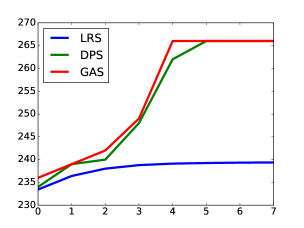
(a) $LRS,DPS$ and $GAS$ solutions.

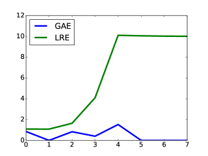
(b) $GAE$ and $LRE$ efficiencies.

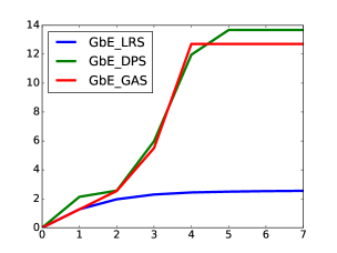
(c) $GbE_{LRS},GbE_{DPS}$ and $GbE_{GAS}$ efficiencies.

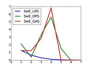
(d) $SwE_{LRS},SwE_{DPS}$ and $SwE_{GAS}$ efficiencies.

Figure 4: Example 1. Random realization of 128 eligible items, with uniformly distributed capacities and demand-capacity fraction of 0.9. The D&C tree has height 7, it is generated by the head-left algorithm 3, sorted by specific weight $\bm{\gamma}$, left subtree fraction $f=0.5$ and minimum size $m=1$. In Figure (a) the $y$-axis is expressed in absolute values while in figures (b), (c) and (d) the $y$-axis is a percentage.

Finally, in Figure 5 we present the efficiencies $GbE_{DPS},SwE_{DPS},GAE$ and $LRE$ for five random realizations. We choose depicting this efficiencies because the Exact Solution ($DPS$) is the most important parameter, as it measures the quality of the exact solution and the $GAE$, $LRE$ efficiencies store the quality of the usual bounds (Greedy Algorithm and Linear Relaxation). The realizations are generated with the same parameters of the previous one (therefore comparable to it) and follow similar behavior amongst them as expected. In particular, notice that for $h\geq 4$ (subproblems of size $8$ or smaller) the solutions stabilize.

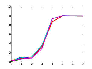
(a) $LRE$ efficiencies.

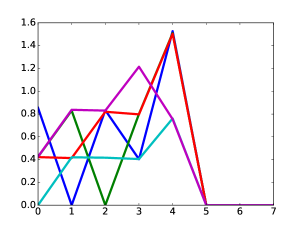
(b) $GAE$ efficiencies. (Different line styles are used to help the reader identify the path that each random realization follows.)

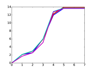
(c) $GbE_{DPS}$ efficiencies.

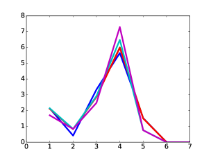
(d) $SwE_{DPS}$ efficiencies.

Figure 5: Example 1. Five random random realization of 128 eligible items, with uniformly distributed capacities and demand-capacity fraction of 0.9. The D&C tree has height 7, it is generated by the head-left algorithm 3, sorted by specific weight $\bm{\gamma}$, left subtree fraction $f=0.5$ and minimum size $m=1$.

Remark 10.

Examples of 128 eligible items, with a large number of realizations and different distributions (uniform, binomial, Poisson) present similar behavior to the one presented in Example 1. For the three distributions, most of the results stabilize for $h\geq 4$ (subproblems of $8$ items).

5 Numerical Experiments

In this section, we present the results from the numerical experiments. All the codes needed for the present work were implemented in Python 3.4 and the databases were handled with Pandas (Python Data Analysis Library). The full scale experiments were run in the server Gauss at Universidad Nacional de Colombia, Sede Medellín, Facultad de Ciencias. The Script can be downloaded from the address https://sites.google.com/a/unal.edu.co/fernando-a-morales-j/home/research/software

5.1 The Experiments Design

The numerical experiments are aimed to asses the effectiveness of the heuristic D&C method presented in Section 4. Its whole construction was done in a way such that its effectiveness could be analyzed under the probabilistic view of the Law of Large Numbers (which we write below for the sake of completeness, its proof and details can be found in [2]).

Theorem 7 (Law of Large Numbers).

Let $\big{(}\mathsf{Z}^{(n)}:n\in\bm{\mathbbm{N}}\big{)}$ be a sequence of independent, identically distributed random variables with expectation $\bm{\mathbb{E}}\big{(}\mathsf{Z}^{(1)}\big{)}$, then

$$\bm{\mathbbm{P}}\bigg{[}\Big{|}\frac{\mathsf{Z}^{(1)}+\mathsf{Z}^{(2)}+\ldots+\mathsf{Z}^{(n)}}{n}-\bm{\mathbb{E}}\big{(}\mathsf{Z}^{(1)}\big{)}\Big{|}>0\bigg{]}\xrightarrow[n\,\rightarrow\,\infty]{}0,$$ (29)

i.e. , the sequence $\big{(}Z^{(n)}:n\in\bm{\mathbbm{N}}\big{)}$ converges to $\mu$ in the Cesàro sense.

The D&C method introduces several free/decision parameters to analyze the behavior of Problem 1 under different scenarios. We have the following list of domains for each of these parameters

1. Number of items: $N\in\bm{\mathbbm{N}}$.

2. Distribution of items’ capacities: $\operatorname*{\textit{dist}}\in\{\text{Ud, Pd, Bd}\}$ (Ud: uniform, Pd: Poisson, Bd: Binomial).

3. Demand-Capacity fraction: $o\in\{0,50,0.55,\ldots,0,90\}$ (to satisfy hypotheses of (iv) Theorem 5).

4. Price-Capacity rate: $r\in\{34,44,54,64,74\}$ (to avoid hypotheses of Theorem 3 been satisfied).

5. D&C tree algorithm $\operatorname*{\textit{T-alg}}\in\{\text{hlT, blT}\}$ (hlT head-left Tree Algorithm 3, blT balanced-left Tree Algorithm 5).

6. Eligible Items list sorting method: $s\in\{\bm{p},\bm{c},\bm{\gamma},\text{random}\}$.

7. Fraction of the left list: $f\in\{0.35,0.40,\ldots,0.65\}$.

8. Minimum list size: $m\in\bm{\mathbbm{N}}$.

Remark 11 (Parameters Domains).

It is clear that $o$ and $f$ could very well adopt any value inside the interval $[0.1]$, while $r$ could be any arbitrary number in $\bm{\mathbbm{N}}$. However, adopting such ranges is impractical for two reasons. First, their infinite nature prevents an exhaustive exploration as we intend to do. Second, most of the values in such a large range are unrealistic. For instance: $o=0.1$ means that the capacity of available items is 10 times the demand (scenario that will hardly occur in real-world problems), $f=0$ means no D&C pair was introduced and $r\geq\max_{i\,\in\,[N]}c_{i}$ means that all the items have the same price regardless of their capacity.

In order to model, an integer problem of type 1 and its D&C solution as random variables, we need to introduce the following definition

Definition 9.

Consider the following probabilistic space and random variables.

1. Denote by $\Omega$ the set of all possible integer problems of the type 1.

2. Define the random problem generator variable as

   $$\begin{split}\mathsf{X}:\bm{\mathbbm{N}}\times\{\text{Ud, Pd, Bd}\}\times\{0,50,0.55,\ldots,0,90\}\rightarrow&\Omega\\ (N,\operatorname*{\textit{dist}},o)\mapsto&\mathsf{X}(N,\operatorname*{\textit{dist}},o).\end{split}$$ (30)

   Here, $\mathsf{X}(N,\operatorname*{\textit{dist}},o)$ is an integer problem of type 1.

3. Define the D&C solution variable by

   $$\begin{split}\mathsf{S}:\Omega\times\{34,44,\ldots,74\}\times\{\text{hlT, blT}\}\times\{0.35,0.40,\ldots,0.65\}\times\\ \{\bm{p},\bm{c},\bm{\gamma},\text{random}\}\times\bm{\mathbbm{N}}\rightarrow&\bigcup\limits_{h\,\in\,\bm{\mathbbm{N}}}\bm{\mathbbm{N}}^{h}\\ (\mathsf{X},r,\operatorname*{\textit{T-alg}},s,f,m)\mapsto&\mathsf{S}(\mathsf{X},r,\operatorname*{\textit{T-alg}},s,f,m).\end{split}$$ (31)

   In the expression above, it is understood that $\mathsf{X}=\mathsf{X}(N,dist,o)$ is the random problem generator variable and $\mathsf{S}(\mathsf{X},r,\operatorname*{\textit{T-alg}},s,f,m)$ indicates the solution for the chosen integer problem $\mathsf{X}\in\Omega$, under the D&C tree solution parameters $r,\operatorname*{\textit{T-alg}},s,f,m$. This is, a stack/vector of solutions in $\bm{\mathbbm{N}}^{\mathsf{H}}$ where $\mathsf{H}$ is the height of the constructed D&C tree. In particular, notice that $\mathsf{H}$ is also a random variable.

Notice that if the parameters $N,s,m$ are fixed, then, $\mathsf{H}$ is constant and the D&C solutions random variable $\mathsf{S}\big{(}\mathsf{X}(N,dist,o),r,\operatorname*{\textit{T-alg}},s,f,m\big{)}\in\bm{\mathbbm{N}}^{\mathsf{H}}$. However, a Monte Carlo simulation analysis can not be applied under these conditions, because the realizations of the random variable $\mathsf{S}$ would not meet the hypotheses of the Law of Large Numbers 7, more specifically, the identically distributed condition. On the other hand, the analysis is pertinent for several realizations of the random variables $\mathsf{X}$ and $\mathsf{S}$, with a fixed list of free/decision parameters, namely $P=(N,dist,o,r,\operatorname*{\textit{T-alg}},s,f,m)$. Under these conditions the Law of Large Numbers can be applied on $\mathsf{S}$ to estimate the expected effectiveness of the method, conditioned to the chosen set of parameters $P$.

In order to compare the different scenarios without introducing too many possibilities a standard setting has to be defined, which we introduce below, together with the justification behind its choice.

Definition 10.

In the following we refer to the standard setting of a numerical experiment

$$P=\begin{cases}(N,dist,o,r,\operatorname*{\textit{T-alg}},s,f,m),&\text{for }\operatorname*{\textit{T-alg}}=\text{hlT},\\ (N,dist,o,r,\operatorname*{\textit{T-alg}},s,m),&\text{for }\operatorname*{\textit{T-alg}}=\text{blT},\end{cases}$$

if its parameters satisfy the following values:

1. Head Fraction, $f=0.5$ (applies for the head-left method only). To make it comparable with the balanced method.

2. Demand-Capacity Fraction, $o=0.9$.

3. Price-Capacity rate, $r=54$. From experience, this is a reasonable value, as it permits explore problems of computable size without landing into trivial scenarios.

4. Eligible Items list sorting method, $s=\bm{\gamma}$ i.e., specific weight. Because this greedy function is closely related to the solutions furnished by the linear relaxation (LRS), presented in Theorem 2, as well as the Greedy Algorithm 1.

5. Minimum list size, $m=4$. From multiple random realizations, it has been observed that the D&C method does not yield significantly different results for list sizes smaller than $m=8$; see Remark 10. Consequently, we adopt the size $m=4$ in order to capture one step (and only one) of this “steady behavior”.

6. Number of eligible items, $N=512$. This size was chosen because for $m=4$ it will produce in most of the studied cases a D&C tree of height $7$. The only exceptions will occur for head-left generated trees with head fraction $f\neq 0.5$.

In addition the next conventions are adopted

1. An experiment is defined by a list of parameters, namely $P$; from now on we do not make a distinction between the experiment and its list of parameters. Moreover, $P$ has 8 parameters if $\operatorname*{\textit{T-alg}}=\text{hlT}$ and 7 if $\operatorname*{\textit{T-alg}}=\text{blT}$. To ease notation, from now on we denote $P=(512,\operatorname*{\textit{dist}},o,r,\operatorname*{\textit{T-alg}},s,f,4)$ for any experiment in general, in the understanding that if $\operatorname*{\textit{T-alg}}=\text{blT}$ the head fraction $f$ is not present in the list $P$.

2. Each case will be analyzed using $50$ randomly generated realizations of $512$ items with Uniform, Poisson and Binomial distributions respectively i.e., $P=(512,dist,o,r,\newline \operatorname*{\textit{T-alg}},s,f,4)$, see Figure 6.

3. Given a standard setting $P=(512,dist,o,r,\operatorname*{\textit{T-alg}},s,f,4)$ and a variable $v\in\{o,r,s,f\}$, we denote by $P(v)$ the list of experiments where the variable $v$ runs through its whole domain, see Table 11 and Figure 7 .

4. The analysis of the efficiencies $GAE,LRE,GbE_{LRS},GbE_{DPS},GbE_{GAS},SwE_{LRS}$, $SwE_{DPS}$ and $SwE_{GAS}$ will be done using their average values, corresponding to the 50 random realizations mentioned above. In the following, we denote by $\mathcal{E}$ the list ot these efficiencies; due to the Law of Large Numbers 7 we know this is an approximation of their expected values. An example is presented in Table 11 and Figure 7 below.

Figure 6: Schematics of the set of numerical experiments in search of optimal strategies. The first level, depicted in Figure (a), branches on the tree generation method: lhT and blT. The second level branches on the remaining strategies: $o$, $r$, $s$ for both $\{\text{lhT},\text{blT}\}$ and $f$ for the lhT method. Figure (b) displays the branching process for the blT method; a similar diagram corresponds for the lhT method.

5.2 Critical Height and hlT vs. blT strategies Comparison

As a first step we find a critical height. From the numerical experiments, it is observed that the method heavily deteriorates beyond certain height i.e., after certain number of D&C iterations, as it can be seen in the figures 4 and 5 from Example 1, where it can be observed that beyond $h>3$ the slope becomes very steep, therefore a critical height needs to be adopted.

Definition 11.

Given an experiment of 50 realizations with a fixed set of parameters $P=(512,dist,o,r,\operatorname*{\textit{T-alg}},s,f,4)$ and let $v\in\{o,r,s,f\}$ be a variable running through its full domain. Define

1. For a fixed efficiency $\operatorname*{\textit{eff}}\in\mathcal{E}$, denote respectively $\bar{\mathsf{S}}(\operatorname*{\textit{eff}},P)$, $\bar{\mathsf{S}}(\operatorname*{\textit{eff}},P,v)$, the average value of 50 random realizations executed with parameters $P$ and the list of such values when the variable $v$ runs through its whole domain, see Table 11 and Figure 7 below.

2. For a fixed efficiency $\operatorname*{\textit{eff}}\in\mathcal{E}$, denote by

   $$\bar{\mathsf{S}}^{\prime}(\operatorname*{\textit{eff}},P,v)(h)\overset{\mathbf{def}}{=}\bar{\mathsf{S}}(\operatorname*{\textit{eff}},P,v)(h)-\bar{\mathsf{S}}(\operatorname*{\textit{eff}},P,v)(h-1), \text{for }h=1,2,\ldots,H,$$

   with $H$ the height of the D&C tree. Denote by $\bar{\mathsf{S}}^{\prime}_{v}(\operatorname*{\textit{eff}},P)(h)=\max\{\bar{\mathsf{S}}^{\prime}(\operatorname*{\textit{eff}},P,v)(h):v\,\in\,\text{full domain}\}$.

3. For each of the efficiencies $\operatorname*{\textit{eff}}\in\mathcal{E}$, its critical height relative to the variable $v$, denote by $h_{v}(\operatorname*{\textit{eff}},P)$ the last height $h$ satisfying $\bar{\mathsf{S}}^{\prime}_{v}(\operatorname*{\textit{eff}},P)(h)\leq 2\bar{\mathsf{S}}^{\prime}_{v}(\operatorname*{\textit{eff}},P)(h-1)$, see Table 11 and Figure 7.

4. The critical height of the experiment relative to the variable $v$, denoted by $h_{v}(P)$ is given by the mode of the list $\{h_{v}(\operatorname*{\textit{eff}},P):\operatorname*{\textit{eff}}\in\mathcal{E}\}$.

5. In order to compare the experiments $P_{\text{hlT}}=(512,dist,o,r,\text{hlT},s,0.5,4)$ and $P_{\text{blT}}=(512,dist,o,r,\text{lbT},s,4)$ (head-left vs balanced), relative to the variable $v$, we proceed as follows: set the height $\tilde{h}\overset{\mathbf{def}}{=}\min\{h_{v}(P_{\text{{hlT}}}),h_{v}(P_{\text{{blT}}})\}$ (see Table 13) and compute the $\ell^{1}$-norm for the arrays $\{\bar{\mathsf{S}}(\operatorname*{\textit{eff}},P_{\text{hlT}},v)(h):\operatorname*{\textit{eff}}\in\mathcal{E},\,h=1,2,\ldots,\tilde{h}\}$, $\{\bar{\mathsf{S}}(\operatorname*{\textit{eff}},P_{\text{blT}},v)(h):\operatorname*{\textit{eff}}\in\mathcal{E},\,h=1,2,\ldots,\tilde{h}\}$, when regarded as lists (not as matrices, as Table 11 would suggest). The lowest of these norms yields the best strategy among hlT and blT.

Example 2.

In the table 11 below we display $\{\bar{\mathsf{S}}(GbE_{DPS},P,r)(h):h=0,1,\ldots,7\}$ i.e., the averaged values corresponding to 50 realizations for the efficiency $\operatorname*{\textit{eff}}=GbE_{DPS}$ running through the full domain of the price-capacity rate i.e., $v=r$. The list of parameters is given by $P=(512,\text{Ud},0.9,r,\text{hlT},\bm{\gamma},0.5,4)$ with $r\in\{34,44,54,64,74\}$. The tables corresponding to the intermediate slope variables $\{\bar{\mathsf{S}}^{\prime}(P,v)(h):h=0,1,\ldots 7\}$, $\{\bar{\mathsf{S}}^{\prime}_{v}(P)(h):h=0,1,\ldots 7\}$ are omitted since they can be completely deduced from Table 11. In this particular example $h_{v}(\operatorname*{\textit{eff}})=h_{r}(GbE_{DPS})=5$.

Height	$r=34$	$r=44$	$r=54$	$r=64$	$r=74$
0	0.00	0.00	0.00	0.00	0.00
1	1.26	1.93	1.95	2.29	1.82
2	2.11	3.19	3.40	3.45	2.74
3	2.66	3.91	4.27	4.34	3.53
4	3.15	4.52	4.85	4.92	4.17
➙ $h_{r}(P)=5$	3.93	5.68	6.63	7.08	6.24
6	7.72	9.56	10.11	9.99	8.74
7	14.11	15.50	15.70	15.66	14.83

Table 11: Average values of 50 random realizations for the efficiency variable $\operatorname*{\textit{eff}}=GbE_{DPS}$ relative to the variable $v=r$. The experiments parameters $P=(N,dist,o,r,\operatorname*{\textit{T-alg}},s,f,m)$ have the following values: $N=512$, $\operatorname*{\textit{dist}}=\text{Ud}$, $o=0.9$, $r\in\{34,44,54,64,74\}$, $\operatorname*{\textit{T-alg}}=\text{hlT}$, $s=\bm{\gamma}$, $f=0.5$, $m=4$.

Finally, the corresponding solution is presented in Figure 7 (a), together with its analogous for the efficiencies $SwE_{DPS},GAE,LRE$ ((b), (c) and (d) respectively). We chose to present these efficiencies because the Exact Solution behavior $DPS$, is the central parameter to asses the quality of the method for measuring the quality of the solution, while the efficiencies $GAE,LRE$ measure the expected quality of the usual bounds (Greedy Algorithm and Linear Relaxation) through the D&C tree.

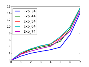
(a) $\bar{\mathsf{S}}(GbE_{DPS},P,r)$, $r\in\{34,44,54,64,74\}$.

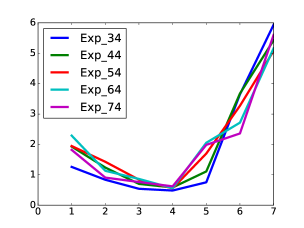
(b) $\bar{\mathsf{S}}(SwE_{DPS},P,r)$, $r\in\{34,44,54,64,74\}$.

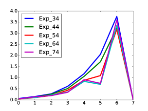
(c) $\bar{\mathsf{S}}(GAE,P,r)$, $r\in\{34,44,54,64,74\}$.

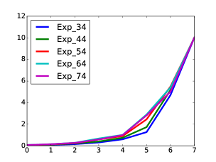
(d) $\bar{\mathsf{S}}(LRE,P,r)$, $r\in\{34,44,54,64,74\}$.

Figure 7: Example 2. Averaged values for 50 random realizations. Four particular efficiencies are depicted $GbE_{DPS},SwE_{DPS},GAE,LRE$. The notation $\text{Exp}\_{r}$ with $r\in\{34,,44,54,64,74\}$ in the graphics’ legends, stands for the expected value for the corresponding $\bar{\mathsf{S}}(\operatorname*{\textit{eff}},P,r)$, $\operatorname*{\textit{eff}}\in\{GbE_{DPS},SwE_{DPS},GAE,LRE\}$.

Given that the aim of this section is to compare the generation methods hlT vs. blT, we first find the optimal head fraction value $f$ for hlT, in order to attain the best possible efficiencies for the hlT method. The results are summarized in Table 12 below; the pointing arrows indicate the optimal head fraction values

Head Fraction	Uniform		Poisson		Binomial
$f$	Height $h_{o}(P_{\text{blT}})=4$		Height $h_{o}(P_{\text{blT}})=3$		Height $h_{o}(P_{\text{blT}})=3$
	$GbE_{DPS}$	$\operatorname*{\textit{eff}}\in\mathcal{E}$	$GbE_{DPS}$	$\operatorname*{\textit{eff}}\in\mathcal{E}$	$GbE_{DPS}$	$\operatorname*{\textit{eff}}\in\mathcal{E}$
0.35	➙ 8.27	➙ 26.45	2.83	8.87	➙ 3.36	➙ 10.54
0.40	8.88	28.20	3.06	9.60	3.54	11.04
0.45	9.30	29.43	2.87	8.97	3.69	11.56
0.50	9.62	30.51	2.94	9.27	3.67	11.49
0.55	9.72	30.57	2.95	9.30	4.02	12.51
0.60	9.64	30.48	3.12	9.78	4.23	13.12
0.65	9.73	30.63	➙ 2.82	➙ 8.81	4.16	13.06

Table 12: Head Fraction Comparison. Table registering values of $\ell^{1}$-norms of arrays $\{\bar{\mathsf{S}}(\operatorname*{\textit{eff}},P_{\text{blT}},f)(h):\operatorname*{\textit{eff}}\in\mathcal{E},\,h=1,2,\ldots,h_{f}(P_{\text{blT})}\}$ and $\{\bar{\mathsf{S}}(GbE_{DPS},P_{\text{blT}},f)(h):h=1,2,\ldots,h_{f}(P_{\text{blT}})\}$. The values are displayed for $f\in\text{full domain}$ and $\operatorname*{\textit{dist}}\in\{\text{Ub, Pd, Bd}\}$. The remaining parameters are $o=0.9$, $r=54$, $s=\bm{\gamma}$ and Minimum List Size $m=4$ i.e., $P_{\text{hlT}}=(512,dist,o,54,\text{hlT},\bm{\gamma},0.5,4)$. The pointing arrows indicate the optimal strategy within its column or family of comparable experiments.

Remark 12.

As it can be observed in Table 12, the optimal values are attained at the extremes of the head fraction experimental range and this happens in the three distributions in analysis. This is hardly surprising, as a bigger head (for the Poisson distribution) or a bigger tail (for the Uniform and Binomial distributions) have a better chance to capture a big chunk of a real optimal solution. Furthermore, when the range of head fraction is extended, namely if we take $[a,b]\subseteq[0,1]$ such that $[0.35,0.65]\subsetneq[a,b]$, the optima occur at the extremes $a$ and $b$. In particular for $f\in\{0,1\}$ we are back in the original problem and attaining the original optima with the original computational complexity, which defeats the purpose of the D&C method itself.

Adopting the optimal heights for the lhT method and recalling the definitions above, the list of critical heights is summarized in the table 13 below. The pointing arrows indicate the comparison height between hlT and blT tree generation methods.

Var	Uniform, $f=0.35$		Poisson, $f=0.65$		Binomial, $f=0.35$
$v$	Head-Left	Balanced	Head-Left	Balanced	Head-Left	Balanced
$o$	5	➙ 4	4	➙ 3	➙ 4	➙ 4
$r$	➙ 5	➙ 5	➙ 2	3	➙ 2	3
$s$	➙ 4	6	➙ 3	4	➙ 3	5

Table 13: Critical Heights table. Each corresponds to the expected values of efficiencies $\mathcal{E}$ coming from the experiments with parameters $P=(512,dist,o,r,\text{lfT},s,f,4)$ ($f=0.35$ for $\operatorname*{\textit{dist}}\in\{\text{Ud, Bd}\}$, $f=0.65$ for $\operatorname*{\textit{dist}}=Pd$) or $P=(512,dist,o,r,\text{blT},s,4)$. The heights pointed with arrows are the values valid for comparison between the lfT and blT tree generation methods.

Once the heights’ comparison values are found, we proceed to compare both methods in analogous conditions i.e., when the remaining variables are equal. The results for the demand-capacity fraction variable $o$, running through its full domain, are summarized in Table 14. Similar tables were constructed for the price-capacity rate $r\in\{34,44,54,64,74\}$ and the sorting $s\in\{\bm{p},\c{,}\bm{\gamma},\text{random}\}$ variables running through their respective full domains which we omit here for the sake of brevity.

It is important to notice that in Table 14 all the values corresponding to the blT method are lower than its corresponding analogous for the hlT algorithm. The same phenomenon can be observed for the table running through the price-capacity rate $r$. The table running through the sorting variable also shows clear predominance of the blT over the hlT method, though it is not absolute (10 out of 12 cases) as in the previous cases. Furthermore, noticing the differences of values, it follows that blT produces significant better results than hlT. Therefore, this choice of strategy when using the D&C approach is clear and the remaining strategies need to be decided based on blT tree generation algorithm results.

Remark 13 (Head Fraction $f$ values).

With regard to the optimal head fraction values it is important to notice the following

1. As expected, the optimal values tend to be on the extremes $f=0.35$ or $f=0.65$, since $f=0$ or $f=1$ would imply that no D&C pair has been introduced and therefore the efficiency should be 100%.

2. Notice that hlT generated D&C tree for $f\neq 0.5$ will be deeper than its analogous for blT, see Figures 1, 2 and 3. In particular, the hlT method with optimal head fraction values ($f=0.35$, $f=0.65$) has higher complexity than its blT analogous.

3. A similar comparison procedure was done between hlT and blT, when $f=0.5$ i.e., the standard. As expected, the hlT yields poorer results than using the optimal head fraction values and blT is remarkably superior.

Occupancy	Uniform		Poisson		Binomial
$o$	Comparison Height $\tilde{h}=4$		Comparison Height $\tilde{h}=3$		Comparison Height $\tilde{h}=4$
	Head-Left	Balanced	Head-Left	Balanced	Head-Left	Balanced
	$f=0.35$		$f=0.65$		$f=0.35$
0.50	98.66	7.19	35.51	3.12	49.59	7.00
0.55	86.04	7.69	32.95	2.65	44.37	5.64
0.60	74.47	7.57	29.20	2.58	40.19	5.86
0.65	64.25	6.73	25.35	2.42	37.71	5.33
0.70	55.42	6.16	21.83	2.01	34.41	4.46
0.75	47.39	5.56	18.61	1.77	30.73	4.56
0.80	40.53	5.13	15.58	2.09	27.25	3.81
0.85	34.35	3.74	12.57	2.30	23.93	4.00
0.90	26.45	3.81	8.81	2.08	18.83	4.11

Table 14: Occupancy Fraction Comparison. Table registering values of $\ell^{1}$-norms of arrays $\{\bar{\mathsf{S}}(\operatorname*{\textit{eff}},P_{\operatorname*{\textit{T-alg}}},o)(h):\operatorname*{\textit{eff}}\in\mathcal{E},\,h=1,2,\ldots,\tilde{h}\}$ for $o\in\text{full domain}$, $\operatorname*{\textit{T-alg}}\in\{\text{hlT},\text{blT}\}$ and $\operatorname*{\textit{dist}}\in\{\text{Ub, Pd, Bd}\}$. The remaining parameters are $r=54$, $s=\bm{\gamma}$, Left Head Fraction $f=0.35$ for $\operatorname*{\textit{dist}}\in\{\text{Ud, Bd}\}$, $f=0.65$ for $\operatorname*{\textit{dist}}=Pd$ (if $\operatorname*{\textit{T-alg}}=\text{hlT}$) and Minimum List Size $m=4$ i.e., $P=(512,dist,o,54,\operatorname*{\textit{T-alg}},\bm{\gamma},f\in\{0.35,0.65\},4)$. Observe that in all the instances of the problems, the blT method gives better results than the hlT.

5.3 Optimal Strategies

In the previous section, it was determined that blT produces better results than hlT. Consequently, from now on, we focus on finding the best values for the remaining parameters: $o$, $r$ and $s$ conditioned to the blT tree generation method.

First we revisit the pruning height of the tree: given that $\tilde{h}\leq h_{v}(P_{\text{blT}})$ (as introduced in Definition 11 (v)) and the analysis is now narrowed down to the blT method, the computations will be done for these heights because is desirable to stretch the D&C method as far as possible but within the quality deterioration control established by $h_{v}(P_{\text{blT}})$ (see Definition 11 (iv)).

Second, now we analyze the method from two points of view. A global one, as it has been done so far accounting for the overall efficiency of the variables in $\mathcal{E}$ by computing the $\ell^{1}$-norm of the array $\{\bar{\mathsf{S}}(\operatorname*{\textit{eff}},P_{\text{blT}},v)(h):\operatorname*{\textit{eff}}\in\mathcal{E},\,h=1,2,\ldots,\tilde{h}\}$ as introduced in Definition 11 (v). A specialized and second point of view, uses only the $\ell^{1}$-norm of the array $\{\bar{\mathsf{S}}(GbE_{DPS},P_{\text{blT}},v)(h):h=1,2,\ldots,\tilde{h}\}$ i.e., regarding only the behavior of the efficiency $GbE_{DPS}$, through the variables $o$, $r$ and $s$. This specialized measurement is presented because the efficiency of the Exact Solution ($DPS$) is the most important parameter, given that it contains the behavior of the exact solution.

In Table 15 below the $GbE_{DPS}$ and the global efficiency $\operatorname*{\textit{eff}}\in\mathcal{E}$ are presented for the demand-capacity fraction variable $o$, running through its full domain. The pointing arrows indicate the optimal strategy within its column or family of comparable experiments. As in the previous stage, similar tables were built for the price-capacity rate $r\in\{34,44,54,64,74\}$ and the sorting $s\in\{\bm{p},\bm{c},\bm{\gamma},\,\text{random}\}$ variables, running through their respective full domains, which we omit here for the sake of brevity. Finally, in the tables 16 and 17 below we summarize the optimal strategies from both points of view, the specialized $GbE_{DPS}$ and the global one $\operatorname*{\textit{eff}}\in\mathcal{E}$.

Occupancy	Uniform		Poisson		Binomial
$o$	Height $h_{o}(P_{\text{blT}})=4$		Height $h_{o}(P_{\text{blT}})=3$		Height $h_{o}(P_{\text{blT}})=4$
	$GbE_{DPS}$	$\operatorname*{\textit{eff}}\in\mathcal{E}$	$GbE_{DPS}$	$\operatorname*{\textit{eff}}\in\mathcal{E}$	$GbE_{DPS}$	$\operatorname*{\textit{eff}}\in\mathcal{E}$
0.50	1.28	7.19	0.67	3.12	1.83	7.00
0.55	1.14	7.69	0.58	2.65	1.35	5.64
0.60	1.08	7.57	0.50	2.58	1.30	5.86
0.65	0.95	6.73	0.54	2.42	1.29	5.33
0.70	0.87	6.16	➙ 0.33	2.01	1.00	4.46
0.75	0.79	5.56	0.42	➙ 1.77	0.98	4.56
0.80	➙ 0.75	5.13	0.50	2.09	0.82	➙ 3.81
0.85	➙ 0.75	➙ 3.74	0.52	2.30	0.78	4.00
0.90	0.84	3.81	0.56	2.08	➙ 0.62	4.11

Table 15: Occupancy Fraction Comparison. Table registering values of $\ell^{1}$-norms of arrays $\{\bar{\mathsf{S}}(\operatorname*{\textit{eff}},P_{\text{blT}},o)(h):\operatorname*{\textit{eff}}\in\mathcal{E},\,h=1,2,\ldots,h_{o}(P_{\text{blT}}\}$ and $\{\bar{\mathsf{S}}(GbE_{DPS},P_{\text{blT}},o)(h):h=1,2,\ldots,h_{o}(P_{\text{blT}})\}$. The values are displayed for $o\in\text{full domain}$ and $\operatorname*{\textit{dist}}\in\{\text{Ub, Pd, Bd}\}$. The remaining parameters are $r=54$, $s=\bm{\gamma}$ and Minimum List Size $m=4$ i.e., $P=(512,dist,o,54,\text{blT},\bm{\gamma},4)$. The pointing arrows indicate the optimal strategy within its column or family of comparable experiments.

Var	Uniform			Poisson			Binomial
$v$	Strategy	Height	Error	Strategy	Height	Error	Strategy	Height	Error
		$h_{v}(P_{\text{blT}})$	$\ell^{1}$		$h_{v}(P_{\text{blT}})$	$\ell^{1}$		$h_{v}(P_{\text{blT}})$	$\ell^{1}$
$o$	0.80/0.85	4	0.75	0.70	3	0.33	0.90	4	0.62
$r$	34	5	1.08	34	3	0.22	34	3	0.15
$s$	$\bm{c}$	6	2.85	random	4	1.07	$\bm{c}$	5	1.01

Table 16: Chosen Strategies Table. Summary of best strategies. The expected errors are measured with the $\ell^{1}$-norms of arrays $\{\bar{\mathsf{S}}(GbE_{DPS},P_{\operatorname*{\textit{T-alg}}},v)(h):h=1,2,\ldots,h_{v}(P_{\text{blT}})\}$, for each of the variables $v\in\{o,r,s\}$. These were used as decision parameters; given that the norms are computed only for the $BgE_{DPS}$ efficiency, this point of view only considers the exact solution. The tree generation method is the blT since it was determined as the best tree generation strategy.

Var	Uniform			Poisson			Binomial
$v$	Strategy	Height	Error	Strategy	Height	Error	Strategy	Height	Error
		$h_{v}(P_{\text{blT}})$	$\ell^{1}$		$h_{v}(P_{\text{blT}})$	$\ell^{1}$		$h_{v}(P_{\text{blT}})$	$\ell^{1}$
$o$	0.85	4	3.74	0.75	3	1.77	0.80	4	3.81
$r$	44	5	6.77	34	3	1.69	64	3	1.06
$s$	$\bm{\gamma}$	6	12.29	$\bm{\gamma}$	4	3.79	$\bm{\gamma}$	5	8.52

Table 17: Summary of Chosen Strategies. In this case the expected errors are measured with the $\ell^{1}$-norms of arrays $\{\bar{\mathsf{S}}(\operatorname*{\textit{eff}},P_{\operatorname*{\textit{T-alg}}},v)(h):\operatorname*{\textit{eff}}\in\mathcal{E},\,h=1,2,\ldots,h_{v}(P_{\text{blT}})\}$, for each of the variables $v\in\{o,r,s\}$. These were used as decision parameters; given that the norms are computed through all the efficiencies in $\mathcal{E}$, this a global point of view. The tree generation method is the blT since it was determined as the best tree generation strategy.

5.4 Computational Time

In this section, we discuss the computational time needed for the Divide & Conquer method. To that end, we present the relative times rather than the absolute computational times, as the latter values can greatly vary from one computer to another. More specifically we focus on the relative computational global time (GbT) and stepwise time (SwT), introduced in Definition 8, equations (25a), (25b).

In the tables 18 we display the expected values of $GbT$ and $SwT$ (after 50 realizations) of the Exact Solution ($DPS$), for the datasets generated by the three random distributions and taking the problems in standard setting (see Definition 10), the corresponding graphs are depicted in Figures 8 (a), (b). In the same fashion, Table 19 and Figures 8 (c), (d), summarize the expected values for $GbT$ and $SwT$ when measuring the computational time of the Linear Relaxation Solution ($LRS$). The Greedy Approximation Solution ($GAS$) presents an analogous behavior to the $LRS$, which we omit here for brevity. As it can be observed in both, the table and figures, the difference in computational time is marginal, but is strongly tied to the algorithm that must be solved along the D&C tree. Moreover, a similar phenomenon will be observed when moving away from the standard setting to the other problem instances explored before (see Figure 6 ), i.e., the computational time is essentially indifferent with respect to the D&C strategies and the data distribution.

Height	Uniform		Poisson		Binomial
	$GbT$	$SwT$	$GbT$	$SwT$	$GbT$	$SwT$
0	100		100		100
1	46.93	46.93	47.42	47.42	45.69	45.69
2	25.47	54.29	26.26	55.37	24.61	53.86
3	15.97	62.70	16.74	63.76	15.05	61.15
4	11.51	72.05	12.35	73.82	10.65	70.80
5	8.94	77.68	9.66	78.23	8.09	76.00
6	7.88	88.21	8.66	89.59	7.10	87.79
7	8.39	106.39	9.23	106.64	7.53	106.03

Table 18: Summary of Computational Times Exact Solution ($DPS$). See equations (25a), (25b) for the definitions of $GbT$ and $SwT$ respectively. See Figures 8 (a), (b) for their corresponding depiction.

Height	Uniform		Poisson		Binomial
	$GbT$	$SwT$	$GbT$	$SwT$	$GbT$	$SwT$
0	100		100		100
1	42.60	42.60	46.76	46.76	46.23	46.23
2	24.95	58.59	25.81	55.20	25.41	54.97
3	17.66	70.80	17.75	68.77	17.74	69.85
4	13.66	77.37	13.96	78.65	13.97	78.76
5	12.72	93.16	13.20	94.58	13.28	95.09
6	12.83	100.90	14.13	107.04	14.20	106.92
7	14.79	115.20	15.60	110.44	15.78	111.16

Table 19: Summary of Computational Times Linear Relaxation Solution. See equations (25a), (25b) for the definitions of $GbT$ and $SwT$ respectively. See Figures 8 (c), (d) for their corresponding depiction.

In the numerical results, we observe that the $DPS$ shows an exponential decay for the $BgT$, which is consistent with the almost linear behavior of the $SwT$. The critical $GbT$ point is $h=6$ because taking $h\geq 7$ would produce bigger computational time and a lower quality solution, i.e., deterioration in both features with respect to $h=6$. On the other hand, while the $LRS$ shows also an exponential decay, it has wilder behavior in the $SwT$ which scales up to a shift in the critical point $h=5$ in its $GbT$, i.e., for $h\geq 6$ there is no longer a trade-off between solution quality and computational time.

The existence of critical points in the $GbT$ mentioned above, occurs because some sizes of the problem are small enough for the algorithm ($DPS,LRS$ or $GAS$) to become quite efficient, therefore, the decomposition of a given problem in multiple parts such as the D&C tree generation, together with the reassembling of the problems’ results (computation of pruned trees, leaves and sums, see Definition 8), add up to higher computational times. Further experiments with different size for the original 0-1 Minimization KP are summarized in the table 20. From there, it follows that the D&C will continue to trade-off computational time vs. solution’s quality, until the size of the subproblems is 16 for the Exact Solution $DPS$ and 32 for the for the bounds $LRS,GAS$.

Problem	$LRS$		$DPS$		$GAS$
Size	Height	Size	Height	Size	Height	Size
128	3	32	4	16	3	32
256	4	32	5	16	4	32
512	5	32	6	16	5	32
1024	6	32	7	16	6	32

Table 20: Critical D&C tree Heights and associated subproblem sizes, for several sizes of the original 0-1 Minimization KP.

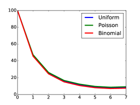
(a) Global Computational Time $GbT$, $DPS$. See Table 18.

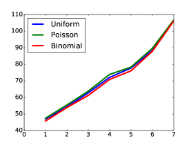
(b) Stepwise Computational Time $SwT$, $DPS$. See Table 18.

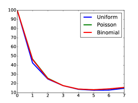
(c) Global Computational Time $GbT$, $LRS$. See Table 19.

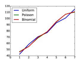
(d) Stepwise Computational Time $SwT$, $LRS$. See Table 19.

Figure 8: The figures display the average computational time values for 50 random realizations: global $GbT$ (see Equation (25a)) and Stepwise $SwT$ (see Equation (25b)). The Exact Solution $DPS$ (see Table 18) is depicted in figures (a), (b), while the Linear Relaxation Solution $LRS$ (see Table 19) is displayed in figures (c), (d). The experiments were done in the standard setting (see Definition 10). Other instances of the problem show similar behavior to its analogous in standard setting. The Greedy Approximation Solution (GAS) shows similar behavior to $LRS$.

6 Conclusions and Final Discussion

The present work yields the following conclusions. The heuristics of the method can be summarized as

1. We have proposed A Divide and Conquer method to solve the Knapsack Problem at large scale. The method reduces the computational time at the expense of loosing quality in the solution. Consequently, the central goal of the paper is to minimize the quality loss by finding the optimal strategies to use the method.

2. The deterioration of the solution’s accuracy and/or other parameters of control (such as upper and lower bounds) is defined as the efficiency of the method, and it is the main quantity to asses the quality of the method.

3. The method is heuristic therefore, several scenarios need to be explored in order to asses its efficiency. The scenarios are modeled using intermediate variables, some deterministic and some probabilistic, e.g. lhT, blT tree generation methods, distribution of capacities $\operatorname*{\textit{dist}}\in\{\text{Ud, Pd, Ud}\}$ respectively, see Figure 6.

4. The assessment of strategies is done statistically, using random realizations, computing the respective averages and appealing to the Law of Large Numbers 7 to approximate the expected behavior.

5. It is important to stress that the D&C method is not directly comparable with previous algorithms, because it does not compete with them, it complements them. In particular, approximation algorithms (such as those presented here or others included in [11] and [14]), essentially exact algorithms (such as COMBO from [13]) or exact algorithms (such as a naive Dynamic Programming implementation, or MT1 from [14]) can be combined with it. Matter of fact, it must be combined with a solution algorithm at certain level of branching if it is to produce an approximate solution at all.

From the results point of view

1. The D&C method can be applied several times to the original KP and generate a tree of subproblems, as those depicted in Figures 1, 2, 3. However, it is not reasonable to branch the problem producing subproblems smaller than $n=32$ (see Section 5.4) due to the trade-off between computational time and quality deterioration. Such limit is denoted by $h_{v}(P_{\text{blT}})$ and it constitutes the first strategy in applying the D&C method within a reasonable range of efficiency.

2. Two methods have been introduced to iterate the D&C heuristics, namely lhT, blT. They are compared after a common limit for the branching has been established: $\tilde{h}\overset{\mathbf{def}}{=}\min\{h_{v}(P_{\text{blT}}),h_{v}(P_{\text{hlT}})\}$. Next, the efficiencies of both methods are compared from three points of view: demand-capacity fraction (e.g. Table 14), price-capacity rate and sorting method. It follows that the blT furnishes significantly better results than the hlT in most of the possible scenarios.

3. Once the blT algorithm has been determined as the best tree/branching generation method, the remaining optimal strategies are searched from two points of view: a specialized one, focused on the exact solution only $GbE_{DPS}$, and a global one analyzing also the decay of the bounds of control $GAE,LRE$. The results are summarized in the tables 16 and 17 above.

4. As it can be seen, the optimal strategies disagree from one point of view to the other for most of the cases. It is useful to have these information for both cases because in practice, depending on the method to be used in solving the family of subproblems derived from successive applications of the D&C branching, it may be more convenient to prioritize one point of view over the other. For instance, if the family of subproblems will be solved using Exact, then $GbE_{DPS}$ is more important. On the other hand, if the method includes bounds control (quantified in $GAE$ and $LRE$) the global point of view may be preferable.

5. It is also important to stress that in most of the cases $GbE_{DPS}$ represents, in average, a fraction of 33% of the global efficiency. This shows that when applying the D&C method, the deterioration of the exact solution’s quality is important with respect to the deterioration of the bounds’ quality.

6. A paramount feature is that the D&C method deteriorates within reasonable values. In the case of $GbE_{DPS}$, a maximum expected error of $2.85\%$ is observed. However, such an error occurs after the 6th D&C iteration, which drastically reduces the computational time. On the other hand, the global quantification $\operatorname*{\textit{eff}}\in\mathcal{E}$, presents a quality decay of 12.29% in the worst case scenario but again, 6 D&C iterations were used and this value encompasses all the efficiencies. It follows that the proposed method is efficient.

7. The computational time is indifferent with respect to the strategies for the D&C tree design as well as the data probabilistic distribution.

The present paper opens up new research lines to be explored in future work

1. The reduction of computational time and critical problem sizes, discussed in Section 5.4, were quantified considering a serial algorithm implementation. A parallel implementation, on the other hand may furnish better results, because a D&C iteration produces two fully decoupled optimization problems. The assessment of computational time for a parallel scheme will be pursued in future work.

2. As mentioned above, currently a D&C iteration produces two fully decoupled subproblems. However, another scheme with partial coupling can be proposed namely introducing a pair of problems like that presented in Definition 5 (ii), Problem 4, but such that $A_{0}\cup A_{1}=[N]$ and $A_{0}\cap A_{1}\neq\emptyset$; with assigned demands $D_{0}$, $D_{1}$, computed by rules analogous to Equation (15) i.e., construct artificially an integer problem with the structure

   Problem 5 ($\Pi^{b},\,b=0,1$).

   $$\min\Bigg{[}\sum\limits_{b\,\in\,\{0,1\}}\sum\limits_{i\,\in\,A^{b}}p_{i}x_{i}-\sum\limits_{j\,\in\,A^{0}\cap A^{1}}p_{j}x_{j}\Bigg{]},$$ (32a)

   subject to

   $$\sum\limits_{i\,\in\,A^{0}}c_{i}x_{i}\geq D^{0}, \sum\limits_{i\,\in\,A^{1}}c_{i}x_{i}\geq D^{1}, x_{i}\in\{0,1\},\;\forall\,i\in[N].$$ (32b)

   A future line of research is the optimal choice of coupling/overlapping sets $A_{0}\cap A_{1}\neq\emptyset$ and exploit the structure of the integer programming problem 5 (analogously to the Dantzig-Wolfe decomposition for linear problems with the same structure). Furthermore, the optimality has to be analyzed from the perspective quality vs. computing time.

3. In this work, the method used a static choice of strategies, e.g. if the sorting method was $s=\bm{\gamma}$, it remained constant through all the nodes of the D&C tree (as Table 6, Figure 3 illustrate). A future line of research is to investigate the effect of mixing the strategies, e.g. the sorting parameter $s$ taking different values from $\{\bm{p},\bm{c},\bm{\gamma},\text{random}\}$ from one node to its children, or from one height (tree level) to the next.

4. The blT algorithm is significantly superior to the hlT method; the numerical evidence suggests that an analytic proof of this conjecture is plausible. A future line of research is to look for a rigorous mathematical proof, which of course, would use probability theory and furnish its results in terms of expected efficiencies.

5. Finally, a future line of research is the implementation and assessment of the D&C method for the optimization of general linear integer programs. However, such a step should be done only once the aforementioned aspects have been deeply studied.

References

• [1] Raul Baños, Consolación Gil, Julio Ortega, and Francisco G Montoya. Multilevel heuristic algorithm for graph partitioning. In Workshops on Applications of Evolutionary Computation, pages 143–153. Springer, 2003.
• [2] Patrick Billinsgley. Probability and Measure. Wiley Series in Probability and Mathematical Statistics. John Wiley $\&$ Sons, Inc., New York, NY, 1995.
• [3] Christian Blum, Jakob Puchinger, Günther R Raidl, and Andrea Roli. Hybrid metaheuristics in combinatorial optimization: A survey. Applied Soft Computing, 11(6):4135–4151, 2011.
• [4] Christian Blum and Andrea Roli. Metaheuristics in combinatorial optimization: Overview and conceptual comparison. ACM computing surveys (CSUR), 35(3):268–308, 2003.
• [5] Fred Glover and Saíd Hanafi. Tabu search and finite convergence. Discrete Applied Mathematics, 119(1):3 – 36, 2002. Special Issue devoted to Foundation of Heuristics in Combinatorial Optimization.
• [6] Jonathan L. Gross and Jay Yellen. Graph Theory and its Applications. Discrete Mathematics and its Applications. Chapman $\&$ Hall/CRC. Taylor $\&$ Francis Group, Boca Raton, FL, 2006.
• [7] Walter J. Gutjahr. A converging ACO algorithm for stochastic combinatorial optimization. In Andreas Albrecht and Kathleen Steinhöfel, editors, Stochastic Algorithms: Foundations and Applications, pages 10–25, Berlin, Heidelberg, 2003. Springer Berlin Heidelberg.
• [8] Walter J. Gutjahr. Convergence Analysis of Metaheuristics, pages 159–187. Springer US, Boston, MA, 2010.
• [9] Saíd Hanafi. On the convergence of tabu search. Journal of Heuristics, 7(1):47–58, Jan 2001.
• [10] Angel A Juan, Javier Faulin, Scott E Grasman, Markus Rabe, and Gonçalo Figueira. A review of simheuristics: Extending metaheuristics to deal with stochastic combinatorial optimization problems. Operations Research Perspectives, 2:62–72, 2015.
• [11] Hans Kellerer, Ulrich Pferschy, and David Pisinger. Knapsack Problems. Discrete Mathematics and its Applications. Springer, Berlin, Heidelberg, Ney York, 2004.
• [12] Edward Yu-Hsien Lin. A bibliographical survey on some well-known non-standard knapsack problems. INFOR: Information Systems and Operational Research, 36(4):274–317, 1998.
• [13] Silvano Martello, David Pisinger, and Paolo Toth. Dynamic programming and strong bounds for the 0-1 knapsack problem. Manage. Sci., 45(3):414–424, March 1999.
• [14] Silvano Martello and Paolo Toth. Knapsack Problems: Algorithms and Computer Implementations. Wiley-Interscience series in discrete mathematics and optimization. John Wiley & Sons Ltd., West Sussex, England, 1990.
• [15] David Pisinger. Where are the hard knapsack problems? Computers & Operations Research, 32(9):2271–2284, 2005.
• [16] S Voss, V Maniezzo, and T Stützle. Matheuristics: Hybridizing metaheuristics and mathematical programming (annals of information systems). 2009.
• [17] Chris Walshaw. Multilevel refinement for combinatorial optimisation: Boosting metaheuristic performance. In Hybrid Metaheuristics, pages 261–289. Springer, 2008.
• [18] Christophe Wilbaut, Said Hanafi, and Said Salhi. A survey of effective heuristics and their application to a variety of knapsack problems. IMA Journal of Management Mathematics, 19(3):227–244, 2008.