How to accurately determine a saturation magnetization of the sample
in a ferromagnetic resonance experiment?

Abstract

The phenomenon of ferromagnetic resonance (FMR) is still being exploited for determining the magnetocrystalline anisotropy constants of magnetic materials. We show that one can also determine accurately the saturation magnetization of the sample using results of FMR experiments after taking into account the relationship between resonance frequency and curvature of the spatial distribution of free energy at resonance. Specifically, three examples are given of calculating saturation magnetization from FMR data: we use historical Bickford’s measurements from 1950 for bulk magnetite, Liu’s measurements from 2007 for a 500 mn thin film of a weak ferromagnet (Ga,Mn)As, and Wang’s measurements from 2014 for an ultrathin film of YIG. In all three cases, the magnetization values we have determined are consistent with the results of measurements.

Introduction — For a very long time, the ferromagnetic resonance has been used successfully to find magnetocrystalline anisotropy constants and spectroscopic splitting factors of ferromagnets, see e.g., Ref. [Farle, 1998]. Recently, we have shown [Tomczak and Puszkarski, 2018] that using this classic experimental technique completed with a cross-validation of the numerical solutions of Smit-Beljers equation [Smit and Beljers, 1955; Artman, 1957; Baselgia et al., 1988; Morrish, ], not only makes it possible to determine very precisely the spectroscopic splitting factor $g$ and magnetocrystalline anisotropy constants, e.g., up to fourth order for the diluted magnetic semiconductor (Ga,Mn)As, but also to state which anisotropy constants are necessary to properly describe the spatial distribution of the energy which is related to magnetocrystalline anisotropy. In what follows we present that one can interpret the results of FMR experiment in such a way that it is possible to determine the saturation magnetization of the sample under investigation, i.e, that it is possible to find the spatial dependence of magnetocrystalline energy stored in a ferromagnet using data collected in a single FMR experiment.

We will show how to determine saturation magnetization for three cases: for bulk magnetite, $\mbox{Fe}_{3}\mbox{O}_{4}$, we will use the historical Bickford’s measurements [Bickford, 1950] from 1950, for a 500 mn film of a weak diluted ferromagnet, (Ga,Mn)As, we will use Liu’s measurements [Liu et al., 2007] from 2007 and for an ultrathin film of YIG we will use Wang’s measurements [Wang et al., 2014] from 2014.

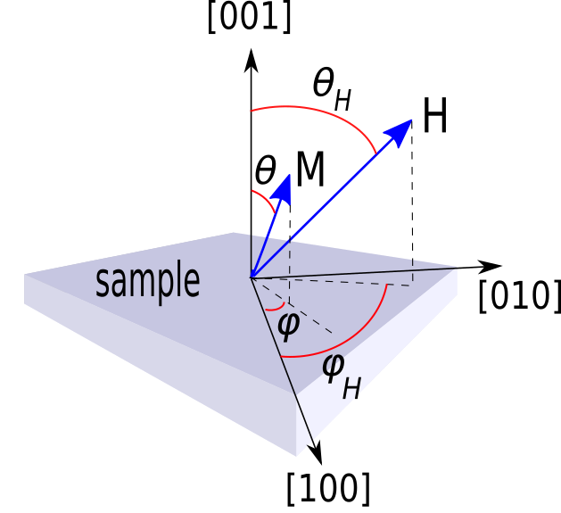
Figure 1: The geometry of the FMR experiment. The orientation of the applied magnetic field ${\mathbf{H}}$ is usually described in the coordinate system attached to the crystallographical axes of the sample. The field direction is represented by angles $\vartheta_{H}$ and $\varphi_{H}$ and equilibrium direction of the sample magnetization ${\mathbf{M}}$ is represented by angles $\vartheta$ and $\varphi$.

What does one measure while performing FMR experiment? — The most simple answer is that the spatial distribution of resonance field $\mathbf{H}_{r}$ is measured, i.e., its dependence on angles $\vartheta_{H}$ and $\varphi_{H}$, see Fig. 1. However, let us consider two possible ways of performing the FMR experiment. First, while fixing a frequency $\omega$ of an alternating microwave field one measures the dependence of the static magnetic field $\mathbf{H}_{r}$ on angles $\vartheta_{H}$ and $\varphi_{H}$ at resonance, and the second — a static magnetic field is fixed and one changes the frequency of microwave field to find a frequency at which the precession of the magnetic moment of the sample occurs. The resonance condition, for both measurement methods, is given by the following Smit-Beljers equation [Smit and Beljers, 1955; Artman, 1957; Baselgia et al., 1988; Morrish, ]

$$\bigg{(}\frac{\hbar\omega}{g\mu_{B}}\bigg{)}^{2}=\frac{1}{\mbox{sin}^{2}\vartheta}(f_{\vartheta\vartheta}f_{\phi\phi}-f^{2}_{\vartheta\phi}),$$ (1)

where $f$ is free energy of the sample divided by its saturation magnetization $M$, i.e., free energy is expressed in terms of real (Zeeman term) and fictitious (demagnetizing and anisotropy terms) fields. $f_{\vartheta\phi}=\frac{\partial f}{\partial\vartheta}\frac{\partial f}{\partial\varphi}$, $g$ is the spectroscopic splitting factor, $\mu_{B}$ – the Bohr magneton and $\hbar$ – the Planck constant.

Let us recall, that the Gaussian curvature of the surface $\mathcal{S}(\vartheta,\varphi)$ at one of its points, being the product of two principal curvatures $\kappa_{1}$ and $\kappa_{2}$, is the determinant of the Hessian matrix calculated at this point. One obtains in spherical coordinates

$$\kappa_{1}\kappa_{2}=\mbox{det}\begin{bmatrix}\frac{\partial^{2}\mathcal{S}}{\partial\vartheta^{2}}&\frac{1}{\sin\vartheta}\frac{\partial^{2}\mathcal{S}}{\partial\mathcal{S}\vartheta\partial\varphi}-\frac{\cot\vartheta}{\sin\vartheta}\frac{\partial\mathcal{S}}{\partial\varphi}\\ \frac{1}{\sin\vartheta}\frac{\partial^{2}\mathcal{S}}{\partial\varphi\partial\vartheta}-\frac{\cot\vartheta}{\sin\vartheta}\frac{\partial\mathcal{S}}{\partial\varphi}&\frac{1}{\sin^{2}\vartheta}\frac{\partial^{2}\mathcal{S}}{\partial\varphi^{2}}+\cot\vartheta\frac{\partial\mathcal{S}}{\partial\vartheta}\end{bmatrix}.$$ (2)

Let us now assume that we are interested in the curvature of the the free energy landscape of the sample at resonance and put $\mathcal{S}=f$ in Eq. (2). Remembering that $\bf M$ precesses around its eqilibrium position, that is, the equations

$$\frac{\partial f}{\partial\vartheta}=0,\,\,\,\frac{\partial f}{\partial\varphi}=0$$ (3)

are satisfied, we arrive at Eq. (1) if we interpret $\big{(}\frac{\hbar\omega}{g\mu_{B}}\big{)}^{2}$ as a Gaussian curvature of the spatial distribution of free energy.

Returning to the two ways of measuring the resonance field we see, that by fixing a static field and subsequent measuring the frequency $\omega$ of a microwave field for different angles at resonance, we see directly a spatial distribution of the curvature of the free energy landscape. If, however, we set the microwave field, and then by changing the static field we hit the resonance ($\mathbf{H}_{r}$) for different angles $\vartheta_{H}$ and $\varphi_{H}$ then we will maintain a constant Gaussian curvature of the energy landscape during the measurement.

The answer to the question posed at the beginning of this section is, that while performing a typical FMR experiment by fixed $\omega$, we measure such a field $\mathbf{H}_{r}$ at which the Gaussian curvature $\kappa_{1}\kappa_{2}$ of the free energy landscape is constant, i.e., does not depend on $\vartheta_{H}$ and $\varphi_{H}$. As we shall see, this observation will not only allow finding contributions from various types of anisotropy to the free energy but also will enable the determining of saturation magnetization of the sample.

What determines the spatial distribution of the Gaussian curvature of the free energy at resonance? — Assume that the free energy density $F(\vartheta_{H},\varphi_{H})$ of a ferromagnet placed in a magnetic field, expressed in terms of magnetic fields, is given by

$$\begin{split}\frac{F(\vartheta_{H},\varphi_{H})}{M}=f(\vartheta_{H},\varphi_{H})=-H\sum_{\alpha}n_{\alpha}n^{H}_{\alpha}\\ +M\sum_{\alpha,\beta}\mathcal{N}_{\alpha\beta}n_{\alpha}n_{\beta}+\frac{1}{2}H_{c}\sum_{\alpha\neq\beta}n^{2}_{\alpha}n^{2}_{\beta}.\end{split}$$ (4)

${\alpha,\beta}=x,y,z$. The first term on the right-hand side of Eq. (4) is the Zeeman energy, the second term is the demagnetizing energy, with $\mathcal{N}_{\alpha\beta}$ being the demagnetization tensor. The last term describes the energy related to cubic magnetocrystalline anisotropy. The components of vectors $n_{\alpha}^{H}=\mathbf{H}/H$ and $n_{\alpha}=\mathbf{M}/M$ are defined as usuall, see e.g., Eqs. (3a) and (3b) in Ref. [Tomczak and Puszkarski, 2018] and Fig. 1. Note that with fulfilled relations (3), the free energy of a sample with a specific geometry and saturation magnetization in a magnetic field does not depend on angles $\vartheta,\varphi$ explicitly.

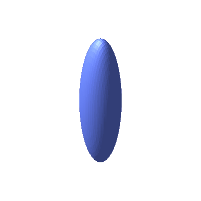
(a)

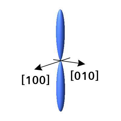
(b)

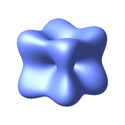
(c)

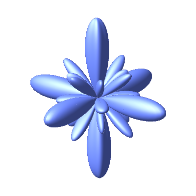
(d)

Figure 2: Terms in Eq. (4) representing fictitious magnetic fields and their Gaussian curvatures (a) $M\sum_{\alpha,\beta}\mathcal{N}_{\alpha\beta}n_{\alpha}n_{\beta}$ (ellipsoid) (b) its curvature (c) $\frac{1}{2}H_{c}\sum_{\alpha\neq\beta}n^{2}_{\alpha}n^{2}_{\beta}$ (d) its curvature.

Each component of Eq. (4) describes a spatially varying magnetic field with a certain curvature. For example the spatial dependencies of the first two terms and their curvatures are shown in Fig. 2. Surface (a) - ellipsoid - represents the fictitious demagnetizing field for the sample oriented along axes [100], [010] and [001]. Its curvature is shown in Fig. 2b. Note that it is non-zero in the (001) plane, although this is not visible due to the used scale. The surface (c) represents the first order cubic magnetocrystalline fictitious field and in Fig. 2d is shown its curvature. The curvature of the Zeeman term in Eq. (4) depends on the static magnetic field and can be changed during the measurement while the curvatures associated with the fictitious demagnetizing and cubic anisotropy fields remain constant during the measurement.

How to find saturation magnetization and anisotropy fields numerically? — During the FMR experiment the total Gaussian curvature of the free energy remains constant: contributions of curvatures from various fictitious magnetic fields (anisotropy, demagnetizing), related to the sample itself, are compensated by the curvature of the Zeeman term. To find numerically values of those fields, $g$-factor and saturation magnetization we apply a procedure to some extent reverse to the measurement: for a given set of measured $H_{r}(\vartheta_{H},\varphi_{H})$ data, collected in a single experiment, the constant $g$, $M$ and anisotropy and demagnetizing fields should be chosen so that Eq. (1) should be met for all measured static resonance fields $H_{r}(\vartheta_{H},\varphi_{H})$. It means, that minimizing an appropriate objective function, which measures the deviation from the constant curvature with respect to unknown anisotropy fields, $g$ and $M$ lets us find them. This procedure is described in detail in Ref. [Tomczak and Puszkarski, 2018]. The key point for finding saturation magnetization is that its change leads to the change of the curvature of the demagnetizing field. But to ensure that the determined magnetization value is unambiguous, the constraint $\mathcal{N}_{x}+\mathcal{N}_{y}+\mathcal{N}_{z}=1$ should be met during the minimization procedure.

To carry out the minimization procedure, it is necessary to know the functional form of free energy. Usually one assumes its specific form taking into account the symmetry of the system — free energy should be invariant under relevant symmetry transformations. Then it is possible to expand it into basis functions (orthogonal or non-orthogonal) with the same symmetry. Typically this expansion is limited to some low-order terms of systematically decreasing basis functions. It should be remembered, however, that in the case of examination of curvature, the higher-order basis functions may give greater contributions to total curvature of free energy than the lower-order ones.

Numerical example I: Saturation magnetization of bulk magnetite — Bickford [Bickford, 1950] measured the resonance fields for disk-shaped samples of magnetite cut in (100) and (110) planes. The results of his measurements are shown as blue squares in Figs 3a and 3b, respectively. Each sample was oriented differently with respect to the crystallographic planes and thus it has different demagnetization tensor. We will assume, however, that both types of samples have the same $g$-factor and the same saturation magnetization. The demagnetizing tensor is assumed to be diagonal for samples cut in (100) plane

$$\mathcal{N}_{(100)}=\begin{bmatrix}\mathcal{N}_{x}&0&0\\ 0&\mathcal{N}_{y}&0\\ 0&0&\mathcal{N}_{z}\end{bmatrix}.$$ (5)

The curvature of free energy distribution, given by Eq. (1), depends now on six parameters which we denote collectively by the vector ${\mathbf{h}_{B}}=(g,M,\mathcal{N}_{x},\mathcal{N}_{y},\mathcal{N}_{z},H_{c}).$ Using the procedure described in Ref. [Tomczak and Puszkarski, 2018], we get the following coordinates of the vector ${\mathbf{h}_{B}}$

$$\begin{split}{\mathbf{h}_{B}}=(2.220(88),5.906(150),0.2216(267),0.2212(268),\\ 0.5572(535),-0.2392(95)).\end{split}$$ (6)

Both, $M$ and $H_{c}$ are given in kOe. The errors (in brackets) refer to the last significant digits and were calculated assuming that the measurement errors are subject to normal distribution. Having determined the vector ${\mathbf{h}_{B}}$, we solve Eq. (4) numerically with respect to ${\mathbf{H}}_{\mathrm{r}}$ and get the resonance field dependence on the $\vartheta_{H}$ angle (black line in Fig. 3a). To consider measurements of samples cut in the plane (110) let us rotate the coordinate system in such a way, that the $z$ axis is perpendicular to the (110) plane. The demagnetizing tensor is given by

$$\mathcal{N}_{(110)}\!=\!\begin{bmatrix}\frac{1}{4}(\mathcal{N}_{xy}+2\mathcal{N}_{z})&\frac{1}{4}(\mathcal{N}_{xy}-2\mathcal{N}_{z})&\frac{\sqrt{2}}{4}(\mathcal{N}_{y}-\mathcal{N}_{x})\\ \frac{1}{4}(\mathcal{N}_{xy}-2\mathcal{N}_{z})&\frac{1}{4}(\mathcal{N}_{xy}+2\mathcal{N}_{z})&\frac{\sqrt{2}}{4}(\mathcal{N}_{y}-\mathcal{N}_{x})\\ \frac{\sqrt{2}}{4}(\mathcal{N}_{y}-\mathcal{N}_{x})&\frac{\sqrt{2}}{4}(\mathcal{N}_{y}-\mathcal{N}_{x})&\frac{1}{2}\mathcal{N}_{xy}\end{bmatrix}\!\!,$$ (7)

$\mathcal{N}_{xy}$ stands for $\mathcal{N}_{x}+\mathcal{N}_{y}$. Solving again Eq. (4) for such a tensor $\mathcal{N}_{(110)}$, we reach the dependence of ${\mathbf{H}}_{r}(\vartheta_{H})$ shown in Fig. 3b. In Table 1 the relevant anisotropy constants found by Bickford are presented compared with those obtained in the way as described in the text.

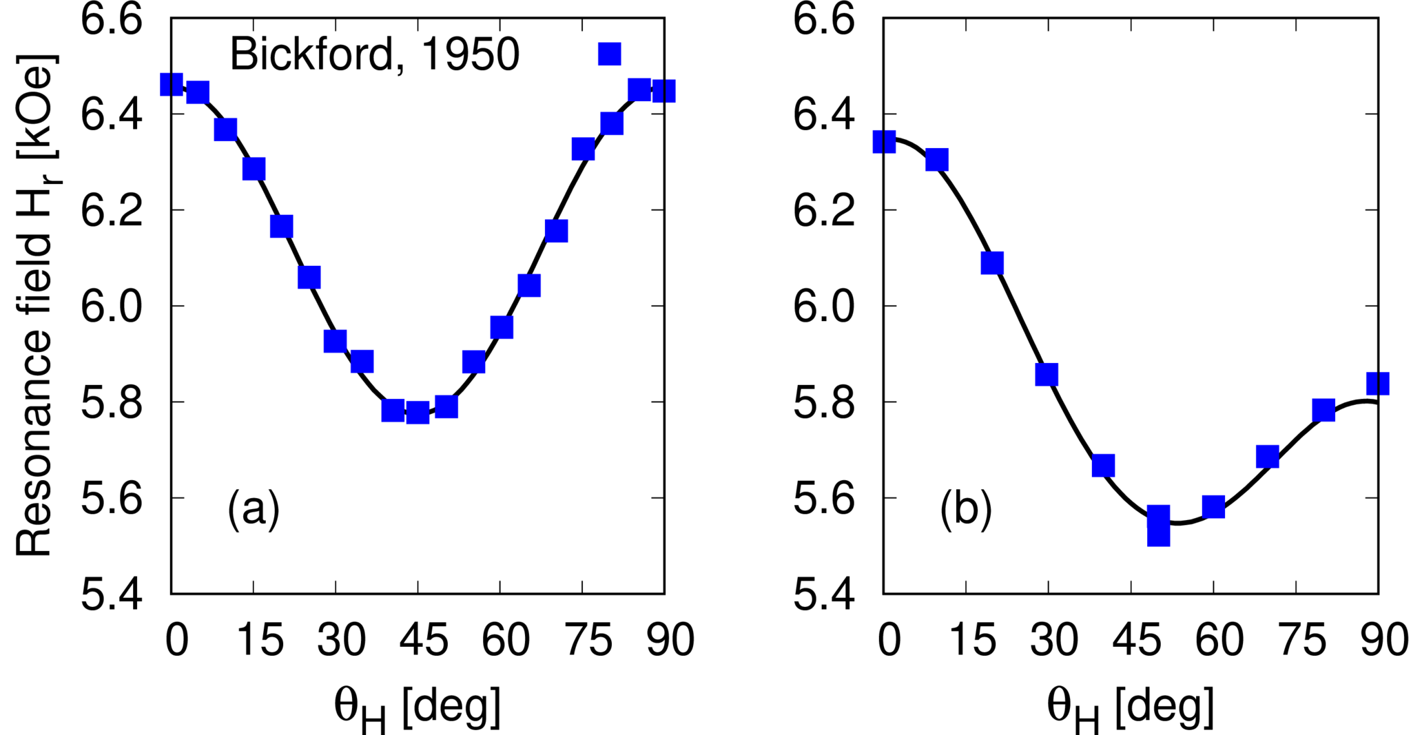
Figure 3: Resonance field versus out-of-plane angle $\vartheta_{H}$ for bulk magnetite for samples cut in (100) – (a) and (110) planes – (b). Squares - Bickford’s measurements [Bickford, 1950], black line - solution of Smit-Beljers equation for the vector ${\mathbf{h}_{B}}$ given by Eq. (6). Figs (a) and (b) correspond to Figs 3 and 4 in Ref. [Bickford, 1950], respectively.

To summarize this example, let us stress two things. First, we observe a fairly large statistical errors that are the result of the scattering of original measurements reported in Ref. [Bickford, 1950]. Second, in fact, the Bickford’s samples had the shapes of a circular flattened disks, since in (100) geometry $\mathcal{N}{x}\approx\mathcal{N}{y}\neq\mathcal{N}{z}$.

Table 1: Comparison of $g$-factor, saturation magnetization $M$ and cubic anisotropy constant $K_{c}$ values found by Bickford [Bickford, 1950]with those obtained by the method described in the text. The errors (in brackets) refer to the last significant digits.

	$g$	$M$ [kA/m]	$K_{c}$ [kJ/m3]
	2.220(88)	470(12)	-14.12(92)
Ref. [Bickford, 1950]	2.07	472	-11

Numerical example II: Saturation magnetization of the (Ga,Mn)As thin film — In Ref. [Tomczak and Puszkarski, 2018] we showed, analyzing Liu’s measurements [Liu et al., 2007] of resonance fields for the weak ferromagnet (Ga,Mn)As, that in order to properly describe the free energy spatial distribution at resonance, one should expand it up to the fourth order with respect to cubic anisotropy fields. Here we add to this expansion demagnetizing fields, and, since the sample was oriented along crystallographical axes of (Ga,Mn)As we use a diagonal form od the demagnetizing tensor. The vector ${\mathbf{h}_{L}}$ depends now on eleven parameters

$${\mathbf{h}_{L}}\equiv(g,M,\mathcal{N}_{x},\mathcal{N}_{y},\mathcal{N}_{z},H_{c1},...,H_{c4},H_{[001]},H_{[110]}).$$ (8)

Anisotropy fields are denoted like in Ref. [Tomczak and Puszkarski, 2018]. The minimization procedure leads to (fields are given in Oe)

$$\begin{split}{\mathbf{h}_{L}}=(1.984(3),383.5(2.2),0.08104(90),0.06796(95),\\ 0.8510(20),76.86(0.42),-539.5(10.0),42.86(0.92),\\ 1412(70),4213(24),68.08(0.64)).\end{split}$$ (9)

The numerical solutions of Eq. (1) for such an ${\mathbf{h}_{L}}$ vector is shown in Fig. 4. They are equivalent to those obtained in Ref. [Tomczak and Puszkarski, 2018] but now the use of the demagnetizing fields made it possible to determine saturation magnetization $M=30.52(0.18)$ [emu/cm³].

Figure 4: Resonance field versus out-of-plane angle $\vartheta_{H}$ (a) and versus in-plane angle $\varphi_{H}$ (b) for (Ga,Mn)As film. Squares - Liu measurements [Liu et al., 2007], black line - solution of Smit-Beljers equation for the vector ${\mathbf{h}_{L}}$ (Eq. 9). Figs (a) ad (b) correspond to Figs 5 and 6 in Ref. [Liu et al., 2007], respectively.

Numerical example III: Saturation magnetization of the YIG ultrathin thin film — The measurements of the resonance field of the 9.8 nm thin film are taken from Ref. [Wang et al., 2014] and shown in Figs 5a and 5b, respectively, as blue squares. To determine the anisotropy fields let us assume that the free energy is given by Eq. (1) from Ref. [Wang et al., 2014] and that the demagnetizing fields, as in the (Ga,Mn)As case, are calculated using a diagonal demagnetizing tensor. Then the vector ${\mathbf{h}_{H}}$ depends on nine parameters

$$\begin{split}{\mathbf{h}_{H}}=(g,M,\mathcal{N}_{x},\mathcal{N}_{y},\mathcal{N}_{z},H_{2\perp},H_{4\perp},H_{2\parallel},H_{4\parallel}).\end{split}$$ (10)

Factor $g$ = 2 for YIG [Stancil, ], while saturation magnetization $M$ = 1851 [Oe] was determined for this sample using a vibrating sample magnetometer [Wang et al., 2014].

The components of the vector ${\mathbf{h}_{H}}$ corresponding to the constant curvature of free energy, i.e., for the sample at resonance, are collected in Table 2 for four cases. In the first case, we take $g$ and $M$ values as measured experimentally and find remaining ones. In the second case we fix only experimental value of $M$, in the third case - only value of $g$, and finally, we treat both $g$ and $M$ as unknown (last row of in Table 2). In the last column of Table 2 the error function $E_{RMS}^{1}({\mathbf{h}_{H}})$ is given, as defined in Ref. [Tomczak and Puszkarski, 2018]. Its value informs us about the quality of the prediction of new experimental results of resonance fields calculated from a given free energy formula with specific values (row of Table 2) of anisotropy fields. We see that analysis of FMR measurements of the YIG ultrathin film gives worse results when we treat measured $g$ and $M$ values as known. This points out that the form of free energy used for this analysis is not chosen optimally, because it was not possible to reproduce the experimental values $g$ and $M$ with satisfactory accuracy. Thus the presented method may also serve as a test for the correctness of the assumed free energy form. Note also, that although the investigated film was ultrathin, we obtained non-zero values of the demagnetization fields in the (001) plane. The dependencies of resonance fields on angles $\vartheta_{H}$ and $\varphi_{H}$ are shown, for ${\mathbf{h}_{H}}$ from the first row of Table 2, in Fig. 5.

Table 2: Comparison of $g$-factor, saturation magnetization $M$ and and anisotropy field values found in Ref. [Wang et al., 2014] with those obtained by the method described in the text. The errors (in brackets) refer to the last significant digits.

	$g$	$M$[Oe]	$\mathcal{N}_{x}$	$\mathcal{N}_{y}$	$\mathcal{N}_{z}$	$H_{2\perp}$[Oe]	$H_{4\perp}$[Oe]	$H_{2\parallel}$[Oe]	$H_{4\parallel}$[Oe]	$E_{RMS}^{1}({\mathbf{h}_{H}})$
	2.000	1851	0.08429(10)	0.08721(11)	0.8285(10)	-497.7(2.0)	372.3(1.1)	62.23(0.27)	49.02(0.22)	0.815
	2.014(1)	1851${}^{\textrm{b}}$	0.08795(17)	0.08985(10)	0.8222(15)	-466.5(1.5)	276.9(0.9)	61.83(0.23)	47.27(0.18)	0.691
	2.000${}^{\textrm{a}}$	1800(11)	0.08102(15)	0.08408(11)	0.8349(16)	-538.9(1.7)	372.6(1.0)	62.16(0.11)	49.05(0.16)	0.815
	2.013(1)	1772(12)	0.08263(8)	0.08467(13)	0.8327(13)	-526.2(1.6)	277.5(0.9)	61.82(0.09)	47.42(0.18)	0.691
Ref. [Wang et al., 2014]		1851(37)				-1253(25)		60.4(1.2)	42.0(1.2)

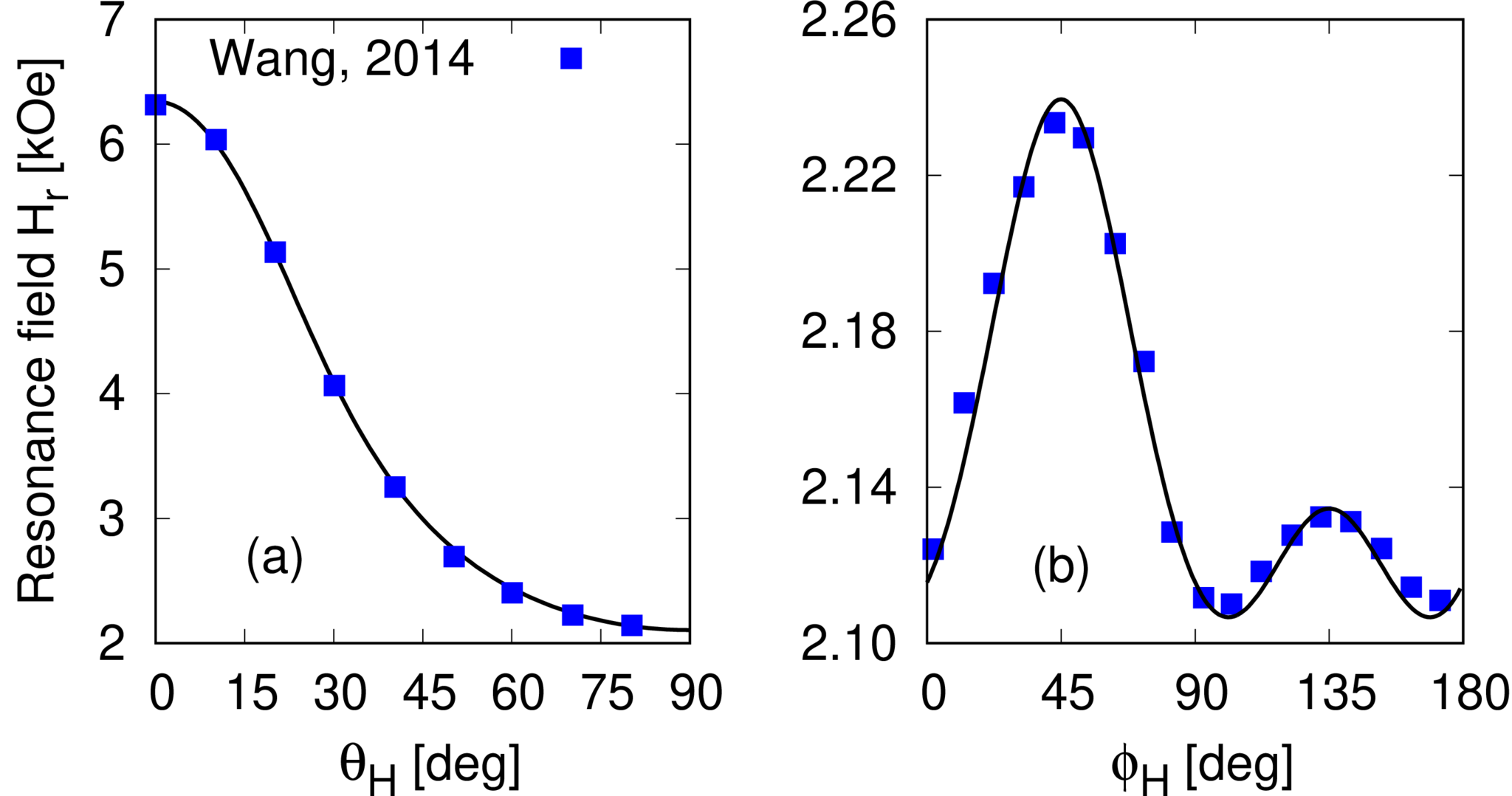
Figure 5: Resonance field for 9.8 nm ultrathin YIG film versus out-of-plane angle $\vartheta_{H}$ (a) and in-plane angle $\phi_{H}$ (b). Squares - Wang’s measurements [Wang et al., 2014], black line - solution of Smit-Beljers equation for the vector ${\mathbf{h}_{H}}$ given by Eq. (10). Figs (a) and (b) correspond to Figs 2(b) and 2(c) in Ref. [Wang et al., 2014], respectively .

Conclusion — We presented in this article one more approach to the interpretation of the classical FMR experimental data. It is based on the analysis of the curvature of the spatial dependence of free energy of the sample at resonance and makes it possible, after assuming the functional form of free energy, to determine (with an accuracy of 0.5-4% in the presented numerical examples) the sample saturation magnetization and, consequently, the spatial dependence of magnetocrystalline energy stored in the sample in a single FMR experiment. The method presented here can also be a test for the correctness of the assumed form of free energy of the sample at resonance. This may be important for people working in the field of magnetic resonance.

Acknowledgment — This study is a part of the project financed by Narodowe Centrum Nauki (National Science Centre of Poland) No. DEC-2013/08/M/ST3/00967. Numerical calculations were performed at Poznań Supercomputing and Networking Center under Grant No. 284.

References

- Farle (1998) M. Farle, Reports on Progress in Physics 61, 755 (1998).
- Tomczak and Puszkarski (2018) P. Tomczak and H. Puszkarski, Phys. Rev. B 98, 144415 (2018).
- Smit and Beljers (1955) J. Smit and H. G. Beljers, Philips Res. Rep. 10, 113 (1955).
- Artman (1957) J. O. Artman, Phys. Rev. 105, 74 (1957).
- Baselgia et al. (1988) L. Baselgia, M. Warden, F. Waldner, S. L. Hutton, J. E. Drumheller, Y. Q. He, P. E. Wigen, and M. Maryško, Phys. Rev. B 38, 2237 (1988).
- (6) A. Morrish, The Physical Principles of Magnetism (Wiley-IEEE Press, 2001).
- Bickford (1950) L. R. Bickford, Phys. Rev. 78, 449 (1950).
- Liu et al. (2007) X. Liu, Y. Y. Zhou, and J. K. Furdyna, Phys. Rev. B 75, 195220 (2007).
- Wang et al. (2014) H. Wang, C. Du, P. C. Hammel, and F. Yang, Phys. Rev. B 89, 134404 (2014).
- (10) D. Stancil, A. Prabhakar, Spin Waves. Theory and Applications (Springer, 2009).