A rational approximation method for the nonlinear eigenvalue problem

Abstract

This paper presents a method for computing eigenvalues and eigenvectors for some types of nonlinear eigenvalue problems. The main idea is to approximate the functions involved in the eigenvalue problem by rational functions and then apply a form of linearization. Eigenpairs of the expanded form of this linearization are not extracted directly. Instead, its structure is exploited to develop a scheme that allows to extract all eigenvalues in a certain region of the complex plane by solving an eigenvalue problem of much smaller dimension. Because of its simple implementation and the ability to work efficiently in large dimensions, the presented method is appealing when solving challenging engineering problems. A few theoretical results are established to explain why the new approach works and numerical experiments are presented to validate the proposed algorithm.

1 Background and introduction

Consider a non-empty open set $\Omega\subset\mathbb{C}$ and a matrix-valued function $T(z):\Omega\rightarrow\mathbb{C}^{n\times n}$ that is analytic on $\Omega$, i.e., each component of $T(z)$ is an analytic function of $z$. The nonlinear eigenvalue problem (NLEVP) consists of finding $\lambda\ \in\Omega$ and a nonzero vector $u\ \in\ \mathbb{C}^{n}$ such that:

$${}T(\lambda)u=0.$$ (1)

We call $\lambda$ an eigenvalue of $T(\cdot)$ and $u$ the associated eigenvector. Problems of this type arise in numerous applications, including in the analysis of vibration of rails under excitation from fast trains [34, 3], in the optimization of acoustic emissions of high speed trains [45], in electronic structure calculations of quantum dots [32, 69], and in the study of photonic resonators at the nanoscale [15, 68]. As a result, these problems have been extensively studied in the literature [65, 47, 70, 46, 29] and a plethora of specialized methods were developed for different types of structures of $T(z)$, see e.g. [65] for quadratic or [46, 44] for polynomial eigenvalue problems.

The first type of nonlinear eigenvalue problems that were studied were polynomial eigenvalue problems (PEPs) in which $T(z)$ is a polynomial of small degree in $z$, with matrix coefficients. These problems can be easily converted into an equivalent (same eigenvalues) generalized eigenvalue problem via linearization. The resulting, larger problem, is then solved by standard techniques [27]. Linearization-based approaches for solving polynomial eigenvalue problems have been extensively studied, see, e.g., [26, 47].

This work focuses on computing the eigenvalues of general nonlinear eigenvalue problems, i.e., those for which $T(z)$ is not a polynomial. The goal is to compute all eigenvalues located inside a closed contour $\Gamma$ of the complex plane. State-of-the-art numerical methods for general nonlinear eigenvalue problems include Newton-type methods, e.g., [36, 38, 67, 54, 51, 37, 57, 58, 12, 35], techniques based on contour integration [4, 14, 13, 20, 71, 25], and methods based on polynomial and rational approximations of $T(z)$, e.g.,  [47, 45].

The method proposed in this paper belongs to the last of the three categories listed above and it relies specifically on rational approximations obtained from the Cauchy integral formula. Among methods that exploit contour integrals, Beyn’s method [13] figures prominently and is currently the best known. Given a matrix $Q$ which contains a set of $k$ vectors, e.g., chosen randomly, Beyn’s method exploits the relation between the following matrices, called $p$-th (order) moments,

$$S_{p}=\frac{1}{2\pi\imath}\int\limits_{\Gamma}z^{p}T(z)^{-1}Q\ dz,\quad p=0,1,2,\ldots$$ (2)

By Keldysh’s theorem, under certain conditions, $T(z)^{-1}$ can be written locally as $T(z)^{-1}=U(zI-\Lambda)^{-1}W^{H}+R(z)$, where $R(z)$ is analytic and therefore:

$$S_{0} = \frac{1}{2\pi\imath}\int\limits_{\Gamma}T(z)^{-1}Q\ dz=UW^{*}Q\ \in\mathbb{C}^{n\times k},$$

$$S_{1} = \frac{1}{2\pi\imath}\int\limits_{\Gamma}zT(z)^{-1}Q\ dz=U\Lambda W^{*}Q\ \in\mathbb{C}^{n\times k}.$$ (3)

The idea then is to exploit the relation between the two matrices on the right-hand sides of the above equations, to extract $\Lambda$. For this purpose, the algorithm relies on the singular value decomposition (SVD).

Different interpretations of the method just sketched have been exploited. Thus, the article [7] made a link between Beyn’s method and rational filters which are exploited to “filter” (extract) the approximate invariant subspace corresponding to the eigenvalues $\lambda_{i},i=1,\ldots,n_{\Gamma},$ located inside $\Gamma$. This led to a study of general filter functions of the form

$$\sum\limits_{j=0}^{N-1}\frac{\omega_{j}z_{j}^{p}}{z_{j}-z},$$ (4)

for solving NLEVPs in [7] and in  [6]. The filtering nature of contour integral methods is also explored in the Nonlinear FEAST algorithm [25]. In this context, we also mention the interesting work by Embree et al. [22] who make the connection with transfer functions of dynamics in system theory.

The method proposed in this paper takes a general NLEVP, approximates it with a rational eigenvalue problem and then solves this rational problem by a form of linearization. This general approach is not new and the following is a short, albeit incomplete, overview of this class of techniques. In the rational Krylov-based approach known as Newton rational Krylov proposed in [9], the matrix-valued function $T(z)$ is first approximated by a low-degree Hermite interpolating polynomial in Newton form. The resulting generalized eigenvalue problem is then solved by a rational Krylov method, with the interpolations points taken as shifts. This leads to a flexible approach that can easily incorporate information from the most recent iterations, take advantage of the underlying structure of the problem and simultaneously find several eigenvalues of interest. To improve convergence, the Newton rational Krylov method was generalized from polynomial to linear rational interpolation, resulting in an algorithm called fully rational Krylov method for NLEVPs, commonly refereed as NLEIGS, see [28]. Of particular interest is the dynamic NLEIGS variant which utilizes the rational Newton expansion and the companion-like strong linearizations to dynamically add interpolation nodes and poles to extend the matrix pencils, and to merge the construction of the rational approximation with the application of the rational Krylov method.

When solving large-scale nonlinear eigenvalue problems, it is essential to exploit the structure of the linearized problem in order to overcome the large memory and computational costs. This is the primary goal of compact rational Krylov (CORK) framework proposed in [10]. In this general framework it is assumed that the approximation of $T(z)$, whether polynomial or rational, is put in the form $\widetilde{T}(z)=\sum_{i=0}^{d-1}(A_{i}-\lambda B_{i})f_{i}(z),$ with the scalar functions $f_{i}(z)$ satisfying a linear recurrence relation $M_{d}\textbf{f}_{d}=zN_{d}\textbf{f}_{d}(z),$ where $\textbf{f}_{d}=\big{[}f_{0}(z),f_{1}(z),\ldots,f_{d-1}(z)\big{]}^{T}$ and $M_{d},N_{d}\in\mathbb{C}^{(d-1)\times d}$. Then the associated companion linearization, often referred as CORK linearization, turns out to have a particularly interesting structure, namely: $\textbf{L}(z)=\textbf{A}-z\textbf{B}$, where

$$\textbf{A}=\left[\begin{array}[]{cccc}A_{0}&A_{1}&\cdots&A_{d-1}\\ \hline\cr\lx@intercol\hfil M_{d}\otimes I_{n}\hfil\lx@intercol\end{array}\right],\qquad\textbf{B}=\left[\begin{array}[]{cccc}B_{0}&B_{1}&\cdots&B_{d-1}\\ \hline\cr\lx@intercol\hfil N_{d}\otimes I_{n}\hfil\lx@intercol\end{array}\right].$$ (5)

If $\widetilde{T}(z)$ is a matrix polynomial, the pencil (5) is the classical companion-like linearization [26]. The Kronecker structure of the CORK pencil (5) allows to efficiently solve the associated generalized eigenvalue problem using a rational Krylov method [55, 56]. With a compact representation $v=(I\otimes Q)u$ (Arnoldi decomposition [61]) of the right Krylov vectors $v$, with $Q$ having orthonormal columns and $u$ being of much smaller dimension than $v$, CORK can be characterized as a two-step procedure similar to the two-level orthogonal Arnoldi (TOAR) [41]. The orthogonalization step involving vectors of original problem size $n$ followed by a standard rational Krylov step on a projected matrix pencil, significantly lower the overall memory and computational costs of the CORK algorithm. Moreover, both the implicit restarting procedure and utilizing low-rank structure of coefficient matrices $A_{i}$ and $B_{i}$ make CORK method highly competitive when it comes to solving efficiently and reliably challenging nonlinear eigenvalue problems [8]. Extensions and refinements of the CORK framework were proposed in [39, 53, 16, 60, 39, 40, 50].

The method we propose is in the same family as those described above but there are distinctions. First, we rely entirely on the Cauchy integral formula to approximate $T(z)$ directly. As will be seen in Section 2, the resulting approximation is a rational function which includes simple terms of the form $B_{i}/(z-\sigma_{i})$. As it was already made clear above, an essential part of the methods for solving rational eigenvalue problems, is exploiting a good linearization. A large volume of work has been devoted to linearizations both from a practical and from a theoretical viewpoint [1, 2, 18, 17, 23, 24, 26, 31, 46, 42, 43, 45, 62, 63, 64]. We propose a simple and natural linearization technique which lends itself to efficient calculations.

The method we propose in this paper exploits a projection technique that employs vectors of length $n$, the size of the original problem. A slight modification of the method was recently used to solve a rather challenging nonlinear eigenvalue problem that arises from applying the Boundary Element Method in acoustics [21]. The experiments proposed at the end of the paper are presented primarily for illustrating certain characteristics of the method including its versatility and ease of use.

2 A rational approximation approach for NLEVPs

Following Kressner [35], we limit ourselves to problems in which:

$$T(z)=f_{0}(z)A_{0}+f_{1}(z)A_{1}+f_{2}(z)A_{2}+\ldots+f_{p}(z)A_{p},$$ (6)

with holomorphic functions $f_{0},\ldots,f_{p}:\Omega\rightarrow\mathbb{C}$ and constant coefficient matrices $A_{0},\ldots,A_{p}$. In what follows, we will call $\Gamma$ the boundary of $\Omega$. Since $T\in H(\Omega,\mathbb{C})$, it can always be written in the form (6) with at most $p=n^{2}$ terms. Note also that this representation is not unique. Furthermore, it is very common in practice to have $f_{0}(z)=1$ and $f_{1}(z)=z$, so instead of the above we will assume the form:

$$T(z)=-B_{0}+zA_{0}+f_{1}(z)A_{1}+\ldots+f_{p}(z)A_{p}.$$ (7)

As it turns out many of the nonlinear eigenvalue problems encountered in applications are set in this form. We are interested in all eigenvalues that are located in a region of the complex plane enclosed by curve $\Gamma$.

The main assumption we make is that each of the holomorphic functions $f_{j}:\Omega\rightarrow\mathbb{C}$ in representation (7) is well approximated by a rational function of the form:

$$f_{j}(z)\approx\sum_{i=1}^{m}\frac{\alpha_{ij}}{z-\sigma_{i}}.$$ (8)

Note that the set of $m$ poles $\sigma_{i}$’s is the same for all of the functions. This setting comes from a Cauchy integral representation of each function inside a region limited by a contour $\Gamma$:

$$f_{j}(z)=-\frac{1}{2i\pi}\int_{\Gamma}\frac{f_{j}(t)}{z-t}\ dt,\quad\quad z\in\Omega.$$ (9)

Using numerical quadrature, (9) is then approximated into (8), where the $\sigma_{i}$’s are quadrature points located on the contour $\Gamma$. Substituting (8) into (7) yields the following approximation $\widetilde{T}(z)$ of $T(z)$:

$$\widetilde{T}(z) =-B_{0}+zA_{0}+\sum_{j=1}^{p}\sum_{i=1}^{m}\frac{\alpha_{ij}}{z-\sigma_{i}}A_{j}=-B_{0}+zA_{0}+\sum_{i=1}^{m}\ \frac{\sum_{j=0}^{p}\alpha_{ij}A_{j}}{z-\sigma_{i}}$$

$$\equiv\ -B_{0}+zA_{0}+\sum_{i=1}^{m}\ \frac{B_{i}}{z-\sigma_{i}},$$ (10)

where we have set

$$B_{i}=\sum_{j=0}^{p}\alpha_{ij}A_{j},\qquad i=1,\ldots,m.$$ (11)

Given the approximation $\widetilde{T}(z)$ of $T(z)$ shown in (10), the problem we need to solve can be written as follows:

$$\Big{(}-B_{0}+\lambda A_{0}+\sum_{i=1}^{m}\ \frac{B_{i}}{\lambda-\sigma_{i}}\Big{)}u=0\ .$$ (12)

We will often refer to this problem as a surrogate for problem (1). It will be seen that if each of the functions $f_{j}$ is well approximated then this surrogate problem will provide good approximations to eigenvalues of $T(z)$ located inside the contour but that are not close to the poles.

For a given complex number $z$, and a given vector $u$, we define

$$v_{i}=\frac{u}{\sigma_{i}-z},\qquad i=1,\ldots,m.$$ (13)

Then we can write

$$\widetilde{T}(z)u =\Big{(}-B_{0}+zA_{0}+\sum_{i=1}^{m}\frac{B_{i}}{z-\sigma_{i}}\Big{)}u$$ (14)

$$=(-B_{0}+zA_{0})u-\sum_{i=1}^{m}B_{i}v_{i},$$ (15)

which can be expressed in block form as follows:

$$\begin{bmatrix}(z-\sigma_{1})I&&&&I\\ &(z-\sigma_{2})I&&&I\\ &&\ddots&&\vdots\\ &&&(z-\sigma_{m})I&I\\ -B_{1}&-B_{2}&\ldots&-B_{m}&zA_{0}-B_{0}\end{bmatrix}w=0,\quad w=\begin{bmatrix}v_{1}\\ v_{2}\\ \vdots\\ v_{m}\\ u\end{bmatrix}\ .$$ (16)

Since (16) is of the form $(z{\cal M}-{\cal A})w=0$, solutions of the surrogate eigenvalue problem $\widetilde{T}(\lambda)u=0$ can be obtained by solving the linear eigenvalue problem

$${\cal A}w=\lambda{\cal M}w,$$ (17)

with

$${\cal M}=\begin{bmatrix}I&&&&\\ &I&&&\\ &&\ddots&&\\ &&&\ddots&\\ &&&&A_{0}\end{bmatrix},\qquad{\cal A}=\begin{bmatrix}\sigma_{1}I&&&&-I\\ &\sigma_{2}I&&&-I\\ &&\ddots&&\vdots\\ &&&\sigma_{m}I&-I\\ B_{1}&B_{2}&\ldots&B_{m}&B_{0}\par\end{bmatrix}.$$ (18)

Note that the diagonal block with the $\sigma_{i}$’s is of dimension $(mn)\times(mn)$ and the matrices ${\cal M}$, and ${\cal A}$ are each of dimension $(mn+n)\times(mn+n)$. The above formalism provides a basis for developing algorithms to extract approximate eigenvalues of the original problem (7), however, we will not store the matrices ${\cal A}$ and ${\cal M}$ explicitly.

2.1 Shift-and-invert on full system

Since we are interested in interior eigenvalues, it is imperative to exploit a shift-and-invert strategy, which consists of replacing the solution of problem (17) by

$${\cal H}w=\frac{1}{\lambda-\sigma}w,\qquad{\cal H}:=\left({\cal A}-\sigma{\cal M}\right)^{-1}{\cal M},$$ (19)

where $\sigma$ is a certain shift. In the following we will show how to exploit the structure of the linearized problem (17 – 18) to perform one step of shifted inverse iteration. This is a basic ingredient which will be utilized in various ways later. The shifted inverse iterations require solving linear systems with a shifted matrix $({\cal A}-\sigma{\cal M})$ at each step. To solve such systems, we can exploit a standard block LU factorization that takes advantage of the specific patterns of ${\cal A}$ and ${\cal M}$. As a consequence of (18), all these systems are of the form

$$\begin{bmatrix}D&F\\ B^{T}&B_{0}\end{bmatrix}\begin{bmatrix}x\\ y\end{bmatrix}=\begin{bmatrix}a\\ b\end{bmatrix},$$ (20)

where $D$ is diagonal. Consider the block LU factorization of matrix ${\cal A}$:

$$L=\begin{bmatrix}I&0\\ B^{T}D^{-1}&I\end{bmatrix},\qquad U=\begin{bmatrix}D&F\\ 0&S\end{bmatrix},$$ (21)

where $S=B_{0}-B^{T}D^{-1}F$ is the Schur complement of the block $B_{0}$. Solving (20) requires first solving the system $Sy=b-B^{T}D^{-1}a$ and then substituting $y$ in the first part of (20) to obtain $x=D^{-1}(a-Fy)$. Next we examine carefully the iterates of the inverse power method (inverse iteration) or shift-and-invert method to see how they can be integrated into a projection-type procedure. We write the iterates obtained from an inverse iteration procedure as $w^{({k})}=\left[v^{({k})}\ ;\ u^{({k})}\right]$ where we used Matlab notation $[x\ ;\ y]$ to denote a vector that consists of $x$ stacked above $y$.

Each step of the shifted inverse power method (inverse iteration) requires solving the linear system

$$({\cal A}-\sigma{\cal M})w^{({k+1})}=\mathcal{M}w^{({k})}\quad\mbox{ or }\quad({\cal A}-\sigma{\cal M})\begin{bmatrix}v^{({k+1})}\\ u^{({k+1})}\end{bmatrix}=\begin{bmatrix}v^{({k})}\\ A_{0}u^{({k})}\end{bmatrix}.$$ (22)

The system (22) is of the same form as that in (20) and it can be solved the same way, resulting in the following steps :

$$u^{({k+1})} =S(\sigma)^{-1}\big{(}A_{0}u^{({k})}-B^{T}(D-\sigma I)^{-1}v^{({k})}\big{)},$$ (23)

$$v^{({k+1})} =(D-\sigma I)^{-1}(v^{({k})}-Fu^{({k+1})}).$$ (24)

Algorithm 1 shows an implementation of a single step of this scheme, in which the operations $(D-\sigma I)^{-1}v^{({k})}$ are translated by scalings on each of the subvectors.

Input : $D,F,B^{T}\mbox{ and }B_{0}$ as defined in (20), $w^{({k})}=[v^{({k})};\ u^{({k})}]$

Output :  $w^{({k+1})}=[v^{({k+1})};\ u^{({k+1})}]$

1 Compute $b=A_{0}u^{({k})}-B^{T}(D-\sigma I)^{-1}v^{({k})}=A_{0}u^{({k})}-\sum_{i=1}^{m}(\sigma_{i}-\sigma)^{-1}B_{i}v_{i}^{({k})};$

2 Solve $S(\sigma)u^{({k+1})}=b$, with Schur complement matrix $S(\sigma)$;

3 Set $v_{i}^{({k+1})}=[v_{i}^{({k})}-u^{({k+1})}]/(\sigma_{i}-\sigma)$ for $i=1,\ldots,m$;

return $[v^{({k+1})};\ u^{({k+1})}]$

Algorithm 1 Single step of shifted inverse iteration

The second part of line 1 of the algorithm executes the operation $B^{T}(D-\sigma I)^{-1}$, exploiting the block structure. Note that the superscripts $k$ correspond to the iteration number while the subscripts $i$ correspond to the blocks in the vector $v^{({k})}$. Similarly, line 3 unfolds the operation represented by (24) into blocks.

In theory, the above single vector procedure can now be applied in combination with a Krylov subspace method, e.g., the Arnoldi procedure, to yield a shift-and-invert Arnoldi method applied to the large system (17–18). The issue with this approach is that we need to store potentially many vectors, each of length $(m+1)n$ because the Arnoldi procedure requires saving all previous basis vectors in a given iteration. If $m$ is large, this will lead to a big demand of memory. An alternative available is the subspace iteration (SI) method which is the key ingredient used in the FEAST algorithm [52]. In contrast with the shift-and-invert Arnoldi, SI has the attractive feature of requiring a fixed number of vectors and is known for its robustness. Although the basic SI algorithm still has the drawback of employing long vectors, we will now discuss a variant to circumvent this issue.

2.2 Projection method on the reduced system

This section describes a projection method that works in $\mathbb{C}^{n}$, i.e., it only requires vectors of length $n$, the size of the original problem (1). Let us consider the surrogate problem (12). For now, we assume that we are able to find a subspace ${\cal U}$, which contains good approximations to eigenvectors of problem (1), where $T(z)$ is of the form (7). For the sake of simplicity of the presentation, we will focus on orthogonal projection methods here, noting that generalizations to non-orthogonal methods are straightforward.

Let $U=[u_{1},u_{2},\ldots,u_{\nu}]$ be an orthonormal basis of ${\cal U}$. An approximate eigenvector $\widetilde{u}$ can be expressed in this basis as $\widetilde{u}=Uy$, with $y\in\mathbb{C}^{\nu}$. Then, a Rayleigh-Ritz procedure applied to (1) yields a projected problem:

$$U^{H}\Big{(}-B_{0}+zA_{0}+\sum_{i=1}^{m}\ \frac{B_{i}}{z-\sigma_{i}}\Big{)}Uy=0.$$ (25)

This leads to a nonlinear eigenvalue problem in $\mathbb{C}^{\nu}$, namely:

$$\Big{(}-\widetilde{B}_{0}+z\widetilde{A}_{0}+\sum_{i=1}^{m}\ \frac{\widetilde{B}_{i}}{z-\sigma_{i}}\Big{)}y=0,$$ (26)

in which $\widetilde{A}_{0}=U^{H}A_{0}U$, and $\widetilde{B}_{i}=U^{H}B_{i}U,$ for $i=0,1,\ldots,m$. When $\nu$ is small this can be handled by solving problem (17 – 18) directly by standard methods, even if $m$ is fairly large.

The question that still remains to be answered is how to obtain a good subspace ${\cal U}$ to perform the projection method. Here, we will rely once more on the linear form (17 – 18) and the vectors obtained from a shift-and-invert iteration. To motivate our approach of obtaining a good basis $U$, suppose we wish to perform a single step of the subspace iteration algorithm applied with shift-and-invert. At a given step, we would have a certain basis $W=[w_{1},w_{2},\ldots,w_{\nu}]$ of the current subspace and we apply say $q$ steps of Algorithm 1 to each column $w_{j}$. Each vector $w_{j}$ is of the form $w_{j}=[v_{j};\ u_{j}]$ using previous notation. We perform $q$ such steps of the shift-and-invert method and denote the $k$-th iterate by $w_{j}^{({k})}=[v_{j}^{({k})};\ u_{j}^{({k})}]$. After a column is processed by these $q$ steps we discard its top part and extract the $U$-part that will be used for the projection process. In other words, the $j$-th column of the desired $U$ is simply the bottom part of the vector resulting from $q$ steps of the shift-and-invert procedure applied to the $j$-th column of $W$. This is done one column at a time and therefore we only have to keep one vector of length $(m+1)n$. Doing this for each column of $U$ in succession constitutes one step of what we call “reduced subspace iteration”. The resulting technique is summarized in Algorithm 2 which invokes a restart_vec function in line 3 to select a vector $w$ for the shift-and-invert iteration. This is discussed next.

Since we would like to avoid keeping $\nu$ vectors of length $(m+1)n$, the vector $w$ in line 3 of the algorithm, which is used to generate the $j$-th column of $U$, is selected as follows. At the very first outer iteration ($\ell==1$), $w$ is selected to be a fresh random vector for each $j$. In the second (outer) iteration and thereafter, $w=[v;\ u]$ should ideally be taken to be an approximate eigenvector of (17 – 18). After the Rayleigh-Ritz projection is performed in lines 6–7, we obtain $\nu$ approximate eigenpairs $(\widetilde{\lambda}_{j},\widetilde{u}_{j})$, for $j=1,\ldots,\nu$ for the surrogate problem (12). Each of the vectors $\widetilde{u}_{j}$ yields the bottom ($U$-part) of some approximate eigenvector $\widetilde{w}$ associated with the eigenvalue $\widetilde{\lambda}_{j}$, but the corresponding $\widetilde{v}$ vector (top part of $\widetilde{w}$) is not available. This is remedied by relying on the relation (13), i.e., we define the vector $v$ by setting each of its $i$-th components to be $v_{i}=\widetilde{u}_{j}/(\sigma_{i}-\widetilde{\lambda}_{j})$:

$$w=\texttt{restart\_vec}(j)=\left\{\begin{array}[]{rll}\text{if}\quad\ell==1:&\texttt{randn}((m+1)n,1),\\ \text{else :}&[v;\widetilde{u}_{j}]\ \text{with}\ \ v_{i}=\frac{\widetilde{u}_{j}}{\sigma_{i}-\widetilde{\lambda}_{j}},\ i=1,\ldots,m\ .\end{array}\right.$$

Note that we preferred to keep the notation simple by avoiding the extra index $j$ to the vector $v$ (adding the $j$ index would put each subvector $v_{i}$ in the form $v_{ij}$).

Input : Subspace dimension $\nu$; $q$; Number of eigenvalues $k$ (with $k\leq\nu$)

Output : $\lambda_{1},\ldots,\lambda_{k}$, $U_{k}$

1 for $\ell=1,2,\ldots,$ until convergence: do

2       for $j=1:\nu$ do

3             Select $w=\texttt{restart\_vec}(j)$ ;

4             Run $q$ steps of Algorithm 1 starting with $w$;

5             If $w=[v;\ u]$ is the last iterate, then set $U(:,j)=u$;

6            

7      Use $U$ to compute $\widetilde{B}_{0}$, $\widetilde{A}_{0}$ and $\widetilde{B}_{i},\ i=1,\ldots,m$ from (26);

8       Compute eigenpairs $\lambda_{j},y_{j}$ of rational problem (26), and the associated Ritz vectors $u_{j}=Uy_{j}$ for $j=1,\ldots,\nu$;

9      

return $\lambda_{1},\ldots,\lambda_{k}$ and eigenvector matrix $U_{k}$

Algorithm 2 Reduced Subspace Iteration

2.3 A gradual precision procedure

An attractive feature of the procedure described in the previous section is that sometimes it is possible to select the quadrature points in such a way that several approximations are available from the same set of (fine) quadrature points. This can be exploited in Algorithm 2 by using gradually more accurate rational approximations as the outer loop progresses. For example, if we use a total of $16$ points in a trapezoidal rule, as illustrated in Figure 1, we can use the set of points $0,4,8,12$ at the very first iteration, then the set of all even points at the next, and then all points at the $3$rd outer iteration. In a multilevel generalization of this scheme with $L$ outer iterations in Algorithm 2 – we will use $n_{0}\times 2^{\ell-1}$ points at level $\ell$. Each set of points will lead to a pair of matrices $\mathcal{A}^{({\ell})},\mathcal{M}^{({\ell})}$ in the linearization 17 that increase in size as $\ell$ increases. The idea that is exploited here is that the two consecutive rational approximations of $T(z)$ are close to each other, so initial vectors for the fine approximations (more quadrature points) can be obtained from coarser ones (fewer quadrature points) to build approximate eigenvectors in a progressive way.

To achieve this, the only change that is needed in Algorithm 2 is to perform the shifted inverse iteration in line 4 with the pair $\mathcal{A}^{({\ell})},\mathcal{M}^{({\ell})}$ instead of $\mathcal{A},\mathcal{M}$. If more than $L$ iterations are needed, one can continue iterating with the most accurate pair, i.e., the last pair $\mathcal{A}^{({L})},\mathcal{M}^{({L})}$. The primary motivation here is to reduce the number of outer iterations required when iterating with the most accurate pair. In the case when the sets of quadrature points are nested, e.g. for the trapezoidal rule, the storage and computational costs are minimized as is discussed next.

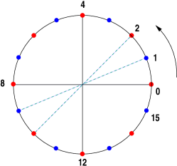
Fig. 1: Using 16 quadrature points for the trapezoidal rule. The set of nodes in the 4-point quadrature is a subset of the nodes of the 8-point quadrature which is itself a subset of the the nodes of the 16-point quadrature rule.

To implement this scheme efficiently, it is best to write the approximation of $f_{j}(z)$ as

$$f_{j}(z)\approx\sum_{i=1}^{m}\frac{\omega_{i}f_{j}(\sigma_{i})}{z-\sigma_{i}}.$$ (27)

Then expression (10) becomes:

$$\widehat{T}(z) =-B_{0}+zA_{0}+\sum_{j=1}^{p}\sum_{i=1}^{m}\frac{\omega_{i}f_{j}(\sigma_{i})}{z-\sigma_{i}}A_{j}=-B_{0}+zA_{0}+\sum_{i=1}^{m}\ \omega_{i}\frac{\sum_{j=0}^{p}f_{j}(\sigma_{i})A_{j}}{z-\sigma_{i}}$$

$$\equiv\ -B_{0}+zA_{0}+\sum_{i=1}^{m}\ \omega_{i}\frac{\widehat{B}_{i}}{z-\sigma_{i}},$$ (28)

where we now set:

$$\widehat{B}_{i}=\sum_{j=0}^{p}f_{j}(\sigma_{i})A_{j},\qquad i=1,\ldots,m.$$ (29)

In other words $B_{i}=\omega_{i}\widehat{B}_{i}$. Note here that although the weights $\omega_{i}$ depend on the level $\ell$, the matrices $\widehat{B}_{i}$ are fixed. In fact when $p$ is small - as is commonly the case - it is best not to store the $\widehat{B}_{i}$’s (or the $B_{i}$’s). Indeed, the matrix $\widehat{B}_{i}$ (as well as $B_{i}$) is only invoked for matrix-vector products (“matvec’s”) which can be carried out with $p$ matvecs using the original matrices $A_{i}$ plus a linear combination of $p$ vectors. If $p$ is large, then it may be advantageous to compute and store the $\widehat{B}_{i}$’s.

3 Theoretical considerations

Let us consider problem (17 – 18) under the simplified assumption that $A_{0}=I$. This is equivalent to having an $A_{0}$ that is invertible, since in this case we can multiply equation (7) by $A_{0}^{-1}$ to reach the desired form in which $A_{0}=I$. Hence, without loss of generality, we assume ${\cal M}=I$.

3.1 Characterization of eigenvalues of ${\cal A}$

Now, we would like to examine all the eigenvalues of matrix ${\cal A}$. For this, we consider the characteristic polynomial of matrix ${\cal A}$. We write ${\cal A}-zI$ as follows:

$${\cal A}-zI=\begin{bmatrix}D-zI&F\\ B^{T}&B_{0}-zI\end{bmatrix},$$ (30)

where, referring to (18), we see that $D$ is $(mn)\times(mn)$, and $F$ and $B$ are both $(mn)\times n$. Then, when $D-zI$ is invertible, i.e., when $z$ is different from all the $\sigma_{i}$’s, the block LU factorization of ${\cal A}-zI$ is given as:

$${\cal A}-zI=\begin{bmatrix}I&0\\ B^{T}(D-zI)^{-1}&I\end{bmatrix}\begin{bmatrix}D-zI&F\\ 0&S(z)\end{bmatrix},$$ (31)

where $S(z)$ is the (spectral) Schur complement:

$$S(z)\equiv B_{0}-zI-B^{T}(D-zI)^{-1}F=B_{0}-zI+\sum_{i=1}^{m}\frac{B_{i}}{\sigma_{i}-z}.$$ (32)

Hence, when $z$ is not a pole, then $\det({\cal A}-zI)=\det(S(z))\det(D-zI).$ Moreover, by comparing equations (10) and (32), we observe that $S(z)=-\widetilde{T}(z)$.

Assume now that $z$ is a pole, e.g., without loss of generality let $z=\sigma_{1}$. In this case, we can use a continuity argument. Indeed, $\det({\cal A}-zI)$ is a continuous function and therefore we can define $\det({\cal A}-zI)$ as the limit:

$$\det({\cal A}-\sigma_{1}I) =\lim_{z\rightarrow\sigma_{1}}\det\left[B_{0}-zI+\sum_{i=1}^{m}\frac{B_{i}}{\sigma_{i}-z}\right]\prod_{i=1}^{m}(\sigma_{i}-z)^{n}$$

$$=\lim_{z\rightarrow\sigma_{1}}\det\left[(\sigma_{1}-z)(B_{0}-zI)+\sum_{i=1}^{m}\frac{\sigma_{1}-z}{\sigma_{i}-z}B_{i}\right]\prod_{i=2}^{m}(\sigma_{i}-z)^{n}$$

$$=\det(B_{1})\prod_{i=2}^{m}(\sigma_{i}-\sigma_{1})^{n}.$$

Note that a second approach to prove the above relation is to observe that when $z=\sigma_{1}$, then the top left $n\times n$ block of ${\cal A}-zI$ is a zero block and this can be exploited to expand the determinant. This result can be generalized to any other $\sigma_{i}$, and therefore we can state the following lemma.

Lemma 1.

The following equality holds :

$$\det({\cal A}-zI)=\left\{\begin{array}[]{lcl}\det(S(z))\prod_{j=1}^{m}(\sigma_{j}-z)^{n}&if&z\neq\sigma_{i}\ \ i=1,\ldots m,\\ \det(B_{i})\prod_{j\neq i}^{m}(\sigma_{j}-\sigma_{i})^{n}&if&z=\sigma_{i}.\end{array}\right.$$ (33)

We denote by $e_{i}$ the $i$-th canonical basis vector of the vector space $\mathbb{C}^{m+1}$ and by $\otimes$ the Kronecker product (operator kron in Matlab). The following corollary is an immediate consequence of Lemma 1.

Corollary 2.

If all the matrices $B_{i},i=0,\ldots,m$ are nonsingular, then the eigenvalues of (12) are the same as the eigenvalues of matrix ${\cal A}$. If a matrix $B_{i}$ is singular and $u$ is an associated null vector, then $\sigma_{i}$ is an eigenvalue of ${\cal A}$ and $e_{i}\otimes u$ is an associated eigenvector.

Hence, we can ignore any eigenvalue that is equal to one of the $\sigma_{i}$’s when it occurs. The next results will show that as long as the rational approximations of the functions $f_{j}:\Omega\rightarrow\mathbb{C}$ are accurate enough, the eigenvalues of $\widetilde{T}(z)$ will be good approximations to all eigenvalues of $T(z)$ located inside the region $\Omega$.

3.2 Accuracy of computed eigenvalues

Let $\Omega_{1}$ be a region strictly included in the (larger) disk $\Omega$ such that $\|f_{j}(z)-r_{j}(z)\|_{\Omega_{1}}<\varepsilon$, where the $\Omega_{1}$-norm is, e.g., the infinity norm in $\Omega_{1}$ and $r_{j}(z)$ is the rational approximation of function $f_{j}(z)$. In other words, each function $f_{j}(z)$ in (6) is approximated by a rational function $r_{j}(z)$ and this approximation is assumed to be accurate within an error of $\varepsilon$ in the region $\Omega_{1}$. Our goal now is to show that each of the eigenvalues inside $\Omega_{1}$ is a ‘good’ approximation to an eigenvalue of the original problem (1). This can be done by exploiting the corresponding approximate eigenvectors and by considering the residual associated with the approximate eigenpair. The following simple proposition shows a result along these lines.

Proposition 3.

Let us assume that $\|f_{j}(z)-r_{j}(z)\|_{\Omega_{1}}\leq\varepsilon$ for $j=1,\cdots,p$ and let $(\widetilde{\lambda},\widetilde{u})$ be an exact eigenpair of the surrogate problem (12) with $\widetilde{\lambda}$ located inside $\Omega_{1}$ and $\|\widetilde{u}\|=1$ for a certain vector norm $\|\cdot\|$.   Let $\mu=\sum\limits_{j=1}^{p}\|A_{j}\|$. Then,

$$\|T(\widetilde{\lambda})\widetilde{u}\|\leq\mu\varepsilon.$$

Proof.

The approximate problem (12) is obtained by replacing $T(z)$ in (7) by:

$$\widetilde{T}(z)=-B_{0}+zA_{0}+r_{1}(z)A_{1}+\ldots+r_{p}(z)A_{p}.$$ (34)

Since $(\widetilde{\lambda},\widetilde{u})$ is an eigenpair of problem (12), $\widetilde{T}({\widetilde{\lambda}})\widetilde{u}=0$, which implies:

$$[-B_{0}+{\widetilde{\lambda}}A_{0}+r_{1}({\widetilde{\lambda}})A_{1}+\ldots+r_{p}({\widetilde{\lambda}})A_{p}]\tilde{u}=0.$$

Setting $f_{j}({\widetilde{\lambda}})-r_{j}({\widetilde{\lambda}})=\eta_{j}({\widetilde{\lambda}})$ and substituting this into above equation gives:

$$[-B_{0}+{\widetilde{\lambda}}A_{0} +\sum_{j=1}^{p}(f_{j}({\widetilde{\lambda}})-\eta_{j}({\widetilde{\lambda}}))A_{j}]{\widetilde{u}}=0,$$

$$[-B_{0}+{\widetilde{\lambda}}A_{0} +\sum_{j=1}^{p}f_{j}({\widetilde{\lambda}})A_{j}]{\widetilde{u}}=\left[\sum_{j=1}^{p}\eta_{j}({\widetilde{\lambda}}))A_{j}\right]{\widetilde{u}},$$

and thus $T({\widetilde{\lambda}}){\widetilde{u}}=\left[\sum_{j=1}^{p}\eta_{j}({\widetilde{\lambda}})A_{j}\right]{\widetilde{u}}.$ Taking norms on both sides and recalling that $\|f_{j}(z)-r_{j}(z)\|_{\Omega_{1}}\leq\varepsilon$ yields $\|T({\widetilde{\lambda}}){\widetilde{u}}\|=\|\sum_{j=1}^{p}\eta_{j}({\widetilde{\lambda}})A_{j}{\widetilde{u}}\|\ \leq\mu\varepsilon,$ which is the desired result. ∎

Proposition 3 implies that any eigenpair of problem (12) is an approximate eigenpair of the original problem provided that each function $f_{j}(z)$ is well approximated by a rational function $r_{j}(z)$ in $\Omega_{1}$ and that the eigenvalue ${\widetilde{\lambda}}$ is inside $\Omega_{1}$. By a backward argument the opposite is also true.

Proposition 4.

Let us assume that $\|f_{j}(z)-r_{j}(z)\|_{\Omega_{1}}\leq\epsilon$ for $j=1,\cdots,p$ and let $(\lambda,u)$ be an exact eigenpair for $T(z)$ with $\lambda$ located inside $\Omega_{1}$ and $\|u\|=1$. Then, $(\lambda,u)$ is an approximate eigenpair of the problem (12), i.e.,

$$\|\widetilde{T}(\lambda)u\|\leq\mu\varepsilon,$$

where $\mu$ is defined as in Proposition 3.

Proof.

The proof is essentially identical to that of Proposition 3. ∎

These two results show that for $\varepsilon$ small enough, we should be able to find approximations to all eigenvalues of the exact problem located in $\Omega_{1}$ (and only these) by solving (12), except for cases of highly ill-conditioned eigenvalues.

3.3 Conditioning of a simple eigenvalue

For the reason stated above, it is of particular importance to examine the condition number of an eigenvalue of the extended problem (17 – 18). There is no loss of generality in assuming that $A_{0}=I$. Let us consider a simple eigenvalue $\lambda$ of the matrix ${\cal A}$. Its right eigenvector is a vector $w$ of the form shown in (16) with $v_{i}=u/(\sigma_{i}-\lambda)$ defined in (13). As seen earlier – equation (12) – the vector $u$ is an eigenvector of $S(\lambda)$, i.e., we have $S(\lambda)u=0.$

The left eigenvector is a vector $s$ that satisfies ${\cal A}^{H}s=\overline{\lambda}s$. Similarly to $w$, it consists of block components $h_{1},\ldots,h_{m},$ and $y$. The equation $({\cal A}^{H}-\overline{\lambda}I)s=0$ yields the relations:

$$(\overline{\sigma}_{i}-\overline{\lambda})h_{i}+B_{i}^{H}y=0\quad\Rightarrow\quad h_{i}=\frac{1}{\overline{\lambda}-\overline{\sigma}_{i}}B_{i}^{H}y,\quad i=1,\ldots,m$$

and

$$-\sum_{i=1}^{m}h_{i}+(B_{0}^{H}-\overline{\lambda}I)y=0\quad\Rightarrow\quad S(\lambda)^{H}y=0.$$

Thus, the right and the left eigenvectors of ${\cal A}$ are defined in terms of the right and the left eigenvectors $u$ and $y$ of $S(\lambda)$.

As is well-known, the condition number of a simple eigenvalue $\lambda$ is the inverse of the cosine of the acute angle between the left and the right eigenvectors. Before considering the inner product $(w,s)$, we point out that the derivative of $S(z)$ is:

$$S^{\prime}(z)=-I+\sum_{i=1}^{m}\frac{B_{i}}{(z-\sigma_{i})^{2}}.$$ (35)

Consider now the inner product $s^{H}w$:

$$s^{H}w=y^{H}u+\sum_{i=1}^{m}h_{i}^{H}v_{i}=y^{H}u-\sum_{i=1}^{m}\frac{y^{H}B_{i}u}{(\lambda-\sigma_{i})^{2}}=-y^{H}S^{\prime}(\lambda)u.$$

Finally, we need to calculate the norms of $s$ and $w$. For $w$ we have:

$$\|w\|_{2}^{2}=\|u\|^{2}+\sum_{i=1}^{m}\frac{\|u\|_{2}^{2}}{|\lambda-\sigma_{i}|^{2}}=\|u\|^{2}\left[1+\frac{1}{|\lambda-\sigma_{i}|^{2}}\right],$$

while for $s$:

$$\|s\|_{2}^{2}=\|y\|^{2}+\sum_{i=1}^{m}\frac{\|B_{i}y\|_{2}^{2}}{|\lambda-\sigma_{i}|^{2}}=\|y\|^{2}\left[1+\sum_{i=1}^{m}\frac{\|B_{i}y\|_{2}^{2}}{\|y\|_{2}^{2}|\lambda-\sigma_{i}|^{2}}\right].$$

Assuming that the vectors $u$ and $y$ are of norm one leads to the following proposition which establishes an expression for the desired condition number.

Proposition 5.

Let $\lambda$ be a simple eigenvalue of (18), and $u,y$ the corresponding unit norm right and left eigenvectors (respectively) of $S(\lambda)$. Then the condition number of $\lambda$ as an eigenvalue of (17 – 18) is given by

$$\kappa(\lambda)=\frac{\alpha_{u}\alpha_{y}}{|(S^{\prime}(\lambda)u,y)|},$$ (36)

where

$$\alpha_{u}=\sqrt{1+\sum_{i=1}^{m}\frac{1}{|\lambda-\sigma_{i}|^{2}}}\qquad\text{ and }\quad\quad\alpha_{y}=\sqrt{1+\sum_{i=1}^{m}\frac{\|B_{i}y\|_{2}}{|\lambda-\sigma_{i}|^{2}}}.$$ (37)

The coefficients $\alpha_{u},\alpha_{y}$ will remain bounded as long as $\lambda$ is far away from any of the poles. Note in particular that the terms $\|B_{i}y\|_{2}$ can be bounded by the constant $\beta=\max_{i}\|B_{i}\|_{2}$. On the other hand nothing will prevent the denominator in (36) from being close to zero. The condition number can be easily gauged to determine if this is the case. Note that $y^{H}S^{\prime}(\lambda)u$ is inexpensive to compute once the eigenvectors $u$ and $y$ are available.

3.4 The halo of extraneous eigenvalues

In all our experiments we observed that the eigenvalues of the problem (17 – 18) that are not eigenvalues of the original nonlinear problem (7) tend to congregate into a ‘halo’ around the contour $\Gamma$ used for the Cauchy integration.

It is possible to explain this phenomenon. First note that the basis of the method under consideration is to approximate the original nonlinear matrix function $T(z)$ in (7) by the rational function:

$$\widetilde{T}(z)=-B_{0}+zA_{0}+r_{1}(z)A_{1}+\ldots+r_{p}(z)A_{p},$$ (38)

where each $r_{j}(z)$ is a rational approximation of $f_{j}(z)$.

Consider the situation when $z$ is outside the domain used to obtain the Cauchy integral, far from the contour. Assuming that the number of quadrature points $m$ is large enough, then each $r_{j}(z)$ will be close to zero. Hence, any eigenvalue of $\widetilde{T}(z)$ that is outside the contour and not too close to it should be just an eigenvalue of the generalized problem $(B_{0}-\lambda A_{0})u=0$. In other words, it should be close to an eigenvalue of the linear part of $T(z)$.

Let us now consider the opposite case of an eigenvalue of $\widetilde{T}(z)$ that is inside the contour but also not too close to it. Our earlier results show that in this case we should only find eigenvalues of the original problem (7) and no other eigenvalues.

For an eigenvalue to be extraneous, i.e., in the spectrum of (17 – 18) but not of (7), it must therefore either be (close to) an eigenvalue of the linear part of $T(z)$, or located (close to) the contour.

Although this argument is based on a simple model, it provides a picture that is remarkably close to what is observed in practice. Next we present an illustration using a small quadratic eigenvalue problem. Quadratic eigenvalue problems can be handled more efficiently by standard linearization than by the method presented in this paper. However, they can be useful for the purpose of validation because their eigenvalues are readily available. Consider the problem

$$(-B_{0}+\lambda A_{0}+\lambda^{2}A_{2})u=0,$$ (39)

where the matrices $B_{0},A_{0},A_{2}$ are generated by the following three Matlab lines of code with $n=4$:

  B0 = -2*eye(n)+diag(ones(n-1,1),1)+diag(ones(n-1,1),-1) ;
  A0 = eye(n);
  A2 = 0.5*(n*eye(n)-eye(n,1)*ones(1,n)-ones(n,1)*eye(1,n));

The eigenvalues are all located inside a rectangle with bottom-left and top-right corners $(-1,-1.5i),(0,1.5i)$ which we use as the integration contour.

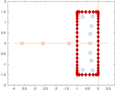
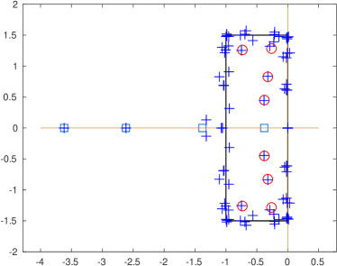
Fig. 2: Left: The $8$ eigenvalues of the original problem (39) (circle); the $4$ eigenvalues of the linear part (square); contour and quadrature points along it. Right: Eigenvalues computed with $m=20$ quadrature points (plus) along with contour, original eigenvalues (circle), and eigenvalues of linear part (square).

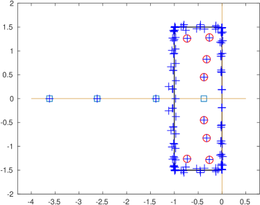
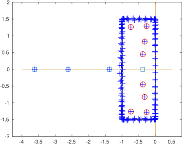
Fig. 3: Same information as in the right part of Figure 2 using a total of $m=32$ quadrature points (left) and $m=60$ quadrature points (right).

Gauss-Legendre quadrature formulas are invoked on each side of the rectangle with a number of points selected to be proportional to the side length. The left side of Figure 2 shows the $8$ eigenvalues of the original problem (7) as well as the $4$ eigenvalues of the pencil $(B_{0},A_{0})$. Three of these eigenvalues are located outside the contour and one inside. The right part of Figure 2 and the two plots in Figure 3 show the eigenvalues of problem (17 – 18) when the number of contour points is $m=20,32,60$, respectively. When $m=20$ the approximations are still rough. However, the pattern mentioned above begins to unravel: the eigenvalues of (39) located inside the contour are more or less approximated, and those eigenvalues of $(B_{0},A_{0})$ that are outside are starting to be neared by pluses. Observe that the eigenvalue of $(B_{0},A_{0})$ that is near $-1.5$ is approximated by two eigenvalues of ${\cal A}$. In contrast, the one near $-0.5$ (inside the contour) is not approximated as predicted by the theory. As $m$ increases this picture is confirmed: (1) all the eigenvalues of (39) inside the contour are well approximated, (2) all the eigenvalues of $(B_{0},A_{0})$ outside the contour are well approximated by eigenvalues of ${\cal A}$, and (3) the eigenvalue of $(B_{0},A_{0})$ inside the contour is essentially ‘ignored’. In addition, the halo of eigenvalues around the contour becomes quite close to the contour itself. This small example provides a good illustration of the general behavior that we observe in our experiments.

4 Numerical Experiments

All the numerical experiments presented in this section were performed with Matlab R2018a. We will illustrate the behavior of Algorithm 2 on several nonlinear eigenvalue problems discussed in [13, 54, 35]. All the examples considered come in the form given in (7). For most of the examples, the contour $\Gamma$ is either circular or rectangular and we seek the eigenvalues closest to the center of $\Gamma$. For Algorithm 2, the shift $\sigma$ is selected to be the center of the region enclosed by the contour $\Gamma$.

In the case of a circular contour, the $m$ quadrature nodes and weights used to perform the numerical integration to approximate the functions $f_{j}$ inside the contour $\Gamma$ were generated using the Gauss-Legendre quadrature rule. To choose a suitable $m$, we take two circles $\Omega_{1}$ and $\Omega$ with the same center and $\Omega_{1}\subset\Omega$. Then, $m$ is increased until the accuracy of the resulting rational approximation is high enough inside $\Omega_{1}$. Note that we need to avoid a region near the outer circle not only because of the poles, but also because the approximations of the $f_{j}$’s will tend to be poor in this region. To illustrate the effectiveness of the proposed approaches, we compare the obtained eigenvalues with the ones obtained by Beyn’s method [13] or/and via a corresponding linearization. We also compare our algorithm with some well-established nonlinear eigensolvers utilizing rational approximation, i.e., the set-valued AAA algorithm [50] and the NLEIGS [28].

Example 1

Consider the following example discussed in [49, Sec. 2.4.2] and [35, Example 13],

$$T(z)=-B_{0}+zI+e^{-z\tau}A_{1},$$ (40)

with $B_{0}=\begin{pmatrix}-5&1\\ 2&-6\end{pmatrix}$, $A_{1}=-\begin{pmatrix}-2&1\\ 4&-1\end{pmatrix}$ and $\tau=1$. The nonlinear eigenvalue problem (40) is the characteristic equation of a delay system $x^{\prime}(t)=-B_{0}x(t)+A_{1}x(t-\tau)$. For the purpose of a comparison with the results from [13, Example 5.5], we calculate all eigenvalues enclosed by a circle centered at $c=-1$ with radius $r=6$. Referring to Proposition 3, we first check which values of $m$ will provide a good rational approximation $r_{m}(z)$ of $f(z)=e^{-z}$. The right part of Figure 4 shows the errors $e_{m}=\|f(z)-r_{m}(z)\|_{\infty}$ (evaluated on a finely discretized version of $\Omega_{1}$) versus the number of quadrature nodes $m$. Notice that the accuracy of the rational approximation of $f(z)$ inside the considered contour is good enough for $m=50$. We can therefore solve the eigenvalue problem (17), associated with the approximate problem (12), with $m=50$ Gauss-Legendre quadrature nodes. The left part of Figure 4 compares the eigenvalues computed by applying the shift-and-invert Arnoldi method to the large system (17 – 18) with $m=50$ quadrature nodes and those computed by Beyn’s method using the same contour. Note that since the number of eigenvalues in the considered contour is larger than the size of problem (40), we use Beyn’s second algorithm with three moments to compute the five eigenvalues with the backward error smaller than $\delta=10^{-10}$. With these parameters, the number of quadrature nodes for Beyn’s method necessary to get the five eigenvalues inside the circle is $80$.

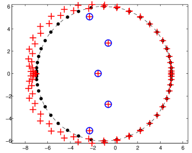
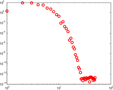
Fig. 4: Left: Eigenvalues of (40) inside a circle of radius $r=6$ centered at $c=-1$ obtained by solving the eigenvalue problem (17) (plus) using $m=50$ quadrature nodes (point) and by Beyn’s method (circle) using $150$ quadrature nodes. Right: The errors $e_{m}$ of the rational approximation of $e^{-z}$ versus the number of quadrature nodes $m$.

In order to check the conclusions of Proposition 3, we compute again all the eigenvalues of the generalized eigenvalue problem (17) associated with the approximate problem (12) inside a circle $\Omega$ centered at $c=-1$ with radius $r=6$, using $m=100$ quadrature nodes. These eigenvalues are shown on the left side of Figure 5. Let $\Omega_{1}$ be a disk with the same center as $\Omega$ and with radius $r_{1}=r/2$. Let $\lambda_{1}$ be the closest eigenvalue to $c$ located in $\Omega_{1}$ and $u_{1}$ be the corresponding eigenvector. Recall that $u_{1}$ is taken from the last $n$ entries of the eigenvector corresponding to the eigenvalue $\lambda_{1}$ of (17). Let $\mu$ be the constant from Proposition 3 and $r_{m}(z)$ the rational approximation of the function $f(z)=e^{-z}$. The right side of Figure 5 compares the residuals $\|T(\lambda_{1})u_{1}\|_{\infty}$ with the errors $e_{m}=\mu\|f(z)-r_{m}(z)\|_{\infty}$ when the number of quadrature nodes $m$ varies.

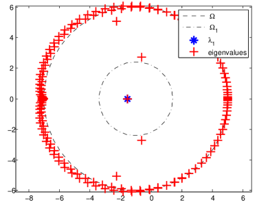
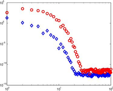
Fig. 5: Left: All eigenvalues of (40) (plus) computed via (17). Right: Residuals $\|T(\lambda_{1})u_{1}\|_{\infty}$ (diamond) and errors $e_{m}$ (circle) versus the number of quadrature nodes $m$.

Example 2

In this experiment, we consider the same nonlinear eigenvalue problem as in Example 1 with a different search contour. The location of the eigenvalues in Example 1 suggests that it should be more effective to consider a rectangular contour instead of a disk. An advantage of rectangular regions is that they are easier to subdivide into smaller rectangular regions than disks. For example, we can split a rectangle in the complex plane into different sub-rectangles and then apply Algorithm 2 in each sub-rectangle. A side benefit of this approach is the added parallelism since each sub-rectangle can be processed independently. Finally, this divide-and-conquer approach also allows to take advantage of the trade-off between using smaller regions which require fewer poles versus larger regions which will yield more eigenvalues at once at the cost of using more poles. If $c_{1},c_{2},c_{3},c_{4}$ are the four corners of the rectangle, listed counter clock-wise with $c_{1}$ being the top-left corner, the integration starts at $c_{1}$, and is performed counterclockwise using Gauss-Legendre quadrature on each side. To solve the nonlinear eigenvalue problem (40), we consider the rectangle defined by the two opposite corners at $c_{2}=-3-6\imath$ and $c_{4}=1+6\imath$, and we solve the eigenvalue problem (17) directly, using $m=40$ quadrature points. The left part of Figure 6 shows that all eigenvalues are well approximated inside the rectangle. To illustrate the behavior of the rational approximation method for the nonlinear eigenvalue problem near the nodes, we consider a smaller rectangle defined by $c_{2}=-2.5-6\imath$ and $c_{4}=-0.2+6\imath$. As we can clearly see on the right side of Figure 6, eigenvalues near the quadrature nodes are not well approximated. This is a consequence of the poor rational approximation of the function $f(z)=e^{-z}$ near the quadrature nodes. Good eigenvalue approximations can be computed by increasing the number of quadrature nodes on each side. This is illustrated in Figure 7 in which $m=50$ quadrature nodes are considered.

Even though for some problems rectangular (non-circular) contours may seem to be better suited, they do not yield an exponential increase in accuracy as the number of quadrature points increases as is the case for the trapezoidal rule on circular contours [66, Theorem 2.1]. They are also more tedious to implement.

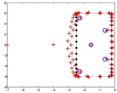
Fig. 6: Left: Eigenvalues of (40) obtained by solving the eigenvalue problem (17) (plus) inside a rectangle defined by $c_{2}=-3-6\imath$ and $c_{4}=1+6\imath$ with $m=40$ quadrature nodes (point) obtained by Beyn’s method (circle) Right: Eigenvalues of (40) obtained by solving the eigenvalue problem (17) (plus) inside a rectangle defined by $c_{2}=-2.5-6\imath$ and $c_{4}=-0.2+6\imath$ with $m=40$ quadrature nodes (point) obtained by Beyn’s method (circle).

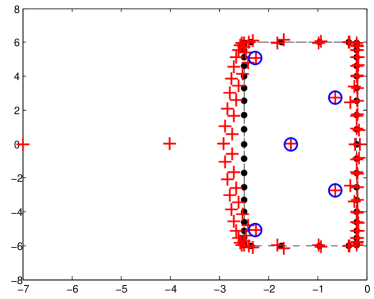
Fig. 7: Eigenvalues of (40) obtained by solving the eigenvalue problem (17) (plus) inside a rectangle defined by $c_{2}=-2.5-6\imath$ and $c_{4}=-0.2+6\imath$ with $m=50$ quadrature nodes (point) and by Beyn’s method (circle).

Example 3: Hadeler problem

As an example of a general nonlinear eigenvalue problem, we consider the Hadeler problem [30, 54, 11]:

$$T(z)=(e^{z}-1)B_{1}+z^{2}B_{2}-B_{0},$$ (41)

with the coefficient matrices

$$B_{0}=b_{0}I,\ \ \ B_{1}=(b^{(1)}_{jk}),\ \ B_{2}=(b^{(2)}_{jk}),$$ (42)

$$b^{(1)}_{jk}=(n+1-\max(j,k))jk,\ \ \ b^{(2)}_{jk}=n\delta_{jk}+1/(j+k),$$ (43)

of dimension $n$ and a parameter $b_{0}=100$ (following reference [54]). For our experiments we choose $n=200$. Note that the theoretical considerations in Section 3 assumed the matrix $A_{0}$ to be invertible, this example shows that our algorithm can be used for solving more general problems.

We refer the reader to the above articles for details on this problem. The eigenvalues of (41) are real with $n$ of them being negative and $n$ positive. The eigenvalues become better spaced as we move away from the origin and the smallest one is close to $-48$. We compute the eigenvalues inside a circle centered at $c=-30$ with radius $r=11.5$. We first determine the number of quadrature nodes $m$ necessary to get a good rational approximations of functions $f_{1}(z)=e^{z}-1$ and $f_{2}(z)=z^{2}$ inside the considered circular contour $\Gamma$. The right part of Figure 8 shows the approximation errors for the rational approximations of $f_{1}(z)$ and $f_{2}(z)$ versus $m$. Based on Figure 8 and referring to proposition 3, a degree of $m=32$ is sufficient to approximate $T(z)$ up to the accuracy of $\mathrm{tol}=10^{-12}$. Using $m=32$ Gauss-Legendre quadrature nodes, $12$ eigenvalues of (41) were computed using shift-and-invert Arnoldi method applied to the large system (17–18). These results are compared with the approximations obtained by Beyn’s first algorithm [13], see left side of Figure 8. For Beyn’s method, $50$ quadrature points are required to reach a backward error of the $12$ eigenvalues smaller than $\delta=10^{-10}$.

We repeat the same experiment using the reduced subspace iteration given by Algorithm 2. We first start with $\nu=40$ random vectors, where $\nu$ is the dimension of the subspace in Algorithm 2 and then apply $q=10$ steps of inverse iteration method, i.e., Algorithm 1, on each of these vectors separately to obtain a block of $\nu$ vectors each one of size $n$. Note that these vectors are the resulting bottom parts of the final iterates of Algorithm 1. These $\nu$ bottom parts are orthogonalized to obtain an orthonormal basis $U$ used to perform the Rayleigh-Ritz projection that leads to a nonlinear eigenvalue problem in $\mathbb{C}^{\nu}$ of the form (26). We then solve this reduced (nonlinear) eigenvalue problem (26) by computing the eigenvalues and eigenvectors of the corresponding expanded problem (17 – 18). Note that this projected problem is now of size $(m+1)\nu\ll(m+1)n$. Before each restart of Algorithm 2, we select $\nu$ approximate eigenpairs whose eigenvalues are inside the contour. The initial vectors $w$ selected in line 3 of the Algorithm 2 are of the form $w=[v;\ u]$ where the components $v_{i}$ of $v$ satisfy $v_{i}=u/(\sigma_{i}-\lambda)$. Here $(\lambda,u)$ is one of the $\nu$ approximate eigenpairs computed from the previous outer iteration. At the very first outer iteration $v$ and $u$ are random vectors. The resulting bottom parts of the final iterates are used to form the block $U$, see line 5 of Algorithm 2. The columns of $U$ are orthonormalized before applying the Rayleigh-Ritz procedure in lines 6–7. At each level $\ell$ we use $2^{\ell-1}$ quadrature points. This multilevel approach allows us to obtain several (coarse) approximations, one for each level $\ell$, using the same set of $m=32$ (fine) quadrature points. Algorithm 2 computed the $12$ eigenvalues of interest requiring $L=6$ outer iterations. These results are compared with the approximations obtained by the AAA algorithm [50] and the NLEIGS algorithm [28], see Figure 9. For the AAA and NLEIGS algorithms, the boundary circle is discretized by $100$ equispaced points and an error tolerance of $10^{-12}$ is set for the rational interpolant. Note that $7$ and $38$ interpolation nodes are needed to approximate $T(z)$ up to the accuracy of $\mathrm{tol}=10^{-12}$ inside the circle, using the AAA and the NLEIGS algorithm, respectively. Finally the right side of Figure 9 illustrates the nonlinear residual norm $\|T(\lambda)u\|_{\infty}$ for all $12$ eigenpairs $(\lambda,u)$ computed by Algorithm 2, and those computed by the AAA and the NLEIGS algorithm.

Another way to extract those $12$ eigenvalues of interest is to resort to the rational approximation using the Cauchy integral formula inside an elliptic contour. We consider an ellipse centered at $c=-30$ with semi-major axis $r_{x}=10$ and semi-minor axis $r_{y}=1$ on the $x$-axis and $y$-axis, respectively. We can solve the expanded problem (17 – 18) with $m=8$ and $\sigma=c$ and perform as many steps as needed to extract all $12$ real eigenvalues inside the elliptic contour. In Figure 10, we present the eigenvalues obtained solving the expanded problem (17 – 18) using Algorithm  2 and Beyn’s integral method with the same elliptic contour. For Beyn’s method $20$ trapezoidal quadrature nodes are necessary to compute all $12$ eigenvalues of interest with the backward error smaller than $\delta=10^{-10}$.

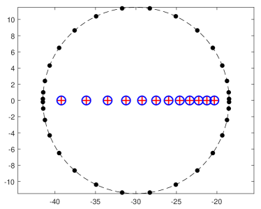
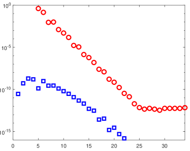
Fig. 8: Left: Eigenvalues of (41) inside a circle of radius $r=11.5$ and center $c=-30$ obtained by computing the eigenvalues of the expanded problem (17 – 18) (plus) and by Beyn’s method (circle). Right: The errors $e_{m}$ of the rational approximation of $e^{-z}$ (square) and $z^{2}$ (circle) versus the number of quadrature nodes $m$.

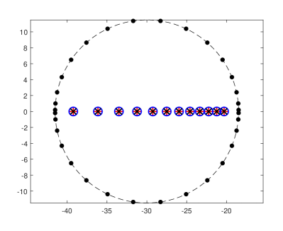
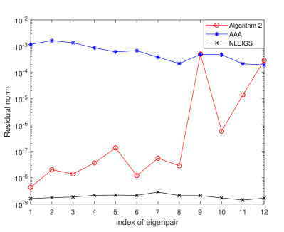
Fig. 9: Left: Eigenvalues of (41) inside a circle of radius $r=11.5$ and center $c=-30$ obtained by Algorithm 2 (plus), the AAA algorithm (circle) and the NLEIGS algorithm (cross). Right: The residual norm $\|T(\lambda)u\|_{\infty}$ of the computed eigenpairs.

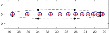
Fig. 10: Eigenvalues of (41) inside an ellipse centered at $c=-30$ and with semi-major axis $r_{x}=10$ and semi-minor axis $r_{y}=1$ obtained by solving the expanded problem (17 – 18) (plus) and by Beyn’s method (circle).

5 Concluding remarks

An appealing feature of the general approach proposed in this paper for solving nonlinear eigenvalue problems is its simplicity. A general nonlinear problem is approximated by a rational eigenvalue problem which is then linearized. The resulting linear problem provides the basis for developing a number of methods and one of them, among possibly many others, is discussed in this paper. The theory allows to exactly predict which eigenvalues of the original problem are well approximated and to ensure that no eigenvalues in the region will be missed. Another attribute of the proposed method is its flexibility. It is possible to compute all eigenvalues in a union of small regions each requiring a small number of poles, or to use one single large region to compute many eigenvalues but now with a large number of poles. The question as to how to optimally exploit these trade-offs remains to be further investigated. Finally, the method has a good potential for solving realistic large sparse nonlinear eigenvalue problems such as those mentioned in the introduction. For more details, we refer the reader to [21]. In this regard, we note that only one factorization is required namely that of $S(\sigma)$ where $\sigma$ is the shift in the shift-and-invert procedure. In many applications the patterns of the matrices $A_{j}$ are not too different from one another and so $S(\sigma)$, which is itself a combination of the $A_{j}$s, will remain sparse.

Appendix A Additional Numerical Experiments

Example 4

We consider the following nonlinear eigenvalue problem, see [59, 35],

$$T(z)=B_{0}+zA_{0}+\frac{1}{1-z}e_{n}e_{n}^{T},$$ (44)

with

$$B_{0}=n\begin{pmatrix}2&-1&&&\\ -1&\ddots&\ddots&\\ &\ddots&2&-1\\ &&-1&1\end{pmatrix},\quad A_{0}=-\frac{1}{6n}\begin{pmatrix}4&1&&&\\ 1&\ddots&\ddots&\\ &\ddots&4&1\\ &&1&2\end{pmatrix},$$

resulting from the finite element discretization of the nonlinear boundary eigenvalue problem

$$-u^{\prime\prime}(x)=\lambda u(x),0\leq x\leq 1,\quad u(0)=u^{\prime}(1)+\frac{\lambda}{\lambda-1}u(1)=0.$$ (45)

To compare our results with those obtained by Beyn’s method [13, Example 4.11], we consider the case when $n=100$ and compute five eigenvalues enclosed by a circle centered at $c=150$ with radius $r=150$. We first determine the number of quadrature nodes $m$ needed to get a good rational approximation of the function $f(z)=\frac{1}{1-z}$ inside the considered circular contour $\Gamma$. The right part of Figure 11 shows the approximation error for the rational approximation of $f(z)$ versus $m$.

Because $f(z)$ is itself a rational function a high enough accuracy is obtained for a small value of $m$, namely $m=6$. Therefore, we solve the expanded problem (17 – 18) with $m=6$ and $\sigma=c$ to get the approximate eigenvalues inside the circle. The computed eigenvalues are shown on the left of Figure 11. These results are directly compared with the ones obtained by Beyn’s first algorithm with the backward error of the $5$ eigenvalues being smaller than $\delta=10^{-4}$. To obtain this level of accuracy, $50$ quadrature nodes are needed to determine the $5$ eigenvalues inside the circle.

Note that the function $f(z)$ is already given in a rational form and so we can solve (44) by considering the same linearization as the one invoked in Section 2:

$$\begin{bmatrix}I&-I\\ e_{n}e_{n}^{T}&B_{0}\end{bmatrix}\begin{bmatrix}\frac{u}{1-z}\\ u\end{bmatrix}=z\begin{bmatrix}I&0\\ 0&-A_{0}\end{bmatrix}\begin{bmatrix}\frac{u}{1-z}\\ u\end{bmatrix}.$$ (46)

Figure 12 compares the eigenvalues obtained by solving (46) and the ones obtained by computing the eigenvalues and of the expanded problem (17 – 18).

Alternatively, we can solve problem (44) directly using Algorithm 2 without restarts, i.e., with only one outer loop ($\ell=1$ only). Let $w_{i}=[v_{i};\ u_{i}]$, $i=1,...,\nu$ be a set of $\nu$ random vectors of size $N=(m+1)n$, where $v_{i}\in\mathbb{R}^{mn}$ and $u_{i}\in\mathbb{R}^{n}$. For this experiment, we choose $\nu=7$ and we apply $q=5$ steps of Algorithm 1 on each $w_{i}$. We orthogonalize the resulted vectors $U=[u_{1},u_{2},\ldots,u_{\nu}]$ to obtain a good subspace to perform the projection method introduced in Algorithm 2.

We set $m=6$ and invoke one outer iteration of Algorithm 2 to compute the eigenvalues enclosed by the same circular contour. As can be seen on the left of Figure 12, the eigenvalues obtained are in good agreement with those obtained by computing the eigenvalues of the expanded problem (17 – 18) and by Beyn’s method.

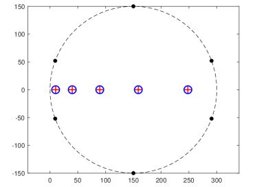
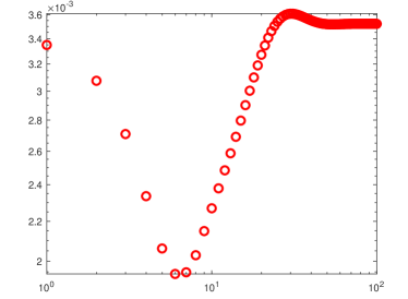
Fig. 11: Left: Eigenvalues of (44) inside a circle of radius $r=150$ centered at $c=150$ obtained by computing the eigenvalues of the expanded problem (17 – 18) (plus) and by Beyn’s method (circle). Right: The errors $e_{m}$ of the rational approximation of $f(z)=\frac{1}{1-z}$ versus the number of quadrature nodes $m$.

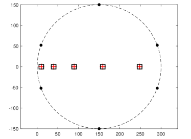
Fig. 12: Left: Eigenvalues of (44) inside a circle of radius $r=150$ centered at $c=150$ obtained by Algorithm 2 (plus) and by Beyn’s method (circle). Right: Eigenvalues of (44) inside a circle of radius $r=150$ centered at $c=150$ obtained by computing the eigenvalues of the expanded problem (17 – 18) (plus) and by linearization (46) (square).

Example 5: Butterfly Problem

To illustrate the behavior of rational approximation methods when using a contour centered at an arbitrary point in the complex plane, we present a few results with the butterfly problem (so called because of the distribution of its eigenvalues in the complex plane) available from the NLEVP collection [11]. This is a quartic eigenvalue problem of the form

$$T(\lambda)=A_{0}+\lambda A_{1}+\lambda^{2}A_{2}+\lambda^{3}A_{3}+\lambda^{4}A_{4},$$ (47)

where $A_{0},A_{1},\ldots,A_{4}$ are structured matrices of size $n=64$. The $256$ eigenvalues of this problem are shown on the left side of Figure 13. A detailed description of this example can be found in [48]. We compute the eigenvalues and vectors of the expanded problem (17 – 18) with $m=50$ quadrature nodes to compute the eigenvalues enclosed by a circle centered at $c=1+1\imath$ with radius $r=0.5$. We compare approximations of $13$ computed eigenvalues with those determined by the linearization of problem (47) and by application of Beyn’s method. The right part of Figure 13 summarizes our findings. Alternatively, we can use a rectangular contour as described already in Example 2. Figure 14 shows approximations of $17$ eigenvalues enclosed by the rectangular contour defined by the corners $c_{2}=(0.55,0.48)$ and $c_{4}=(1.2,1.3)$ obtained by solving the expanded problem (17 – 18) with $m=90$ quadrature nodes and direct linearization.

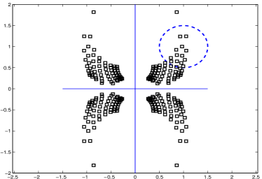
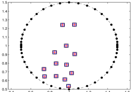
Fig. 13: Left: All $256$ eigenvalues of butterfly example (47) (square) obtained by linearization. Circle contour centered at $c=1+1\imath$ with radius $r=0.5$ (dashed). Right: Eigenvalues of butterfly example (47) inside a circle of radius $r=0.5$ centered at $c=1+1\imath$ obtained by computing the eigenvalues of the expanded problem (17 – 18) (plus) with $m=50$, by linearization (square) and by Beyn’s method (circle).

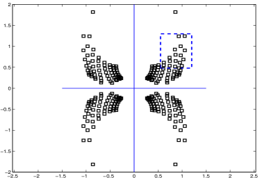
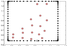
Fig. 14: Left: All $256$ eigenvalues of butterfly example (47) (square) obtained by linearization. Rectangular contour centered at $0.875+0.89\imath$ with corners $(0.55,1.3),(0.55,0.48),(1.2,0.48)$ and $(1.2,1.3)$ (dashed). Right: Eigenvalues of butterfly example (47) inside a rectangular contour obtained by computing the eigenvalues of the expanded problem (17 – 18) (plus) with $m=90$ and by linearization.

References

- [1] A. Amiraslani, R. M. Corless, and P. Lancaster, Linearization of matrix polynomials expressed in polynomial bases, IMA J. Numer. Anal., 29 (2009), pp. 141–157.
- [2] E. N. Antoniou and S. Vologiannidis, A new family of companion forms of polynomial matrices, Electron. J. Linear Algebra, 11 (2004), pp. 78–87.
- [3] T. Apel, V. Mehrmann, and D. Watkins, Numerical solution of large scale structured polynomial or rational eigenvalue problems, in Foundations of computational mathematics: Minneapolis, 2002, vol. 312 of London Math. Soc. Lecture Note Ser., Cambridge Univ. Press, Cambridge, 2004, pp. 137–156.
- [4] J. Asakura, T. Sakurai, H. Tadano, T. Ikegami, and K. Kimura, A numerical method for nonlinear eigenvalue problems using contour integrals, JSIAM Lett., 1 (2009), pp. 52–55.
- [5] M. Van Barel, Designing rational filter functions for solving eigenvalue problems by contour integration, Linear Algebra Appl., 502 (2016), pp. 346–365.
- [6] M. Van Barel and P. Kravanja, Nonlinear eigenvalue problems and contour integrals, J. Comput. Appl. Math., 292 (2016), pp. 526–540.
- [7] R. Van Beeumen, Rational Krylov Methods for Nonlinear Eigenvalue Problems, PhD thesis, Department of Computer Science, KU Leuven, Belgium, 2015.
- [8] R. Van Beeumen, O. Marques, E. G. Ng, C. Yang, Z. Bai, L. Ge, O. Kononenko, Z. Li, C.-K. Ng, and L. Xiao, Computing resonant modes of accelerator cavities by solving nonlinear eigenvalue problems via rational approximation, J. Comput. Phys., 374 (2018), pp. 1031–1043.
- [9] R. Van Beeumen, K. Meerbergen, and W. Michiels, A rational Krylov method based on Hermite interpolation for nonlinear eigenvalue problems, SIAM J. Sci. Comput., 35 (2013), pp. A327–A350.
- [10] , Compact rational Krylov methods for nonlinear eigenvalue problems, SIAM J. Matrix Anal, 36 (2015), pp. 820–838.
- [11] T. Betcke, N. J. Higham, V. Mehrmann, C. Schröder, and F. Tisseur, NLEVP: a collection of nonlinear eigenvalue problems, ACM Trans. Math. Software, 39 (2013), pp. Art. 7, 28.
- [12] T. Betcke and H. Voss, A Jacobi–Davidson-type projection method for nonlinear eigenvalue problems, Future Gener. Comput. Syst., 20 (2004), pp. 363–372.
- [13] W.-J. Beyn, An integral method for solving nonlinear eigenvalue problems, Linear Algebra Appl., 436 (2012), pp. 3839–3863.
- [14] W.-J. Beyn, C. Effenberger, and D. Kressner, Continuation of eigenvalues and invariant pairs for parameterized nonlinear eigenvalue problems, Numer. Math., 119 (2011), pp. 489–516.
- [15] P. Bharadwaj, B. Deutsch, and L. Novotny, Optical antennas, Adv. Opt. Photonics., 1 (2009), pp. 438–483.
- [16] F. M. Dopico and J. González-Pizarro, A compact rational Krylov method for large-scale rational eigenvalue problems, Numer. Linear Algebra Appl., 26 (2018), pp. e2214, 26.
- [17] F. M. Dopico, P. W. Lawrence, J. Pérez, and P. Van Dooren, Block Kronecker linearizations of matrix polynomials and their backward errors, Numer. Math., 140 (2018), pp. 373–426.
- [18] F. M. Dopico, J. Pérez, and P. Van Dooren, Structured backward error analysis of linearized structured polynomial eigenvalue problems, Math. Comp., 88 (2019), pp. 1189–1228.
- [19] C. Effenberger, Robust successive computation of eigenpairs for nonlinear eigenvalue problems, SIAM J. Matrix Anal. Appl., 34 (2013), pp. 1231–1256.
- [20] C. Effenberger, Robust successive computation of eigenpairs for nonlinear eigenvalue problems, SIAM J. Matrix Anal. Appl., 34 (2013), pp. 1231–1256.
- [21] M. El-Guide, A. Międlar, and Y. Saad, A rational approximation method for solving acoustic nonlinear eigenvalue problems, Eng. Anal. Bound. Elem., 111 (2020), pp. 44–54.
- [22] M. Embree, Nonlinear eigenvalue problems: Interpolatory algorithms and transient dynamics. SIAM Conference on Applied Linear Algebra, Hong Kong, May 2018.
- [23] H. Faßbender and P. Saltenberger, Block Kronecker ansatz spaces for matrix polynomials, Linear Algebra Appl., 542 (2018), pp. 118–148.
- [24] M. Fiedler, A note on companion matrices, Linear Algebra Appl., 372 (2003), pp. 325–331.
- [25] B. Gavin, A. Miedlar, and E. Polizzi, FEAST eigensolver for nonlinear eigenvalue problems, J. Comput. Sci., 27 (2018), pp. 107–117.
- [26] I. Gohberg, P. Lancaster, and L. Rodman, Matrix polynomials, vol. 58 of Classics in Applied Mathematics, Society for Industrial and Applied Mathematics (SIAM), Philadelphia, PA, 2009. Reprint of the 1982 original [ MR0662418].
- [27] G. H. Golub and C. F. Van Loan, Matrix computations, Johns Hopkins Studies in the Mathematical Sciences, Johns Hopkins University Press, Baltimore, MD, fourth ed., 2013.
- [28] S. Güttel, R. Van Beeumen, K. Meerbergen, and W. Michiels, NLEIGS: a class of fully rational Krylov methods for nonlinear eigenvalue problems, SIAM J. Sci. Comput., 36 (2014), pp. A2842–A2864.
- [29] S. Güttel and F. Tisseur, The Nonlinear Eigenvalue Problem, Acta Numer., 26 (2017), pp. 1–94.
- [30] K. P. Hadeler, Mehrparametrige und nichtlineare Eigenwertaufgaben, Arch. Ration. Mech. Anal, 27 (1967), pp. 306–328.
- [31] N. J. Higham, D. S. Mackey, N. Mackey, and F. Tisseur, Symmetric linearizations for matrix polynomials, SIAM J. Matrix Anal. Appl., 29 (2006/07), pp. 143–159.
- [32] T.-M. Hwang, W.-W. Lin, W.-C. Wang, and W. Wang, Numerical simulation of three dimensional pyramid quantum dot, J. Comput. Phys., 196 (2004), pp. 208–232.
- [33] E. Jarlebring, W. Michiels, and K. Meerbergen, A linear eigenvalue algorithm for the nonlinear eigenvalue problem, Numer. Math., 122 (2012), pp. 169–195.
- [34] T. Klimpel, Verschließ im Rad-/Schiene Kontakt infolge mittel- und hochfrequenter, dynamischer Beanspruchungen, PhD Thesis, TU Berlin, Institut für Lunft- und Raumfahrt, Germany, 2003.
- [35] D. Kressner, A block Newton method for nonlinear eigenvalue problems, Numer. Math., 114 (2009), pp. 355–372.
- [36] V. N. Kublanovskaya, On an approach to the solution of the generalized latent value problem for -matrices, SIAM J. Numer. Anal., 7 (1970), pp. 532–537.
- [37] P. Lancaster, A generalised Rayleigh quotient iteration for lambda-matrices, Arch. Ration. Mech. Anal., 8 (1961), pp. 309–322.
- [38] , Lambda-matrices and vibrating systems, Dover Publications, Inc., Mineola, NY, 2002. Reprint of the 1966 original [Pergamon Press, New York; MR0210345 (35 #1238)].
- [39] P. Lietaert, K. Meerbergen, and F. Tisseur, Compact two-sided Krylov methods for nonlinear eigenvalue problems, SIAM J. Sci. Comput., 40 (2018), pp. A2801–A2829.
- [40] P. Lietaert, J. Pérez, B. Vandereycken, and K. Meerbergen, Automatic rational approximation and linearization of nonlinear eigenvalue problems, arXiv e-prints, (2018), p. arXiv:1801.08622.
- [41] D. Lu, Y. Su, and Z. Bai, Stability analysis of the two-level orthogonal Arnoldi procedure, SIAM J. Matrix Anal. Appl., 37 (2016), pp. 195–214.
- [42] D. S. Mackey, Structured linearizations for matrix polynomials, PhD thesis, Manchester, UK, 2006.
- [43] , The continuing influence of Fiedler’s work on companion matrices, Linear Algebra Appl., 439 (2013), pp. 810–817.
- [44] D. S. Mackey, N. Mackey, C. Mehl, and V. Mehrmann, Structured polynomial eigenvalue problems: good vibrations from good linearizations, SIAM J. Matrix Anal. Appl., 28 (2006), pp. 1029–1051.
- [45] , Vector spaces of linearizations for matrix polynomials, SIAM J. Matrix Anal. Appl., 28 (2006), pp. 971–1004.
- [46] D. S. Mackey, N. Mackey, and F. Tisseur, Polynomial eigenvalue problems: theory, computation, and structure, in Numerical algebra, matrix theory, differential-algebraic equations and control theory, Springer, Cham, 2015, pp. 319–348.
- [47] V. Mehrmann and H. Voss, Nonlinear eigenvalue problems: a challenge for modern eigenvalue methods, GAMM Mitt. Ges. Angew. Math. Mech., 27 (2004), pp. 121–152 (2005).
- [48] V. Mehrmann and D. Watkins, Polynomial eigenvalue problems with Hamiltonian structure, Electron. Trans. Numer. Anal., 13 (2002), pp. 106–118.
- [49] W. Michiels and S.-I. Niculescu, Stability and stabilization of time-delay systems, vol. 12 of Advances in Design and Control, Society for Industrial and Applied Mathematics (SIAM), Philadelphia, PA, 2007. An eigenvalue-based approach.
- [50] Y. Nakatsukasa, O. Sète, and L. N. Trefethen, The AAA algorithm for rational approximation, SIAM J. Sci. Comput., 40 (2018), pp. A1494–A1522.
- [51] A. Neumaier, Residual inverse iteration for the nonlinear eigenvalue problem, SIAM J. Numer. Anal., 22 (1985), pp. 914–923.
- [52] E. Polizzi, A density matrix-based algorithm for solving eigenvalue problems, Phys. Rev. B, 79 (2009).
- [53] L. Robol, R. Vandebril, and P. Van Dooren, A framework for structured linearizations of matrix polynomials in various bases, SIAM J. Matrix Anal. Appl., 38 (2017), pp. 188–216.
- [54] A. Ruhe, Algorithms for the nonlinear eigenvalue problem, SIAM J. Numer. Anal., 10 (1973), pp. 674–689.
- [55] , Rational Krylov sequence methods for eigenvalue computation, Linear Algebra Appl., 58 (1984), pp. 391–405.
- [56] , Rational Krylov: a practical algorithm for large sparse nonsymmetric matrix pencils, SIAM J. Sci. Comput., 19 (1998), pp. 1535–1551.
- [57] K. Schreiber, Nonlinear Eigenvalue Problems: Newton-type Methods and Nonlinear Rayleigh Functionals, PhD thesis, Technische Universität Berlin, Germany, 2008.
- [58] G. L. Sleijpen, A. G. L. Booten, D. K. Fokkema, and H. A. Van der Vorst, Jacobi-Davidson type methods for generalized eigenproblems and polynomial eigenproblems, BIT, 36 (1996), pp. 595–633. International Linear Algebra Year (Toulouse, 1995).
- [59] S. I. Solov’ëv, Preconditioned iterative methods for a class of nonlinear eigenvalue problems, Linear Algebra Appl., 415 (2006), pp. 210–229.
- [60] Y. Su and Z. Bai, Solving rational eigenvalue problems via linearization, SIAM J. Matrix Anal. Appl., 32 (2011), pp. 201–216.
- [61] Y. Su, J. Zhang, and Z. Bai, A compact Arnoldi algorithm for polynomial eigenvalue problems, Recent Advances in Numerical Methods for Eigenvalue Problems (RANMEP2008), Taiwan, (2008), p. 120.
- [62] F. De Terán and F. M. Dopico, Sharp lower bounds for the dimension of linearizations of matrix polynomials, Electron. J. Linear Algebra, 17 (2008), pp. 518–531.
- [63] F. De Terán, F. M. Dopico, and D. S. Mackey, Fiedler companion linearizations and the recovery of minimal indices, SIAM J. Matrix Anal. Appl., 31 (2009/10), pp. 2181–2204.
- [64] , Spectral equivalence of matrix polynomials and the index sum theorem, Linear Algebra Appl., 459 (2014), pp. 264–333.
- [65] F. Tisseur and K. Meerbergen, The quadratic eigenvalue problem, SIAM Rev., 43 (2001), pp. 235–286.
- [66] L. N. Trefethen and J. A. C. Weideman, The exponentially convergent trapezoidal rule, SIAM Rev., 56 (2014), pp. 385–458.
- [67] H. Unger, Nichtlineare Behandlung von Eigenwertaufgaben, ZAMM Z. Angew. Math. Mech., 30 (1950), pp. 281–282.
- [68] K. J. Vahala, Optical microcavities, Nature, 424 (2003), pp. 839–846.
- [69] H. Voss, Iterative projection methods for computing relevant energy states of a quantum dot, J. Comput. Phys., 217 (2006), pp. 824–833.
- [70] , Nonlinear Eigenvalue Problems - Chapter 60, in Handbook of Linear Algebra, Second Edition, L. Hogben, ed., Discrete Mathematics and its Applications, Chapman & Hall/CRC, Boca Raton, FL, 2013, pp. 1063–1086.
- [71] S. Yokota and T. Sakurai, A projection method for nonlinear eigenvalue problems using contour integrals, JSIAM Lett., 5 (2013), pp. 41–44.