Interplay of the CGC and TMD frameworks to all orders in kinematic twist

Abstract

A framework for an improved TMD (iTMD) factorization scheme at small $x$, involving off-shell perturbative subamplitudes, was recently developed as an interpolation between the TMD $k_{t}\ll Q$ regime and the BFKL $k_{t}\sim Q$ regime. In this article, we study the relation between CGC and iTMD amplitudes. We first show how the dipole-size expansion of CGC amplitudes resembles the twist expansion of a TMD amplitude. Then, by isolating kinematic twists, we prove that iTMD amplitudes are obtained with infinite kinematic twist accuracy by simply getting rid of all genuine twist contributions in a CGC amplitude. Finally we compare the amplitudes obtained via a proper kinematic twist expansion to those obtained via a more standard dilute expansion to show the relation between the iTMD framework and the dilute low $x$ framework.

1 Introduction

Factorization is one of the most crucial features of QCD: all perturbative QCD studies rely on this separation between a hard partonic subamplitude and long distance matrix elements. This separation is justified in the presence of a sufficiently large scale $Q$ in the observable, for which $\alpha_{s}(Q)$ is small enough for perturbation theory to apply. However large logarithms can arise from QCD dynamics and compensate the smallness of $\alpha_{s}(Q),$ which makes the resummation of such logarithms necessary.

For most observables, two different factorization schemes can be employed, depending on the center-of-mass energy $s$ of the process. For processes with the center-of-mass energy comparable to the large scale of the process ($s\sim Q$), collinear factorization is applied and the large $\log(Q)$ terms are resummed via the Dokshitzer-Gribov-Lipatov-Altarelli-Parisi (DGLAP) evolution equations Gribov:1972ri ; Altarelli:1977zs ; Dokshitzer:1977sg . On the other hand, processes with the center-of-mass energy much larger than any other scale ($s\gg Q$) are treated in the so-called low-$x$ regime. In this case, $k_{t}$-factorization applies and large $\log(s)$ terms are resummed.

Several descriptions of $k_{T}$-factorization for low-$x$ physics have been developed over the last couple of decades, starting with the well known Balitsky-Fadin-Lipatov-Kuraev (BFKL) framework Kuraev:1977fs ; Balitsky:1978ic . The most recent low-$x$ frameworks, namely the dipole model Mueller:1989st ; Mueller:1993rr ; Mueller:1994gb and the shockwave framework Balitsky:1995ub ; Balitsky:1998kc ; Balitsky:1998ya rely on a semi-classical approach, where low $x$ gluon fields are treated as external fields. With such a treatment, all interactions with the external field can be resummed into path-ordered Wilson line operators which then constitute the building blocks of these low-$x$ formalisms. Remarkably, due to this resummation of all interactions, perturbative results from this framework were found to be compatible with previous results for the semi-classical treatment of scattering off dense targets McLerran:1993ni ; McLerran:1993ka ; McLerran:1994vd which include gluon saturation effects from multiple scatterings. All of these recent frameworks are equivalent, and logarithms are resummed via the Balitsky/Jalilian-Marian-Iancu-McLerran-Weigert-Leonidov-Kovner (B-JIMWLK) hierarchy of evolution equations JalilianMarian:1997jx ; JalilianMarian:1997gr ; JalilianMarian:1997dw ; Kovner:1999bj ; Kovner:2000pt ; Weigert:2000gi ; CGC ; Ferreiro:2001qy , or in the mean field approximation by the Balitsky-Kovchegov (BK) equation Balitsky:1995ub ; Kovchegov . Nowadays, the weak coupling non-perturbative realization of the saturation in QCD is referred to as the Color Glass Condensate (CGC) CGC ; Ferreiro:2001qy . Throughout this paper, we refer to CGC as a unified picture (Balitsky formalism/ Mueller’s dipole picture/CGC) of the small-$x$ QCD.

The fact that the CGC generalizes the BFKL framework was established early on at Leading-Logarithmic (LL) accuracy Mueller_BFKL ; Chen:1995pa and made more explicit in Caron-Huot:2013fea , then at Next-to-Leading-Logarithmic accuracy (NLL) in Balitsky:2008zza and more explicitly in Fadin:2007ee ; Fadin:2007de ; Fadin:2011jg . This equivalence relies on the expansion of the path-ordered Wilson lines in powers of the gluon field for small values of $gA$, what is known as the dilute limit.

Although it is not a true all-order factorization scheme, as opposed to collinear factorization for several simple processes Collins:2011zzd , the CGC framework applies in principle to any low-$x$ or high-density process regardless of the number of observed scales. In contrast, collinear factorization in its most common form is not valid for processes involving not only a hard scale $Q$, but also a second, smaller scale. In the present context the most interesting case is when that smaller scale is related to the transverse momentum of a parton inside a hadron. The collinear distributions were generalized for such processes, leading to the Transverse Momentum Dependent (TMD) factorization scheme Collins:2011zzd ; Collins:1983pk ; Boer:1999si ; Brodsky:2002cx ; Collins:2002kn ; Belitsky:2002sm ; Bomhof:2004aw ; TMD .

For a process with center-of-mass energy $s$, a hard scale $Q$, and a hard yet softer transverse momentum scale $\left|\boldsymbol{k}\right|\apprge\Lambda_{QCD},$ the respective application ranges of CGC and TMD schemes are $s\gg Q\apprge\left|\boldsymbol{k}\right|$ and $s\sim Q\gg\left|\boldsymbol{k}\right|$. A matching of these schemes in the overlapping regime where $\left|\boldsymbol{k}\right|/Q$ and $Q/s$ are both small was proven in Dominguez:2010xd ; Dominguez:2011wm . Since then, gluon TMDs in the CGC have been at stake in many recent studies (see for example Marquet:2016cgx ; Marquet:2017xwy ; Altinoluk:2018byz ; Petreska:2018cbf ). Indeed the measurement of TMD parton distributions offers great insight in the 3D structure of hadrons, yet these distributions are not fully universal and thus they require case-by-case studies. Studying them at low-$x$ allows one to use standard CGC tools like the McLerran-Venugopalan (MV) model McLerran:1993ni ; McLerran:1993ka ; McLerran:1994vd , Golec-Biernat-Wüsthoff (GBW) parametrization GolecBiernat:1998js or numerical solutions to the B-JIMWLK hierarchy of equations Marquet:2016cgx for the description of these complicated TMD distributions.

Notable attention has been drawn to polarized TMDs and to their role in angular distributions at low-$x$ Metz:2011wb ; Akcakaya:2012si ; Dumitru:2016jku ; Boer:2017xpy ; Marquet:2017xwy ; Altinoluk:2018byz , and the relation between process-independence breaking in TMD factorization and the Wilson lines which are natural built-in features of the CGC Petreska:2018cbf .

On the other hand, the CGC framework in the so-called dilute limit also matches BFKL results, which were built for processes with different kinematics, where $s\gg Q\sim\left|\boldsymbol{k}\right|.$ A new scheme for TMD factorization at low-$x$, which is referred to as the improved TMD scheme (iTMD), was built in Kotko:2015ura ; vanHameren:2016ftb as an attempt to interpolate between both $\left|\boldsymbol{k}\right|\ll Q$ and $\left|\boldsymbol{k}\right|\sim Q$ limits. This framework aims at resumming some powers of $\left|\boldsymbol{k}\right|/Q$ by taking into account non-zero $\boldsymbol{k}$ in the hard subamplitude. In practice, as we will show in this article, it resums all kinematic twist corrections to the hard subamplitude which couples to the leading-twist TMD operator, leaving genuine twist corrections aside. For an alternative approach for twist studies in the saturation regime, see (Bartels:2009tu, ).

The purpose of this paper is to study the relation between CGC and iTMD amplitudes, with a comparison with dilute BFKL amplitudes as well. It is organized as follows. In section 2, we consider the first corrections to the correlation limit in a CGC amplitude and compare them to the first power corrections in the TMD factorization, and show how both expansions are related to one another. Then in section 3, we start with the most generic form for $1\rightarrow 2$ processes in the CGC and expand it in powers of the dipole size. We extract the pure kinematic twist corrections and resum them to infinite accuracy. This leads to the main result of this article: a completely generic infinite-twist CGC amplitude in Eq. (39) in an all-body Wandzura-Wilczek approximation (i.e. where all genuine twist corrections are neglected). In section 4, we start again from the generic CGC amplitude and perform a more standard dilute expansion, leading to a generic dilute CGC amplitude in Eq. (47). Section 5 is devoted to a short review of the iTMD framework and to recalculating the iTMD cross sections in a form that can be compared with the CGC all-kinematic-twists result. In section 6, we apply the generic kinematic twist resummed CGC result for different processes and compare them to the iTMD predictions. We find a perfect match between the kinematic twist resummed cross sections for each process and the corresponding iTMD results. Moreover, we also compare the dilute limit of the generic CGC cross sections with the kinematic twist ressumed cross sections by simply setting all distributions to the same value and find a perfect matching as well. Finally, in section 7 we summarize and discuss our findings for this study.

Notations and conventions

We define two lightlike vectors $n_{1}$ and $n_{2}$ such that $n_{1}\cdot n_{2}=1$, and light cone directions $+$ and $-$ such that $n_{1}\cdot k=k^{-}$, $n_{2}\cdot k=k^{+}$. The projectile (resp. target) is assumed to have a large momentum $\sim\sqrt{s}$ along the $+$ (resp. $-$) direction. In the CGC calculations we use the lightcone gauge $A^{+}=0$. Transverse components are denoted with a $\perp$ subscript in Minkowski space and by bold characters in Euclidean space. Therefore, for two vectors $k$ and $x$, we write

$$k\cdot x=k^{+}x^{-}+k^{-}x^{+}+k_{\perp}\cdot x_{\perp}=k^{+}x^{-}+k^{-}x^{+}-\textbf{k}\cdot\textbf{x}$$ (1)

The CGC part of this paper relies on the separation of the gluon fields in the QCD Lagrangian depending on their $+$ momentum between fast fields ($k^{+}>e^{-Y}p^{+}$) and slow fields ($k^{+}<e^{-Y}p^{+}$). In the eikonal approximation, the slow fields have the shockwave form

$$A^{\mu}(x)=\delta(x^{+})\mathbf{B}(x_{\perp})n_{2}^{\mu}+O(s^{-1/2}),$$ (2)

where $\mathbf{B}$ is a function of $x_{\perp}$ only. In the semi-classical approximation for the slow fields, treated as external fields for the projectile, interactions with the target are resummed into path-ordered Wilson lines

$$[a^{+},b^{+}]_{\mathbf{x}}=\mathcal{P}\exp\left[ig\int_{a^{+}}^{b^{+}}dz^{+}A^{-}(z^{+},0,x_{\perp})\right],$$ (3)

and we write

$$U_{\mathbf{x}}=[-\infty,+\infty]_{\mathbf{x}}.$$ (4)

CGC Wilson line operators carry a color representation, in which case we define $U_{\mathbf{x}}^{R}$ as the Wilson line obtained from Eq. (3) by replacing $A^{-}(x)\rightarrow T_{R}^{a}A_{a}^{-}(x)$. Finally, we use the CGC brackets to describe the normalized forward actions of Wilson line operators on target states $\left|P\right\rangle$. For an operator $\mathcal{O}$ we define the brackets as:

$$\left\langle\mathcal{O}\right\rangle\equiv\frac{\left\langle P\left|\mathcal{O}\right|P\right\rangle}{\left\langle P|P\right\rangle}.$$ (5)

2 Correlation limit and TMD power expansion

In this work we study processes that describe the production of a pair of particles with a large invariant mass from a single particle in an external shockwave field built from the target gluons. We consider the case when both outgoing particles are tagged and their transverse momenta are fully reconstructed. The produced particles carry longitudinal momenta $p_{1}^{+}$ and $p_{2}^{+}$, and transverse momenta $\boldsymbol{p}_{1}$ and $\boldsymbol{p}_{2}$. The two important combinations of these momenta are the sum of the two transverse momenta $\boldsymbol{k}$

$$\boldsymbol{k}\equiv\boldsymbol{p}_{1}+\boldsymbol{p}_{2}$$ (6)

and the transverse-boost invariant momentum $\boldsymbol{q}$ which is defined as

$$\boldsymbol{q}\equiv\frac{p_{2}^{+}\boldsymbol{p}_{1}-p_{1}^{+}\boldsymbol{p}_{2}}{p_{1}^{+}+p_{2}^{+}}\;.$$ (7)

The hard scale $Q$ of the process is given by the invariant mass of the outgoing pair which is directly related to the transverse boost invariant momentum:

$$Q^{2}=\frac{\left(p_{1}^{+}+p_{2}^{+}\right)^{2}}{2p_{1}^{+}p_{2}^{+}}\boldsymbol{q}^{2}=\frac{\boldsymbol{q}^{2}}{2z\bar{z}},$$ (8)

where

$$z\equiv\frac{p_{1}^{+}}{p_{1}^{+}+p_{2}^{+}}\equiv 1-\bar{z}\,.$$ (9)

As discussed in detail in Dominguez:2011wm , one can get the gluon TMDs through CGC calculations in certain limit which is usually referred to as ”back-to-back correlation limit”. In this limit, the two transverse scales $\left|\boldsymbol{k}\right|$ and $\left|\boldsymbol{q}\right|$ are well separated, i.e. $\left|\boldsymbol{q}\right|\gg\left|\boldsymbol{k}\right|$. In the CGC framework, the transverse boost invariant momentum $\boldsymbol{q}$ is Fourier conjugate to the transverse size of the produced pair (dipole size) $\boldsymbol{r}$ and the total transverse momentum is conjugate to the impact parameter $\boldsymbol{b}$. Therefore, the back-to-back correlation limit corresponds to the case $\left|\boldsymbol{r}\right|\ll\left|\boldsymbol{b}\right|$ in coordinate space allowing a Taylor expansion of the CGC observables in the dipole size $\boldsymbol{r}$.

We start by clarifying the power expansion employed here and in the rest of this section we consider a simple process in the back-to-back correlation limit to utilize the small dipole size expansion in the CGC framework and compare it with the power expansion in the TMD factorization framework to clarify the relation between the two procedures.

2.1 Power expansion at the amplitude level

The TMD framework involves gauge invariant light ray operators (Balitsky:1987bk, ), for which the distinction between kinematic twists and genuine twists is convenient. For a set of gauge invariant twist $p$ operators $\mathcal{O}_{p}^{\left(i\right)}$ associated with the hard part $\mathcal{H}_{p}^{\left(i\right)}$, the $n$-th power of $k_{\perp}$ in the cross section is given by the sum over $p\in\{0\cdots n\}$ of the $p$-th power in $\mathcal{H}_{n-p}^{\left(i\right)}$ convoluted with $\mathcal{O}_{n-p}^{\left(i\right)}$ and summed over all $i$.

For inclusive observables, power corrections are split between amplitudes and complex conjugate amplitudes. However for the sake of this article, which aims at comparing CGC and iTMD results, it is actually sufficient to study power corrections at the amplitude level. Rather than using full, gauge invariant, inclusive operators, it is also enough for the comparison to use ”half”-operators at the amplitude level, knowing how they would get combined into gauge invariant inclusive operators at the cross section level.
In the particular cases studied in this article, $\mathcal{O}_{p}^{\left(i\right)}$ will be a set of $p$-body gluon light ray half-operators

$$\mathcal{O}_{p}^{\left(i\right)}\left(x_{1},...,x_{p}\right)=\left[\pm\infty,x_{1}\right]F^{-j_{1}}\left(x_{1}\right)\left[x_{1},x_{2}\right]F^{-j_{2}}\left(x_{2}\right)...\left[x_{p-1},x_{p}\right]F^{-j_{p}}\left(x_{p}\right)\left[x_{p},\pm\infty\right].$$ (10)

We refer to $\mathcal{O}_{p}^{\left(i\right)}$ as a $p$-body operator, with $\mathcal{O}_{1}^{\left(i\right)}$ being the set of leading 1-body operators, which would combine into the leading twist (2-body in the standard counting) TMDs at the cross section level. Then the $n$-th power correction is given by the sum of $p$-th power in the $\left(n-p\right)$-body hard part, convoluted with the $\left(n-p\right)$-body operator. Corrections from the hard parts are kinematic twists, while higher-body operators lead to genuine twist corrections. In particular, fully kinematic twists, that are the main focus of this study, are given by successive $k_{\perp}$-derivatives of the 1-body hard part.

2.2 Dipole size expansion for $\gamma\rightarrow q\bar{q}$ in the CGC

It is informative to start by computing the first few corrections to the correlation limit in the CGC. As a simple example, let us consider the amplitude for the photoproduction of a quark-antiquark dijet which reads

$$\mathcal{A}_{\gamma\rightarrow q\bar{q}} = \left(2\pi\right)\delta\left(p_{q}^{+}+p_{\bar{q}}^{+}-p_{\gamma}^{+}\right)\int d^{2}\boldsymbol{b}\,d^{2}\boldsymbol{r}\,e^{-i\left(\boldsymbol{q}\cdot\boldsymbol{r}\right)-i\left(\boldsymbol{k}\cdot\boldsymbol{b}\right)}\frac{r_{\perp}^{\mu}}{\boldsymbol{r}^{2}}\left[\left(U_{\boldsymbol{b}+\bar{z}\boldsymbol{r}}U_{\boldsymbol{b}-z\boldsymbol{r}}^{\dagger}\right)-\mathbf{1}\right]\phi_{\mu}$$ (11)

where the Wilson lines $U_{\boldsymbol{b}+\bar{z}\boldsymbol{r}}$ are defined in Eq. (4) with Eq. (3). Here, $\phi_{\mu}$ is the tensor part of the amplitude that encodes the Dirac structure for this process and it is defined as

$$\phi_{\mu}^{\left(\gamma\rightarrow q\bar{q}\right)} =i\frac{e_{q}}{2\pi}\varepsilon_{p\perp}^{\sigma}\bar{u}_{p_{q}}\left[2zg_{\perp\mu\sigma}-\left(\gamma_{\perp\mu}\gamma_{\perp\sigma}\right)\right]\gamma^{+}v_{p_{\bar{q}}}.$$ (12)

In the correlation limit, it is straightforward to expand this amplitude in powers of the small dipole size $\boldsymbol{r}$ and keep the first two terms in the expansion. After performing a simple integration by parts, the result can be written as

$$\mathcal{A}_{\gamma\rightarrow q\bar{q}} =i\frac{e_{q}}{2\pi}\boldsymbol{\varepsilon}_{p}^{l}\left(2\pi\right)\delta\left(p_{q}^{+}+p_{\bar{q}}^{+}-p_{g}^{+}\right)\int\!d^{2}\boldsymbol{b}\,d^{2}\boldsymbol{r}\,e^{-i\left(\boldsymbol{q}\cdot\boldsymbol{r}\right)-i\left(\boldsymbol{k}\cdot\boldsymbol{b}\right)}$$

$$\times\frac{\boldsymbol{r}^{i}\boldsymbol{r}^{j}}{\boldsymbol{r}^{2}}\bar{u}_{p_{q}}\left(2z\delta^{il}+\boldsymbol{\gamma}^{i}\boldsymbol{\gamma}^{l}\right)\gamma^{+}v_{p_{\bar{q}}}\left[\frac{1}{2}\boldsymbol{r}^{k}\left(\partial^{j}U_{\boldsymbol{b}}\right)\left(\partial^{k}U_{\boldsymbol{b}}^{\dagger}\right)\right.$$ (13)

$$+\left.\bar{z}\left(\partial^{j}U_{\boldsymbol{b}}\right)U_{\boldsymbol{b}}^{\dagger}\left(1+\frac{1}{2}\left(i\bar{z}\boldsymbol{k}\cdot\boldsymbol{r}\right)\right)-zU_{\boldsymbol{b}}\left(\partial^{j}U_{\boldsymbol{b}}^{\dagger}\right)\left(1-\frac{1}{2}\left(iz\boldsymbol{k}\cdot\boldsymbol{r}\right)\right)\right]\,.$$

$O(1)$ terms in Eq.(13) give the well-known back-to-back result which reads

$$\mathcal{A}_{\gamma\rightarrow q\bar{q}}^{\left(b2b\right)} =i\frac{e_{q}}{2\pi}\boldsymbol{\varepsilon}_{p}^{l}\left(2\pi\right)\delta\left(p_{q}^{+}+p_{\bar{q}}^{+}-p_{g}^{+}\right)\int\!d^{2}\boldsymbol{b}\,d^{2}\boldsymbol{r}\,e^{-i\left(\boldsymbol{q}\cdot\boldsymbol{r}\right)-i\left(\boldsymbol{k}\cdot\boldsymbol{b}\right)}$$ (14)

$$\times\frac{\boldsymbol{r}^{i}\boldsymbol{r}^{j}}{\boldsymbol{r}^{2}}\bar{u}_{p_{q}}\left(2z\delta^{il}+\boldsymbol{\gamma}^{i}\boldsymbol{\gamma}^{l}\right)\gamma^{+}v_{p_{\bar{q}}}\left[\bar{z}\left(\partial^{j}U_{\boldsymbol{b}}\right)U_{\boldsymbol{b}}^{\dagger}-zU_{\boldsymbol{b}}\left(\partial^{j}U_{\boldsymbol{b}}^{\dagger}\right)\right],$$

that has been proven to match the leading twist TMD amplitude. The rest of the terms are $O(\boldsymbol{r})$ in Eq.(13) that are corrections to the back-to-back result:

$$\mathcal{A}_{\gamma\rightarrow q\bar{q}}^{\left(nb2b\right)} =i\frac{e_{q}}{2\pi}\boldsymbol{\varepsilon}_{p}^{l}\left(2\pi\right)\delta\left(p_{q}^{+}+p_{\bar{q}}^{+}-p_{g}^{+}\right)\int\!d^{2}\boldsymbol{b}\,d^{2}\boldsymbol{r}\,e^{-i\left(\boldsymbol{q}\cdot\boldsymbol{r}\right)-i\left(\boldsymbol{k}\cdot\boldsymbol{b}\right)}$$

$$\times\frac{1}{2}\frac{\boldsymbol{r}^{i}\boldsymbol{r}^{j}}{\boldsymbol{r}^{2}}\bar{u}_{p_{q}}\left(2z\delta^{il}+\boldsymbol{\gamma}^{i}\boldsymbol{\gamma}^{l}\right)\gamma^{+}v_{p_{\bar{q}}}$$ (15)

$$\times\left[\boldsymbol{r}^{k}\left(\partial^{j}U_{\boldsymbol{b}}\right)\left(\partial^{k}U_{\boldsymbol{b}}^{\dagger}\right)+\bar{z}\left(\partial^{j}U_{\boldsymbol{b}}\right)U_{\boldsymbol{b}}^{\dagger}\left(i\bar{z}\boldsymbol{k}\cdot\boldsymbol{r}\right)-zU_{\boldsymbol{b}}\left(\partial^{j}U_{\boldsymbol{b}}^{\dagger}\right)\left(-\left(iz\boldsymbol{k}\cdot\boldsymbol{r}\right)\right)\right].$$

We would like to emphasize that the next-to-back-to-back term, Eq. (15), has a very interesting form. Noting the fact that a derivative acting on a CGC Wilson line extracts a gluon field, one can immediately conclude that the first term in the brackets is a 2-body half-operator. On the other hand, one can manipulate the last two terms using the fact that

$$i\bar{z}\boldsymbol{r}^{l}e^{-i\left(\boldsymbol{q}\cdot\boldsymbol{r}\right)} = -\frac{\partial}{\partial\boldsymbol{p}_{q}^{l}}e^{-i\left(\boldsymbol{q}\cdot\boldsymbol{r}\right)}\,,$$ (16)

$$-iz\boldsymbol{r}^{l}e^{-i\left(\boldsymbol{q}\cdot\boldsymbol{r}\right)} = -\frac{\partial}{\partial\boldsymbol{p}_{\bar{q}}^{l}}e^{-i\left(\boldsymbol{q}\cdot\boldsymbol{r}\right)}\,,$$ (17)

so that the next-to-back-to-back term can be written as

$$\mathcal{A}_{\gamma\rightarrow q\bar{q}}^{\left(nb2b\right)} =i\frac{e_{q}}{2\pi}\boldsymbol{\varepsilon}_{p}^{l}\left(2\pi\right)\delta\left(p_{q}^{+}+p_{\bar{q}}^{+}-p_{g}^{+}\right)\int\!d^{2}\boldsymbol{b}\,d^{2}\boldsymbol{r}\,e^{-i\left(\boldsymbol{k}\cdot\boldsymbol{b}\right)}$$

$$\times\frac{1}{2}\frac{\boldsymbol{r}^{i}\boldsymbol{r}^{j}}{\boldsymbol{r}^{2}}\bar{u}_{p_{q}}\left(2z\delta^{il}+\boldsymbol{\gamma}^{i}\boldsymbol{\gamma}^{l}\right)\gamma^{+}v_{p_{\bar{q}}}$$ (18)

$$\times\left[\boldsymbol{r}^{k}\left(\partial^{j}U_{\boldsymbol{b}}\right)\left(\partial^{k}U_{\boldsymbol{b}}^{\dagger}\right)-\bar{z}\left(\partial^{j}U_{\boldsymbol{b}}\right)U_{\boldsymbol{b}}^{\dagger}\left(\boldsymbol{k}\cdot\frac{\partial}{\partial\boldsymbol{p}_{q}}\right)+zU_{\boldsymbol{b}}\left(\partial^{j}U_{\boldsymbol{b}}^{\dagger}\right)\left(\boldsymbol{k}\cdot\frac{\partial}{\partial\boldsymbol{p}_{\bar{q}}}\right)\right]e^{-i\left(\boldsymbol{q}\cdot\boldsymbol{r}\right)}.$$

At this point we can make a diagram-by-diagram correspondence with TMD factorization. Naturally, $\left(\partial^{j}U_{\boldsymbol{b}}\right)U_{\boldsymbol{b}}^{\dagger}$ terms correspond to the diagram where the TMD gluon hits the quark, while $U_{\boldsymbol{b}}\left(\partial^{j}U_{\boldsymbol{b}}^{\dagger}\right)$ terms correspond to the diagram where it hits the antiquark. For such diagrams, it is easy to see that the dependance on $\boldsymbol{k}$ and $\boldsymbol{p}_{q}$ (resp. $\boldsymbol{k}$ and $\boldsymbol{p}_{\bar{q}}$) is only in the intermediate quark (resp. antiquark) propagator $G\left(\boldsymbol{k}+\boldsymbol{p}_{q}\right)$ (resp. $G\left(\boldsymbol{k}-\boldsymbol{p}_{\bar{q}}\right)$). Thus for those diagrams we have

$$\boldsymbol{k}\cdot\frac{\partial}{\partial\boldsymbol{p}_{q}} = \boldsymbol{k}\cdot\frac{\partial}{\partial\boldsymbol{k}}\,,$$ (19)

$$\boldsymbol{k}\cdot\frac{\partial}{\partial\boldsymbol{p}_{\bar{q}}} = -\boldsymbol{k}\cdot\frac{\partial}{\partial\boldsymbol{k}}\,.$$ (20)

Hence, the next-to-back-to-back contribution can be cast into the following form:

$$\mathcal{A}_{\gamma\rightarrow q\bar{q}}^{\left(nb2b\right)} =\int\!d^{2}\boldsymbol{b}\,e^{-i\left(\boldsymbol{k}\cdot\boldsymbol{b}\right)}\left[\left(\partial^{j}U_{\boldsymbol{b}}\right)\left(\partial^{k}U_{\boldsymbol{b}}^{\dagger}\right)\mathcal{H}_{2}^{jk}+\left(\partial^{j}U_{\boldsymbol{b}}\right)U_{\boldsymbol{b}}^{\dagger}\left(\boldsymbol{k}\cdot\frac{\partial}{\partial\boldsymbol{k}}\right)\mathcal{H}_{1}^{j}\right]\,,$$ (21)

where $\mathcal{H}_{2}^{jk}$ is a 2-body hard subamplitude, and $\mathcal{H}_{1}^{j}$ is a 1-body hard subamplitude (given by the sum of the two diagrams discussed above).

2.3 TMD power corrections to $\gamma\rightarrow q\bar{q}$

For the photoproduction of a quark-antiquark dijet, the 1-body amplitude for TMD factorization has the following form:

$$\mathcal{A}_{1}\left(\boldsymbol{k}\right) =ig\int\!\frac{d^{2}\boldsymbol{k}_{1}}{\left(2\pi\right)^{2}}\left(2\pi\right)^{2}\delta^{2}\left(\boldsymbol{k}_{1}-\boldsymbol{k}\right)\mathcal{H}_{1}^{i}\left(\boldsymbol{k}_{1}\right)\int\!db_{1}^{+}d^{2}\boldsymbol{b}_{1}e^{-i\left(\boldsymbol{k}_{1}\cdot\boldsymbol{b}_{1}\right)}$$ (22)

$$\times\left[-\infty,b_{1}^{+}\right]_{\boldsymbol{b}_{1}}F^{-i}\left(b_{1}\right)\left[b_{1}^{+},-\infty\right]_{\boldsymbol{b}_{1}},$$

where $\mathcal{H}_{1}^{i}\left(\boldsymbol{k}_{1}\right)$ is a hard subamplitude. Power corrections are obtained via the Taylor expansion of this hard part. Up to the first correction, rewriting the TMD operator as the derivative of a Wilson line, it reads:

$$\mathcal{A}_{1}\left(\boldsymbol{k}\right) \simeq\int\!d^{2}\boldsymbol{b}\,e^{-i\left(\boldsymbol{k}\cdot\boldsymbol{b}\right)}\left[\mathcal{H}_{1}^{i}\left(\boldsymbol{0}\right)-\left(\boldsymbol{k}\cdot\frac{\partial}{\partial\boldsymbol{k}}\mathcal{H}_{1}^{i}\right)\left(\boldsymbol{0}\right)\right]\left(\partial^{i}U_{\boldsymbol{b}}\right)U_{\boldsymbol{b}}^{\dagger}\,.$$ (23)

The 2-body amplitude for the same process can be written as

$$\mathcal{A}_{2}\left(\boldsymbol{k}\right) =g^{2}\int\frac{d^{2}\boldsymbol{k}_{1}}{\left(2\pi\right)^{2}}\frac{d^{2}\boldsymbol{k}_{2}}{\left(2\pi\right)^{2}}\left(2\pi\right)^{2}\delta^{2}\left(\boldsymbol{k}_{1}+\boldsymbol{k}_{2}-\boldsymbol{k}\right)\mathcal{H}_{2}^{ij}\left(\boldsymbol{k}_{1},\boldsymbol{k}_{2}\right)\int\!db_{1}^{+}db_{2}^{+}d^{2}\boldsymbol{b}_{1}d^{2}\boldsymbol{b}_{2}$$ (24)

$$\times e^{-i\left(\boldsymbol{k}_{1}\cdot\boldsymbol{b}_{1}\right)-i\left(\boldsymbol{k}_{2}\cdot\boldsymbol{b}_{2}\right)}\left[-\infty,b_{1}^{+}\right]_{\boldsymbol{b}_{1}}\left\{F^{-i}\left(b_{1}\right)\left[b_{1},b_{2}\right]F^{-j}\left(b_{2}\right)\right\}_{b_{1}^{-}=b_{2}^{-}=0}\left[b_{2}^{+},-\infty\right]_{\boldsymbol{b}_{2}}.$$

Taking the leading term in the Taylor expansion of the hard part yields

$$\mathcal{A}_{2}\left(\boldsymbol{k}\right) =g^{2}\int\!db_{1}^{+}db_{2}^{+}\int\!d^{2}\boldsymbol{b}_{1}d^{2}\boldsymbol{b}_{2}\,\delta^{2}\left(\boldsymbol{b}_{1}-\boldsymbol{b}_{2}\right)e^{-i\left(\boldsymbol{k}\cdot\boldsymbol{b}_{2}\right)}\mathcal{H}_{2}^{ij}\left(\boldsymbol{0},\boldsymbol{0}\right)$$

$$\times\left[-\infty,b_{1}^{+}\right]_{\boldsymbol{b}_{1}}\left\{F^{-i}\left(b_{1}\right)\left[b_{1},b_{2}\right]F^{-j}\left(b_{2}\right)\right\}_{b_{1}^{-}=b_{2}^{-}=0}\left[b_{2}^{+},-\infty\right]_{\boldsymbol{b}_{2}}.$$ (25)

Using the $\delta$-function of the impact parameters $\boldsymbol{b_{1}}$ and $\boldsymbol{b_{2}}$ which sets these two transverse coordinates to the same value, one can rewrite the gauge link $[b_{1},b_{2}]$ as $\left[b_{1}^{+},+\infty\right]_{\boldsymbol{b}_{1}}\left[+\infty,b_{2}^{+}\right]_{\boldsymbol{b}_{2}}$. This allows us to rewrite the operator as derivatives of Wilson lines and the leading term in the Taylor expansion of the 2-body amplitude for photoproduction of a quark-antiquark dijet reads

$$\mathcal{A}_{2}\left(\boldsymbol{k}\right) =\int\!d^{2}\boldsymbol{b}\,e^{-i\left(\boldsymbol{k}\cdot\boldsymbol{b}\right)}\mathcal{H}_{2}^{ij}\left(\boldsymbol{0},\boldsymbol{0}\right)\left(\partial^{i}U_{\boldsymbol{b}}\right)\left(\partial^{j}U_{\boldsymbol{b}}^{\dagger}\right).$$ (26)

The comparison between Eqs. (23), (26) and the CGC result given in Eq. (21) shows a strong similarity between the small-dipole expansion in the CGC and the power expansion in the TMD framework. A more general matching could be conjectured. In this paper, we only focus on kinematic twist corrections and compare the 1-body contributions from the CGC to those obtained in the TMD framework with infinite power accuracy via the iTMD scheme developed in Kotko:2015ura . Comparisons for higher-body terms are left for further studies.

3 Kinematic twist resummation for a generic $1\to 2$ process in the CGC

In the previous section, we have calculated the next-to-back-to-back corrections for a specific process ($\gamma\to q\bar{q}$) in the CGC framework and showed how one can isolate the 1-body and 2-body terms in this contribution. Our main goal in this section is to generalize this procedure to all orders in the small dipole size expansion. We isolate the 1-body contribution from the higher-body contributions, and then resum the 1-body contributions that appear in higher orders in the small dipole size expansion.

We would like to apply our results to several different $1\to 2$ processes in the CGC framework. Therefore, we start from a generic CGC amplitude for a $1\to 2$ process from which one can easily deduce all these different processes that are computed using effective Feynman rules in a shockwave background field Balitsky:1995ub ; Balitsky:1998kc ; Balitsky:1998ya ; McLerran:1993ni ; McLerran:1993ka ; McLerran:1994vd given in Appendix A. For this generic process, as before, we consider the case when the outgoing pair of particle has a large invariant mass, and the incoming particle is on the mass shell. For each $(p_{0}\rightarrow p_{1}p_{2})$ process, we use the same longitudinal momentum fractions ($z$ and $\bar{z}$) introduced in Eq. (9), the total transverse momentum $\mathbf{k}$ of the produced particles defined in Eq. (6) and the transverse boost invariant momentum $\mathbf{q}$ that is defined in Eq. (7). The generic CGC amplitude (see Fig. 1) in this case reads

$$\mathcal{A}_{0\rightarrow 12} =\left(2\pi\right)\delta\left(p_{1}^{+}+p_{2}^{+}-p_{0}^{+}\right)\int\!d^{2}\boldsymbol{b}\,d^{2}\boldsymbol{r}\,e^{-i\left(\boldsymbol{q}\cdot\boldsymbol{r}\right)-i\left(\boldsymbol{k}\cdot\boldsymbol{b}\right)}$$

$$\times\frac{r_{\perp}^{\mu}}{\boldsymbol{r}^{2}}\left[\left(U_{\boldsymbol{b}+\bar{z}\boldsymbol{r}}^{R_{1}}T^{R_{0}}U_{\boldsymbol{b}-z\boldsymbol{r}}^{R_{2}}\right)-\left(U_{\boldsymbol{b}}^{R_{1}}T^{R_{0}}U_{\boldsymbol{b}}^{R_{2}}\right)\right]\phi_{\mu},$$ (27)

Figure 1: Generic ($0\rightarrow 12$) process in an external shockwave field. The gray blobs represent the dressing of each line crossing it by Wilson line operators, resumming any number of eikonal scatterings with the external field.

where $\phi_{\mu}$ is a Dirac structure which does not depend on coordinates, and $\left(R_{1},R_{0},R_{2}\right)$ are color representations. This is a well known form in small-$x$ kinematics: the interaction with the target can be factorized out in the eikonal limit, and it contains all information on color flow. The spin structure factorizes in the massless case due to transverse boost invariance: the mere topology of a diagram is sufficient to predict its momentum structure, or equivalently in coordinate space its dipole-size dependence. One can easily check that the amplitudes listed in Appendix B have the form of Eq. (27).

The expression for the generic CGC amplitude for a $1\to 2$ process expanded to the $n$-th power of $\boldsymbol{r}$ is obtained by performing a Taylor series expansion of the Wilson line operators in $\mathcal{A}_{0\rightarrow 12}$ which can be simply written as

$$\mathcal{A}_{0\rightarrow 12}^{\left(n\right)} =\left(2\pi\right)\delta\left(p_{1}^{+}+p_{2}^{+}-p_{0}^{+}\right)\int\!d^{2}\boldsymbol{b}\,d^{2}\boldsymbol{r}\,e^{-i\left(\boldsymbol{q}\cdot\boldsymbol{r}\right)-i\left(\boldsymbol{k}\cdot\boldsymbol{b}\right)}\frac{r_{\perp}^{\mu}\phi_{\mu}}{\boldsymbol{r}^{2}}$$ (28)

$$\times\frac{1}{n!}r_{\perp}^{\alpha_{1}}...r_{\perp}^{\alpha_{n}}\sum_{m=0}^{n}\left(\begin{array}[]{c}n\\ m\end{array}\right)\bar{z}^{m}\left(-z\right)^{n-m}\left(\partial_{\alpha_{1}}...\partial_{\alpha_{m}}U_{\boldsymbol{b}}^{R_{1}}\right)T^{R_{0}}\left(\partial_{\alpha_{m+1}}...\partial_{\alpha_{n}}U_{\boldsymbol{b}}^{R_{2}}\right).$$ (31)

The rest of our discussion relies on a symmetry hypothesis based on our experience of BFKL and CGC amplitudes. In the CGC, diagrams with scattering only on one line give $(U^{R_{1}}-\mathbf{1}^{R_{1}})\mathbf{1}^{R_{2}}$ and $\mathbf{1}^{R_{1}}(U^{R_{2}}-\mathbf{1}^{R_{2}})$ contributions, which once summed up with the symmetric contribution $(U^{R_{1}}-\mathbf{1}^{R_{1}})(U^{R_{2}}-\mathbf{1}^{R_{2}})$ lead to the gauge invariant dipole $U^{R_{1}}U^{R_{2}}-\mathbf{1}^{R_{1}}\mathbf{1}^{R_{2}}$. In BFKL computations, diagrams with one gluon on each line give the impact factor $\varphi(k_{1\perp},k_{2\perp})+\varphi(k_{2\perp},k_{1\perp})$ while diagrams with both gluons on one line give counterterms $-\varphi(k_{1\perp}+k_{2\perp},0_{\perp})$ and $-\varphi(0_{\perp},k_{1\perp}+k_{2\perp})$. The latter insure the cancellation of the full impact factor for $k_{1\perp}=0_{\perp}$ and for $k_{2\perp}=0_{\perp}$ and thus gauge invariance in the BFKL sense.
By analogy, keeping in mind that one derivative equals one gluon in the TMD, we assume that contributions with no derivative on one line must be a gauge-invariance restoring term for the 1-body contributions, i.e. a kinematic twist, which we extract with the following procedure.

We assume that the $n$-body contribution to the amplitude, for $n>1$, does not contain the least symmetric Wilson line operators, in terms of derivatives. In other words, our statement is that no $U(\partial_{i_{1}}...\partial_{i_{n}}U^{\dagger})$ or $(\partial_{i_{1}}...\partial_{i_{n}}U)U^{\dagger}$ term contributes to gauge invariant amplitudes. Operators with the least symmetric derivative structures need to be integrated by parts using

$$\int\!d^{2}\boldsymbol{b}\,e^{-i\left(\boldsymbol{k}\cdot\boldsymbol{b}\right)}\left(\partial_{\alpha_{1}}...\partial_{\alpha_{m}}U_{\boldsymbol{b}}^{R_{1}}\right)T^{R_{0}}\left(\partial_{\alpha_{m+1}}...\partial_{\alpha_{n}}U_{\boldsymbol{b}}^{R_{2}}\right)$$ (32)

$$=\int\!d^{2}\boldsymbol{b}\,e^{-i\left(\boldsymbol{k}\cdot\boldsymbol{b}\right)}\left[-ik_{\perp\alpha_{n}}\left(\partial_{\alpha_{1}}...\partial_{\alpha_{m}}U_{\boldsymbol{b}}^{R_{1}}\right)T^{R_{0}}\left(\partial_{\alpha_{m+1}}...\partial_{\alpha_{n-1}}U_{\boldsymbol{b}}^{R_{2}}\right)\right.$$

$$-\left.\left(\partial_{\alpha_{1}}...\partial_{\alpha_{m+1}}U_{\boldsymbol{b}}^{R_{1}}\right)T^{R_{0}}\left(\partial_{\alpha_{m+2}}...\partial_{\alpha_{n}}U_{\boldsymbol{b}}^{R_{2}}\right)\right]$$

or the other way around, depending on which Wilson line has more derivatives acting on it. By employing this procedure, we make sure that the non-symmetric operators are reduced to a more symmetric contribution and a contribution with less derivatives acting on the Wilson line operators. One can then proceed recursively in order to isolate all the 1-body contributions from the higher-body terms. However, we should emphasize that a stronger hypothesis is required in order to study genuine twist corrections, which are left for future studies. Nevertheless, as mentioned earlier in this study we focus on the kinematic twists.

In order to clarify our discussion, let us consider the case for $n=4$. The generic CGC amplitude for a $1\to 2$ process, when expanded to $O(\boldsymbol{r}^{4})$, after employing the procedure described above, reads

$$\mathcal{A}_{0\rightarrow 12} =\left(2\pi\right)\delta\left(p_{1}^{+}+p_{2}^{+}-p_{0}^{+}\right)\int\!d^{2}\boldsymbol{b}\,d^{2}\boldsymbol{r}\,e^{-i\left(\boldsymbol{q}\cdot\boldsymbol{r}\right)-i\left(\boldsymbol{k}\cdot\boldsymbol{b}\right)}\frac{r_{\perp}^{\mu}\phi_{\mu}}{\boldsymbol{r}^{2}}$$

$$\times\left\{r_{\perp}^{\alpha_{1}}\left[\bar{z}\left(\partial_{\alpha_{1}}U_{\boldsymbol{b}}^{R_{1}}\right)T^{R_{0}}U_{\boldsymbol{b}}^{R_{2}}\left(1+\frac{i\bar{z}\left(\boldsymbol{k}\cdot\boldsymbol{r}\right)}{2!}+\frac{\left(i\bar{z}\left(\boldsymbol{k}\cdot\boldsymbol{r}\right)\right)^{2}}{3!}+\frac{\left(i\bar{z}\left(\boldsymbol{k}\cdot\boldsymbol{r}\right)\right)^{3}}{4!}\right)\right.\right.$$

$$\left.-zU_{\boldsymbol{b}}^{R_{1}}T^{R_{0}}\left(\partial_{\alpha_{1}}U_{\boldsymbol{b}}^{R_{2}}\right)\left(1+\frac{-iz\left(\boldsymbol{k}\cdot\boldsymbol{r}\right)}{2!}+\frac{\left(-iz\left(\boldsymbol{k}\cdot\boldsymbol{r}\right)\right)^{2}}{3!}+\frac{\left(-iz\left(\boldsymbol{k}\cdot\boldsymbol{r}\right)\right)^{3}}{4!}\right)\right]$$

$$-r_{\perp}^{\alpha_{1}}r_{\perp}^{\alpha_{2}}\left(\partial_{\alpha_{1}}U_{\boldsymbol{b}}^{R_{1}}\right)T^{R_{0}}\left(\partial_{\alpha_{2}}U_{\boldsymbol{b}}^{R_{2}}\right)\left(\frac{1}{2!}+\frac{-i\left(z-\bar{z}\right)\left(\boldsymbol{k}\cdot\boldsymbol{r}\right)}{3!}+\frac{\left(-i\left(z-\bar{z}\right)\left(\boldsymbol{k}\cdot\boldsymbol{r}\right)\right)^{2}}{4!}\right)$$

$$+r_{\perp}^{\alpha_{1}}r_{\perp}^{\alpha_{2}}r_{\perp}^{\alpha_{3}}\left[z\left(\partial_{\alpha_{1}}U_{\boldsymbol{b}}^{R_{1}}\right)T^{R_{0}}\left(\partial_{\alpha_{2}}\partial_{\alpha_{3}}U_{\boldsymbol{b}}^{R_{2}}\right)\left(\frac{1}{3!}-\frac{2\left(iz\left(\boldsymbol{k}\cdot\boldsymbol{r}\right)\right)}{4!}\right)\right.$$ (33)

$$\left.-\bar{z}\left(\partial_{\alpha_{1}}\partial_{\alpha_{2}}U_{\boldsymbol{b}}^{R_{1}}\right)T^{R_{0}}\left(\partial_{\alpha_{3}}U_{\boldsymbol{b}}^{R_{2}}\right)\left(\frac{1}{3!}+\frac{2\left(i\bar{z}\left(\boldsymbol{k}\cdot\boldsymbol{r}\right)\right)}{4!}\right)\right]$$

$$\left.+r_{\perp}^{\alpha_{1}}r_{\perp}^{\alpha_{2}}r_{\perp}^{\alpha_{3}}r_{\perp}^{\alpha_{4}}\left(\partial_{\alpha_{1}}\partial_{\alpha_{2}}U_{\boldsymbol{b}}^{R_{1}}\right)T^{R_{0}}\left(\partial_{\alpha_{3}}\partial_{\alpha_{4}}U_{\boldsymbol{b}}^{R_{2}}\right)\frac{1}{4!}\right\}.$$

As emphasized multiple times earlier, our aim in thus work is to study the $\left(\partial_{\alpha_{1}}U_{\boldsymbol{b}}^{R_{1}}\right)T^{R_{0}}U_{\boldsymbol{b}}^{R_{2}}$ and $U_{\boldsymbol{b}}^{R_{1}}T^{R_{0}}\left(\partial_{\alpha_{1}}U_{\boldsymbol{b}}^{R_{2}}\right)$ terms and perform an all-order dipole size resummation for them. This amounts to the Wandzura-Wilczek approximation for all twists Wandzura:1997qf . Here after, we denote all the amplitudes and the cross sections obtained from the CGC calculations by adopting the Wandzura-Wilczek approximation with the superscript $WW$. With our symmetry argument, it is easy to obtain a generic form for the $n$-th power in the amplitude, by performing ($n-1$) integrations by parts on the least symmetric terms. Summing up such contributions for all $n$ leads to

$$\mathcal{A}_{0\rightarrow 12}^{WW} =\left(2\pi\right)\delta\left(p_{1}^{+}+p_{2}^{+}-p_{0}^{+}\right)\int\!d^{2}\boldsymbol{b}\,d^{2}\boldsymbol{r}\,e^{-i\left(\boldsymbol{q}\cdot\boldsymbol{r}\right)-i\left(\boldsymbol{k}\cdot\boldsymbol{b}\right)}\frac{r_{\perp}^{\mu}\phi_{\mu}}{\boldsymbol{r}^{2}}$$ (34)

$$\times r_{\perp}^{\alpha_{1}}\left[\bar{z}\left(\partial_{\alpha_{1}}U_{\boldsymbol{b}}^{R_{1}}\right)T^{R_{0}}U_{\boldsymbol{b}}^{R_{2}}\sum_{n}\frac{\left[i\bar{z}\left(\boldsymbol{k}\cdot\boldsymbol{r}\right)\right]^{n}}{\left(n+1\right)!}-zU_{\boldsymbol{b}}^{R_{1}}T^{R_{0}}\left(\partial_{\alpha_{1}}U_{\boldsymbol{b}}^{R_{2}}\right)\sum_{n}\frac{\left[-iz\left(\boldsymbol{k}\cdot\boldsymbol{r}\right)\right]^{n}}{\left(n+1\right)!}\right].$$

It is now straightforward to perform the resummation explicitly which results in the following form

$$\mathcal{A}_{0\rightarrow 12}^{WW} =\left(2\pi\right)\delta\left(p_{1}^{+}+p_{2}^{+}-p_{0}^{+}\right)\int\!d^{2}\boldsymbol{b}\,d^{2}\boldsymbol{r}\,e^{-i\left(\boldsymbol{q}\cdot\boldsymbol{r}\right)-i\left(\boldsymbol{k}\cdot\boldsymbol{b}\right)}\frac{r_{\perp}^{\mu}\phi_{\mu}}{\boldsymbol{r}^{2}}$$ (35)

$$\times r_{\perp}^{\alpha_{1}}\left[\bar{z}\left(\partial_{\alpha_{1}}U_{\boldsymbol{b}}^{R_{1}}\right)T^{R_{0}}U_{\boldsymbol{b}}^{R_{2}}\frac{e^{i\bar{z}\left(\boldsymbol{k}\cdot\boldsymbol{r}\right)}-1}{i\bar{z}\left(\boldsymbol{k}\cdot\boldsymbol{r}\right)}-zU_{\boldsymbol{b}}^{R_{1}}T^{R_{0}}\left(\partial_{\alpha_{1}}U_{\boldsymbol{b}}^{R_{2}}\right)\frac{e^{-iz\left(\boldsymbol{k}\cdot\boldsymbol{r}\right)}-1}{-iz\left(\boldsymbol{k}\cdot\boldsymbol{r}\right)}\right].$$

The integral over the dipole size $\boldsymbol{r}$ is factorized from the rest of the expression and can be performed explicitly by considering the following integral

$$I^{ij}\left(\boldsymbol{p}\right) \equiv\int\!d^{d}\boldsymbol{r}\frac{\boldsymbol{r}^{i}\boldsymbol{r}^{j}}{\boldsymbol{r}^{2}}\frac{e^{-i\left(\boldsymbol{p}\cdot\boldsymbol{r}\right)}-1}{\left(\boldsymbol{p}\cdot\boldsymbol{r}\right)}e^{-i\left(\boldsymbol{q}\cdot\boldsymbol{r}\right)},$$ (36)

for $\mathbf{p}=\bar{z}\mathbf{k}$ or $\mathbf{p}=-z\mathbf{k}$. The details of the calculation can be found in Appendix C and the result reads

$$I^{ij}\left(\boldsymbol{p}\right)=-2\frac{i\pi}{\boldsymbol{p}^{2}}\left(\boldsymbol{p}^{i}\delta^{jl}+\boldsymbol{p}^{j}\delta^{il}-\boldsymbol{p}^{l}\delta^{ij}\right)\left(\frac{\boldsymbol{q}^{l}+\boldsymbol{p}^{l}}{\left(\boldsymbol{q}+\boldsymbol{p}\right)^{2}}-\frac{\boldsymbol{q}^{l}}{\boldsymbol{q}^{2}}\right).$$ (37)

Plugging this result into Eq. (35) and reintroducing the transverse momenta of the produced particles ($\boldsymbol{p_{1}},\boldsymbol{p_{2}}$) leads to the final expression for the generic CGC amplitude for a $1\to 2$ process in the Wandzura-Wilczek approximation:

$$\mathcal{A}_{0\rightarrow 12}^{WW} =\left(2\pi\right)^{2}\delta\left(p_{1}^{+}+p_{2}^{+}-p_{0}^{+}\right)\int\!d^{2}\boldsymbol{b}\,e^{-i\left(\boldsymbol{k}\cdot\boldsymbol{b}\right)}\frac{\phi^{i}}{\boldsymbol{k}^{2}}\left(\boldsymbol{k}^{i}\delta^{jl}+\boldsymbol{k}^{j}\delta^{il}-\boldsymbol{k}^{l}\delta^{ij}\right)$$

$$\times\left[\left(\frac{\boldsymbol{q}^{l}}{\boldsymbol{q}^{2}}+\frac{\boldsymbol{p}_{2}^{l}}{\boldsymbol{p}_{2}^{2}}\right)\left(\partial^{j}U_{\boldsymbol{b}}^{R_{1}}\right)T^{R_{0}}U_{\boldsymbol{b}}^{R_{2}}+\left(\frac{\boldsymbol{q}^{l}}{\boldsymbol{q}^{2}}-\frac{\boldsymbol{p}_{1}^{l}}{\boldsymbol{p}_{1}^{2}}\right)U_{\boldsymbol{b}}^{R_{1}}T^{R_{0}}\left(\partial^{j}U_{\boldsymbol{b}}^{R_{2}}\right)\right].$$ (38)

Using the generic CGC amplitude given in Eq. (38), the generic cross section can be calculated in a straightforward manner and the result reads

$$\frac{d\sigma_{0\rightarrow 12}^{WW}}{dy_{1}dy_{2}d^{2}\boldsymbol{p}_{1}d^{2}\boldsymbol{p}_{2}}$$

$$=\frac{\left(2\pi\right)}{16C_{0}p_{0}^{+}}\delta\left(p_{1}^{+}+p_{2}^{+}-p_{0}^{+}\right)\left(\phi^{i}\phi^{i^{\prime}\ast}\right)\int\!\frac{d^{2}\boldsymbol{b}}{\left(2\pi\right)^{2}}\frac{d^{2}\boldsymbol{b}^{\prime}}{\left(2\pi\right)^{2}}e^{i\boldsymbol{k}\cdot\left(\boldsymbol{b}^{\prime}-\boldsymbol{b}\right)}$$

$$\times\frac{1}{\boldsymbol{k}^{4}}\left(\boldsymbol{k}^{i}\delta^{jl}+\boldsymbol{k}^{j}\delta^{il}-\boldsymbol{k}^{l}\delta^{ij}\right)\left(\boldsymbol{k}^{i^{\prime}}\delta^{j^{\prime}l^{\prime}}+\boldsymbol{k}^{j^{\prime}}\delta^{i^{\prime}l^{\prime}}-\boldsymbol{k}^{l^{\prime}}\delta^{i^{\prime}j^{\prime}}\right)$$

$$\times\left\{\left(\frac{\boldsymbol{q}^{l}}{\boldsymbol{q}^{2}}+\frac{\boldsymbol{p}_{2}^{l}}{\boldsymbol{p}_{2}^{2}}\right)\left(\frac{\boldsymbol{q}^{l^{\prime}}}{\boldsymbol{q}^{2}}+\frac{\boldsymbol{p}_{2}^{l^{\prime}}}{\boldsymbol{p}_{2}^{2}}\right)\left\langle\mathrm{Tr}\left[\left(\partial^{j}U_{\boldsymbol{b}}^{R_{1}}\right)T^{R_{0}}U_{\boldsymbol{b}}^{R_{2}}U_{\boldsymbol{b}^{\prime}}^{R_{2}\dagger}T^{R_{0}\dagger}\left(\partial^{j^{\prime}}U_{\boldsymbol{b}^{\prime}}^{R_{1}\dagger}\right)\right]\right\rangle\right.$$

$$+\left(\frac{\boldsymbol{q}^{l}}{\boldsymbol{q}^{2}}+\frac{\boldsymbol{p}_{2}^{l}}{\boldsymbol{p}_{2}^{2}}\right)\left(\frac{\boldsymbol{q}^{l^{\prime}}}{\boldsymbol{q}^{2}}-\frac{\boldsymbol{p}_{1}^{l^{\prime}}}{\boldsymbol{p}_{1}^{2}}\right)\left\langle\mathrm{Tr}\left[\left(\partial^{j}U_{\boldsymbol{b}}^{R_{1}}\right)T^{R_{0}}U_{\boldsymbol{b}}^{R_{2}}\left(\partial^{j^{\prime}}U_{\boldsymbol{b}^{\prime}}^{R_{2}\dagger}\right)T^{R_{0}\dagger}U_{\boldsymbol{b}^{\prime}}^{R_{1}\dagger}\right]\right\rangle$$ (39)

$$+\left(\frac{\boldsymbol{q}^{l}}{\boldsymbol{q}^{2}}-\frac{\boldsymbol{p}_{1}^{l}}{\boldsymbol{p}_{1}^{2}}\right)\left(\frac{\boldsymbol{q}^{l^{\prime}}}{\boldsymbol{q}^{2}}+\frac{\boldsymbol{p}_{2}^{l^{\prime}}}{\boldsymbol{p}_{2}^{2}}\right)\left\langle\mathrm{Tr}\left[U_{\boldsymbol{b}}^{R_{1}}T^{R_{0}}\left(\partial^{j}U_{\boldsymbol{b}}^{R_{2}}\right)U_{\boldsymbol{b}^{\prime}}^{R_{2}\dagger}T^{R_{0}\dagger}\left(\partial^{j^{\prime}}U_{\boldsymbol{b}^{\prime}}^{R_{1}\dagger}\right)\right]\right\rangle$$

$$\left.+\left(\frac{\boldsymbol{q}^{l}}{\boldsymbol{q}^{2}}-\frac{\boldsymbol{p}_{1}^{l}}{\boldsymbol{p}_{1}^{2}}\right)\left(\frac{\boldsymbol{q}^{l^{\prime}}}{\boldsymbol{q}^{2}}-\frac{\boldsymbol{p}_{1}^{l^{\prime}}}{\boldsymbol{p}_{1}^{2}}\right)\left\langle\mathrm{Tr}\left[U_{\boldsymbol{b}}^{R_{1}}T^{R_{0}}\left(\partial^{j}U_{\boldsymbol{b}}^{R_{2}}\right)\left(\partial^{j^{\prime}}U_{\boldsymbol{b}^{\prime}}^{R_{2}\dagger}\right)T^{R_{0}\dagger}U_{\boldsymbol{b}^{\prime}}^{R_{1}\dagger}\right]\right\rangle\right\},$$

where the factor $\frac{1}{2C_{0}}$ originates from the spin and color averaging over the incoming state and $\left\langle\cdots\right\rangle$ is defined in Eq. (5). The color Fierz factor $C_{0}$ is $N_{c}$ for a quark, $\left(N_{c}^{2}-1\right)$ for a gluon and $1$ for a photon.

Eq. (39) is the main result of this paper. It is the generic CGC cross section for a $1\to 2$ process that resums all kinematic twists. By introducing the proper color structure and the proper Dirac structure for a specific $1\to 2$ process, one can get the kinematic twist resummed CGC cross section for that specific process. In the following sections, we study several of such specific processes and show that the results match exactly the ones obtained through the iTMD calculations.

4 Dilute limit of a generic $1\to 2$ process in the CGC

For very high values of the center-of-mass energy $s$ or for dense targets, multiple scatterings are expected to occur. In practice, for values of $\left|\boldsymbol{k}\right|$ of the order of the target saturation scale $Q_{s}^{2}\sim\left(A/x\right)^{1/3}$, it is expected for the target fields $A^{-}$ to scale like $1/g$ due to a high gluon occupation number, so that $gA^{-}$ must be resummed into the path-ordered Wilson line operators $U_{\boldsymbol{b}}^{R}$ which are the natural building blocks of the CGC or shockwave formalisms.

The regime where $\left|\boldsymbol{k}\right|\gg Q_{s}$, is referred to as the dilute limit. In this limit $gA^{-}$ is expected to be small and therefore one is allowed to expand Wilson line operators in gluon fields (or in Reggeon fields for more involved analysis, as Caron-Huot:2013fea ; Altinoluk:2013rua ) or equivalently to use a dilute formalism like BFKL.

In this section, we consider the dilute limit of the CGC by expanding the Wilson line operators in the generic CGC amplitude for a $1\to 2$ process whose expression is given in Eq. (27). The generic Wilson line operator, when expanded in powers of the strong coupling constant $g$, in arbitrary representation $R$ reads

$$U_{\boldsymbol{x}}^{R}=1+igT_{R}^{a}\int\!dx^{+}A_{a}^{-}\left(x^{+}\!,0,\boldsymbol{x}\right)+O\left(g^{2}\right).$$ (40)

with $T_{R}^{a}$ being the $SU(N_{c})$ generator in the representation $R$. Then, in the dilute limit, the generic CGC amplitude given in Eq. (27) can be written as

$$\mathcal{A}_{0\rightarrow 12}^{gA\sim 0} =ig\left(2\pi\right)\delta\left(p_{1}^{+}+p_{2}^{+}-p_{0}^{+}\right)\int\!d^{2}\boldsymbol{b}\,d^{2}\boldsymbol{r}\,e^{-i\left(\boldsymbol{q}\cdot\boldsymbol{r}\right)-i\left(\boldsymbol{k}\cdot\boldsymbol{b}\right)}\frac{r_{\perp}^{\mu}}{\boldsymbol{r}^{2}}\phi_{\mu}$$

$$\times\int\!dz^{+}\left\{T_{R_{0}}T_{R_{2}}^{a}\left[A_{a}^{-}\left(z^{+}\!,0,\boldsymbol{b}-z\boldsymbol{r}\right)-A_{a}^{-}\left(z^{+}\!,0,\boldsymbol{b}\right)\right]\right.$$ (41)

$$\left.+T_{R_{1}}^{a}T_{R_{0}}\left[A_{a}^{-}\left(z^{+}\!,0,\boldsymbol{b}+\bar{z}\boldsymbol{r}\right)-A_{a}^{-}\left(z^{+}\!,0,\boldsymbol{b}\right)\right]\right\}\,.$$

After introducing the incoming target state $P$ and the target remnant states $X$, and using the translation invariance of the $\left\langle X\left|(...)\right|P\right\rangle$ matrix elements, one can easily integrate over the impact parameter which yields to the following form of the matrix element:

$$\left\langle X\left|\mathcal{A}_{0\rightarrow 12}^{gA\sim 0}\right|P\right\rangle =ig\left(2\pi\right)^{4}\delta\left(k+P_{X}-P-p_{0}\right)\int\!d^{2}\boldsymbol{r}\,e^{-i\left(\boldsymbol{q}\cdot\boldsymbol{r}\right)}\frac{r_{\perp}^{\mu}}{\boldsymbol{r}^{2}}\phi_{\mu}\left\langle X\left|A_{a}^{-}\left(0\right)\right|P\right\rangle$$

$$\times\left[T_{R_{0}}T_{R_{2}}^{a}\left(e^{-iz\left(\boldsymbol{k}\cdot\boldsymbol{r}\right)}-1\right)+T_{R_{1}}^{a}T_{R_{0}}\left(e^{i\bar{z}\left(\boldsymbol{k}\cdot\boldsymbol{r}\right)}-1\right)\right].$$ (42)

In Eq. (42), the integral over the dipole size $\boldsymbol{r}$ can be performed in a straightforward manner by using the well known integral

$$\int\!d^{2}\boldsymbol{r}\frac{r_{\perp}^{\mu}}{\boldsymbol{r}^{2}}e^{-i\left(\boldsymbol{\ell}\cdot\boldsymbol{r}\right)} =-2i\pi\frac{\ell_{\perp}^{\mu}}{\boldsymbol{\ell}^{2}},$$ (43)

which finally leads to the following form of the dilute amplitude

$$\left\langle X\left|\mathcal{A}_{0\rightarrow 12}^{gA\sim 0}\right|P\right\rangle =2\pi g\left(2\pi\right)^{4}\delta\left(k+P_{X}-P-p_{0}\right)\left\langle X\left|A_{a}^{-}\left(0\right)\right|P\right\rangle$$ (44)

$$\times\left[T_{R_{0}}T_{R_{2}}^{a}\left(\frac{p_{1\perp}^{\mu}}{\boldsymbol{p}_{1}^{2}}-\frac{q_{\perp}^{\mu}}{\boldsymbol{q}^{2}}\right)-T_{R_{1}}^{a}T_{R_{0}}\left(\frac{p_{2\perp}^{\mu}}{\boldsymbol{p}_{2}^{2}}+\frac{q_{\perp}^{\mu}}{\boldsymbol{q}^{2}}\right)\right]\phi_{\mu}.$$

The cross section in the dilute limit can be easily obtained from Eq. (44), and the result reads

$$\frac{d\sigma_{0\rightarrow 12}^{gA\sim 0}}{dy_{1}dy_{2}d^{2}\boldsymbol{p}_{1}d^{2}\boldsymbol{p}_{2}} =\frac{\alpha_{s}}{4s}\delta\left(p_{1}^{+}+p_{2}^{+}-p_{0}^{+}\right)\int\!\frac{db^{+}d^{2}\boldsymbol{b}}{\left(2\pi\right)^{2}}e^{-i\left(\boldsymbol{k}\cdot\boldsymbol{b}\right)}\left\langle P\left|A_{c}^{-}\left(b\right)A_{a}^{-}\left(0\right)\right|P\right\rangle_{b^{-}=0}\left(\phi^{i}\phi^{j\ast}\right)$$

$$\times\mathrm{Tr}\left\{\left[T_{R_{0}}T_{R_{2}}^{a}\left(\frac{\boldsymbol{p}_{1}^{i}}{\boldsymbol{p}_{1}^{2}}-\frac{\boldsymbol{q}^{i}}{\boldsymbol{q}^{2}}\right)-T_{R_{1}}^{a}T_{R_{0}}\left(\frac{\boldsymbol{p}_{2}^{i}}{\boldsymbol{p}_{2}^{2}}+\frac{\boldsymbol{q}^{i}}{\boldsymbol{q}^{2}}\right)\right]\right.$$ (45)

$$\left.\times\left[T_{R_{2}}^{c\dagger}T_{R_{0}}^{\dagger}\left(\frac{\boldsymbol{p}_{1}^{j}}{\boldsymbol{p}_{1}^{2}}-\frac{\boldsymbol{q}^{j}}{\boldsymbol{q}^{2}}\right)-T_{R_{0}}^{\dagger}T_{R_{1}}^{c\dagger}\left(\frac{\boldsymbol{p}_{2}^{j}}{\boldsymbol{p}_{2}^{2}}+\frac{\boldsymbol{q}^{j}}{\boldsymbol{q}^{2}}\right)\right]\right\}.$$

Finally, it is customary to introduce the unintegrated parton distribution function (uPDF) $\mathcal{G}\left(\boldsymbol{k}\right)$ that is defined as

$$\int\!db^{+}\int\!\frac{d^{2}\boldsymbol{b}}{\left(2\pi\right)^{2}}e^{-i\left(\boldsymbol{k}\cdot\boldsymbol{b}\right)}\left\langle P\left|A_{a}^{-}\left(b\right)A_{c}^{-}\left(0\right)\right|P\right\rangle=\left(2\pi\right)P^{-}\frac{\mathcal{G}_{ac}\left(\boldsymbol{k}\right)}{\boldsymbol{k}^{2}}\,$$ (46)

with

$$\delta^{ac}\mathcal{G}_{ac}\left(\boldsymbol{k}\right)=\mathcal{G}\left(\boldsymbol{k}\right).$$

Averaging over the spin and color states of the incoming parton or photon, we arrive to the generic form of the cross section in the dilute limit:

$$\frac{d\sigma_{0\rightarrow 12}^{gA\sim 0}}{dy_{1}dy_{2}d^{2}\boldsymbol{p}_{1}d^{2}\boldsymbol{p}_{2}} =\frac{\left(2\pi\right)}{16C_{0}p_{0}^{+}}\alpha_{s}\delta\left(p_{1}^{+}+p_{2}^{+}-p_{0}^{+}\right)\left(\phi^{i}\phi^{j\ast}\right)\frac{\mathcal{G}_{ac}\left(\boldsymbol{k}\right)}{\boldsymbol{k}^{2}}$$

$$\times\left\{\left(\frac{\boldsymbol{q}^{i}}{\boldsymbol{q}^{2}}+\frac{\boldsymbol{p}_{2}^{i}}{\boldsymbol{p}_{2}^{2}}\right)\left(\frac{\boldsymbol{q}^{j}}{\boldsymbol{q}^{2}}+\frac{\boldsymbol{p}_{2}^{j}}{\boldsymbol{p}_{2}^{2}}\right)\mathrm{Tr}\left(T_{R_{1}}^{a}T_{R_{0}}T_{R_{0}}^{\dagger}T_{R_{1}}^{c\dagger}\right)\right.$$

$$+\left(\frac{\boldsymbol{q}^{i}}{\boldsymbol{q}^{2}}+\frac{\boldsymbol{p}_{2}^{i}}{\boldsymbol{p}_{2}^{2}}\right)\left(\frac{\boldsymbol{q}^{j}}{\boldsymbol{q}^{2}}-\frac{\boldsymbol{p}_{1}^{j}}{\boldsymbol{p}_{1}^{2}}\right)\mathrm{Tr}\left(T_{R_{1}}^{a}T_{R_{0}}T_{R_{2}}^{c\dagger}T_{R_{0}}^{\dagger}\right)$$ (47)

$$+\left(\frac{\boldsymbol{q}^{i}}{\boldsymbol{q}^{2}}-\frac{\boldsymbol{p}_{1}^{i}}{\boldsymbol{p}_{1}^{2}}\right)\left(\frac{\boldsymbol{q}^{j}}{\boldsymbol{q}^{2}}+\frac{\boldsymbol{p}_{2}^{j}}{\boldsymbol{p}_{2}^{2}}\right)\mathrm{Tr}\left(T_{R_{0}}T_{R_{2}}^{a}T_{R_{0}}^{\dagger}T_{R_{1}}^{c\dagger}\right)$$

$$\left.+\left(\frac{\boldsymbol{q}^{i}}{\boldsymbol{q}^{2}}-\frac{\boldsymbol{p}_{1}^{i}}{\boldsymbol{p}_{1}^{2}}\right)\left(\frac{\boldsymbol{q}^{j}}{\boldsymbol{q}^{2}}-\frac{\boldsymbol{p}_{1}^{j}}{\boldsymbol{p}_{1}^{2}}\right)\mathrm{Tr}\left(T_{R_{0}}T_{R_{2}}^{a}T_{R_{2}}^{c\dagger}T_{R_{0}}^{\dagger}\right)\right\},$$

with $C_{0}$ being the factor that one obtains via color averaging, as introduced previously in section 3. We would like to draw attention to the similarity between dilute limit of the generic cross section given in Eq. (47) and the kinematic-twist-resummed cross section given in Eq. (39). We discuss the implications of this similarity in section 7.

5 Small-$x$ Improved TMD factorization (iTMD)

In the following section we briefly recall the small-$x$ improved TMD factorization constructed in (Kotko:2015ura, ). Although the framework is more general, here we focus on dijets in $pA$ and $\gamma A$ collisions. This section is organized as follows. We first list and explain the general form of the formulas for dijets in $pA$ collisions. Next, we shall put the iTMD formulation into the context of the TMD factorization theorems to better clarify the terminology. In the end of this section, we shall give the formulas for the cross section for all channels in a form that can be compared with the CGC framework.

5.1 Framework

The iTMD factorization formula for $pA$ collisions has the form of a hybrid generalized $k_{T}$-factorization. That is: (i) the incoming dilute projectile is described by the collinear PDF as it is probed at large $x$ – so called hybrid approach (Dumitru:2005gt, ), (ii) the target is probed at small $x$ and is described by a set of process-dependent TMD gluon distributions, (iii) the hard factors are constructed from off-shell gauge invariant matrix elements. Thanks to (i), the formula for the cross section can be written as

$$d\sigma_{pA\rightarrow 2j+X}=\sum_{q}f_{q/H}\otimes d\sigma_{qA\rightarrow qg}+f_{g/H}\otimes\left[d\sigma_{gA\rightarrow gg}+n_{f}d\sigma_{gA\rightarrow q\overline{q}}\right]\,,$$ (48)

where $f_{a/H}$ is the collinear PDF for parton $a=q,g$ (we can safely neglect antiquarks in this approximation), $\otimes$ denotes the convolution in the longitudinal fraction $x_{p}$ of the proton momentum carried by parton $a$, $n_{f}$ is the number of flavors. The remaining objects are cross sections for scattering a parton $a$ off the target to produce the given final states. They can be generically written as follows:

$$\frac{d\sigma_{aA\rightarrow bc}}{d^{2}\boldsymbol{p}_{1}d^{2}\boldsymbol{p}_{2}dy_{1}dy_{2}}=p_{0}^{+}\delta\left(p_{1}^{+}+p_{2}^{+}-p_{0}^{+}\right)\frac{1}{\bar{s}^{2}}\sum_{i=1,2}\tilde{\mathcal{H}}_{ag^{*}\rightarrow bc}^{\left(i\right)}\left(\boldsymbol{p}_{1},\boldsymbol{p}_{2},z\right)\Phi_{ag\rightarrow bc}^{\left(i\right)}\left(x_{A},\boldsymbol{k}\right)\,,$$ (49)

where $\bar{s}=x_{p}x_{A}s$, $\tilde{\mathcal{H}}_{ag^{*}\rightarrow bc}^{\left(i\right)}$ are off-shell gauge invariant hard factors and $\Phi_{ag\rightarrow bc}^{\left(i\right)}$ are unpolarized TMD gluon distributions in the target. The sum over $i$ corresponds to two inequivalent color flows that exist for each channel.

The TMD gluon distributions $\Phi_{ag\rightarrow bc}^{\left(i\right)}$ are linear combinations (Kotko:2015ura, ) (Table 1) of the basic distributions with the following operator definitions (TMD, ):

$$\begin{aligned} \mathcal{F}_{qg}^{(1)}\left(x,\left|\boldsymbol{k}\right|\right)&=2\int\frac{d\xi^{+}d^{2}\boldsymbol{\xi}}{\left(2\pi\right)^{3}P^{-}}\,e^{ixP^{-}\xi^{+}-i\boldsymbol{k}\cdot\boldsymbol{\xi}}\,\left\langle P\right|\mathrm{Tr}\left[\hat{F}^{i-}\left(\xi\right)\mathcal{U}^{[-]\dagger}\hat{F}^{i-}\left(0\right)\mathcal{U}^{[+]}\right]\left|P\right\rangle\,\end{aligned},$$ (50)

$$\mathcal{F}_{qg}^{(2)}\left(x,\left|\boldsymbol{k}\right|\right) =2\int\frac{d\xi^{+}d^{2}\boldsymbol{\xi}}{\left(2\pi\right)^{3}P^{-}}\,e^{ixP^{-}\xi^{+}-i\boldsymbol{k}\cdot\boldsymbol{\xi}}\,\left\langle P\right|\frac{\mathrm{Tr}\left[\mathcal{U}^{[\square]}\right]}{N_{c}}\mathrm{Tr}\left[\hat{F}^{i-}\left(\xi\right)\mathcal{U}^{[+]\dagger}\hat{F}^{i-}\left(0\right)\mathcal{U}^{[+]}\right]\left|P\right\rangle\,,$$ (51)

$$\mathcal{F}_{gg}^{(1)}\left(x,\left|\boldsymbol{k}\right|\right) =2\int\frac{d\xi^{+}d^{2}\boldsymbol{\xi}}{\left(2\pi\right)^{3}P^{-}}\,e^{ixP^{-}\xi^{+}-i\boldsymbol{k}\cdot\boldsymbol{\xi}}\,\left\langle P\right|\frac{\mathrm{Tr}\left[\mathcal{U}^{[\square]\dagger}\right]}{N_{c}}\mathrm{Tr}\left[\hat{F}^{i-}\left(\xi\right)\mathcal{U}^{[-]\dagger}\hat{F}^{i-}\left(0\right)\mathcal{U}^{[+]}\right]\left|P\right\rangle\,,$$ (52)

$$\mathcal{F}_{gg}^{(2)}\left(x,\left|\boldsymbol{k}\right|\right) =2\int\frac{d\xi^{+}d^{2}\boldsymbol{\xi}}{\left(2\pi\right)^{3}P^{-}}\,e^{ixP^{-}\xi^{+}-i\boldsymbol{k}\cdot\boldsymbol{\xi}}\,\frac{1}{N_{c}}\left\langle P\right|\mathrm{Tr}\left[\hat{F}^{i-}\left(\xi\right)\mathcal{U}^{[\square]\dagger}\right]\mathrm{Tr}\left[\hat{F}^{i-}\left(0\right)\mathcal{U}^{[\square]}\right]\left|P\right\rangle\,,$$ (53)

$$\mathcal{F}_{gg}^{(3)}\left(x,\left|\boldsymbol{k}\right|\right)=2\int\frac{d\xi^{+}d^{2}\boldsymbol{\xi}}{\left(2\pi\right)^{3}P^{-}}\,e^{ixP^{-}\xi^{+}-i\boldsymbol{k}\cdot\boldsymbol{\xi}}\,\left\langle P\right|\mathrm{Tr}\left[\hat{F}^{i-}\left(\xi\right)\mathcal{U}^{[+]\dagger}\hat{F}^{i-}\left(0\right)\mathcal{U}^{[+]}\right]\left|P\right\rangle\,,$$ (54)

$$\mathcal{F}_{gg}^{(4)}\left(x,\left|\boldsymbol{k}\right|\right)=2\int\frac{d\xi^{+}d^{2}\boldsymbol{\xi}}{\left(2\pi\right)^{3}P^{-}}\,e^{ixP^{-}\xi^{+}-i\boldsymbol{k}\cdot\boldsymbol{\xi}}\,\left\langle P\right|\mathrm{Tr}\left[\hat{F}^{i-}\left(\xi\right)\mathcal{U}^{[-]\dagger}\hat{F}^{i-}\left(0\right)\mathcal{U}^{[-]}\right]\left|P\right\rangle\,,$$ (55)

$$\mathcal{F}_{gg}^{(5)}\left(x,\left|\boldsymbol{k}\right|\right)=2\int\frac{d\xi^{+}d^{2}\boldsymbol{\xi}}{\left(2\pi\right)^{3}P^{-}}\,e^{ixP^{-}\xi^{+}-i\boldsymbol{k}\cdot\boldsymbol{\xi}}\,\left\langle P\right|\mathrm{Tr}\left[\hat{F}^{i-}\left(\xi\right)\mathcal{U}^{[\square]\dagger}\mathcal{U}^{[+]\dagger}\hat{F}^{i-}\left(0\right)\mathcal{U}^{[\square]}\mathcal{U}^{[+]}\right]\left|P\right\rangle\,,$$ (56)

$$\mathcal{F}_{gg}^{(6)}\left(x,\left|\boldsymbol{k}\right|\right)=2\int\frac{d\xi^{+}d^{2}\boldsymbol{\xi}}{\left(2\pi\right)^{3}P^{-}}\,e^{ixP^{-}\xi^{+}-i\boldsymbol{k}\cdot\boldsymbol{\xi}}\\ \,\left\langle P\right|\frac{\mathrm{Tr}\left[\mathcal{U}^{[\square]}\right]}{N_{c}}\frac{\mathrm{Tr}\left[\mathcal{U}^{[\square]\dagger}\right]}{N_{c}}\mathrm{Tr}\left[\hat{F}^{i-}\left(\xi\right)\mathcal{U}^{[+]\dagger}\hat{F}^{i-}\left(0\right)\mathcal{U}^{[+]}\right]\left|P\right\rangle\,,$$ (57)

with $\hat{F}\left(\xi\right)=t^{a}F^{a}\left(\xi^{+},\xi^{-}=0,\boldsymbol{\xi}\right)$. The staple-like Wilson lines appearing above are defined as

$$\mathcal{U}^{\left[\pm\right]}=\left[\left(0^{+},0^{-},\boldsymbol{0}\right),\left(\pm\infty,0^{-},\boldsymbol{0}\right)\right]\\ \left[\left(\pm\infty,0^{-},\boldsymbol{0}\right),\left(\pm\infty,0^{-},\boldsymbol{\xi}\right)\right]\left[\left(\pm\infty,0^{-},\boldsymbol{\xi}\right),\left(\xi^{+},0^{-},\boldsymbol{\xi}\right)\right]\,.$$ (58)

The Wilson loop is made from two staples glued together:

$$\mathcal{U}^{\left[\square\right]}=\mathcal{U}^{\left[-\right]\dagger}\mathcal{U}^{\left[+\right]}\,.$$ (59)

$i$	1	2
${\displaystyle\Phi_{gg^{*}\to gg}^{(i)}}$	$$\frac{1}{2N_{c}^{2}}\big{(}N_{c}^{2}\mathcal{F}_{gg}^{\left(1\right)}-2\mathcal{F}_{gg}^{\left(3\right)}\\ +\mathcal{F}_{gg}^{\left(4\right)}+\mathcal{F}_{gg}^{\left(5\right)}+N_{c}^{2}\mathcal{F}_{gg}^{\left(6\right)}\big{)}$$	$$\frac{1}{N_{c}^{2}}\big{(}N_{c}^{2}\mathcal{F}_{gg}^{\left(2\right)}-2\mathcal{F}_{gg}^{\left(3\right)}\\ +\mathcal{F}_{gg}^{\left(4\right)}+\mathcal{F}_{gg}^{\left(5\right)}+N_{c}^{2}\mathcal{F}_{gg}^{\left(6\right)}\big{)}$$
${\displaystyle\Phi_{gg^{*}\to q\overline{q}}^{(i)}}$	$$\frac{1}{N_{c}^{2}-1}\left(N_{c}^{2}\mathcal{F}_{gg}^{\left(1\right)}-\mathcal{F}_{gg}^{\left(3\right)}\right)$$	$$-N_{c}^{2}\mathcal{F}_{gg}^{\left(2\right)}+\mathcal{F}_{gg}^{\left(3\right)}$$
${\displaystyle\Phi_{qg^{*}\to qg}^{(i)}}$	$$\mathcal{F}_{qg}^{\left(1\right)}$$	$$\frac{1}{N_{c}^{2}-1}\left(-\mathcal{F}_{qg}^{\left(1\right)}+N_{c}^{2}\mathcal{F}_{qg}^{\left(2\right)}\right)$$
${\displaystyle\Phi_{\gamma g^{*}\to q\overline{q}}^{(i)}}$	$$\mathcal{F}_{gg}^{\left(3\right)}$$	—
${\displaystyle\Phi_{qg^{*}\to\gamma q}^{(i)}}$	$$\mathcal{F}_{qg}^{\left(1\right)}$$	—

Table 1: The TMD gluon distributions corresponding to the hard factors $\tilde{\mathcal{H}}^{\left(i\right)}$.

The off-shell gauge invariant hard factors $\tilde{\mathcal{H}}^{\left(i\right)}$ involve incoming off-shell gluons with momentum $k=x_{A}P+k_{\perp}$, $k^{2}=-\boldsymbol{k}^{2}$, coupled eikonally to the target via a TMD correlator. In general, such Feynman diagrams are not gauge invariant when calculated using the standard QCD Feynman rules. There are several ways, to deal with this. First, one could use the Lipatov effective action and resulting vertices in the quasi-multi-Regge kinematics (Antonov:2004hh, ). In (VanHameren2012, ; VanHameren2013a, ; vanHameren:2014iua, ; vanHameren:2015bba, ) other methods have been developed, based on the spinor helicity formalism, especially convenient to deal with multiparticle processes and to guarantee fast computer implementation. The method (VanHameren2013a, ) has been recently extended to loop level (VanHameren2017, ). The easiest way to understand the diagrammatic content of the hard factors is probably provided by the method (Kotko2014a, ) which defines the gauge invariant off-shell amplitudes as partonic matrix elements of straight infinite Wilson line operators. In case of the hard factors involving one off-shell gluon needed here the Wilson line has a direction along $P^{-}$. The diagrams contributing to each channel for pA collisions are given in Fig. 2.

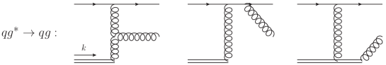
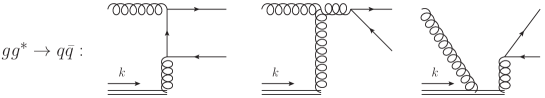
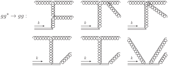
Figure 2: Diagrams contributing to the gauge invariant hard factors $\tilde{\mathcal{H}}_{ag^{*}\rightarrow bc}^{\left(i\right)}$ for various channels. We show only planar color-ordered diagrams, i.e. the planar diagrams with fixed ordering of external legs, as they are enough to reconstruct the hard factors contributing to the in-equivalent color flows (see Section 6 of (Kotko:2015ura, ) on how to reconstruct the hard factors from color-ordered amplitudes and (Mangano:1990by, ) for a general review of color decompositions). The off-shell gluon has momentum $k$. The double line corresponds to the Wilson line propagator in momentum space, which couples to gluons via the $igt^{a}P^{\mu}$ vertex. The double line propagator with a momentum $p$ is $-i/\left(p\cdot P+i\epsilon\right)$. These diagrams have to be multiplied by $\boldsymbol{k}^{2}/g$ – for all the details see Kotko2014a . We do not display the diagrams for processes with a photon since they do not require the use of a Wilson line, despite the off-shellnes of the gluon.

The form of the generalized factorization (49) appears as follows. First the color structure is separated from the kinematic part of the amplitude by means of the color decomposition (Mangano:1990by, ). The amplitudes with the color structure separated contain only planar diagrams with fixed ordering of the external legs. The TMD gluon distributions $\Phi_{ag\rightarrow bc}^{\left(i\right)}$ are derived for the color structures (squared) following the general procedure of resummation of collinear gluons constructed in (TMD, ). The color decomposition of amplitudes guarantees that each $\Phi_{ag\rightarrow bc}^{\left(i\right)}$ corresponds to a gauge invariant subset of diagrams. For more details and application to multiparticle processes see (Bury2018, ).

The iTMD formula was constructed to agree with the $k_{T}$-factorization for dijet production (Deak:2009xt, ) in the limit of $\boldsymbol{k}^{2}\sim Q^{2}\gg Q_{s}^{2}$ and also with the leading power limit of the CGC expressions (Dominguez:2011wm, ) for $Q^{2}\gg\boldsymbol{k}^{2}\sim Q_{s}^{2}$. In the present paper we further compare all the power corrections contained in the framework. To this end, we need the small $x$ limit of the TMD gluon distributions compliant with the CGC theory. They are obtained by neglecting the $x$ dependence in the Fourier transforms and trading the hadronic matrix elements to the averages over the color distributions in the nucleus. In addition, lightcone gauge is used, in which for the shockwave approximation the transverse components of the gauge fields do not contribute due to EOM. This allows to neglect the transverse parts of the staple gauge links (58). Within the above approximation we have (Dominguez:2011wm, ; Marquet:2016cgx, ):

$$\mathcal{F}_{qg}^{\left(1\right)}=\frac{4}{g^{2}}\,\int\frac{d^{2}\boldsymbol{x}d^{2}\boldsymbol{y}}{\left(2\pi\right)^{3}}\,e^{-i\boldsymbol{k}\cdot\left(\boldsymbol{x}-\boldsymbol{y}\right)}\left\langle\mathrm{Tr}\left\{\left(\partial_{i}U_{\boldsymbol{y}}\right)\left(\partial_{i}U_{\boldsymbol{x}}^{\dagger}\right)\right\}\right\rangle\,,$$ (60)

$$\mathcal{F}_{qg}^{\left(2\right)}=-\frac{4}{g^{2}}\,\int\frac{d^{2}\boldsymbol{x}d^{2}\boldsymbol{y}}{\left(2\pi\right)^{3}}\,e^{-i\boldsymbol{k}\cdot\left(\boldsymbol{x}-\boldsymbol{y}\right)}\frac{1}{N_{c}}\left\langle\mathrm{Tr}\left\{\left(\partial_{i}U_{\boldsymbol{x}}\right)U_{\boldsymbol{y}}^{\dagger}\left(\partial_{i}U_{\boldsymbol{y}}^{\dagger}\right)U_{\boldsymbol{x}}^{\dagger}\right\}\mathrm{Tr}\left\{U_{\boldsymbol{y}}U_{\boldsymbol{x}}^{\dagger}\right\}\right\rangle\,.$$ (61)

$$\mathcal{F}_{gg}^{\left(1\right)}=\frac{4}{g^{2}}\,\int\frac{d^{2}\boldsymbol{x}d^{2}\boldsymbol{y}}{\left(2\pi\right)^{3}}\,e^{-i\boldsymbol{k}\cdot\left(\boldsymbol{x}-\boldsymbol{y}\right)}\frac{1}{N_{c}}\left\langle\mathrm{Tr}\left\{\left(\partial_{i}U_{\boldsymbol{y}}\right)\left(\partial_{i}U_{\boldsymbol{x}}^{\dagger}\right)\right\}\mathrm{Tr}\left\{U_{\boldsymbol{x}}U_{\boldsymbol{y}}^{\dagger}\right\}\right\rangle\,,$$ (62)

$$\mathcal{F}_{gg}^{\left(2\right)}=-\frac{4}{g^{2}}\,\int\frac{d^{2}\boldsymbol{x}d^{2}\boldsymbol{y}}{\left(2\pi\right)^{3}}\,e^{-i\boldsymbol{k}\cdot\left(\boldsymbol{x}-\boldsymbol{y}\right)}\frac{1}{N_{c}}\left\langle\mathrm{Tr}\left\{\left(\partial_{i}U_{\boldsymbol{x}}\right)U_{\boldsymbol{y}}^{\dagger}\right\}\mathrm{Tr}\left\{\left(\partial_{i}U_{\boldsymbol{y}}\right)U_{\boldsymbol{x}}^{\dagger}\right\}\right\rangle\,,$$ (63)

$$\mathcal{F}_{gg}^{\left(3\right)}=-\frac{4}{g^{2}}\,\int\frac{d^{2}\boldsymbol{x}d^{2}\boldsymbol{y}}{\left(2\pi\right)^{3}}\,e^{-i\boldsymbol{k}\cdot\left(\boldsymbol{x}-\boldsymbol{y}\right)}\left\langle\mathrm{Tr}\left\{\left(\partial_{i}U_{\boldsymbol{x}}\right)U_{\boldsymbol{y}}^{\dagger}\left(\partial_{i}U_{\boldsymbol{y}}\right)U_{\boldsymbol{x}}^{\dagger}\right\}\right\rangle\,,$$ (64)

$$\mathcal{F}_{gg}^{\left(4\right)}=-\frac{4}{g^{2}}\,\int\frac{d^{2}\boldsymbol{x}d^{2}\boldsymbol{y}}{\left(2\pi\right)^{3}}\,e^{-i\boldsymbol{k}\cdot\left(\boldsymbol{x}-\boldsymbol{y}\right)}\left\langle\mathrm{Tr}\left\{\left(\partial_{i}U_{\boldsymbol{x}}\right)U_{\boldsymbol{x}}^{\dagger}\left(\partial_{i}U_{\boldsymbol{y}}\right)U_{\boldsymbol{y}}^{\dagger}\right\}\right\rangle\,,$$ (65)

$$\mathcal{F}_{gg}^{\left(5\right)}=-\frac{4}{g^{2}}\,\int\frac{d^{2}\boldsymbol{x}d^{2}\boldsymbol{y}}{\left(2\pi\right)^{3}}\,e^{-i\boldsymbol{k}\cdot\left(\boldsymbol{x}-\boldsymbol{y}\right)}\left\langle\mathrm{Tr}\left\{\left(\partial_{i}U_{\boldsymbol{x}}\right)U_{\boldsymbol{y}}^{\dagger}U_{\boldsymbol{x}}U_{\boldsymbol{y}}^{\dagger}\left(\partial_{i}U_{\boldsymbol{y}}\right)U_{\boldsymbol{x}}^{\dagger}U_{\boldsymbol{y}}U_{\boldsymbol{x}}^{\dagger}\right\}\right\rangle\,,$$ (66)

$$\mathcal{F}_{gg}^{\left(6\right)}=-\frac{4}{g^{2}}\,\int\frac{d^{2}\boldsymbol{x}d^{2}\boldsymbol{y}}{\left(2\pi\right)^{3}}\,e^{-i\boldsymbol{k}\cdot\left(\boldsymbol{x}-\boldsymbol{y}\right)}\\ \frac{1}{N_{c}^{2}}\left\langle\mathrm{Tr}\left\{\left(\partial_{i}U_{\boldsymbol{x}}\right)U_{\boldsymbol{y}}^{\dagger}\left(\partial_{i}U_{\boldsymbol{y}}\right)U_{\boldsymbol{x}}^{\dagger}\right\}\mathrm{Tr}\left\{U_{\boldsymbol{x}}U_{\boldsymbol{y}}^{\dagger}\right\}\mathrm{Tr}\left\{U_{\boldsymbol{y}}U_{\boldsymbol{x}}^{\dagger}\right\}\right\rangle\,.$$ (67)

For completeness, let us now put the iTMD formulation into the context of the formal TMD factorization theorems (Collins:2011zzd, ). First, one should understand that it does not involve an all-order factorization theorem like the ones existing for the Drell-Yan process and semi-inclusive DIS. These theorems are proved to leading power in the hard scale to any logarithmic accuracy, while the iTMD framework resums the power corrections, but its validity is limited to leading logarithms of energy. Next, the mentioned TMD factorization theorems involve processes with at most two colored partons in the hard process (plus soft/collinear contributions of course) and two TMD correlators (parton distribution or fragmentation function). Because of the simplicity of the color structure, all Wilson lines appearing due to the resummation of collinear gluons can be disentangled and put into the gauge invariant definitions of the TMD objects. For jet production processes in hadron-hadron collision, where formally one has at least two TMD correlators and more than two colored partons, it is not possible. Thus, formally, even the generalized factorization breaks down (Rogers:2010dm, ). However, in the iTMD approach, which targets the collisions of a moderate-$x$ projectile and a low-$x$ target, there is only one TMD correlator, thus, at least formally, this problem does not occur. On the formal ground there is no all-order proof of the hybrid approach so far.

Finally, let us comment on the evolution equations for the TMD gluon distributions. The most adequate treatment would be using the renormalization group equation at small and moderate $x$ developed in (Balitsky2015a, ; Balitsky2016, ). It however still requires work to derive the complete set of equations, not to mention solving them. An important feature of such procedure would be that some Sudakov logarithms $\ln\boldsymbol{k}^{2}$ can be consistently resummed. For existing phenomenological applications using iTMD (vanHameren:2016ftb, ; Kotko2017b, ) the evolution was based on BK or B-JIMWLK and some Sudakov resummation effects were estimated by means of a phenomenological model.

Below, we explicitly give formulas for the cross sections (49) in a form that can be directly compared with the CGC expressions.

5.2 $qg^{*}\rightarrow qg$ channel

We get

$$\frac{d\sigma_{qA\rightarrow qg}}{d^{2}\boldsymbol{p}_{1}d^{2}\boldsymbol{p}_{2}dy_{1}dy_{2}}=p_{0}^{+}\delta\left(p_{1}^{+}+p_{2}^{+}-p_{0}^{+}\right)\left[\mathcal{H}_{qg\rightarrow qg}^{\left(1\right)}\Phi_{qg\rightarrow qg}^{\left(1\right)}+\mathcal{H}_{qg\rightarrow qg}^{\left(2\right)}\Phi_{qg\rightarrow qg}^{\left(2\right)}\right]\,,$$ (68)

with

$$\mathcal{H}_{qg\rightarrow qg}^{\left(1\right)}=\alpha_{s}^{2}\,\frac{z^{2}\left(1+z^{2}\right)}{2\boldsymbol{q}^{2}}\Bigg{\{}\frac{z}{\boldsymbol{p}_{1}^{2}}+\frac{1}{N_{c}^{2}}\frac{\boldsymbol{q}^{2}-\overline{z}^{2}\boldsymbol{p}_{1}^{2}}{{z}\boldsymbol{p}_{1}^{2}\boldsymbol{p}_{2}^{2}}\Bigg{\}}\,,$$ (69)

$$\mathcal{H}_{qg\rightarrow qg}^{\left(2\right)}=\alpha_{s}^{2}\,\frac{N_{A}}{2N_{c}^{2}}\,\frac{{z}\left(1+{z}^{2}\right)}{\boldsymbol{p}_{1}^{2}\boldsymbol{p}_{2}^{2}}\,.$$ (70)

Note, that the above hard factors $\mathcal{H}_{qg\rightarrow qg}^{\left(i\right)}$ are not exactly the ones in (49). The expressions are however more compact in the above notation.

5.3 $gg^{*}\rightarrow q\overline{q}$ channel

$$\frac{d\sigma_{gA\rightarrow q\overline{q}}}{d^{2}\boldsymbol{p}_{1}d^{2}\boldsymbol{p}_{2}dy_{1}dy_{2}}=p_{0}^{+}\delta\left(p_{1}^{+}+p_{2}^{+}-p_{0}^{+}\right)\left[\mathcal{H}_{gg\rightarrow q\overline{q}}^{\left(1\right)}\Phi_{gg\rightarrow q\overline{q}}^{\left(1\right)}+\mathcal{H}_{gg\rightarrow q\overline{q}}^{\left(2\right)}\Phi_{gg\rightarrow q\overline{q}}^{\left(2\right)}\right]\,,$$ (71)

where $\mathcal{H}_{gg\rightarrow q\overline{q}}^{\left(1\right)}$, $\mathcal{H}_{gg\rightarrow q\overline{q}}^{\left(2\right)}$ are the reduced off-shell hard factors. They read

$$\mathcal{H}_{gg\rightarrow q\overline{q}}^{\left(1\right)}=\frac{\alpha_{s}^{2}}{2N_{c}}\,\,z\overline{z}\left(1-2z\overline{z}\right)\,\frac{\boldsymbol{p}_{1}^{2}\left(1-z\right)^{2}+\boldsymbol{p}_{2}^{2}z^{2}}{\boldsymbol{q}^{2}\boldsymbol{p}_{1}^{2}\boldsymbol{p}_{2}^{2}}\,,$$ (72)

$$\mathcal{H}_{gg\rightarrow q\overline{q}}^{\left(2\right)}=\frac{\alpha_{s}^{2}}{2N_{c}^{2}C_{F}}\,\left(z\overline{z}\right)^{2}\left(1-2z\overline{z}\right)\,\frac{(\boldsymbol{p_{1}}\cdot\boldsymbol{p_{2}})}{\boldsymbol{q}^{2}\boldsymbol{p}_{1}^{2}\boldsymbol{p}_{2}^{2}}\,.$$ (73)

5.4 $gg^{*}\rightarrow gg$ channel

$$\frac{d\sigma_{gA\rightarrow gg}}{d^{2}\boldsymbol{p}_{1}d^{2}\boldsymbol{p}_{2}dy_{1}dy_{2}}=p_{0}^{+}\delta\left(p_{1}^{+}+p_{2}^{+}-p_{0}^{+}\right)\left[\mathcal{H}_{gg\rightarrow gg}^{\left(1\right)}\Phi_{gg\rightarrow gg}^{\left(1\right)}+\mathcal{H}_{gg\rightarrow gg}^{\left(2\right)}\Phi_{gg\rightarrow gg}^{\left(2\right)}\right]\,,$$ (74)

with

$$\mathcal{H}_{gg\rightarrow gg}^{\left(1\right)}=\alpha_{s}^{2}\frac{2N_{c}^{2}}{N_{A}}\,\left(1-z\overline{z}\right)^{2}\,\frac{\boldsymbol{p}_{1}^{2}\overline{z}^{2}+\boldsymbol{p}_{2}^{2}z^{2}}{\boldsymbol{q}^{2}\boldsymbol{p}_{1}^{2}\boldsymbol{p}_{2}^{2}}\,,$$ (75)

$$\mathcal{H}_{gg\rightarrow gg}^{\left(2\right)}=\alpha_{s}^{2}\frac{N_{c}^{2}}{N_{A}}\,\left(1-z\overline{z}\right)^{2}\,\frac{\boldsymbol{q}^{2}-\boldsymbol{p}_{1}^{2}\overline{z}^{2}-\boldsymbol{p}_{2}^{2}z^{2}}{\boldsymbol{q}^{2}\boldsymbol{p}_{1}^{2}\boldsymbol{p}_{2}^{2}}\,.$$ (76)

Above, an additional symmetry factor of $1/2$ was included to account for identical final states.

5.5 $\gamma g^{*}\rightarrow q\overline{q}$ channel

$$\frac{d\sigma_{\gamma A\rightarrow q\overline{q}}}{d^{2}\boldsymbol{p}_{1}d^{2}\boldsymbol{p}_{2}dy_{1}dy_{2}}=p_{0}^{+}\delta\left(p_{1}^{+}+p_{2}^{+}-p_{0}^{+}\right)\mathcal{H}_{\gamma g^{*}\rightarrow gg}\mathcal{F}_{gg}^{\left(3\right)}\,,$$ (77)

with

$$\mathcal{H}_{\gamma g^{*}\rightarrow gg}=\alpha_{\mathrm{em}}\alpha_{s}\,\frac{z\overline{z}\left(1-2z\overline{z}\right)}{\boldsymbol{p}_{1}^{2}\boldsymbol{p}_{2}^{2}}\,.$$ (78)

5.6 $qg^{*}\rightarrow q\gamma$ channel

$$\frac{d\sigma_{qA\rightarrow q\gamma}}{d^{2}\boldsymbol{p}_{1}d^{2}\boldsymbol{p}_{2}dy_{1}dy_{2}}=p_{0}^{+}\delta\left(p_{1}^{+}+p_{2}^{+}-p_{0}^{+}\right)\mathcal{H}_{qg^{*}\rightarrow q\gamma}\mathcal{F}_{qg}^{\left(1\right)}\,,$$ (79)

with

$$\mathcal{H}_{qg^{*}\rightarrow q\gamma}=\alpha_{\mathrm{em}}\alpha_{s}\,\frac{1}{C_{A}}\,\frac{z\overline{z}^{2}\left(1+z^{2}\right)}{\boldsymbol{q}^{2}\boldsymbol{p}_{2}^{2}}\,.$$ (80)

6 From the generic CGC process to the specific cases

In sections 3 and 4, we have computed both the kinematic-twist-resummed cross section and the dilute limit of the CGC cross section for a generic $1\to 2$ process respectively. Our aim in this section is to get both of these cross sections for specific processes and compare these results with the ones that are obtained through iTMD framework in section 5.

To be more accurate, we consider the photoproduction of a dijet, as well as all possible channels for two particle production (dijet or photon-jet) in forward pp and pA collisions. Within the CGC framework, hybrid formalism Dumitru:2005gt is the state of the art approach for these processes. It has been very successfully used to calculate the next-to-leading order single inclusive particle production Altinoluk:2011qy -Ducloue:2017mpb , heavy quark production Altinoluk:2015vax , dijet production Marquet:2016cgx and recently dijet+photon Altinoluk:2018byz ; Altinoluk:2018uax and trijet production Iancu:2018hwa in forward pA collisions.

In the hybrid formalism, the final state particles are produced in the forward rapidity region so they can be treated in the collinear framework, i.e. the incoming partons are on-shell collinear partons and the partonic cross section calculated in this set up should be convoluted with the collinear parton distribution functions in order to get the hadronic cross sections. On the other hand, the target is assumed to be dense and the center-of-mass energy is large so it can be treated in the CGC framework. At the parton level, the set up that we have used for the calculation of the kinematic-twist-resummed cross section Eq. (39) and the dilute cross section Eq. (47) for a generic process is compatible with the hybrid formalism. Thus, we use those results to study the different channels and compare them with the ones obtained from iTMD framework in the rest of this section.

6.1 $q\rightarrow qg$ channel

Let us start our analysis by considering the $q\rightarrow qg$ channel (see Fig. 3). In this channel, the incoming quark splits into a quark-gluon pair at order $g_{s}$ which then scatters off the target via eikonal interaction. The CGC amplitude for this channel is given in Eq. (132). In order to be able to use the kinematic twist resummed generic cross section Eq. (39), the first thing we need is the tensor part of the amplitude that encodes the Dirac structure of this channel and it is given by

$$\phi_{\mu}^{\left(q\rightarrow qg\right)} =\frac{ig_{s}}{2\pi}\varepsilon_{p_{g}\perp}^{\sigma\ast}\bar{u}_{p_{q}}\left[2zg_{\perp\mu\sigma}+\bar{z}\left(\gamma_{\perp\mu}\gamma_{\perp\sigma}\right)\right]\gamma^{+}u_{p},$$ (81)

whose square for an unpolarized observable can be calculated in a straightforward manner and the result reads

$$\phi^{i\left(q\rightarrow qg\right)}\phi^{i^{\prime}\ast\left(q\rightarrow qg\right)} =\delta^{ii^{\prime}}\left(\frac{g_{s}}{2\pi}\right)^{2}\left(p_{0}^{+}\right)^{2}16z\left(1+z^{2}\right).$$ (82)

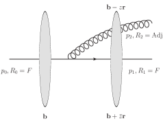
Figure 3: $q\to qg$ amplitude in an external shockwave background with the appropriate color representations.

One can read off the color structure in this channel from Fig. 3 and it is given by setting $U_{\boldsymbol{b}}^{R_{1}}=U_{\boldsymbol{b}},$ $U_{\boldsymbol{b}}^{R_{2}}=U_{\boldsymbol{b}}^{ab}$ and $T^{R_{0}}=T^{b}$. This color structure leads to the following TMD operators

$$\mathcal{O}_{1}^{\left(q\rightarrow qg\right)} =\left(\partial^{j}U_{\boldsymbol{b}}\right)T^{b}U_{\boldsymbol{b}}^{ab}U_{\boldsymbol{b}^{\prime}}^{ac\dagger}T^{c}\left(\partial^{j^{\prime}}U_{\boldsymbol{b}^{\prime}}^{\dagger}\right)$$

$$\mathcal{O}_{2}^{\left(q\rightarrow qg\right)} =\left(\partial^{j}U_{\boldsymbol{b}}\right)T^{b}U_{\boldsymbol{b}}^{ab}\left(\partial^{j^{\prime}}U_{\boldsymbol{b}^{\prime}}^{ac}\right)T^{c}U_{\boldsymbol{b}^{\prime}}^{\dagger}$$ (83)

$$\mathcal{O}_{3}^{\left(q\rightarrow qg\right)} =U_{\boldsymbol{b}}T^{b}\left(\partial^{j}U_{\boldsymbol{b}}^{ab}\right)U_{\boldsymbol{b}^{\prime}}^{ac\dagger}T^{c}\left(\partial^{j^{\prime}}U_{\boldsymbol{b}^{\prime}}^{\dagger}\right)$$

$$\mathcal{O}_{4}^{\left(q\rightarrow qg\right)} =U_{\boldsymbol{b}}T^{b}\left(\partial^{j}U_{\boldsymbol{b}}^{ab}\right)\left(\partial^{j^{\prime}}U_{\boldsymbol{b}^{\prime}}^{ac}\right)T^{c}U_{\boldsymbol{b}^{\prime}}^{\dagger}.$$

By using the identity that relates the adjoint and fundamental representations of a unitary matrix

$$U^{ab}(\boldsymbol{b})=2\,\mathrm{Tr}\big{[}t^{a}U(\boldsymbol{b})t^{b}U^{\dagger}(\boldsymbol{b})\big{]}$$ (84)

and the Fierz identity

$$t^{a}_{\alpha\beta}t^{a}_{\sigma\lambda}=\frac{1}{2}\bigg{[}\delta_{\alpha\lambda}\delta_{\beta\sigma}-\frac{1}{N_{c}}\delta_{\alpha\beta}\delta_{\sigma\lambda}\bigg{]}$$ (85)

one can easily get the following identities

$$T^{b}\left(\partial^{j}U_{\boldsymbol{b}}^{ab}\right) =\left(\partial^{j}U_{\boldsymbol{b}}^{\dagger}\right)T^{a}U_{\boldsymbol{b}}+U_{\boldsymbol{b}}^{\dagger}T^{a}\left(\partial^{j}U_{\boldsymbol{b}}\right)$$ (86)

$$\left(\partial^{j^{\prime}}U_{\boldsymbol{b}^{\prime}}^{ac}\right)T^{c\dagger} =\left(\partial^{j^{\prime}}U_{\boldsymbol{b}^{\prime}}^{\dagger}\right)T^{a}U_{\boldsymbol{b}^{\prime}}+U_{\boldsymbol{b}^{\prime}}^{\dagger}T^{a}\left(\partial^{j^{\prime}}U_{\boldsymbol{b}^{\prime}}\right),$$

The next step is to compute the color trace of the TMD operators that are listed in Eq. (83). By using the identities given in Eq. (86), these traces can easily be computed and the result reads

$$\mathrm{Tr}\,\Big{[}\mathcal{O}_{1}^{\left(q\rightarrow qg\right)}\Big{]} =-\frac{1}{2}\mathrm{Tr}\left[\left(\partial^{j}U_{\boldsymbol{b}}\right)U_{\boldsymbol{b}}^{\dagger}\left(\partial^{j^{\prime}}U_{\boldsymbol{b}^{\prime}}\right)U_{\boldsymbol{b}^{\prime}}^{\dagger}\right]\mathrm{Tr}\left(U_{\boldsymbol{b}}U_{\boldsymbol{b}^{\prime}}^{\dagger}\right)-\frac{1}{2N_{c}}\mathrm{Tr}\left[\left(\partial^{j}U_{\boldsymbol{b}}\right)\left(\partial^{j^{\prime}}U_{\boldsymbol{b}^{\prime}}^{\dagger}\right)\right]$$

$$\mathrm{Tr}\,\Big{[}\mathcal{O}_{2}^{\left(q\rightarrow qg\right)}\Big{]} =\frac{1}{2}\mathrm{Tr}\left[\left(\partial^{j}U_{\boldsymbol{b}}\right)U_{\boldsymbol{b}}^{\dagger}\left(\partial^{j^{\prime}}U_{\boldsymbol{b}^{\prime}}\right)U_{\boldsymbol{b}^{\prime}}^{\dagger}\right]\mathrm{Tr}\left(U_{\boldsymbol{b}}U_{\boldsymbol{b}^{\prime}}^{\dagger}\right)$$ (87)

$$\mathrm{Tr}\,\Big{[}\mathcal{O}_{3}^{\left(q\rightarrow qg\right)}\Big{]} =\frac{1}{2}\mathrm{Tr}\left[\left(\partial^{j}U_{\boldsymbol{b}}\right)U_{\boldsymbol{b}}^{\dagger}\left(\partial^{j^{\prime}}U_{\boldsymbol{b}^{\prime}}\right)U_{\boldsymbol{b}^{\prime}}^{\dagger}\right]\mathrm{Tr}\left(U_{\boldsymbol{b}}U_{\boldsymbol{b}^{\prime}}^{\dagger}\right)$$

$$\mathrm{Tr}\,\Big{[}\mathcal{O}_{4}^{\left(q\rightarrow qg\right)}\Big{]} =-\frac{1}{2}\mathrm{Tr}\left[\left(\partial^{j}U_{\boldsymbol{b}}\right)U_{\boldsymbol{b}}^{\dagger}\left(\partial^{j^{\prime}}U_{\boldsymbol{b}^{\prime}}\right)U_{\boldsymbol{b}^{\prime}}^{\dagger}\right]\mathrm{Tr}\left(U_{\boldsymbol{b}}U_{\boldsymbol{b}^{\prime}}^{\dagger}\right)+\frac{N_{c}}{2}\mathrm{Tr}\left[\left(\partial^{j}U_{\boldsymbol{b}}\right)\left(\partial^{j^{\prime}}U_{\boldsymbol{b}^{\prime}}^{\dagger}\right)\right].$$

Comparing the structure of the trace of the Wilson lines in Eq. (87) and the definitions of the first two gluon TMDs in the quark channel $\mathcal{F}_{qg}^{\left(1\right)}$ and $\mathcal{F}_{qg}^{\left(2\right)}$ given in Eqs. (60) and (61) respectively, one can conclude that these are the two gluon TMDs which appear in this channel. Moreover, for convenience, we can define the following combinations of the gluon TMDs $\mathcal{F}_{qg}^{\left(1\right)}$ and $\mathcal{F}_{qg}^{\left(2\right)}$ :

$$\Phi_{q\rightarrow qg}^{\left(1\right)}\left(\boldsymbol{k}\right) \equiv\mathcal{F}_{qg}^{\left(1\right)}\left(\boldsymbol{k}\right)$$ (88)

$$\Phi_{q\rightarrow qg}^{\left(2\right)}\left(\boldsymbol{k}\right) \equiv\frac{N_{c}^{2}\mathcal{F}_{qg}^{\left(2\right)}\left(\boldsymbol{k}\right)-\mathcal{F}_{qg}^{\left(1\right)}\left(\boldsymbol{k}\right)}{N_{c}^{2}-1}$$

which are exactly the same combinations that one gets from the iTMD calculations given in the Table 1.

Finally, we can plug the square of the tensor part of the amplitude given in Eq. (82) and the Wilson line structure given in Eq. (87) together with the definitions and the combinations of the gluon TMDs Eq. (88) in the generic kinematic twist resummed cross section Eq. (39) to get the cross section for $q\to qg$ channel as

$$\frac{d\sigma_{q\rightarrow qg}^{WW}}{dy_{1}dy_{2}d^{2}\boldsymbol{p}_{1}d^{2}\boldsymbol{p}_{2}} =\alpha_{s}^{2}\frac{z\left(1+z^{2}\right)}{2\boldsymbol{p}_{1}^{2}\boldsymbol{p}_{2}^{2}}p_{0}^{+}\delta\left(p_{1}^{+}+p_{2}^{+}-p_{0}^{+}\right)$$ (89)

$$\times\left[\left(z^{2}\frac{\boldsymbol{p}_{2}^{2}}{\boldsymbol{q}^{2}}+\frac{1}{N_{c}^{2}}\left(1-\bar{z}^{2}\frac{\boldsymbol{p}_{1}^{2}}{\boldsymbol{q}^{2}}\right)\right)\Phi_{q\rightarrow qg}^{\left(1\right)}\left(\boldsymbol{k}\right)+\left(\frac{N_{c}^{2}-1}{N_{c}^{2}}\right)\Phi_{q\rightarrow qg}^{\left(2\right)}\left(\boldsymbol{k}\right)\right]$$

which coincides exactly with Eq. (68) by using Eqs. (69) and (70).

Our next order of business is to consider the dilute limit in the $q\to qg$ channel. Inserting the proper color representations in the dilute limit of the generic cross section given in Eq. (47), we get

$$\frac{d\sigma_{q\rightarrow qg}^{gA\sim 0}}{dy_{1}dy_{2}d^{2}\boldsymbol{p}_{1}d^{2}\boldsymbol{p}_{2}}=\frac{\alpha_{s}}{16N_{c}\left(p_{0}^{+}\right)^{2}}\left(2\pi\right)\frac{\mathcal{G}_{ac}\left(\boldsymbol{k}\right)}{\boldsymbol{k}^{2}}\left(\phi^{i}\phi^{j\ast}\right)p_{0}^{+}\delta\left(p_{1}^{+}+p_{2}^{+}-p_{0}^{+}\right)$$ (90)

$$\times\mathrm{Tr}\left[if^{bad}t^{d}\left(\frac{\boldsymbol{p}_{1}^{i}}{\boldsymbol{p}_{1}^{2}}-\frac{\boldsymbol{q}^{i}}{\boldsymbol{q}^{2}}\right)-t^{a}t^{b}\left(\frac{\boldsymbol{p}_{2}^{i}}{\boldsymbol{p}_{2}^{2}}+\frac{\boldsymbol{q}^{i}}{\boldsymbol{q}^{2}}\right)\right]\left[-if^{bce}t^{e}\left(\frac{\boldsymbol{p}_{1}^{j}}{\boldsymbol{p}_{1}^{2}}-\frac{\boldsymbol{q}^{j}}{\boldsymbol{q}^{2}}\right)-t^{b}t^{c}\left(\frac{\boldsymbol{p}_{2}^{j}}{\boldsymbol{p}_{2}^{2}}+\frac{\boldsymbol{q}^{j}}{\boldsymbol{q}^{2}}\right)\right],$$

with $\mathcal{G}_{ac}\left(\boldsymbol{k}\right)$ being the unintegrated parton distribution function defined in Eq. (46). Using the definition of the tensor part of the amplitude that encodes the Dirac structure in the $q\to qg$ channel given in Eq. (81) and performing some color algebra, one simply gets the dilute limit of the cross section in this channel:

$$\frac{d\sigma_{q\rightarrow qg}^{gA\sim 0}}{dy_{1}dy_{2}d^{2}\boldsymbol{p}_{1}d^{2}\boldsymbol{p}_{2}} =\alpha_{s}^{2}\frac{z\left(1+z^{2}\right)}{2\boldsymbol{p}_{1}^{2}\boldsymbol{p}_{2}^{2}}p_{0}^{+}\delta\left(p_{1}^{+}+p_{2}^{+}-p_{0}^{+}\right)\mathcal{G}\left(\boldsymbol{k}\right)\left(1+z^{2}\frac{\boldsymbol{p}_{2}^{2}}{\boldsymbol{q}^{2}}-\frac{1}{N_{c}^{2}}\frac{\bar{z}^{2}\boldsymbol{p}_{1}^{2}}{\boldsymbol{q}^{2}}\right).$$ (91)

From Eq. (89) and (91), we also get a straightforward matching between the improved TMD scheme and the dilute scheme:

$$\sigma_{q\rightarrow qg}^{gA\sim 0}=\left.\sigma_{q\rightarrow qg}^{WW}\right|_{\Phi_{q\rightarrow qg}^{\left(1\right)}=\Phi_{q\rightarrow qg}^{\left(2\right)}=\mathcal{G}}.$$ (92)

The substitution $\Phi_{q\rightarrow qg}^{\left(1\right)}=\Phi_{q\rightarrow qg}^{\left(2\right)}=\mathcal{G}$ in the iTMD scheme in the dilute limit can be simply justified as follows. For $|\boldsymbol{k}|\gg Q_{s}$ and large, the Fourier transforms in the operator definitions force the transverse separation between the fields to be small. In that limit the gauge links become identical, while the Wilson loops become trivial. This universal behaviour was tested numerically in vanHameren:2016ftb and Marquet:2016cgx .

6.2 $g\rightarrow q\bar{q}$ channel

The next channel we consider is $g\to q\bar{q}$. In this channel, the incoming gluon splits into a quark-antiquark pair at order $g_{s}$, then it scatters through the target (see Fig. 4). The CGC amplitude for this channel is given in Eq. (133) and the tensor part of it reads

$$\phi_{\mu}^{\left(g\rightarrow q\bar{q}\right)} =-i\frac{g_{s}}{2\pi}\varepsilon_{p\perp}^{\sigma}\bar{u}_{p_{q}}\left[2zg_{\perp\mu\sigma}-\left(\gamma_{\perp\mu}\gamma_{\perp\sigma}\right)\right]\gamma^{+}v_{p_{\bar{q}}},$$ (93)

whose square can be computed easily for an unpolarized observable:

$$\phi^{i\left(g\rightarrow q\bar{q}\right)}\phi^{i^{\prime}\ast\left(g\rightarrow q\bar{q}\right)} =\delta^{ii^{\prime}}\left(\frac{g_{s}}{2\pi}\right)^{2}\left(p_{0}^{+}\right)^{2}16z\bar{z}\left(z^{2}+\bar{z}^{2}\right)$$ (94)

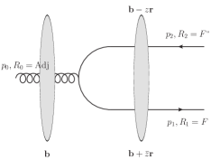
Figure 4: $g\to q\bar{q}$ amplitude in an external shockwave background with the appropriate color representations.

The color structure of this channel can be read off from Fig. 4 and it is given by setting $U_{\boldsymbol{b}}^{R_{1}}=U_{\boldsymbol{b}},$ $U_{\boldsymbol{b}}^{R_{2}}=U_{\boldsymbol{b}}^{\dagger}$ and $T^{R_{0}}=T^{b}$. This color structure leads to the following gluon TMD operators that appears in the generic kinematic twist resummed cross section given in Eq. (39):

$$\mathcal{O}_{1}^{\left(g\rightarrow q\bar{q}\right)} = \left(\partial^{j}U_{\boldsymbol{b}}\right)T^{b}U_{\boldsymbol{b}}^{\dagger}U_{\boldsymbol{b}^{\prime}}T^{b}\left(\partial^{j^{\prime}}U_{\boldsymbol{b}^{\prime}}^{\dagger}\right)$$

$$\mathcal{O}_{2}^{\left(g\rightarrow q\bar{q}\right)} = \left(\partial^{j}U_{\boldsymbol{b}}\right)T^{R}U_{\boldsymbol{b}}^{\dagger}\left(\partial^{j^{\prime}}U_{\boldsymbol{b}^{\prime}}\right)T^{b}U_{\boldsymbol{b}^{\prime}}$$ (95)

$$\mathcal{O}_{3}^{\left(g\rightarrow q\bar{q}\right)} = U_{\boldsymbol{b}}T^{b}\left(\partial^{j}U_{\boldsymbol{b}}^{\dagger}\right)U_{\boldsymbol{b}^{\prime}}T^{b}\left(\partial^{j^{\prime}}U_{\boldsymbol{b}^{\prime}}^{\dagger}\right)$$

$$\mathcal{O}_{4}^{\left(g\rightarrow q\bar{q}\right)} = U_{\boldsymbol{b}}T^{b}\left(\partial^{j}U_{\boldsymbol{b}}^{\dagger}\right)\left(\partial^{j^{\prime}}U_{\boldsymbol{b}^{\prime}}\right)T^{b}U_{\boldsymbol{b}^{\prime}}^{\dagger}$$

One can easily compute the trace over the color indexes of the operators listed in Eq. (95) and the result reads

$$\mathrm{Tr}\,\Big{[}\mathcal{O}_{1}^{\left(g\rightarrow q\bar{q}\right)}\Big{]} =\frac{1}{2}\mathrm{Tr}\left[\left(\partial^{j}U_{\boldsymbol{b}}\right)\left(\partial^{j^{\prime}}U_{\boldsymbol{b}^{\prime}}^{\dagger}\right)\right]\mathrm{Tr}\left(U_{\boldsymbol{b}^{\prime}}U_{\boldsymbol{b}}^{\dagger}\right)+\frac{1}{2N_{c}}\mathrm{Tr}\left[\left(\partial^{j}U_{\boldsymbol{b}}\right)U_{\boldsymbol{b}}^{\dagger}\left(\partial^{j^{\prime}}U_{\boldsymbol{b}^{\prime}}\right)U_{\boldsymbol{b}^{\prime}}^{\dagger}\right]$$

$$\mathrm{Tr}\,\Big{[}\mathcal{O}_{2}^{\left(g\rightarrow q\bar{q}\right)}\Big{]} =\frac{1}{2}\mathrm{Tr}\left[\left(\partial^{j}U_{\boldsymbol{b}}\right)U_{\boldsymbol{b}^{\prime}}^{\dagger}\right]\mathrm{Tr}\left[U_{\boldsymbol{b}}^{\dagger}\left(\partial^{j^{\prime}}U_{\boldsymbol{b}^{\prime}}\right)\right]-\frac{1}{2N_{c}}\mathrm{Tr}\left[\left(\partial^{j}U_{\boldsymbol{b}}\right)U_{\boldsymbol{b}}^{\dagger}\left(\partial^{j^{\prime}}U_{\boldsymbol{b}^{\prime}}\right)U_{\boldsymbol{b}^{\prime}}^{\dagger}\right]$$ (96)

$$\mathrm{Tr}\,\Big{[}\mathcal{O}_{3}^{\left(g\rightarrow q\bar{q}\right)}\Big{]} =\frac{1}{2}\mathrm{Tr}\left[\left(\partial^{j}U_{\boldsymbol{b}}^{\dagger}\right)U_{\boldsymbol{b}^{\prime}}\right]\mathrm{Tr}\left[U_{\boldsymbol{b}}\left(\partial^{j^{\prime}}U_{\boldsymbol{b}^{\prime}}^{\dagger}\right)\right]-\frac{1}{2N_{c}}\mathrm{Tr}\left[\left(\partial^{j}U_{\boldsymbol{b}}\right)U_{\boldsymbol{b}}^{\dagger}\left(\partial^{j^{\prime}}U_{\boldsymbol{b}^{\prime}}\right)U_{\boldsymbol{b}^{\prime}}^{\dagger}\right]$$

$$\mathrm{Tr}\,\Big{[}\mathcal{O}_{4}^{\left(g\rightarrow q\bar{q}\right)}\Big{]} =\frac{1}{2}\mathrm{Tr}\left[\left(\partial^{j^{\prime}}U_{\boldsymbol{b}^{\prime}}\right)\left(\partial^{j}U_{\boldsymbol{b}}^{\dagger}\right)\right]\mathrm{Tr}\left(U_{\boldsymbol{b}}U_{\boldsymbol{b}^{\prime}}^{\dagger}\right)+\frac{1}{2N_{c}}\mathrm{Tr}\left[\left(\partial^{j}U_{\boldsymbol{b}}\right)U_{\boldsymbol{b}}^{\dagger}\left(\partial^{j^{\prime}}U_{\boldsymbol{b}^{\prime}}\right)U_{\boldsymbol{b}^{\prime}}^{\dagger}\right].$$

A comparison between the Wilson line structure in this channel given in Eq. (96) and the definitions of the first three gluon TMDs in the gluon channel $\mathcal{F}_{gg}^{\left(1\right)}$, $\mathcal{F}_{gg}^{\left(2\right)}$ and $\mathcal{F}_{gg}^{\left(3\right)}$ given in Eqs. (62), (63) and (64) suggests that these are the three gluon TMDs that appear in the $g\to q\bar{q}$ channel. We define the following combinations of the TMDs which are the same combinations defined in Table 1:

$$\Phi_{g\rightarrow q\bar{q}}^{\left(1\right)}\left(\boldsymbol{k}\right) \equiv\frac{N_{c}^{2}\mathcal{F}_{gg}^{\left(1\right)}\left(\boldsymbol{k}\right)-\mathcal{F}_{gg}^{\left(3\right)}\left(\boldsymbol{k}\right)}{N_{c}^{2}-1}$$ (97)

$$\Phi_{g\rightarrow q\bar{q}}^{\left(2\right)}\left(\boldsymbol{k}\right) \equiv-N_{c}^{2}\mathcal{F}_{gg}^{\left(2\right)}\left(\boldsymbol{k}\right)+\mathcal{F}_{gg}^{\left(3\right)}\left(\boldsymbol{k}\right)$$

Finally, the square of the tensor structure, Eq. (94), the Wilson line structure, Eq. (96), and the TMD definitions with the combinations given in Eq. (97) are plugged in the generic kinematic twist resummed cross section given in Eq. (39). The result can simply be written as

$$\frac{d\sigma_{g\rightarrow q\bar{q}}^{WW}}{dy_{1}dy_{2}d^{2}\boldsymbol{p}_{1}d^{2}\boldsymbol{p}_{2}}= \frac{\alpha_{s}^{2}}{2N_{c}}p_{0}^{+}\delta\left(p_{1}^{+}+p_{2}^{+}-p_{0}^{+}\right)\frac{z\bar{z}\left(z^{2}+\bar{z}^{2}\right)}{\boldsymbol{q}^{2}}$$ (98)

$$\times\left[\frac{\bar{z}^{2}}{\boldsymbol{p}_{2}^{2}}\Phi_{g\rightarrow q\bar{q}}^{\left(1\right)}\left(\boldsymbol{k}\right)+\frac{z^{2}}{\boldsymbol{p}_{1}^{2}}\Phi_{g\rightarrow q\bar{q}}^{\left(1\right)}\left(-\boldsymbol{k}\right)+z\bar{z}\frac{\left(\boldsymbol{p}_{1}\cdot\boldsymbol{p}_{2}\right)}{\boldsymbol{p}_{1}^{2}\boldsymbol{p}_{2}^{2}}\frac{\Phi_{g\rightarrow q\bar{q}}^{\left(2\right)}\left(\boldsymbol{k}\right)+\Phi_{g\rightarrow q\bar{q}}^{\left(2\right)}\left(-\boldsymbol{k}\right)}{\left(N_{c}^{2}-1\right)}\right]$$

which coincides exactly with Eq. (71) by using Eqs. (72) and (73).

The next step is to consider the dilute limit in the $g\to q\bar{q}$ channel. Introducing the proper color structure in the generic dilute cross section in Eq. (47), we get

$$\frac{d\sigma_{g\rightarrow q\bar{q}}^{gA\sim 0}}{dy_{1}dy_{2}d^{2}\boldsymbol{p}_{1}d^{2}\boldsymbol{p}_{2}} =\frac{\alpha_{s}}{16\left(N_{c}^{2}-1\right)\left(p_{0}^{+}\right)^{2}}\left(2\pi\right)p_{0}^{+}\delta\left(p_{1}^{+}+p_{2}^{+}-p_{0}^{+}\right)\frac{\mathcal{G}_{ac}\left(\boldsymbol{k}\right)}{\boldsymbol{k}^{2}}\left(\phi^{i}\phi^{j\ast}\right)$$ (99)

$$\times\mathrm{Tr}\left[t^{b}t^{a}\left(\frac{\boldsymbol{p}_{1}^{i}}{\boldsymbol{p}_{1}^{2}}-\frac{\boldsymbol{q}^{i}}{\boldsymbol{q}^{2}}\right)+t^{a}t^{b}\left(\frac{\boldsymbol{p}_{2}^{i}}{\boldsymbol{p}_{2}^{2}}+\frac{\boldsymbol{q}^{i}}{\boldsymbol{q}^{2}}\right)\right]\left[t^{c}t^{b}\left(\frac{\boldsymbol{p}_{1}^{j}}{\boldsymbol{p}_{1}^{2}}-\frac{\boldsymbol{q}^{j}}{\boldsymbol{q}^{2}}\right)+t^{b}t^{c}\left(\frac{\boldsymbol{p}_{2}^{j}}{\boldsymbol{p}_{2}^{2}}+\frac{\boldsymbol{q}^{j}}{\boldsymbol{q}^{2}}\right)\right],$$

which after some color algebra leads to

$$\frac{d\sigma_{g\rightarrow q\bar{q}}^{gA\sim 0}}{dy_{1}dy_{2}d^{2}\boldsymbol{p}_{1}d^{2}\boldsymbol{p}_{2}} =\frac{\alpha_{s}^{2}}{N_{c}\left(N_{c}^{2}-1\right)}\frac{z\bar{z}\left(z^{2}+\bar{z}^{2}\right)}{2\boldsymbol{p}_{1}^{2}\boldsymbol{p}_{2}^{2}}p_{0}^{+}\delta\left(p_{1}^{+}+p_{2}^{+}-p_{0}^{+}\right)\mathcal{G}\left(\boldsymbol{k}\right)$$

$$\times\,\left[N_{c}^{2}\left(z^{2}\frac{\boldsymbol{p}_{2}^{2}}{\boldsymbol{q}^{2}}+\bar{z}^{2}\frac{\boldsymbol{p}_{1}^{2}}{\boldsymbol{q}^{2}}\right)-1\right].$$ (100)

Finally, a comparison between the kinematic twist resummed cross section Eq. (98) and the dilute limit of the cross section given in Eq. (100), again leads to a straightforward matching between the iTMD scheme and the dilute scheme for $g\to q\bar{q}$ channel:

$$\sigma_{g\rightarrow q\bar{q}}^{gA\sim 0}=\left.\sigma_{g\rightarrow q\bar{q}}^{WW}\right|_{\Phi_{g\rightarrow q\bar{q}}^{\left(1\right)}=\Phi_{g\rightarrow q\bar{q}}^{\left(2\right)}=\mathcal{G}}.$$ (101)

6.3 $g\rightarrow gg$ channel

The next channel we consider is $g\to gg$. The CGC amplitude for this channel is given in Eq. (134). The tensor part for this channel can simply be read off from Eq. (134) and it is given as

$$\phi_{\mu}^{\left(g\rightarrow gg\right)} =\frac{2g_{s}p_{0}^{+}}{\pi}\varepsilon_{p\perp}^{\sigma_{0}}\varepsilon_{p_{g}\perp}^{\sigma_{1}\ast}\varepsilon_{q_{g}\perp}^{\sigma_{2}\ast}\left[zg_{\perp\sigma_{0}\sigma_{1}}g_{\perp\mu\sigma_{2}}-z\bar{z}g_{\perp\sigma_{1}\sigma_{2}}g_{\perp\mu\sigma_{0}}+\bar{z}g_{\perp\sigma_{0}\sigma_{2}}g_{\perp\mu\sigma_{1}}\right]$$ (102)

Its square can be computed in a straightforward manner with the result being

$$\phi^{i\left(g\rightarrow gg\right)}\phi^{i^{\prime}\ast\left(g\rightarrow gg\right)} =\delta^{ii^{\prime}}\left(\frac{g_{s}}{2\pi}\right)^{2}\left(p_{0}^{+}\right)^{2}32\left(1-z\bar{z}\right)^{2}$$ (103)

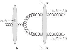
Figure 5: $g\to gg$ amplitude in an external shockwave background with the appropriate color representations.

The color structure of this channel is demonstrated in Fig. 5 and it is given by $U_{\boldsymbol{b}}^{R_{1}}=U_{\boldsymbol{b}}^{b_{1}a_{1}},$ $U_{\boldsymbol{b}}^{R_{2}}=U_{\boldsymbol{b}}^{b_{2}a_{2}}$ and $T^{R_{0}}=f^{a_{0}b_{1}b_{2}}$. This leads to the following TMD operators once it is inserted to the Wilson line structure of the generic kinematic twist resummed cross section in Eq. (39):

$$\mathcal{O}_{1}^{\left(g\rightarrow gg\right)} =\left(\partial^{j}U_{\boldsymbol{b}}^{b_{1}a_{1}}\right)f^{a_{0}b_{1}b_{2}}U_{\boldsymbol{b}}^{b_{2}a_{2}}U_{\boldsymbol{b}^{\prime}}^{a_{2}c_{2}}f^{a_{0}c_{1}c_{2}}\left(\partial^{j^{\prime}}U_{\boldsymbol{b}^{\prime}}^{a_{1}c_{1}}\right)$$

$$\mathcal{O}_{2}^{\left(g\rightarrow gg\right)} =\left(\partial^{j}U_{\boldsymbol{b}}^{b_{1}a_{1}}\right)f^{a_{0}b_{1}b_{2}}U_{\boldsymbol{b}}^{b_{2}a_{2}}\left(\partial^{j^{\prime}}U_{\boldsymbol{b}^{\prime}}^{a_{2}c_{2}}\right)f^{a_{0}c_{1}c_{2}}U_{\boldsymbol{b}^{\prime}}^{a_{1}c_{1}}$$ (104)

$$\mathcal{O}_{3}^{\left(g\rightarrow gg\right)} =U_{\boldsymbol{b}}^{b_{1}a_{1}}f^{a_{0}b_{1}b_{2}}\left(\partial^{j}U_{\boldsymbol{b}}^{b_{2}a_{2}}\right)U_{\boldsymbol{b}^{\prime}}^{a_{2}c_{2}}f^{a_{0}c_{1}c_{2}}\left(\partial^{j^{\prime}}U_{\boldsymbol{b}^{\prime}}^{a_{1}c_{1}}\right)$$

$$\mathcal{O}_{4}^{\left(g\rightarrow gg\right)} =U_{\boldsymbol{b}}^{b_{1}a_{1}}f^{a_{0}b_{1}b_{2}}\left(\partial^{j}U_{\boldsymbol{b}}^{b_{2}a_{2}}\right)\left(\partial^{j^{\prime}}U_{\boldsymbol{b}^{\prime}}^{a_{2}c_{2}}\right)f^{a_{0}c_{1}c_{2}}U_{\boldsymbol{b}^{\prime}}^{a_{1}c_{1}}.$$

After a standard but cumbersome color algebra, the trace over the color indexes of the above TMD operators can be written in terms of the fundamental Wilson line operators as

$$\mathrm{Tr}\,\Big{[}\mathcal{O}_{1}^{\left(g\rightarrow gg\right)}\Big{]} =-\mathrm{Tr}\left[\left(\partial^{j}U_{\boldsymbol{b}}\right)U_{\boldsymbol{b}}^{\dagger}\left(\partial^{j^{\prime}}U_{\boldsymbol{b}^{\prime}}\right)U_{\boldsymbol{b}^{\prime}}^{\dagger}\right]\mathrm{Tr}\left(U_{\boldsymbol{b}}U_{\boldsymbol{b}^{\prime}}^{\dagger}\right)\mathrm{Tr}\left(U_{\boldsymbol{b}^{\prime}}U_{\boldsymbol{b}}^{\dagger}\right)$$

$$-\mathrm{Tr}\left[\left(\partial^{j}U_{\boldsymbol{b}}\right)U_{\boldsymbol{b}}^{\dagger}U_{\boldsymbol{b}^{\prime}}U_{\boldsymbol{b}}^{\dagger}\left(\partial^{j^{\prime}}U_{\boldsymbol{b}^{\prime}}\right)U_{\boldsymbol{b}^{\prime}}^{\dagger}U_{\boldsymbol{b}}U_{\boldsymbol{b}^{\prime}}^{\dagger}\right]$$

$$+2\mathrm{Tr}\left[\left(\partial^{j}U_{\boldsymbol{b}}\right)U_{\boldsymbol{b}}^{\dagger}\left(\partial^{j^{\prime}}U_{\boldsymbol{b}^{\prime}}\right)U_{\boldsymbol{b}^{\prime}}^{\dagger}\right]-\mathrm{Tr}\left[\left(\partial^{j}U_{\boldsymbol{b}}^{\dagger}\right)U_{\boldsymbol{b}}\left(\partial^{j^{\prime}}U_{\boldsymbol{b}^{\prime}}^{\dagger}\right)U_{\boldsymbol{b}^{\prime}}\right]$$ (105)

$$+\frac{N_{c}}{2}\bigg{\{}\mathrm{Tr}\left[\left(\partial^{j}U_{\boldsymbol{b}}^{\dagger}\right)\left(\partial^{j^{\prime}}U_{\boldsymbol{b}^{\prime}}\right)\right]\mathrm{Tr}\left(U_{\boldsymbol{b}}U_{\boldsymbol{b}^{\prime}}^{\dagger}\right)+\mathrm{Tr}\left[\left(\partial^{j}U_{\boldsymbol{b}}\right)\left(\partial^{j^{\prime}}U_{\boldsymbol{b}^{\prime}}^{\dagger}\right)\right]\mathrm{Tr}\left(U_{\boldsymbol{b}^{\prime}}U_{\boldsymbol{b}}^{\dagger}\right)\bigg{\}},$$

$$\mathrm{Tr}\,\Big{[}\mathcal{O}_{2}^{\left(g\rightarrow gg\right)}\Big{]} =\mathrm{Tr}\left[\left(\partial^{j}U_{\boldsymbol{b}}\right)U_{\boldsymbol{b}}^{\dagger}\left(\partial^{j^{\prime}}U_{\boldsymbol{b}^{\prime}}\right)U_{\boldsymbol{b}^{\prime}}^{\dagger}\right]\mathrm{Tr}\left(U_{\boldsymbol{b}}U_{\boldsymbol{b}^{\prime}}^{\dagger}\right)\mathrm{Tr}\left(U_{\boldsymbol{b}^{\prime}}U_{\boldsymbol{b}}^{\dagger}\right)$$

$$+\mathrm{Tr}\left[\left(\partial^{j}U_{\boldsymbol{b}}\right)U_{\boldsymbol{b}}^{\dagger}U_{\boldsymbol{b}^{\prime}}U_{\boldsymbol{b}}^{\dagger}\left(\partial^{j^{\prime}}U_{\boldsymbol{b}^{\prime}}\right)U_{\boldsymbol{b}^{\prime}}^{\dagger}U_{\boldsymbol{b}}U_{\boldsymbol{b}^{\prime}}^{\dagger}\right]$$

$$+\mathrm{Tr}\left[\left(\partial^{j}U_{\boldsymbol{b}}^{\dagger}\right)U_{\boldsymbol{b}}\left(\partial^{j^{\prime}}U_{\boldsymbol{b}^{\prime}}^{\dagger}\right)U_{\boldsymbol{b}^{\prime}}\right]-2\mathrm{Tr}\left[\left(\partial^{j}U_{\boldsymbol{b}}\right)U_{\boldsymbol{b}}^{\dagger}\left(\partial^{j^{\prime}}U_{\boldsymbol{b}^{\prime}}\right)U_{\boldsymbol{b}^{\prime}}^{\dagger}\right]$$ (106)

$$+\frac{N_{c}}{2}\bigg{\{}\mathrm{Tr}\left[U_{\boldsymbol{b}^{\prime}}^{\dagger}\left(\partial^{j}U_{\boldsymbol{b}}\right)\right]\mathrm{Tr}\left[\left(\partial^{j^{\prime}}U_{\boldsymbol{b}^{\prime}}\right)U_{\boldsymbol{b}}^{\dagger}\right]+\mathrm{Tr}\left[U_{\boldsymbol{b}}\left(\partial^{j^{\prime}}U_{\boldsymbol{b}^{\prime}}^{\dagger}\right)\right]\mathrm{Tr}\left[\left(\partial^{j}U_{\boldsymbol{b}}^{\dagger}\right)U_{\boldsymbol{b}^{\prime}}\right]\bigg{\}},$$

$$\mathrm{Tr}\,\Big{[}\mathcal{O}_{3}^{\left(g\rightarrow gg\right)}\Big{]} =\mathrm{Tr}\left[\left(\partial^{j}U_{\boldsymbol{b}}\right)U_{\boldsymbol{b}}^{\dagger}\left(\partial^{j^{\prime}}U_{\boldsymbol{b}^{\prime}}\right)U_{\boldsymbol{b}^{\prime}}^{\dagger}\right]\mathrm{Tr}\left(U_{\boldsymbol{b}}U_{\boldsymbol{b}^{\prime}}^{\dagger}\right)\mathrm{Tr}\left(U_{\boldsymbol{b}^{\prime}}U_{\boldsymbol{b}}^{\dagger}\right)$$

$$+\mathrm{Tr}\left[\left(\partial^{j}U_{\boldsymbol{b}}\right)U_{\boldsymbol{b}}^{\dagger}U_{\boldsymbol{b}^{\prime}}U_{\boldsymbol{b}}^{\dagger}\left(\partial^{j^{\prime}}U_{\boldsymbol{b}^{\prime}}\right)U_{\boldsymbol{b}^{\prime}}^{\dagger}U_{\boldsymbol{b}}U_{\boldsymbol{b}^{\prime}}^{\dagger}\right]$$

$$+\mathrm{Tr}\left[\left(\partial^{j}U_{\boldsymbol{b}}^{\dagger}\right)U_{\boldsymbol{b}}\left(\partial^{j^{\prime}}U_{\boldsymbol{b}^{\prime}}^{\dagger}\right)U_{\boldsymbol{b}^{\prime}}\right]-2\mathrm{Tr}\left[\left(\partial^{j}U_{\boldsymbol{b}}\right)U_{\boldsymbol{b}}^{\dagger}\left(\partial^{j^{\prime}}U_{\boldsymbol{b}^{\prime}}\right)U_{\boldsymbol{b}^{\prime}}^{\dagger}\right]$$ (107)

$$+\frac{N_{c}}{2}\bigg{\{}\mathrm{Tr}\left[U_{\boldsymbol{b}}\left(\partial^{j^{\prime}}U_{\boldsymbol{b}^{\prime}}^{\dagger}\right)\right]\mathrm{Tr}\left[\left(\partial^{j}U_{\boldsymbol{b}}^{\dagger}\right)U_{\boldsymbol{b}^{\prime}}\right]+\mathrm{Tr}\left[\left(\partial^{j}U_{\boldsymbol{b}}\right)U_{\boldsymbol{b}^{\prime}}^{\dagger}\right]\mathrm{Tr}\left[\left(\partial^{j^{\prime}}U_{\boldsymbol{b}^{\prime}}\right)U_{\boldsymbol{b}}^{\dagger}\right]\bigg{\}},$$

and

$$\mathrm{Tr}\,\Big{[}\mathcal{O}_{4}^{\left(g\rightarrow gg\right)}\Big{]} =-\mathrm{Tr}\left[\left(\partial^{j}U_{\boldsymbol{b}}\right)U_{\boldsymbol{b}}^{\dagger}\left(\partial^{j^{\prime}}U_{\boldsymbol{b}^{\prime}}\right)U_{\boldsymbol{b}^{\prime}}^{\dagger}\right]\mathrm{Tr}\left(U_{\boldsymbol{b}}U_{\boldsymbol{b}^{\prime}}^{\dagger}\right)\mathrm{Tr}\left(U_{\boldsymbol{b}^{\prime}}U_{\boldsymbol{b}}^{\dagger}\right)$$

$$-\mathrm{Tr}\left[\left(\partial^{j}U_{\boldsymbol{b}}\right)U_{\boldsymbol{b}}^{\dagger}U_{\boldsymbol{b}^{\prime}}U_{\boldsymbol{b}}^{\dagger}\left(\partial^{j^{\prime}}U_{\boldsymbol{b}^{\prime}}\right)U_{\boldsymbol{b}^{\prime}}^{\dagger}U_{\boldsymbol{b}}U_{\boldsymbol{b}^{\prime}}^{\dagger}\right]$$

$$+2\mathrm{Tr}\left[\left(\partial^{j}U_{\boldsymbol{b}}\right)U_{\boldsymbol{b}}^{\dagger}\left(\partial^{j^{\prime}}U_{\boldsymbol{b}^{\prime}}\right)U_{\boldsymbol{b}^{\prime}}^{\dagger}\right]-\mathrm{Tr}\left[\left(\partial^{j}U_{\boldsymbol{b}}^{\dagger}\right)U_{\boldsymbol{b}}\left(\partial^{j^{\prime}}U_{\boldsymbol{b}^{\prime}}^{\dagger}\right)U_{\boldsymbol{b}^{\prime}}\right]$$ (108)

$$+\frac{N_{c}}{2}\bigg{\{}\mathrm{Tr}\left[\left(\partial^{j^{\prime}}U_{\boldsymbol{b}^{\prime}}\right)\left(\partial^{j}U_{\boldsymbol{b}}^{\dagger}\right)\right]\mathrm{Tr}\left(U_{\boldsymbol{b}}U_{\boldsymbol{b}^{\prime}}^{\dagger}\right)+\mathrm{Tr}\left[\left(\partial^{j}U_{\boldsymbol{b}}\right)\left(\partial^{j^{\prime}}U_{\boldsymbol{b}^{\prime}}^{\dagger}\right)\right]\mathrm{Tr}\left(U_{\boldsymbol{b}}^{\dagger}U_{\boldsymbol{b}^{\prime}}\right)\bigg{\}}$$

Comparing the Wilson line structures appearing in Eqs. (6.3), (6.3), (6.3) and (6.3) with the TMD definitions given in Eqs. (65), (66) and (67), one can conclude that on top of the gluon TMDs $\mathcal{F}_{gg}^{\left(1\right)}$, $\mathcal{F}_{gg}^{\left(2\right)}$ and $\mathcal{F}_{gg}^{\left(3\right)}$ that have already appeared in the $g\to q\bar{q}$ channel, one also gets new gluon TMDs $\mathcal{F}_{gg}^{\left(4\right)}$, $\mathcal{F}_{gg}^{\left(5\right)}$ and $\mathcal{F}_{gg}^{\left(6\right)}$ in the $g\to gg$ channel. Again, for convenience, we define the following combinations of the TMDs

$$\Phi_{gg\rightarrow gg}^{\left(1\right)}\left(\boldsymbol{k}\right) =\frac{1}{2N_{c}^{2}}\left[N_{c}^{2}\mathcal{F}_{gg}^{\left(6\right)}\left(\boldsymbol{k}\right)+\mathcal{F}_{gg}^{\left(5\right)}\left(\boldsymbol{k}\right)+\mathcal{F}_{gg}^{\left(4\right)}\left(\boldsymbol{k}\right)-2\mathcal{F}_{gg}^{\left(3\right)}\left(\boldsymbol{k}\right)+N_{c}^{2}\left(\frac{\mathcal{F}_{gg}^{\left(1\right)}\left(\boldsymbol{k}\right)+\mathcal{F}_{gg}^{\left(1\right)}\left(-\boldsymbol{k}\right)}{2}\right)\right]$$

$$\Phi_{gg\rightarrow gg}^{\left(2\right)}\left(\boldsymbol{k}\right) =\frac{1}{N_{c}^{2}}\left[N_{c}^{2}\mathcal{F}_{gg}^{\left(6\right)}\left(\boldsymbol{k}\right)+\mathcal{F}_{gg}^{\left(5\right)}\left(\boldsymbol{k}\right)+\mathcal{F}_{gg}^{\left(4\right)}\left(\boldsymbol{k}\right)-2\mathcal{F}_{gg}^{\left(3\right)}\left(\boldsymbol{k}\right)+N_{c}^{2}\left(\frac{\mathcal{F}_{gg}^{\left(2\right)}\left(\boldsymbol{k}\right)+\mathcal{F}_{gg}^{\left(2\right)}\left(-\boldsymbol{k}\right)}{2}\right)\right],$$

which match exactly the combinations one get from iTMD calculations given in Table 1. After plugging these results into the generic kinematic twist resummed cross section given in Eq. (39), we get the result for the $g\to gg$ channel as

$$\frac{d\sigma_{g\rightarrow gg}^{WW}}{dy_{1}dy_{2}d^{2}\boldsymbol{p}_{1}d^{2}\boldsymbol{p}_{2}} =2\alpha_{s}^{2}\frac{N_{c}^{2}}{N_{c}^{2}-1}p_{0}^{+}\delta\left(p_{1}^{+}+p_{2}^{+}-p_{0}^{+}\right)\frac{\left(1-z\bar{z}\right)^{2}}{\boldsymbol{p}_{1}^{2}\boldsymbol{p}_{2}^{2}}$$ (110)

$$\times\left[\left(1+2z\bar{z}\frac{\left(\boldsymbol{p}_{1}\cdot\boldsymbol{p}_{2}\right)}{\boldsymbol{q}^{2}}\right)\Phi_{gg\rightarrow gg}^{\left(1\right)}\left(\boldsymbol{k}\right)-z\bar{z}\frac{\left(\boldsymbol{p}_{1}\cdot\boldsymbol{p}_{2}\right)}{\boldsymbol{q}^{2}}\Phi_{gg\rightarrow gg}^{\left(2\right)}\left(\boldsymbol{k}\right)\right],$$

where a factor $1/2$ is added due to the symmetry. This result coincides exactly with Eq. (74) by using Eqs. (75) and (76).

Let us now consider the dilute limit of the cross section in the $g\to gg$ channel. Once the proper color representations of this channel are plugged into the dilute limit of the generic cross section given in Eq. (47), we get

$$\frac{d\sigma_{g\rightarrow gg}^{gA\sim 0}}{dy_{1}dy_{2}d^{2}\boldsymbol{p}_{1}d^{2}\boldsymbol{p}_{2}} =\frac{\alpha_{s}}{16\left(N_{c}^{2}-1\right)\left(p_{0}^{+}\right)^{2}}\left(2\pi\right)p_{0}^{+}\delta\left(p_{1}^{+}+p_{2}^{+}-p_{0}^{+}\right)\frac{\mathcal{G}_{ac}\left(\boldsymbol{k}\right)}{\boldsymbol{k}^{2}}\left(\phi^{i}\phi^{j\ast}\right)$$ (111)

$$\times\mathrm{Tr}\left\{\left[f^{a_{0}a_{1}b}f^{ba_{2}a}\left(\frac{\boldsymbol{p}_{1}^{i}}{\boldsymbol{p}_{1}^{2}}-\frac{\boldsymbol{q}^{i}}{\boldsymbol{q}^{2}}\right)+f^{a_{0}a_{2}b}f^{ba_{1}a}\left(\frac{\boldsymbol{p}_{2}^{i}}{\boldsymbol{p}_{2}^{2}}+\frac{\boldsymbol{q}^{i}}{\boldsymbol{q}^{2}}\right)\right]\right.$$

$$\left.\times\left[f^{a_{0}a_{1}d}f^{da_{2}c}\left(\frac{\boldsymbol{p}_{1}^{j}}{\boldsymbol{p}_{1}^{2}}-\frac{\boldsymbol{q}^{j}}{\boldsymbol{q}^{2}}\right)+f^{a_{0}a_{2}d}f^{da_{1}c}\left(\frac{\boldsymbol{p}_{2}^{j}}{\boldsymbol{p}_{2}^{2}}+\frac{\boldsymbol{q}^{j}}{\boldsymbol{q}^{2}}\right)\right]\right\}$$

which after some color algebra leads to

$$\frac{d\sigma_{g\rightarrow gg}^{gA\sim 0}}{dy_{1}dy_{2}d^{2}\boldsymbol{p}_{1}d^{2}\boldsymbol{p}_{2}} =2\alpha_{s}^{2}\frac{N_{c}^{2}}{N_{c}^{2}-1}p_{0}^{+}\delta\left(p_{1}^{+}+p_{2}^{+}-p_{0}^{+}\right)\frac{\left(1-z\bar{z}\right)^{2}}{\boldsymbol{p}_{1}^{2}\boldsymbol{p}_{2}^{2}}\mathcal{G}\left(\boldsymbol{k}\right)\left(1+\frac{z\bar{z}\left(\boldsymbol{p}_{1}\cdot\boldsymbol{p}_{2}\right)}{\boldsymbol{q}^{2}}\right),$$ (112)

with the symmetry factor of $1/2$. As a last comment for this channel, we would like to emphasize that a comparison between Eqs. (110), (112) and the iTMD results lead to the same matching condition between the iTMD scheme and the dilute limit:

$$\sigma_{g\rightarrow gg}^{gA\sim 0}=\left.\sigma_{g\rightarrow q\bar{q}}^{WW}\right|_{\Phi_{g\rightarrow gg}^{\left(1\right)}=\Phi_{g\rightarrow gg}^{\left(2\right)}=\mathcal{G}}.$$ (113)

6.4 $\gamma\to q\bar{q}$ channel

We have used this channel as an example to study the corrections to the back-to-back correlation limit in subsection 2.2. In this subsection, we generalize that study by using the generic expressions for the kinemtic twist resummed cross section and the dilute limit of the generic CGC cross section. The amplitude is given by Eq. (11) from which we can read off the tensor part:

$$\phi_{\mu}^{\left(\gamma\rightarrow q\bar{q}\right)} =i\frac{e_{q}}{2\pi}\varepsilon_{p\perp}^{\sigma}\bar{u}_{p_{q}}\left[2zg_{\perp\mu\sigma}-\left(\gamma_{\perp\mu}\gamma_{\perp\sigma}\right)\right]\gamma^{+}v_{p_{\bar{q}}}$$ (114)

The square of the tensor part for an unpolarized observable can be calculated easily and the result reads

$$\phi^{i\left(\gamma\rightarrow q\bar{q}\right)}\phi^{i^{\prime}\ast\left(\gamma\rightarrow q\bar{q}\right)} =\delta^{ii^{\prime}}\left(\frac{e_{q}}{2\pi}\right)^{2}\left(p_{0}^{+}\right)^{2}16z\bar{z}\left(z^{2}+\bar{z}^{2}\right)$$ (115)

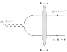
Figure 6: $\gamma\to q\bar{q}$ amplitude in an external shockwave background with the appropriate color representations.

The color structure for this channel is demonstrated in Fig. 6 and it is given by setting $U_{\boldsymbol{b}}^{R_{1}}=U_{\boldsymbol{b}},$ $U_{\boldsymbol{b}}^{R_{2}}=U_{\boldsymbol{b}}^{\dagger}$ and $T^{R_{0}}=1$. This color structure leads to the following TMD operators:

$$\mathcal{O}_{1}^{\left(\gamma\rightarrow q\bar{q}\right)} =-\left(\partial^{j}U_{\boldsymbol{b}}\right)U_{\boldsymbol{b}}^{\dagger}\left(\partial^{j^{\prime}}U_{\boldsymbol{b}^{\prime}}\right)U_{\boldsymbol{b}^{\prime}}^{\dagger}$$

$$\mathcal{O}_{2}^{\left(\gamma\rightarrow q\bar{q}\right)} =\left(\partial^{j}U_{\boldsymbol{b}}\right)U_{\boldsymbol{b}}^{\dagger}\left(\partial^{j^{\prime}}U_{\boldsymbol{b}^{\prime}}\right)U_{\boldsymbol{b}^{\prime}}^{\dagger}$$ (116)

$$\mathcal{O}_{3}^{\left(\gamma\rightarrow q\bar{q}\right)} =\left(\partial^{j}U_{\boldsymbol{b}}\right)U_{\boldsymbol{b}}^{\dagger}\left(\partial^{j^{\prime}}U_{\boldsymbol{b}^{\prime}}\right)U_{\boldsymbol{b}^{\prime}}^{\dagger}$$

$$\mathcal{O}_{4}^{\left(\gamma\rightarrow q\bar{q}\right)} =-\left(\partial^{j}U_{\boldsymbol{b}}\right)U_{\boldsymbol{b}}^{\dagger}\left(\partial^{j^{\prime}}U_{\boldsymbol{b}^{\prime}}\right)U_{\boldsymbol{b}^{\prime}}^{\dagger}.$$

The trace over the color indices can be performed in a straightforward manner and one can easily conclude that this channel involves only one TMD $\mathcal{F}_{gg}^{\left(3\right)}$ which is also referred to as the Weizsäcker-Williams TMD defined in Eq. (64). Using this result and the square of the tensor part given in Eq. (115), we can write the kinematic twist resummed cross section for this channel as

$$\frac{d\sigma_{\gamma\rightarrow q\bar{q}}^{WW}}{dy_{1}dy_{2}d^{2}\boldsymbol{p}_{1}d^{2}\boldsymbol{p}_{2}} =\alpha_{\mathrm{em}}\alpha_{s}p_{0}^{+}\delta\left(p_{1}^{+}+p_{2}^{+}-p_{0}^{+}\right)\frac{z\bar{z}\left(z^{2}+\bar{z}^{2}\right)}{\boldsymbol{p}_{1}^{2}\boldsymbol{p}_{2}^{2}}\mathcal{F}_{gg}^{\left(3\right)}\left(\boldsymbol{k}\right),$$ (117)

which coincides exactly with Eq. (77) by using Eq. (78).

Using the proper color representations for this channel and the dilute limit of the generic CGC cross section given in Eq. (47), we can simply write the dilute limit of the cross section for the $\gamma\to q\bar{q}$ channel as

$$\frac{d\sigma_{\gamma\rightarrow q\bar{q}}^{gA\sim 0}}{dy_{1}dy_{2}d^{2}\boldsymbol{p}_{1}d^{2}\boldsymbol{p}_{2}} =\frac{\alpha_{s}}{16\left(p_{0}^{+}\right)^{2}}\left(2\pi\right)p_{0}^{+}\delta\left(p_{1}^{+}+p_{2}^{+}-p_{0}^{+}\right)\frac{\mathcal{G}\left(\boldsymbol{k}\right)}{\boldsymbol{k}^{2}}\left(\phi^{i}\phi^{j\ast}\right)$$ (118)

$$\times\mathrm{Tr}\left[t^{a}\left(\frac{\boldsymbol{p}_{1}^{i}}{\boldsymbol{p}_{1}^{2}}-\frac{\boldsymbol{q}^{i}}{\boldsymbol{q}^{2}}\right)+t^{a}\left(\frac{\boldsymbol{p}_{2}^{i}}{\boldsymbol{p}_{2}^{2}}+\frac{\boldsymbol{q}^{i}}{\boldsymbol{q}^{2}}\right)\right]\left[t^{c}\left(\frac{\boldsymbol{p}_{1}^{j}}{\boldsymbol{p}_{1}^{2}}-\frac{\boldsymbol{q}^{j}}{\boldsymbol{q}^{2}}\right)+t^{c}\left(\frac{\boldsymbol{p}_{2}^{j}}{\boldsymbol{p}_{2}^{2}}+\frac{\boldsymbol{q}^{j}}{\boldsymbol{q}^{2}}\right)\right],$$

which, after a simple color algebra and using the result for the square of the tensor part given in Eq. (115), leads to

$$\frac{d\sigma_{\gamma\rightarrow q\bar{q}}^{gA\sim 0}}{dy_{1}dy_{2}d^{2}\boldsymbol{p}_{1}d^{2}\boldsymbol{p}_{2}} =\alpha_{\mathrm{em}}\alpha_{s}p_{0}^{+}\delta\left(p_{1}^{+}+p_{2}^{+}-p_{0}^{+}\right)\frac{z\bar{z}\left(z^{2}+\bar{z}^{2}\right)}{\boldsymbol{p}_{1}^{2}\boldsymbol{p}_{2}^{2}}\mathcal{G}\left(\boldsymbol{k}\right).$$ (119)

Finally, we would like to mention that a comparison between Eq. (110) and (112) suggests a similar matching between the iTMD scheme and the dilute limit of the CGC calculation:

$$\sigma_{\gamma\rightarrow q\bar{q}}^{gA\sim 0}=\left.\sigma_{\gamma\rightarrow q\bar{q}}^{WW}\right|_{\mathcal{F}_{gg}^{\left(3\right)}=\mathcal{G}}.$$ (120)

6.5 $q\rightarrow q\gamma$ channel

The last channel we consider is the $q\to q\gamma$ one. The CGC amplitude for this channel is given by Eq. (135) from which we can read off the tensor part as

$$\phi_{\mu}^{\left(q\rightarrow q\gamma\right)} =\frac{-ie_{q}}{2\pi}\varepsilon_{p_{\gamma}\perp}^{\sigma\ast}\bar{u}_{p_{q}}\left[2zg_{\perp\mu\sigma}+\bar{z}\left(\gamma_{\perp\mu}\gamma_{\perp\sigma}\right)\right]\gamma^{+}u_{p}$$ (121)

Its square for an unpolarized observable can be written as

$$\phi^{i\left(q\rightarrow q\gamma\right)}\phi^{i^{\prime}\ast\left(q\rightarrow q\gamma\right)} =\delta^{ii^{\prime}}\left(\frac{e_{q}}{2\pi}\right)^{2}\left(p_{0}^{+}\right)^{2}16z\left(1+z^{2}\right).$$ (122)

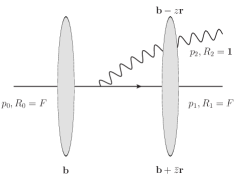
Figure 7: $q\to q\gamma$ amplitude in an external shockwave background with the appropriate color representations.

As it can be seen from Fig. 7, the color structure of this channel is quite simple. One gets the proper color structure by setting $U_{\boldsymbol{b}}^{R_{1}}=U_{\boldsymbol{b}},$ $U_{\boldsymbol{b}}^{R_{2}}=\boldsymbol{1}$ and $T^{R_{0}}=1$. With this simple color structure, only one TMD operator appears in this channel which reads

$$\mathcal{O}^{\left(q\rightarrow q\gamma\right)}=\left(\partial^{j}U_{\boldsymbol{b}}\right)\left(\partial^{j^{\prime}}U_{\boldsymbol{b}^{\prime}}^{\dagger}\right).$$ (123)

Performing the trace over color indices leads to $\mathcal{F}_{qg}^{\left(1\right)}$ TMD which has been introduced in Eq. (60). Plugging these results into Eq. (39), we get the cross section for $q\to q\gamma$ channel:

$$\frac{d\sigma_{q\rightarrow q\gamma}^{WW}}{dy_{1}dy_{2}d^{2}\boldsymbol{p}_{1}d^{2}\boldsymbol{p}_{2}} =\frac{\alpha_{\mathrm{em}}\alpha_{s}}{N_{c}}p_{0}^{+}\delta\left(p_{1}^{+}+p_{2}^{+}-p_{0}^{+}\right)\frac{z\bar{z}^{2}\left(1+z^{2}\right)}{\boldsymbol{p}_{2}^{2}\boldsymbol{q}^{2}}\mathcal{F}_{qg}^{\left(1\right)}\left(\boldsymbol{k}\right),$$ (124)

which coincides exactly with Eq. (79) by using Eq. (80).

Before we continue with the dilute limit for this channel we would like to mention that Eq.(124) is exact and it resums not only the kinematic twists but all twists for this process, i.e. no higher-body twist correction is expected for the $q\to q\gamma$ channel. This is due to the fact that one of the Wilson line operators is trivial for this process and there is no other TMD operator involved.

Inserting the simple color structure of this process into the dilute limit of the generic CGC cross section given in Eq. (47), we get the dilute limit of the cross section for the $q\to q\gamma$ channel:

$$\frac{d\sigma_{q\rightarrow q\gamma}^{gA\sim 0}}{dy_{1}dy_{2}d^{2}\boldsymbol{p}_{1}d^{2}\boldsymbol{p}_{2}} =\frac{\alpha_{s}}{16N_{c}\left(p_{0}^{+}\right)^{2}}\left(2\pi\right)p_{0}^{+}\delta\left(p_{1}^{+}+p_{2}^{+}-p_{0}^{+}\right)\frac{\mathcal{G}_{ac}\left(\boldsymbol{k}\right)}{\boldsymbol{k}^{2}}\left(\phi^{i}\phi^{j\ast}\right)$$ (125)

$$\times\mathrm{Tr}\left[t^{a}\left(\frac{\boldsymbol{p}_{2}^{i}}{\boldsymbol{p}_{2}^{2}}+\frac{\boldsymbol{q}^{i}}{\boldsymbol{q}^{2}}\right)\right]\left[t^{c}\left(\frac{\boldsymbol{p}_{2}^{j}}{\boldsymbol{p}_{2}^{2}}+\frac{\boldsymbol{q}^{j}}{\boldsymbol{q}^{2}}\right)\right],$$

which leads to

$$\frac{d\sigma_{q\rightarrow q\gamma}^{gA\sim 0}}{dy_{1}dy_{2}d^{2}\boldsymbol{p}_{1}d^{2}\boldsymbol{p}_{2}} =\frac{\alpha_{\mathrm{em}}\alpha_{s}}{N_{c}}p_{0}^{+}\delta\left(p_{1}^{+}+p_{2}^{+}-p_{0}^{+}\right)\frac{z\bar{z}^{2}\left(1+z^{2}\right)}{\boldsymbol{p}_{2}^{2}\boldsymbol{q}^{2}}\mathcal{G}\left(\boldsymbol{k}\right).$$ (126)

As in the case of the other channels, comparing Eq. (124) and (126), we also get a straightforward matching between the improved TMD scheme and the dilute scheme:

$$\sigma_{q\rightarrow q\gamma}^{gA\sim 0}=\left.\sigma_{q\rightarrow q\gamma}^{WW}\right|_{\mathcal{F}_{qg}^{\left(1\right)}=\mathcal{G}}.$$ (127)

7 Discussions

Earlier studies have shown that for certain observables the small-$x$ limit of the TMD framework and the so-called ”correlation limit” of the CGC framework overlap. In particular, two particle production (such as dijet or photon+jet) in forward pp and pA collisions, gluon TMDs can be recovered from the CGC calculations in the correlation limit. This specific limit corresponds to the case when the total transverse momentum of the produced particles $\boldsymbol{k}$ is much smaller than the hard scale $Q$. On the other hand, it is also well known that in the dilute limit of the CGC framework, that is in the limit when the total transverse momentum of the produced particles are of the same order as the hard scale, one recovers the BFKL results. Recently, the small-$x$ improved TMD (iTMD) formalism has been developed to interpolate between these two limits.

In this paper we studied two cases. First, by studying the correlation limit of the CGC amplitude for a generic $1\to 2$ process, we identified the kinematic twist contributions from higher order terms in the Taylor expansion of the transverse size of the pair of particles produced in that process, resummed those twist corrections in the Wandzura-Wilczek approximation, i.e. neglecting all genuine twist corrections. The kinematic-twist-resummed cross section for a generic $1\to 2$ process, Eq. (39), is then used to compare the results obtained in the iTMD framework for different channels in forward pp and pA collisions. The perfect matching between these frameworks proves that the iTMD formalism is fully obtained from the CGC formalism by taking the Wandzura-Wilczek approximation.

Second, we considered the dilute limit of the CGC amplitude for a generic $1\to 2$ process. The BFKL amplitudes obtained by taking the dilute limit of the CGC amplitudes are shown to match iTMD results by simply setting the different TMD distributions to the unintegrated parton distribution function that defines the target.

One of the most striking results of this study is the perfect matching between the hard parts of the kinematic twist resummed cross section and the dilute limit of the CGC one. This can be explained in the following way. The kinematic twist resummation procedure that has been developed in this paper isolates and resums the parts of the higher-body contributions which can be rewritten as gauge invariance fixing counterterms to the 1-body hard part. The remaining terms are the genuine twist contributions which vanish in the dilute limit since they account for multiple scatterings. In that sense, we resum the terms which do not vanish in the dilute limit. Thus, the difference between a rigorous twist resummation and the dilute expansion does not lie in the hard parts. Instead, it is linked to the way the hard parts couple to the distributions.

While iTMD distinguishes distributions depending on their gauge link structures, therefore extending its validity range in terms of $\left|\boldsymbol{k}\right|/Q_{s}$ when compared to BFKL, both formalisms rely on the Wandzura-Wilczek approximation in the CGC.

With the previous observations, two origins of saturation can be expected. First of all, the difference between BFKL and iTMD is related to the distinction between gauge link structures, which account for multiple scattering from low $x$ gluons. As discussed earlier, all distributions are equal at large $|\boldsymbol{k}|/Q_{s}$ and distinct at low $|\boldsymbol{k}|/Q_{s}$, were saturation is expected. In that sense, the saturation scale $Q_{s}$ is the parameter which controls the importance of multiple scatterings via gauge links. On the other hand, BFKL and iTMD both rely on the Wandzura-Wilczek approximation when compared to the CGC. It will be very instructive to compare predictions from iTMD and full CGC once genuine twists are extracted from the CGC as well (genuine, ). This would probe $Q_{s}$ as the parameter which controls the importance of multiple scattering via genuine twists.

As a natural extension of this study, we plan to perform a similar analysis for more complex observables where not only the unpolarized TMD distributions but their linearly polarized partners appear. The two immediate observables that we are planning to study are the heavy quark production Marquet:2017xwy and three-particle production such as dijet+photon production Altinoluk:2018byz .

Last but not least, we would like to mention that recently there have been several studies devoted to understand the subeikonal corrections in the CGC framework Altinoluk:2014oxa ; Altinoluk:2015gia ; Altinoluk:2015xuy ; Balitsky:2015qba ; Balitsky:2016dgz ; Balitsky:2017flc ; Chirilli:2018kkw ; Kovchegov:2015pbl ; Kovchegov:2016zex ; Kovchegov:2018znm . Comparing those to the future moderate-$x$ corrections to the iTMD scheme would be also a natural extension of our study.

Appendix A Effective Feynman rules in the external CGC shockwave field

In this appendix, we list the effective Feynman rules that are used to calculate the CGC amplitudes in Appendix B.

Outgoing quark line:

$$\bar{u}\left(p_{q},\,z_{0}\right) = \frac{1}{2}\left(\frac{p_{q}^{+}}{2\pi}\right)^{\frac{d}{2}}\int d^{d}\boldsymbol{x}_{1}e^{ip_{q}^{+}\left(z_{0}^{-}-\frac{\left(\boldsymbol{x}_{1}-\boldsymbol{z}_{0}\right)^{2}}{2z_{0}^{+}}+i0\right)-i\left(\boldsymbol{p}_{q}\cdot\boldsymbol{x}_{1}\right)+i\frac{z_{0}^{+}}{2p_{q}^{+}}\left(m^{2}+i0\right)}\left[U_{\boldsymbol{x}_{1}}\theta\left(-z_{0}^{+}\right)+\theta\left(z_{0}^{+}\right)\right]$$ (128)

$$\times\left(\frac{i}{z_{0}^{+}}\right)^{\frac{d}{2}}\bar{u}_{p_{q}}\gamma^{+}\left(\gamma^{-}-\frac{\hat{x}_{1\perp}-\hat{z}_{0\perp}}{z_{0}^{+}}+\frac{m}{p_{q}^{+}}\right)$$

Outgoing antiquark line:

$$v\left(p_{\bar{q}},\,z_{0}\right) = \frac{1}{2}\left(\frac{p_{\bar{q}}^{+}}{2\pi}\right)^{\frac{d}{2}}\int d^{d}\boldsymbol{x}_{2}e^{ip_{\bar{q}}^{+}\left(z_{0}^{-}-\frac{\left(\boldsymbol{x}_{2}-\boldsymbol{z}_{0}\right)^{2}}{2z_{0}^{+}}+i0\right)-i\left(\boldsymbol{p}_{\bar{q}}\cdot\boldsymbol{x}_{2}\right)+i\frac{z_{0}^{+}}{2p_{\bar{q}}^{+}}\left(m^{2}+i0\right)}\left[U_{\boldsymbol{x}_{2}}^{\dagger}\theta\left(-z_{0}^{+}\right)+\theta\left(z_{0}^{+}\right)\right]$$ (129)

$$\times\left(\frac{i}{z_{0}^{+}}\right)^{\frac{d}{2}}\left(\gamma^{-}-\frac{\hat{x}_{2\perp}-\hat{z}_{0\perp}}{z_{0}^{+}}-\frac{m}{p_{\bar{q}}^{+}}\right)\gamma^{+}v_{p_{\bar{q}}}$$

Incoming gluon line:

$$\varepsilon_{\mu_{0}}^{b_{0}a_{0}}\left(p_{0},\,z_{0}\right) = \left(\frac{p_{0}^{+}}{2\pi}\right)^{\frac{d}{2}}\int d^{d}\boldsymbol{x}_{0}e^{-ip_{0}^{+}\left(z_{0}^{-}-\frac{\left(\boldsymbol{x}_{0}-\boldsymbol{z}_{0}\right)^{2}}{2z_{0}^{+}}-i0\right)+i\left(\boldsymbol{p}_{0}\cdot\boldsymbol{x}_{0}\right)}\left[U_{\boldsymbol{x}_{0}}^{b_{0}a_{0}}\theta\left(z_{0}^{+}\right)+\delta^{a_{0}b_{0}}\theta\left(-z_{0}^{+}\right)\right]$$ (130)

$$\times\left(\frac{-i}{z_{0}^{+}}\right)^{\frac{d}{2}}\left(g_{\perp\mu_{0}\sigma_{0}}+\frac{x_{0\perp\sigma_{0}}-z_{0\perp\sigma_{0}}}{z_{0}^{+}}n_{2\mu_{0}}\right)\varepsilon_{p_{0}\perp}^{\sigma_{0}}$$

Outgoing gluon line:

$$\varepsilon_{\mu}^{ba\ast}\left(p_{g},\,z_{0}\right) = \left(\frac{p_{g}^{+}}{2\pi}\right)^{\frac{d}{2}}\int d^{d}\boldsymbol{x}_{2}e^{ip_{g}^{+}\left(z_{0}^{-}-\frac{\left(\boldsymbol{x}_{2}-\boldsymbol{z}_{0}\right)^{2}-i0}{2z_{0}^{+}}\right)-i\left(\boldsymbol{p}_{g}\cdot\boldsymbol{x}_{2}\right)}\left[U_{\boldsymbol{x}_{2}}^{ab}\theta\left(-z_{0}^{+}\right)+\delta^{ab}\theta\left(z_{0}^{+}\right)\right]$$ (131)

$$\times\left(\frac{i}{z_{0}^{+}}\right)^{\frac{d}{2}}\left(g_{\perp\mu\sigma}+\frac{x_{2\perp\sigma}-z_{0\perp\sigma}}{z_{0}^{+}}n_{2\mu}\right)\varepsilon_{p_{g}\perp}^{\sigma\ast}$$

Appendix B CGC amplitudes for all channels

In this appendix we list the CGC amplitudes calculated by using the effective Feynman rules listed in Appendix A.

$q\rightarrow qg$ channel for forward dijet production in $pp$ and $pA$ collisions:

$$\mathcal{A}_{q\rightarrow qg} =\frac{ig_{s}}{2\pi}\varepsilon_{p_{g}\perp}^{\sigma\ast}\left(2\pi\right)\delta\left(p_{q}^{+}+p_{g}^{+}-p^{+}\right)\int d^{2}\boldsymbol{b}d^{2}\boldsymbol{r}e^{-i\left(\boldsymbol{q}\cdot\boldsymbol{r}\right)-i\left(\boldsymbol{k}\cdot\boldsymbol{b}\right)}$$

$$\times\frac{r_{\perp}^{\mu}}{\boldsymbol{r}^{2}}\left[\left(U_{\boldsymbol{b}+\bar{z}\boldsymbol{r}}t^{b}U_{\boldsymbol{b}-z\boldsymbol{r}}^{ab}\right)-\left(t^{b}\delta^{ab}U_{\boldsymbol{b}}\right)\right]$$ (132)

$$\times\bar{u}_{p_{q}}\left[2zg_{\perp\mu\sigma}+\bar{z}\left(\gamma_{\perp\mu}\gamma_{\perp\sigma}\right)\right]\gamma^{+}u_{p}$$

$g\rightarrow q\bar{q}$ channel for forward dijet production in $pp$ and $pA$ collisions:

$$\mathcal{A}_{g\rightarrow q\bar{q}} =-i\frac{g_{s}}{2\pi}\varepsilon_{p\perp}^{\sigma}\left(2\pi\right)\delta\left(p_{q}^{+}+p_{\bar{q}}^{+}-p_{g}^{+}\right)\int d^{2}\boldsymbol{b}d^{2}\boldsymbol{r}e^{-i\left(\boldsymbol{q}\cdot\boldsymbol{r}\right)-i\left(\boldsymbol{k}\cdot\boldsymbol{b}\right)}$$

$$\times\frac{r_{\perp}^{\mu}}{\boldsymbol{r}^{2}}\left[\left(U_{\boldsymbol{b}+\bar{z}\boldsymbol{r}}t^{b}U_{\boldsymbol{b}-z\boldsymbol{r}}^{\dagger}\delta^{ab}\right)-\left(t^{b}U_{\boldsymbol{b}}^{ba}\right)\right]$$ (133)

$$\times\bar{u}_{p_{q}}\left[2zg_{\perp\mu\sigma}-\left(\gamma_{\perp\mu}\gamma_{\perp\sigma}\right)\right]\gamma^{+}v_{p_{\bar{q}}}$$

$g\rightarrow gg$ channel for forward dijet production in $pp$ and $pA$ collisions:

$$\mathcal{A}_{g\rightarrow gg} =\frac{2g_{s}p^{+}}{\pi}\varepsilon_{p\perp}^{\sigma_{0}}\varepsilon_{p_{g}\perp}^{\sigma_{1}\ast}\varepsilon_{q_{g}\perp}^{\sigma_{2}\ast}\left(2\pi\right)\delta\left(p_{g}^{+}+q_{g}^{+}-p^{+}\right)\int d^{2}\boldsymbol{b}d^{2}\boldsymbol{r}e^{-i\left(\boldsymbol{q}\cdot\boldsymbol{r}\right)-i\left(\boldsymbol{k}\cdot\boldsymbol{b}\right)}$$

$$\times\frac{r_{\perp}^{\mu}}{\boldsymbol{r}^{2}}\left[f^{b_{0}b_{1}b_{2}}\delta^{b_{0}a_{0}}U_{\boldsymbol{b}+\bar{z}\boldsymbol{r}}^{b_{1}a_{1}}U_{\boldsymbol{b}-z\boldsymbol{r}}^{b_{2}a_{2}}-f^{b_{0}b_{1}b_{2}}\delta^{b_{1}a_{1}}\delta^{b_{2}a_{2}}U_{\boldsymbol{b}}^{b_{0}a_{0}}\right]$$ (134)

$$\times\left[zg_{\perp\sigma_{0}\sigma_{1}}g_{\perp\mu\sigma_{2}}-z\bar{z}g_{\perp\sigma_{1}\sigma_{2}}g_{\perp\mu\sigma_{0}}+\bar{z}g_{\perp\sigma_{0}\sigma_{2}}g_{\perp\mu\sigma_{1}}\right]$$

Production of a forward photon-jet pair in $pp$ and $pA$ collisions:

$$\mathcal{A}_{q\rightarrow q\gamma} =\frac{ig_{s}}{2\pi}\varepsilon_{p_{\gamma}\perp}^{\sigma\ast}\left(2\pi\right)\delta\left(p_{q}^{+}+p_{g}^{+}-p^{+}\right)\int d^{2}\boldsymbol{b}d^{2}\boldsymbol{r}e^{-i\left(\boldsymbol{q}\cdot\boldsymbol{r}\right)-i\left(\boldsymbol{k}\cdot\boldsymbol{b}\right)}$$

$$\times\frac{r_{\perp}^{\mu}}{\boldsymbol{r}^{2}}\left(U_{\boldsymbol{b}+\bar{z}\boldsymbol{r}}-U_{\boldsymbol{b}}\right)\bar{u}_{p_{q}}\left[2zg_{\perp\mu\sigma}+\bar{z}\left(\gamma_{\perp\mu}\gamma_{\perp\sigma}\right)\right]\gamma^{+}u_{p}$$ (135)

Appendix C The integral

In this appendix, we present the details of the calculation of the following integral

$$I^{ij}\left(\boldsymbol{p}\right) \equiv\int d^{d}\boldsymbol{r}\frac{\boldsymbol{r}^{i}\boldsymbol{r}^{j}}{\boldsymbol{r}^{2}}\frac{e^{-i\left(\boldsymbol{p}\cdot\boldsymbol{r}\right)}-1}{\left(\boldsymbol{p}\cdot\boldsymbol{r}\right)}e^{-i\left(\boldsymbol{q}\cdot\boldsymbol{r}\right)}.$$ (136)

This integral is a symmetric tensor, hence we can decompose it in a 3-dimensional basis. Let us choose

$$\left(\delta^{ij},\frac{\boldsymbol{p}^{i}\boldsymbol{q}^{j}+\boldsymbol{q}^{j}\boldsymbol{p}^{i}}{\boldsymbol{p}\cdot\boldsymbol{q}},\frac{\boldsymbol{p}^{i}\boldsymbol{p}^{j}}{\boldsymbol{p}^{2}}\right),$$ (137)

and write

$$I^{ij}\left(\boldsymbol{p}\right)=I_{0}\delta^{ij}+I_{1}\frac{\boldsymbol{p}^{i}\boldsymbol{q}^{j}+\boldsymbol{q}^{i}\boldsymbol{p}^{j}}{\boldsymbol{p}\cdot\boldsymbol{q}}+I_{2}\frac{\boldsymbol{p}^{i}\boldsymbol{p}^{j}}{\boldsymbol{p}^{2}}.$$ (138)

This relations inverts to

$$I_{0} =I^{ii}\left(\boldsymbol{p}\right)-\frac{\boldsymbol{p}^{i}\boldsymbol{p}^{j}}{\boldsymbol{p}^{2}}I^{ij}\left(\boldsymbol{p}\right)$$

$$I_{1} =-\frac{\left(\boldsymbol{p}\cdot\boldsymbol{q}\right)^{2}}{\boldsymbol{p}^{2}\boldsymbol{q}^{2}-\left(\boldsymbol{p}\cdot\boldsymbol{q}\right)^{2}}\frac{\boldsymbol{p}^{i}\boldsymbol{p}^{j}}{\boldsymbol{p}^{2}}I^{ij}\left(\boldsymbol{p}\right)+\frac{\left(\boldsymbol{p}\cdot\boldsymbol{q}\right)}{\boldsymbol{p}^{2}\boldsymbol{q}^{2}-\left(\boldsymbol{p}\cdot\boldsymbol{q}\right)^{2}}\boldsymbol{p}^{i}\boldsymbol{q}^{j}I^{ij}\left(\boldsymbol{p}\right)$$ (139)

$$I_{2} =-I^{ii}\left(\boldsymbol{p}\right)+\frac{2\boldsymbol{p}^{2}\boldsymbol{q}^{2}}{\boldsymbol{\boldsymbol{p}}^{2}\boldsymbol{q}^{2}-\left(\boldsymbol{p}\cdot\boldsymbol{q}\right)^{2}}\frac{\boldsymbol{p}^{i}\boldsymbol{p}^{j}}{\boldsymbol{p}^{2}}I^{ij}\left(\boldsymbol{p}\right)-\frac{2\left(\boldsymbol{p}\cdot\boldsymbol{q}\right)}{\boldsymbol{p}^{2}\boldsymbol{q}^{2}-\left(\boldsymbol{p}\cdot\boldsymbol{q}\right)^{2}}\boldsymbol{p}^{i}\boldsymbol{q}^{j}I^{ij}\left(\boldsymbol{p}\right).$$

Thus in order to compute $I^{ij}$, it is sufficient to compute $J_{0}=\delta^{ij}I^{ij}$ and $J_{1}^{j}\equiv\boldsymbol{\boldsymbol{p}}^{i}I^{ij}.$ One can actually show that $J_{0}=0$. This becomes apparent by going to spherical coordinates, integrating $\left|\boldsymbol{r}\right|$ out (taking into account the phase regulators $i0$ in the exponent from the effective rules in Appendix A) and checking that the remaining angular integral is null.

$J_{1}^{j}$ is obtained easily with the usual Schwinger representation tricks and reads:

$$J_{1}^{j}=-2i\pi\left(\frac{\boldsymbol{q}^{j}+\boldsymbol{\boldsymbol{p}}^{j}}{\left(\boldsymbol{q}+\boldsymbol{p}\right)^{2}}-\frac{\boldsymbol{q}^{j}}{\boldsymbol{q}^{2}}\right).$$ (140)

Finally plugging Eq. (140) in Eq. (139) then in Eq. (138), one obtains

$$I^{ij}\left(\boldsymbol{k}\right)=-2\frac{i\pi}{\boldsymbol{p}^{2}}\left[\left(\frac{\left(\boldsymbol{p}\cdot\boldsymbol{q}\right)}{\boldsymbol{q}^{2}}-\frac{\left(\boldsymbol{p}\cdot\boldsymbol{q}\right)+\boldsymbol{\boldsymbol{p}}^{2}}{\left(\boldsymbol{q}+\boldsymbol{p}\right)^{2}}\right)\delta^{ij}+\left(\frac{1}{\left(\boldsymbol{q}+\boldsymbol{p}\right)^{2}}-\frac{1}{\boldsymbol{q}^{2}}\right)\left(\boldsymbol{p}^{i}\boldsymbol{q}^{j}+\boldsymbol{q}^{i}\boldsymbol{p}^{j}\right)+2\frac{\boldsymbol{p}^{i}\boldsymbol{p}^{j}}{\left(\boldsymbol{q}+\boldsymbol{p}\right)^{2}}\right],$$ (141)

which leads to the expression given in Eq. (37).