Heat Bath Algorithmic Cooled Quantum Otto Engines

Abstract

We suggest alternative quantum Otto engines, using heat bath algorithmic cooling with partner pairing algorithm instead of isochoric cooling. Liquid state nuclear magnetic resonance systems in one entropy sink are considered as working fluids. Then, the extractable work and thermal efficiency are analyzed in detail for four-stroke and two-stroke type of quantum Otto engines. The role of heat bath algorithmic cooling in these cycles is to use a single entropy sink instead of two. Also, this cooling algorithm increases the power of engines reducing the time required for one cycle.

I Introduction

With the advances of miniaturized information and energy devices, the question of whether using a quantum system to harvest a classical resource can have an advantage over a classical harvester has gained much attention in recent years Quan et al. (2007); Huang et al. (2014); Thomas and Johal (2014); Zhang et al. (2007); Huang et al. (2013); Thomas and Johal (2011); Scully et al. (2003); Zhang (2008); Thomas and Johal (2011); Çakmak et al. (2016); Zhang et al. (2014); Türkpençe and Müstecaplıoğlu (2016); Chand and Biswas (2017a, b); Quan et al. (2007); Uzdin et al. (2015); Alecce et al. (2015); Scovil and Schulz-DuBois (1959); Alicki (1979); Linden et al. (2010); Uzdin and Kosloff (2014); Gelbwaser-Klimovsky et al. (2013); Kosloff and Levy (2014); Feldmann and Kosloff (2003); Roßnagel et al. (2016); Abah et al. (2012). The argument is more or less settled in the case of quantum information devices, and the main challenge remained is their efficient implementation. In typical quantum information devices, both the inputs and the algorithmic steps of operation are of completely quantum nature. In contrast, quantum energy devices process incoherent inputs and they operate with thermodynamical processes being quantum analogs of their classical counterparts. The quantum superiority in such a thermal device reveals itself when the resource has some quantum character, for example squeezing Klaers et al. (2017); Roßnagel et al. (2014), or when the harvester has profound quantum nature, for example, quantum correlations Dillenschneider and Lutz (2009); Dağ et al. (2016). Studies of both cases are limited to machine processes analogs of classical thermodynamical ones. Here we ask how can we use genuine quantum steps in the machine operation and if we can do so what are the quantum advantages we can get.

As a specific system to explore completely quantum steps in thermal quantum device operation we consider an NMR system. Very recently NMR quantum heat engines become experimentally available Peterson et al. (2018); De Assis et al. (2018). Power outputs of these machines are not optimized. One can use non-classical resources, though such a resource would not be natural and require some generation cost reducing overall efficiency. Alternatively one can use dynamical shortcuts to speeding up adiabatic transformations Çakmak et al. (2017) but this would increase experimental complexity, and moreover in NMR thermalization is more seriously slow step reducing the power output of the NMR machines.

Here we, propose to replace adiabatic steps by SWAP operations while the cooling step by an algorithmic cooling Park et al. (2016); Rodríguez-Briones and Laflamme (2016); Atia et al. (2016); Brassard et al. (2014a, b); Fernandez et al. (2004); Elias et al. (2007); Boykin et al. (2002); Kafri and Taylor (2012); Raeisi and Mosca (2015); Rodríguez-Briones et al. (2017); Ryan et al. (2008); Schulman et al. (2005); Elias et al. (2006). By this way, NMR thermal device operation would closely resemble an NMR quantum computer Oliveira et al. (2007); Devoret et al. (2011); Abragam (1963); Goold et al. (2016) albeit processing a completely noisy input. We remark that there will be only the classical energy source as the input to the machine, while the second heat bath required by the second law of thermodynamics for work production would be an effective one, engineered by a spin ensemble, typical in the algorithmic cooling scheme. In addition to engine cycles, NMR systems were also proposed for studies of single-shot thermodynamics Batalhão et al. (2014).

Our scheme allows us to provide at least one answer, in the context of NMR heat engines, to the question of how to implement genuine quantum steps in quantum machine operation to harvest a classical energy source. In addition, our calculations suggest that compared to the NMR engine with standard thermodynamical steps quantum algorithmic NMR engine produce more power. The advantage comes from the replacing the long-time isochoric cooling process with the more efficient and fast algorithmic cooling stage. We provide systematic investigation by first examining the case of standard Otto cycle as a benchmark then introduce the algorithmic cooling stage instead of isochoric cooling one, and finally introduce the SWAP operation stages instead of the adiabatic transformations.

The organization of the paper is as follows. We review the theory and heat bath algorithmic cooling (HBAC) considering 3-qubit NMR sample in Sec. II. The results and discussions are given in Sec. III. In Sec. III.1, efficiency, work, and power output of four-stroke quantum Otto cycles cooled by HBAC and isochoric stage are discussed by considering the same parameters to extract work. Two-stroke type engine results are discussed in Sec. III.2. We conclude in Sec. IV. The details of the HBAC using partner pairing algorithm (PPA) are given in Appendix A.

II THE WORKING FLUID

Quantum Otto engines (QOEs) consist of quantum adiabatic and isochoric processes Çakmak et al. (2017). Three types of quantum Otto cycle is given in the literature as four-stroke, two-stroke, and continuous Quan et al. (2007); Uzdin et al. (2015). In this article, four-stroke, and two-stroke type of QOEs are examined. The basic model of HBAC with PPA is considered instead of isochoric cooling. Implementation of HBAC requires two sets of qubits; reset qubits and computational qubits. One of the computational qubits operated as target qubit which is going to be cooled by applying PPA while other computational qubits play a role in entropy compression Rodríguez-Briones and Laflamme (2016). This cooling process can be implemented with a minimal system composed of just 3-qubit Atia et al. (2016); Brassard et al. (2014a); Park et al. (2016); Rodríguez-Briones and Laflamme (2016). For the four-stroke engine, we consider the target qubit as the working fluid (see Fig. 1).

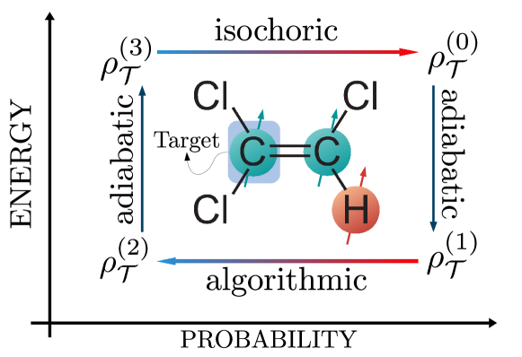
Figure 1: (Color online) Four-stroke quantum heat engine operating in a single heat bath at temperature $T$. It has one isochoric heating process, two adiabatic processes and one algorithmic cooling process.

As the working substance for two-stroke QOEs, we again chose the target qubit of the 3-qubit system, but with an extra qubit coupled to the target qubit (see Fig. 2).

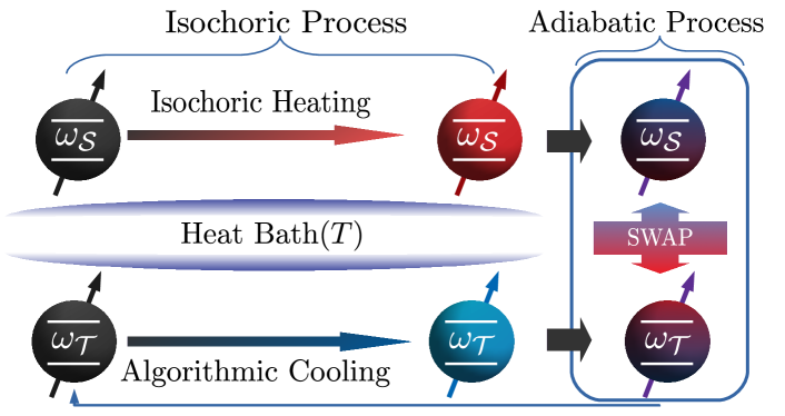
Figure 2: (Color online) Two-stroke quantum heat engine operating in a single heat bath at temperature $T$. It has isochoric heating process and algorithmic cooling process happen at the same time. Then, one adiabatic process using SWAP operation.

In NMR systems, various 3-qubit models have been used for quantum information processing Hou et al. (2014); Li et al. (2011); Henry et al. (2006); Cummins et al. (2002). To make an applicable and realistic model for QOEs using these systems, a suitable sample and a well-designed procedure must be considered. We used parameters of ${}^{13}\mathrm{C_{2}}$-trichloroethylene (TCE) (see Table 1) with paramagnetic reagent $\mathrm{Cr(acac)_{3}}$ in cloroform-d solution ($\mathrm{CDCl_{3}}$) in our numerical calculations, which are also experimentally used for HBAC in Refs. Atia et al. (2016); Brassard et al. (2014a). Carbon-1 and Carbon-2 qubits are classified as the target and the compression qubits. And, Hydrogen qubit is selected as the reset qubit because of the relaxation time, which is small compared to the other two qubits. To implement HBAC, the Hamiltonian of 3-qubit in the lab frame can be written as Oliveira et al. (2007)

$$H^{(0)}=-\hbar\sum_{i}\omega_{i}I_{iz}+\hbar\sum_{i\neq j}J_{ij}I_{iz}I_{jz},\quad i,j=\{\mathcal{T},\mathcal{C},\mathcal{R}\},$$ (1)

where, $\omega_{i}=\gamma_{i}B_{z}$ is the characteristic frequency of the $i^{th}$ qubit, $\gamma_{i}$ is the nuclear gyromagnetic ratio and $B_{z}$ is the magnetic field. $\mathcal{T}$, $\mathcal{C}$ and $\mathcal{R}$ stand for target, compression and reset qubits, respectively. $I_{z}$ is the component of the spin angular momentum of the $i^{th}$ qubit and $J_{ij}$ is the scalar isotropic coupling strength between $i^{th}$ and $j^{th}$ qubits.

	Target-C1	Compression-C2	Reset-H
$\gamma/2\pi$	10.7084 [MHz/T]	10.7084 [MHz/T]	42.477 [MHz/T]
$\omega/2\pi$	125.77 [MHz]	125.77 [MHz]	500.13 [MHz]
$\tau^{1}$	43 [s]	20 [s]	3.5 [s]
	C1-C2	C1-H	C2-H
$J/2\pi$	103 [Hz]	9 [Hz]	200.8 [Hz]

Table 1: The first row in the table shows gyromagnetic ratio values of Carbon1, Carbon2 and Hydrogen qubits. Considering the 500Mhz NMR device, the corresponding characteristic frequencies are given in the second row. Also, their experimental $\tau^{1}$ relaxiation times are given in the third row. Last row shows J-coupling strenght between these qubits Atia et al. (2016); Brassard et al. (2014a).

III RESULTS AND DISCUSSION

III.1 Four-stroke Heat Bath Algoritmic Cooled Quantum Otto Engine

Normally, four-stroke QOEs consist of two isochoric and two adiabatic stages. However, we consider one isochoric stage, one algorithmic cooling stage, and two adiabatic stages (see Fig. 1). The details of the four stroke cycle is described as follows.

Isochoric Heating: 3-qubit of TCE molecule with Hamiltonian in Eq. (1) is in contact with a heat bath at temperature T=300 K. The density matrix of the 3-qubit system at the end of this stage is given by

$$\rho_{\mathrm{th}}^{(0)}=\frac{e^{-\beta H^{(0)}}}{Z}.$$ (2)

Here $Z=\mathrm{Tr}\left[e^{-\beta H^{(0)}}\right]$ is the partition function and $\beta=1/k_{B}T$. The initial density matrix of our working fluid can be expressed by taking a partial trace of 3-qubit system

$$\rho_{\mathcal{T}}^{(0)}=\mathrm{Tr}_{{\mathcal{C,R}}}\left[\rho_{\mathrm{th}}^{(0)}\right].$$ (3)

Adiabatic Compression: Qubits are isolated from the heat bath and undergo finite-time adiabatic expansion. The adiabatic processes of the cycle are assumed to be generated by a time-dependent magnetic field Kosloff (2013); Vinjanampathy and Anders (2016). Here, $H^{(0)}$ at $t=0$ is changed to $H^{(1)}$ at $t=\tau/2$ by driving the initial magnetic field as $B_{z}\rightarrow B_{z}/2$. The time evolution of the density matrix is governed by the Liouville-von Neumann equation $\dot{\rho}(t)=-[H(t),\rho(t)]$, and $H(t)$ can be expressed as $H(t)=H^{(0)}+H_{\mathrm{drive}}$, where $H_{\mathrm{drive}}$ is given by

$$H_{\mathrm{{drive}}}=\hbar\sum_{i}\left(\omega_{i}-\omega_{i}^{\prime}\right)I_{iz}\sin\left(\frac{\pi t}{\tau}\right).$$ (4)

Here, $\omega_{i}^{\prime}=\gamma_{i}B_{z}/2$ is the characteristic frequency at the end of the adiabatic stage. Up to this point, we used Hamiltonian in Eq (1) which is written for 3-qubit. However, to find the work done in this stage, we need to consider only the target qubit. The local Hamiltonian for target qubit before adiabatic compression can be written as $H^{(0)}_{\mathcal{T}}=-\hbar\omega_{\mathcal{T}}I_{z}$. After the adiabatic compression, it will be $H^{(1)}_{\mathcal{T}}=-\hbar\omega_{\mathcal{T}}^{\prime}I_{z}$. The initial density matrix of the target qubit $(t=0)$ is given in Eq (3). The final density matrix of 3-qubit system at the end of adiabatic compression is $\rho^{(1)}=\rho(\tau/2)$. The density matrix of the target qubit at the end of this process is $\rho_{\mathcal{T}}^{(1)}=\mathrm{Tr}_{{\mathcal{C,R}}}\left[\rho^{(1)}\right]$. Then, the work performed by the working fluid is

$$W_{1}=\mathrm{Tr}\left[H^{(0)}_{\mathcal{T}}\rho_{\mathcal{T}}^{(0)}\right]-\mathrm{Tr}\left[H^{(1)}_{\mathcal{T}}\rho_{\mathcal{T}}^{(1)}\right].$$ (5)

Heat Bath Algorithmic Cooling: In this part of the engine, we normally need a cold heat bath to cool down our target qubit. Instead of using a cold heat bath, the working fluid treated in the same heat bath as isochoric heating. Thus, to cool down the target qubit HBAC is used. Details of the cooling mechanism given in the Appendix A. For each qubit, polarization is defined as

$$\epsilon_{i}=P^{\uparrow}_{i}-P^{\downarrow}_{i}=\tanh\left(\frac{\hbar\gamma_{i}B_{z}}{2k_{B}T}\right),$$ (6)

where, $P^{\uparrow}_{i}$ and $P^{\downarrow}_{i}$ denote the probability of up and down states. In a closed quantum system, Shannon’s bound limits the polarization of single spin in a collection of equilibrium spin system. Using HBAC take advantage of the heat bath to cool the target qubit beyond Shannon’s bound Atia et al. (2016). As a result, the polarization of the target qubit using HBAC becomes higher than the polarization of the heat bath.

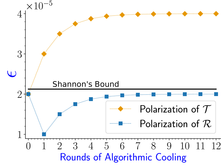
Figure 3: (Color online) The polarization $\epsilon$ (dimensionless) calculated by using the Eq. (7) for each rounds of algorithmic cooling. The target and reset qubits polarizations calculated by taking into account the perfectly applied quantum logic gates in terms of several rounds of the PPA. The black line shows Shannon’s limit of polarization. The polarization of the target qubit has exceeded this limit after the first iteration and the reset qubit stays under this limit.

After the first SWAP operation before PPA, polarizations of the qubits are equal to each other. The value of their polarization is given at zeroth iteration in Fig. 3 as $\sim 2.0\times 10^{-5}$. Then, several rounds of PPA are applied. The effective temperature of the target qubit is determined by Eq. (7) and plotted in Fig. 4. The target qubit reached a polarization above the Shannon limit as a result of one round of PPA and target qubit cooled down to $\sim 50\mathrm{K}$. After seven rounds of PPA, it almost reached to its maximum value as $\sim 4.0\times 10^{-5}$ and cool down to $\sim 37\mathrm{K}$ temperature. At the end of PPA, density matrix of target qubit is given by Eq. (22) as

$$\rho^{(2)}_{\mathcal{T}}=\mathrm{Tr}_{\mathcal{C,R}}\left[\rho^{(1,5)}_{AC}\right].$$ (7)

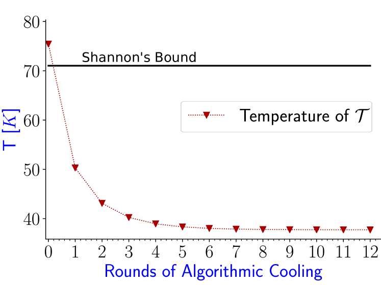
Figure 4: (Color online) The effective temperature of target qubit calculated by using the relation between temperature and polarization given in Eq. 7. The black line shows the corresponding Shannon’s limit of temperature. The effective temperature of the target qubit has exceeded this limit after the first iteration.

Adiabatic Expansion: In this process $H^{(1)}$ at $t=0$ is changed to $H^{(0)}$ at $t=\tau/2$ by driving back the magnetic field as $B_{z}/2\rightarrow B_{z}$. The work performed by the target qubit in this process can be written as

$$W_{2}=\mathrm{Tr}\left[H^{(1)}_{\mathcal{T}}\rho^{(2)}_{\mathcal{T}}\right]-\mathrm{Tr}\left[H^{(0)}_{\mathcal{T}}\rho^{(3)}_{\mathcal{T}}\right].$$ (8)

Work and Power Output of Four-Stroke QOE: The total work done by the working fluid at the end of adiabatic stages can be found as $W=W_{1}+W_{2}$. Alternatively, total work can also be calculated from the isochoric stage and algorithmic cooling stage using $W=Q_{\text{in}}-Q_{\text{out}}$ where, $Q_{\text{in}}=\mathrm{Tr}\left[H^{(0)}_{\mathcal{T}}(\rho^{(3)}_{\mathcal{T}}-\rho^{(0)}_{\mathcal{T}})\right]$ and $Q_{\text{out}}=\mathrm{Tr}\left[H^{(1)}_{\mathcal{T}}(\rho^{(2)}_{\mathcal{T}}-\rho^{(1)}_{\mathcal{T}})\right]$ are the heat released and absorbed in these stages, respectively. The efficiency of the cycle is determined by $\eta=1-\omega_{\mathcal{T}}^{\prime}/\omega_{\mathcal{T}}$ and for this engine $\eta=0.5$. In Fig. 5 , we plot the heat released and absorbed by the target qubit as per rounds of PPA. As the number of iterations increases, it can be observed that the absorbed heat increases more than the heat released. After the first iteration, the target qubit absorbed $\sim 5\times 10^{-7}\mathrm{J/mol}$ of heat and released $\sim 2.5\times 10^{-7}\mathrm{J/mol}$ of heat. As a result $\sim 2.5\times 10^{-7}\mathrm{J/mol}$ work was performed.

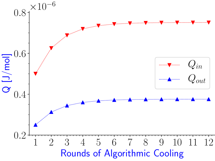
Figure 5: (Color online) Heat absorbed and released in a four-stroke cycle by the target qubit in the isochoric process ($Q_{in}$) and algorithmic cooling process ($Q_{out}$) for per rounds of PPA.

In order to see the difference in power caused by the algorithmic cooling and isochoric processes, we consider cold baths, corresponding to the temperatures in Fig. 4, to simulate a quantum Otto cycle cooled by isochoric stage with same parameters. By this way, the work output of the quantum Otto cycle cooled by isochoric stage will be the same as the cycle cooled by HBAC (see Fig 6). As we can see from Fig. 6; while the work produced by the target qubit rapidly increases with the number of iterations at the beginning, it remains constant after a certain iteration of the PPA. The reason for this behavior, the HBAC is able to cool the target qubit up to a certain limit. In Fig. 5 , after the fourth iteration, the target qubit almost reaches the maximum value it can absorb and release heat. Absorbed and released heat from qubit in the cycle at this iteration is $\sim 3.5\times 10^{-7}\mathrm{J/mol}$ and $\sim 7.2\times 10^{-7}\mathrm{J/mol}$. Then, maximum work output of the cycle is $\sim 3.7\times 10^{-7}\mathrm{J/mol}$ (see Fig. 6).

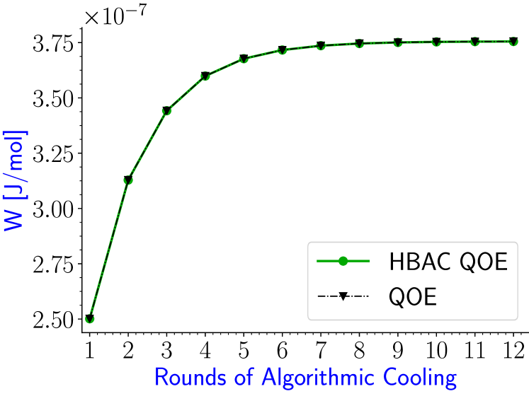
Figure 6: (Color online) Work obtained, in a four-stroke cycle per number of iteration of PPA, from target qubits of one mol of TCE cooled by HBAC (green line). And work obtained from a mol of qubits, which are cooled by isochoric stage to temperatures corresponding in Fig 4 (black line).

The number of iteration of PPA is important for quantum heat engines. Because more iteration means that more relaxation of reset qubit and it increases the time required to complete engine cycle. Even if we increase the work output iterating more PPA, we may lose power output. For a quantum Otto cycle using NMR system as working fluid, the adiabatic stages of the cycle are considered as fast compared to the isochoric stages Çakmak et al. (2017). We estimate the power output of cycles considering isochoric stages and HBAC. A single number of iteration of PPA requires two reset process. Taking the number of iteration ’n’, we can write power output for quantum Otto cycle using HBAC as $P={W}/{(\tau_{\mathcal{T}}+\tau_{\mathcal{R}}(2n+1))},$ where, $\tau_{\mathcal{T}}$ and $\tau_{\mathcal{R}}$ are relaxation times of the Carbon1 and the Hydrogen qubits respectively from the Table  1. For the cycle using isochoric process in the cooling stage, power output is $P=W/2\tau_{\mathcal{T}}$. In Fig. 7, we plot power output for these engines. We see that the second iteration of PPA gives maximum power output as $\sim 5.2\times 10^{-9}$ Watt/mol. For more number of iteration, this power output is getting decrease.

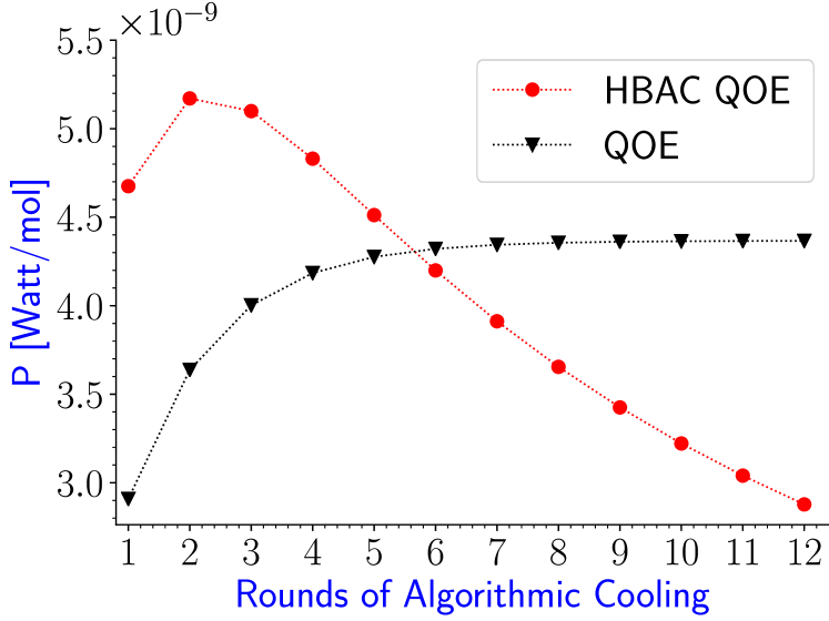
Figure 7: (Color online) Power output for a four-stroke cycle per number of iteration of PPA, from target qubit of one mol TCE, cooled by HBAC (red) and from a mol of qubits cooled by isochoric stage to temperatures corresponding in Fig 4 (black).

After the fifth iteration of PPA, the cycle using the isochoric cooling stage can dominate the engine using the HBAC stage. Accordingly, the optimum choice of the number of rounds in HBAC is two for our four-stroke model system. Such a choice optimizes the power output of the cycle yielding high power performance.

III.2 Two-Stroke Heat-Bath Algorithmic Cooled Quantum Otto Engine

We also investigate two-stroke QOE that is proposed in Refs. Quan et al. (2007); Uzdin et al. (2015). To construct it, we need to consider two qubits donated as $\mathcal{S}$ and $\mathcal{T}$ as the working fluid. First, two qubits are isolated from each other. One of the qubits contacts with a heat bath at temperature T until it reaches to equilibrium. Our purpose is to cool the other qubit within the same heat bath utilizing algorithmic cooling. Hence we need another two qubits for this process as compression qubit and reset qubit. This part is considered as two isochoric processes for the heat engine. Second, two qubits decouple from the heat bath. Then, the SWAP operation is performed between these two qubits (see Fig. 8).

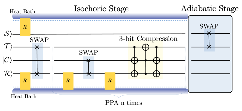
Figure 8: Quantum circuit demonstrating the two stroke heat bath algorithmic cooled quantum Otto engine. $|\mathcal{S}\rangle$ stands for qubit $\mathcal{S}$ and $|\mathcal{T}\rangle$ for qubit $\mathcal{T}$. Here, isochoric heating demonstrated as R operation and applied only one time on qubit $\mathcal{S}$. For qubit $\mathcal{T}$, PPA applied and it is given in Appendix A. After these two process finished SWAP operation applied between two qubits and cycle is completed with adiabatic process.

Local Hamiltonian of the qubit $\mathcal{S}$ and qubit $\mathcal{T}$ can be written as $H_{\mathcal{S}}=-\hbar\omega_{\mathcal{S}}I_{z}$ and $H_{\mathcal{T}}=-\hbar\omega_{\mathcal{T}}I_{z}$, respectively. And density matrix of qubit $\mathcal{S}$, at the end of the isochoric stage is given by $\rho^{(0)}_{\mathcal{S}}=e^{-\beta H_{\mathcal{S}}}/{Z}$. Using the PPA given in the Appendix A, we can write the density matrix of qubit $\mathcal{T}$ at the end of HBAC as $\rho^{(0)}_{\mathcal{T}}=\mathrm{Tr}_{\mathcal{C,R}}\left[\rho^{(1,5)}_{AC}\right]$. It is assumed that the coupling between $\mathcal{S}$ and $\mathcal{T}$ qubits are small compered to $\omega_{\mathcal{S}}$ and $\omega_{\mathcal{T}}$. The density matrix of the total working fluid can be expressed as

$$\rho_{\mathcal{S,T}}^{(0)}\approx\rho^{(0)}_{\mathcal{S}}\otimes\rho^{(0)}_{\mathcal{T}}.$$ (9)

In the adiabatic process, a SWAP gate is applied to exchange the states of $\mathcal{S}$ and $\mathcal{T}$ qubits

$$\rho_{\mathcal{S,T}}^{(1)}=\mathrm{SWAP}\left(\rho_{\mathcal{S,T}}^{(0)}\right)\mathrm{SWAP}^{\dagger}.$$ (10)

At the end of the cycle, density matrices of individual qubits become

$$\rho^{(1)}_{\mathcal{S}}=\mathrm{Tr}_{\mathcal{T}}\left[\rho^{(1)}_{\mathcal{S,T}}\right],\quad\rho^{(1)}_{\mathcal{T}}=\mathrm{Tr}_{\mathcal{S}}\left[\rho^{(1)}_{\mathcal{S,T}}\right].$$ (11)

Heat absorbed by the qubit $\mathcal{S}$ calculated as follows

$$Q_{in}=\mathrm{Tr}\left[H_{\mathcal{S}}\rho^{(0)}_{\mathcal{S}}\right]-\mathrm{Tr}\left[H_{\mathcal{S}}\rho^{(1)}_{\mathcal{S}}\right],$$ (12)

and the heat released by the qubit $\mathcal{T}$ is

$$Q_{out}=\mathrm{Tr}\left[H_{\mathcal{T}}\rho^{(1)}_{\mathcal{T}}\right]-\mathrm{Tr}\left[H_{\mathcal{T}}\rho^{(0)}_{\mathcal{T}}\right].$$ (13)

The net work is evaluated by $W=Q_{\mathrm{in}}-Q_{\mathrm{out}}$, with efficiency $\eta=1-\omega_{\mathcal{T}}/\omega_{\mathcal{S}}$. To get a positive work, the frequency of qubit $\mathcal{S}$ needs to be greater than the frequency of the qubit $\mathcal{T}$ ($\omega_{\mathcal{S}}>\omega_{\mathcal{T}}$). In addition, $T>T_{\mathcal{T}}({\omega_{\mathcal{S}}}/{\omega_{\mathcal{T}}})$ needs to be satisfied. Here $T_{\mathcal{T}}$ is the temperature of target qubit in HBAC. Positive work conditions then can be expressed as

$$\omega_{\mathcal{T}}<\omega_{\mathcal{S}}<\omega_{\mathcal{T}}\frac{T}{T_{\mathcal{T}}}.$$ (14)

Fig. 9 shows the relation between the work output and $\omega_{\mathcal{S}}$, for different number of iterations. When the number of iteration of PPA is increased, the best work output is also increased.

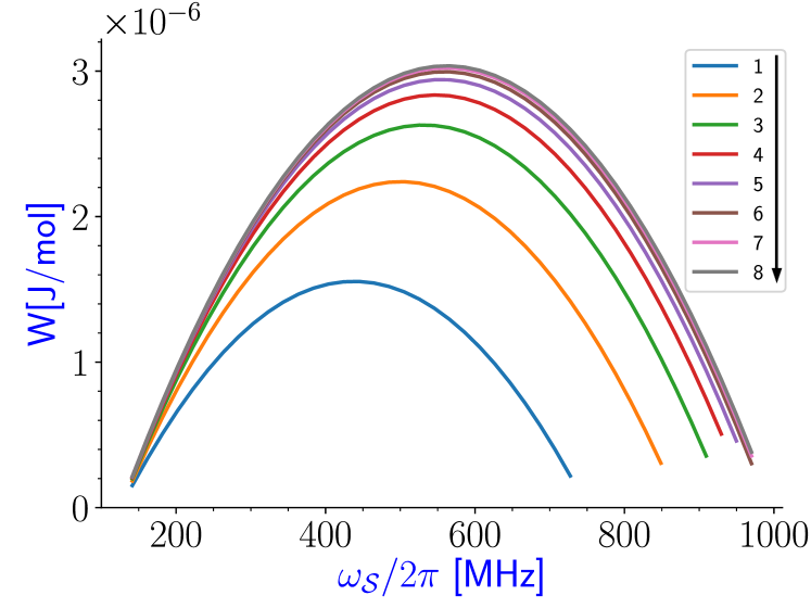
Figure 9: (Color online) Positive work obtained in 2 strokes HBAC-QOE as a function of $\omega_{\mathcal{S}}$. The legend of the plot shows the number of rounds of PPA applied to qubit $\mathcal{T}$ and direction of the arrow shows an increase in work output from 1st iteration to 8th iteration.

However, after some number of iteration, it remains almost constant, because of the limitation of PPA to cool qubit $\mathcal{T}$. It is found that for 580 MHz, we almost get the best work output at 5th and more iterations as $\sim 3.0\times 10^{-6}$ J/mol. But this frequency does not give us the best work output at 1st iteration, 430 MHz gives. For 1st iteration with 430 MHz frequency we get $\sim 1.5\times 10^{-6}$ J/mol work output. The adiabatic stage is evaluated by a SWAP operation, which is fast compared to the HBAC. Relaxation time of the $\mathcal{S}$ qubit may be estimated by considering spectral density functions $J(\omega,t_{c})$, where $t_{c}$ is the correlation time Redfield (1957); Abragam (1963). If we look for the optimum power output, the $\omega_{\mathcal{S}}$ is close to the frequency of the $\mathcal{R}$ qubit. Considering environmental effects are the same, $t_{c}$ may be assumed to be close for the $\mathcal{R}$ and $\mathcal{S}$ qubit. As a result, we can say that the $\mathcal{S}$ qubit is thermalized until the HBAC process is complete. In addition, using isochoric cooling instead of HBAC to cool target qubit requires more time up to the 5th iteration of PPA, as we have shown in the Sec. III.1. Thus, estimation of the power output depends on the relaxation time of reset qubit and the number of rounds of PPA. Then, we can write power output as $P={W}/{\tau_{\mathcal{R}}(2n+1)}$. The relaxation time of Hydrogen ($\tau_{\mathcal{R}}$) is given in Table  1. We plot the power output of the cycle in Fig. 10.

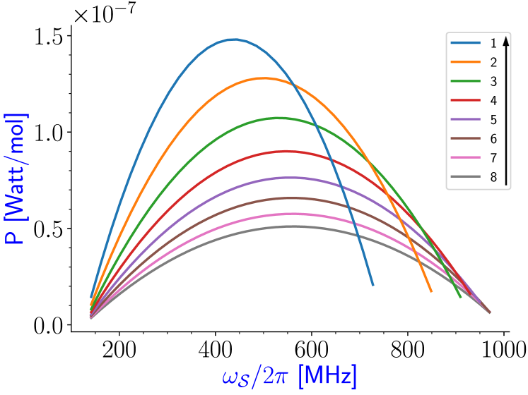
Figure 10: (Color online) Power output obtained in a two-stroke quantum Otto cycle for the different number of iterations of PPA as a function of $\omega_{\mathcal{S}}$. The legend of the plot shows the number of rounds of PPA applied to qubit $\mathcal{T}$ and the direction of the arrow shows an increase in the power output from 8th iteration to 1st iteration.

When the number of iterations increased, the power output is decreased despite the increase in the work output. The optimum value given by 1st iteration with 430 MHz frequency of $\mathcal{S}$ qubit as $\sim 1.47\times 10^{-7}$ Watt/mol. If we compare these results to four-stroke QOEs both cooled by HBAC and isochoric stage, we see that two stroke cycle gives more work and power output. The efficiency of the cycle as a function of $\omega_{\mathcal{S}}$ is given above. Taking the optimum value for the power output at 1st iteration and 430 MHz frequency of $\mathcal{S}$ qubit, the efficiency of the cycle is 0.7, which also more efficient than four-stroke QOEs.

IV CONCLUSIONS

We have investigated the possible quantum Otto engines considering HBAC instead of isochoric cooling. In conventional NMR setups do not let to change strength (huge) magnetic field along the z direction. In order to solve this restriction, NMR setup can be modified to change strong magnetic field via gradient coils such as Magnetic Resonance Imaging (MRI) system. In addition, the sample always in a single entropy sink in NMR systems. This is the main problem to design QOEs, which requires two heat bath to extract work from NMR qubits. Using HBAC allowed us to cool the working fluid in a single heat bath. Here we specifically showed this cooling process can be implemented to four-stroke and two-stroke QOEs. The isochoric cooling process of the cycle takes too much time compared to the HBAC. Comparing our results with a single spin NMR heat engine, utilizing the HBAC to QOEs improves the power output of the cycles up to a certain iteration of PPA.

Appendix A

A.1 Heat Bath Algorithmic Cooling - Partner Pairing Algorithm(PPA)

We consider heat bath algorithmic cooling (HBAC) with partner pairing algorithm (PPA) (see Fig. 11), which uses quantum information processing to increase the purification level of qubits in NMR systems Rodríguez-Briones and Laflamme (2016); Park et al. (2016).

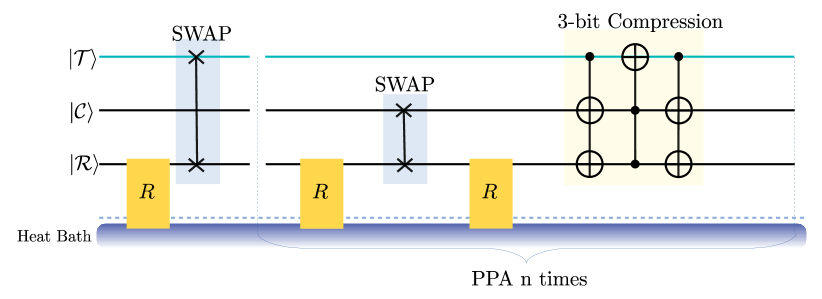
Figure 11: Quantum circuit demonstating partner pairing algorithm for 3-qubit system given in Ref. Rodríguez-Briones and Laflamme (2016). $|\mathcal{T}\rangle$, $|\mathcal{C}\rangle$ and $|\mathcal{R}\rangle$ stands for target, compression and reset qubits respectively. R process means the relaxation of reset qubit. In PPA, the first reset process applied only one time. Then, the iteration part consists of SWAP and 3-bit compression operations applied n times.

Before starting PPA, the individual density matrices of the target, the compression and the reset qubits are $\rho_{\mathcal{T}}^{(1)}=\mathrm{Tr}_{{\mathcal{C,R}}}\left[\rho^{(1)}\right]$, $\rho_{\mathcal{C}}^{(1)}=\mathrm{Tr}_{{\mathcal{T,R}}}\left[\rho^{(1)}\right]$, $\rho_{\mathcal{R}}^{(1)}=\mathrm{Tr}_{{\mathcal{T,C}}}\left(\rho^{(1)}\right)$ respectively and $\rho^{(1)}$ is the initial density matrix of 3-qubit system. The reset has small relaxation time compared to the target ($\tau_{R}\ll\tau_{T}$) and the compression ($\tau_{R}\ll\tau_{C}$) qubit, where $\tau_{\mathcal{T}},\tau_{\mathcal{C}}$ and $\tau_{\mathcal{R}}$ are given in Table 1 respectively. In each step of HBAC, $R$ operation is applied to the reset qubit to thermalize it with the heat bath $(\rho^{(1)}_{\mathcal{R}}\rightarrow\rho^{(1)}_{\mathcal{R},{th}})$ at temperature T. Scalar couplings between qubits are small compared to $\omega_{i}$ values. If we write the total density matrix of three qubits as a tensor product of the individual states, the fidelity of the density matrix in Eq. 2 and this product density matrix numerically is found to be close to 1. Thus, at first step, the density matrix of 3-qubit system can be written as a tensor product of these states

$$\rho^{(1,0)}_{AC}=\rho_{\mathcal{T}}^{(1)}\otimes\rho_{\mathcal{C}}^{(1)}\otimes\rho^{(1)}_{\mathcal{R},{th}},$$ (15)

where, 1st index of $\rho^{(1,0)}_{AC}$ stands for stage of the cycle and 2nd index from 0 to 5 indicates the state after each process of HBAC. After the reset qubit regains its polarization, a unitary SWAP operator is used to exchange polarizations of the target and the reset qubit.

$$\rho^{(1,1)}_{AC}=\mathrm{SWAP}_{\mathcal{T,R}}\left(\rho^{(1,0)}_{AC}\right)\mathrm{SWAP}_{\mathcal{T,R}}^{\dagger}$$ (16)

The states of the target and compression qubits become $\rho_{\mathcal{T}}^{(1,1)}=\mathrm{Tr}_{{\mathcal{C,R}}}\left[\rho^{(1,1)}_{AC}\right]$ and $\rho_{C}^{(1,1)}=\mathrm{Tr}_{{\mathcal{T,R}}}\left[\rho^{(1,1)}_{AC}\right]$ respectively. After the unitary evolution, PPA can be applied n times, which is given as follows

1. The reset qubit is thermalized with the heat bath. The density matrix of the 3-qubit system becomes

   $$\rho^{(1,2)}_{AC}=\rho_{\mathcal{T}}^{(1,1)}\otimes\rho_{\mathcal{C}}^{(1,1)}\otimes\rho^{(1)}_{\mathcal{R},{th}}$$ (17)

2. SWAP is applied to change polarization between the compression and the reset qubit, such that

   $$\rho^{(1,3)}_{AC}=\mathrm{SWAP}_{\mathcal{{C,R}}}\left(\rho^{(1,2)}_{AC}\right)\mathrm{SWAP}_{\mathcal{C,R}}^{\dagger}$$ (18)

   Then, the states of the target and the compression qubits becomes $\rho_{\mathcal{T}}^{(1,3)}=\mathrm{Tr}_{{\mathcal{C,R}}}\left[\rho^{(1,3)}_{AC}\right]$ and $\rho_{C}^{(1,3)}=\mathrm{Tr}_{{\mathcal{T,R}}}\left[\rho^{(1,3)}_{AC}\right]$.

3. The reset qubit is regained its polarization. The state of 3-qubit system is expressed as

   $$\rho^{(1,4)}_{AC}=\rho_{\mathcal{T}}^{(1,3)}\otimes\rho_{\mathcal{C}}^{(1,3)}\otimes\rho^{(1)}_{\mathcal{R},{th}}.$$ (19)

4. To lower the entropy of the target qubit and to increase the entropy of the reset qubit 3-bit compression gate applied to the density matrix.

   $$\rho^{(1,5)}_{AC}=\mathrm{COMP}\left(\rho^{(1,4)}_{AC}\right)\mathrm{COMP}^{\dagger}$$ (20)

   where COMP is the unitary operation of compression gate composed of unitary operators as two control-not-not gates and a Toffoli gate, which can be expressed as

   $$\mathrm{COMP=[CNotNot][Toffoli][CNotNot]}.$$ (21)

At the end of this iterative step the target qubit is cooled and the density matrix of it becomes

$$\rho^{(2)}_{\mathcal{T}}=\mathrm{Tr}_{\mathcal{C,R}}\left[\rho^{(1,5)}_{AC}\right].$$ (22)

References

- Quan et al. (2007) H. T. Quan, Yu-xi Liu, C. P. Sun, and Franco Nori, “Quantum thermodynamic cycles and quantum heat engines,” Phys. Rev. E 76, 031105 (2007).
- Huang et al. (2014) Xiao-Li Huang, Xin-Ya Niu, Xiao-Ming Xiu, and Xue-Xi Yi, “Quantum stirling heat engine and refrigerator with single and coupled spin systems,” The European Physical Journal D 68, 32 (2014).
- Thomas and Johal (2014) George Thomas and Ramandeep S. Johal, “Friction due to inhomogeneous driving of coupled spins in a quantum heat engine,” The European Physical Journal B 87, 166 (2014).
- Zhang et al. (2007) Ting Zhang, Wei-Tao Liu, Ping-Xing Chen, and Cheng-Zu Li, “Four-level entangled quantum heat engines,” Phys. Rev. A 75, 062102 (2007).
- Huang et al. (2013) X L Huang, Huan Xu, X Y Niu, and Y D Fu, “A special entangled quantum heat engine based on the two-qubit heisenberg xx model,” Physica Scripta 88, 065008 (2013).
- Thomas and Johal (2011) George Thomas and Ramandeep S. Johal, “Coupled quantum otto cycle,” Phys. Rev. E 83, 031135 (2011).
- Scully et al. (2003) Marlan O. Scully, M. Suhail Zubairy, Girish S. Agarwal, and Herbert Walther, “Extracting work from a single heat bath via vanishing quantum coherence,” Science (2003), 10.1126/science.1078955.
- Zhang (2008) G. F. Zhang, “Entangled quantum heat engines based on two two-spin systems with dzyaloshinski-moriya anisotropic antisymmetric interaction,” The European Physical Journal D 49, 123 (2008).
- Çakmak et al. (2016) Selçuk Çakmak, Ferdi Altintas, and Özgür E. Müstecaplıoğlu, “Lipkin-meshkov-glick model in a quantum otto cycle,” The European Physical Journal Plus 131, 197 (2016).
- Zhang et al. (2014) Keye Zhang, Francesco Bariani, and Pierre Meystre, “Quantum optomechanical heat engine,” Phys. Rev. Lett. 112, 150602 (2014).
- Türkpençe and Müstecaplıoğlu (2016) Deniz Türkpençe and Özgür E. Müstecaplıoğlu, “Quantum fuel with multilevel atomic coherence for ultrahigh specific work in a photonic carnot engine,” Phys. Rev. E 93, 012145 (2016).
- Chand and Biswas (2017a) Suman Chand and Asoka Biswas, “Single-ion quantum otto engine with always-on bath interaction,” EPL (Europhysics Letters) 118, 60003 (2017a).
- Chand and Biswas (2017b) Suman Chand and Asoka Biswas, “Measurement-induced operation of two-ion quantum heat machines,” Phys. Rev. E 95, 032111 (2017b).
- Uzdin et al. (2015) Raam Uzdin, Amikam Levy, and Ronnie Kosloff, “Equivalence of quantum heat machines, and quantum-thermodynamic signatures,” Phys. Rev. X 5, 031044 (2015).
- Alecce et al. (2015) A. Alecce, F. Galve, N. Lo Gullo, L. Dell’Anna, F. Plastina, and R. Zambrini, “Quantum Otto cycle with inner friction: Finite-time and disorder effects,” New J. Phys. 17 (2015), 10.1088/1367-2630/17/7/075007, 1507.03417 .
- Scovil and Schulz-DuBois (1959) H. E. D. Scovil and E. O. Schulz-DuBois, “Three-level masers as heat engines,” Phys. Rev. Lett. 2, 262–263 (1959).
- Alicki (1979) R Alicki, “The quantum open system as a model of the heat engine,” Journal of Physics A: Mathematical and General 12, L103 (1979).
- Linden et al. (2010) Noah Linden, Sandu Popescu, and Paul Skrzypczyk, “How small can thermal machines be? the smallest possible refrigerator,” Phys. Rev. Lett. 105, 130401 (2010).
- Uzdin and Kosloff (2014) Raam Uzdin and Ronnie Kosloff, “The multilevel four-stroke swap engine and its environment,” New Journal of Physics 16, 095003 (2014).
- Gelbwaser-Klimovsky et al. (2013) D. Gelbwaser-Klimovsky, R. Alicki, and G. Kurizki, “Minimal universal quantum heat machine,” Phys. Rev. E 87, 012140 (2013).
- Kosloff and Levy (2014) Ronnie Kosloff and Amikam Levy, “Quantum heat engines and refrigerators: Continuous devices,” Annual Review of Physical Chemistry 65, 365–393 (2014), pMID: 24689798.
- Feldmann and Kosloff (2003) Tova Feldmann and Ronnie Kosloff, “Quantum four-stroke heat engine: Thermodynamic observables in a model with intrinsic friction,” Phys. Rev. E 68, 016101 (2003).
- Roßnagel et al. (2016) Johannes Roßnagel, Samuel T. Dawkins, Karl N. Tolazzi, Obinna Abah, Eric Lutz, Ferdinand Schmidt-Kaler, and Kilian Singer, “A single-atom heat engine,” Science 352, 325–329 (2016), http://science.sciencemag.org/content/352/6283/325.full.pdf .
- Abah et al. (2012) O. Abah, J. Roßnagel, G. Jacob, S. Deffner, F. Schmidt-Kaler, K. Singer, and E. Lutz, “Single-ion heat engine at maximum power,” Phys. Rev. Lett. 109, 203006 (2012).
- Klaers et al. (2017) Jan Klaers, Stefan Faelt, Atac Imamoglu, and Emre Togan, “Squeezed thermal reservoirs as a resource for a nanomechanical engine beyond the carnot limit,” Phys. Rev. X 7, 031044 (2017).
- Roßnagel et al. (2014) J. Roßnagel, O. Abah, F. Schmidt-Kaler, K. Singer, and E. Lutz, “Nanoscale heat engine beyond the carnot limit,” Phys. Rev. Lett. 112, 030602 (2014).
- Dillenschneider and Lutz (2009) R. Dillenschneider and E. Lutz, “Energetics of quantum correlations,” EPL (Europhysics Letters) 88, 50003 (2009).
- Dağ et al. (2016) Ceren B. Dağ, Wolfgang Niedenzu, Özgür E. Müstecaplioğlu, and Gershon Kurizki, “Multiatom quantum coherences in micromasers as fuel for thermal and nonthermal machines,” Entropy 18, 244 (2016).
- Peterson et al. (2018) John P. S. Peterson, Tiago B. Batalhão, Marcela Herrera, Alexandre M. Souza, Roberto S. Sarthour, Ivan S. Oliveira, and Roberto M. Serra, “Experimental characterization of a spin quantum heat engine,” (2018), arXiv:1803.06021 .
- De Assis et al. (2018) Rogério J De Assis, Taysa M De Mendonça, Celso J Villas-Boas, Alexandre M De Souza, Roberto S Sarthour, Ivan S Oliveira, and Norton G De Almeida, “Quantum heating engine beating the Otto limit,” (2018), arXiv:1811.02917v1 .
- Çakmak et al. (2017) Selçuk Çakmak, Ferdi Altintas, Azmi Gençten, and Özgür E. Müstecaplıoğlu, “Irreversible work and internal friction in a quantum otto cycle of a single arbitrary spin,” The European Physical Journal D 71, 75 (2017).
- Park et al. (2016) Daniel K. Park, Nayeli A. Rodriguez-Briones, Guanru Feng, Robabeh Rahimi, Jonathan Baugh, and Raymond Laflamme, “Heat bath algorithmic cooling with spins: Review and prospects,” in Electron Spin Resonance (ESR) Based Quantum Computing, edited by Takeji Takui, Lawrence Berliner, and Graeme Hanson (Springer New York, New York, NY, 2016) pp. 227–255.
- Rodríguez-Briones and Laflamme (2016) Nayeli Azucena Rodríguez-Briones and Raymond Laflamme, “Achievable polarization for heat-bath algorithmic cooling,” Phys. Rev. Lett. 116, 170501 (2016).
- Atia et al. (2016) Yosi Atia, Yuval Elias, Tal Mor, and Yossi Weinstein, “Algorithmic cooling in liquid-state nuclear magnetic resonance,” Phys. Rev. A 93, 012325 (2016).
- Brassard et al. (2014a) G. Brassard, Y. Elias, J. M. Fernandez, H. Gilboa, J. A. Jones, T. Mor, Y. Weinstein, and L. Xiao, “Experimental heat-bath cooling of spins,” The European Physical Journal Plus 129, 266 (2014a).
- Brassard et al. (2014b) Gilles Brassard, Yuval Elias, Tal Mor, and Yossi Weinstein, “Prospects and limitations of algorithmic cooling,” The European Physical Journal Plus 129, 258 (2014b).
- Fernandez et al. (2004) Jose M. Fernandez, Seth Lloyd, Tal Mor, and Vwani Roychowdhury, “Algorithmic Cooling of Spins: A Practicable Method for Increasing Polarization,” Int. J. Quantum Inf. 02, 461–477 (2004).
- Elias et al. (2007) Yuval Elias, José M. Fernandez, Tal Mor, and Yossi Weinstein, Unconv. Comput., edited by Selim G. Akl, Cristian S. Calude, Michael J. Dinneen, Grzegorz Rozenberg, and H. Todd Wareham, Lecture Notes in Computer Science, Vol. 4618 (Springer Berlin Heidelberg, Berlin, Heidelberg, 2007) pp. 2–26, 0711.2964 .
- Boykin et al. (2002) P. Oscar Boykin, Tal Mor, Vwani Roychowdhury, Farrokh Vatan, and Rutger Vrijen, “Algorithmic cooling and scalable nmr quantum computers,” Proceedings of the National Academy of Sciences 99, 3388–3393 (2002), http://www.pnas.org/content/99/6/3388.full.pdf .
- Kafri and Taylor (2012) Dvir Kafri and Jacob M. Taylor, “Algorithmic Cooling of a Quantum Simulator,” , 41 (2012), 1207.7111 .
- Raeisi and Mosca (2015) Sadegh Raeisi and Michele Mosca, “Asymptotic bound for heat-bath algorithmic cooling,” Phys. Rev. Lett. 114, 100404 (2015).
- Rodríguez-Briones et al. (2017) Nayeli A. Rodríguez-Briones, Jun Li, Xinhua Peng, Tal Mor, Yossi Weinstein, and Raymond Laflamme, “Heat-bath algorithmic cooling with correlated qubit-environment interactions,” New J. Phys. 19 (2017), 10.1088/1367-2630/aa8fe0.
- Ryan et al. (2008) C. A. Ryan, O. Moussa, J. Baugh, and R. Laflamme, “Spin based heat engine: Demonstration of multiple rounds of algorithmic cooling,” Phys. Rev. Lett. 100, 140501 (2008).
- Schulman et al. (2005) Leonard J. Schulman, Tal Mor, and Yossi Weinstein, “Physical limits of heat-bath algorithmic cooling,” Phys. Rev. Lett. 94, 120501 (2005).
- Elias et al. (2006) Yuval Elias, José M. Fernandez, Tal Mor, and Yossi Weinstein, “Optimal Algorithmic Cooling of Spins,” Isr. J. Chem. 46, 371–391 (2006).
- Oliveira et al. (2007) Ivan S. Oliveira, Tito J. Bonagamba, Roberto S. Sarthour, Jair C.C. Freitas, and Eduardo R. deAzevedo, “4 - introduction to nmr quantum computing,” in NMR Quantum Information Processing (Elsevier Science B.V., Amsterdam, 2007) pp. 137 – 181.
- Devoret et al. (2011) M. Devoret, B. Huard, R. Schoelkopf, and L.F. Cugliandolo, Quantum Machines: Measurement and Control of Engineered Quantum Systems (2011).
- Abragam (1963) A Abragam, “Principles of nuclear magnetism,” Am. J. Phys. (1963), 10.1016/0029-5582(61)90091-8.
- Goold et al. (2016) John Goold, Marcus Huber, Arnau Riera, Lídia del Rio, and Paul Skrzypczyk, “The role of quantum information in thermodynamics—a topical review,” Journal of Physics A: Mathematical and Theoretical 49, 143001 (2016).
- Batalhão et al. (2014) Tiago B. Batalhão, Alexandre M. Souza, Laura Mazzola, Ruben Auccaise, Roberto S. Sarthour, Ivan S. Oliveira, John Goold, Gabriele De Chiara, Mauro Paternostro, and Roberto M. Serra, “Experimental reconstruction of work distribution and study of fluctuation relations in a closed quantum system,” Phys. Rev. Lett. 113, 140601 (2014).
- Hou et al. (2014) Shi Yao Hou, Yu Bo Sheng, Guan Ru Feng, and Gui Lu Long, “Experimental optimal single qubit purification in an NMR quantum information processor,” Sci. Rep. 4 (2014), 10.1038/srep06857.
- Li et al. (2011) Zhaokai Li, Man Hong Yung, Hongwei Chen, Dawei Lu, James D. Whitfield, Xinhua Peng, Alán Aspuru-Guzik, and Jiangfeng Du, “Solving quantum ground-state problems with nuclear magnetic resonance,” Sci. Rep. 1 (2011), 10.1038/srep00088.
- Henry et al. (2006) Michael K. Henry, Joseph Emerson, Rudy Martinez, and David G. Cory, “Localization in the quantum sawtooth map emulated on a quantum-information processor,” Phys. Rev. A 74, 062317 (2006).
- Cummins et al. (2002) Holly K. Cummins, Claire Jones, Alistair Furze, Nicholas F. Soffe, Michele Mosca, Josephine M. Peach, and Jonathan A. Jones, “Approximate quantum cloning with nuclear magnetic resonance,” Phys. Rev. Lett. 88, 187901 (2002).
- Kosloff (2013) Ronnie Kosloff, “Quantum thermodynamics: A dynamical viewpoint,” Entropy 15, 2100–2128 (2013).
- Vinjanampathy and Anders (2016) Sai Vinjanampathy and Janet Anders, “Quantum thermodynamics,” Contemporary Physics 57, 545–579 (2016).
- Redfield (1957) A. G. Redfield, “On the theory of relaxation processes,” IBM Journal of Research and Development 1, 19–31 (1957).