Intelligent Intersection: Two-Stream Convolutional Networks for Real-time Near Accident Detection in Traffic Video

Abstract.

In Intelligent Transportation System, real-time systems that monitor and analyze road users become increasingly critical as we march toward the smart city era. Vision-based frameworks for Object Detection, Multiple Object Tracking, and Traffic Near Accident Detection are important applications of Intelligent Transportation System, particularly in video surveillance and etc. Although deep neural networks have recently achieved great success in many computer vision tasks, a uniformed framework for all the three tasks is still challenging where the challenges multiply from demand for real-time performance, complex urban setting, highly dynamic traffic event, and many traffic movements. In this paper, we propose a two-stream Convolutional Network architecture that performs real-time detection, tracking, and near accident detection of road users in traffic video data. The two-stream model consists of a spatial stream network for Object Detection and a temporal stream network to leverage motion features for Multiple Object Tracking. We detect near accidents by incorporating appearance features and motion features from two-stream networks. Using aerial videos, we propose a Traffic Near Accident Dataset (TNAD) covering various types of traffic interactions that is suitable for vision-based traffic analysis tasks. Our experiments demonstrate the advantage of our framework with an overall competitive qualitative and quantitative performance at high frame rates on the TNAD dataset.

1. Introduction

The technologies of Artificial Intelligence (AI) and Internet of Things (IoTs) are ushering in a new promising era of ”Smart Cities”, where billions of people around the world can improve the quality of their life in aspects of transportation, security, information and communications and etc. One example of the data-centric AI solutions is computer vision technologies that enables vision-based intelligence at the edge devices across multiple architectures. Sensor data from smart devices or video cameras can be analyzed immediately to provide real-time analysis for the Intelligent Transportation System (ITS). At traffic intersections, it has more volume of road users (pedestrians, vehicles), traffic movement, dynamic traffic event, near accidents and etc. It is a critically important application to enable global monitoring of traffic flow, local analysis of road users, automatic near accident detection.

As a new technology, vision-based intelligence has a wide range of applications in traffic surveillance and traffic management (Coifman et al., 1998; Valera and Velastin, 2005; Buch et al., 2011; Kamijo et al., 2000; Veeraraghavan et al., 2003; He et al., 2017). Among them, many research works have focused on traffic data acquirement with aerial videos (Angel et al., 2002; Salvo et al., 2017), where the aerial view provides better perspectives to cover a large area and focus resources for surveillance tasks. Unmanned Aerial Vehicles (UAVs) and omnidirectional cameras can acquire useful aerial videos for traffic surveillance especially at intersections with a broader perspective of the traffic scene, with the advantage of being both mobile, and able to be present in both time and space. UAVs has been exploited in a wide range of transportation operations and planning applications including emergency vehicle guidance, track vehicle movements. A recent trend of vision-based intelligence is to apply computer vision technologies to these acquired intersection aerial videos  (Scotti et al., 2005; Wang et al., 2006) and process them at the edge across multiple ITS architecture.

From global monitoring of traffic flow for solving traffic congestion to quest for better traffic information, an increasing reliance of ITS has resulted in a need for better object detection (such as wide-area detectors for pedestrian, vehicles), and multiple vehicle tracking that yields traffic parameters such as flow, velocity and vehicle trajectories. Tracks and trajectories are measures over a length of path rather than at a single point. It is possible to tackle related surveillance tasks including traffic movement measurements (e.g. turn movement counting) and routing information. The additional information from vehicle trajectories could be utilized to improve near accident detection, by either detecting stopped vehicles with their collision status or identifying acceleration / deceleration patterns or conflicting trajectories that are indicative of near accidents. Based on the trajectories, it is also possible to learn and forecast vehicle trajectory to enable near accident anticipation.

Generally, a vision-based surveillance tool for intelligent transportation system should meet several requirements:

1. Segment vehicles from the background and from other vehicles so that all vehicles (stopped or moving) are detected;

2. Classify detected vehicles into categories: cars, buses, trucks, motorcycles and etc;

3. Extract spatial and temporal features (motion, velocity, trajectory) to enable more specific tasks including vehicle tracking, trajectory analysis, near accident detection, anomaly detection and etc;

4. Function under a wide range of traffic conditions (light traffic, congestion, varying speeds in different lanes) and a wide variety of lighting conditions (sunny, overcast, twilight, night, rainy, etc.);

5. Operate in real-time.

Over the decades, although an increasing number of research on vision-based system for traffic surveillance have been proposed, many of these criteria still cannot be met. Early solutions (Hoose, 1992) do not identify individual vehicles as unique targets and progressively track their movements. Methods have been proposed to address individual vehicle detection and vehicles tracking problems (Koller et al., 1993; McLauchlan et al., 1997; Coifman et al., 1998) with tracking strategies including model based tracking, region based tracking, active contour based tracking, feature based tracking and optical flow employment. Compared to traditional hand-crafted features, deep learning methods (Ren et al., 2015; Girshick et al., 2016; Redmon et al., 2016; Tian et al., 2016) in object detection have illustrated the robustness with specialization of the generic detector to a specific scene. Leuck (Leuck and Nagel, 1999) and Gardner (Gardner and Lawton, 1996) use three-dimensional (3-D) models of vehicle shapes to estimate vehicle images projected onto a two-dimensional (2-D) image plane. Recently, automatic traffic accident detection has become an important topic. One typical approach uses object detection or tracking before detecting accident events (Sadeky et al., 2010; Kamijo et al., 2000; Jiansheng et al., 2014; Jiang et al., 2007; Hommes et al., 2011), with Histogram of Flow Gradient (HFG), Hidden Markov Model (HMM) or, Gaussian Mixture Model (GMM). Other approaches (Liu et al., 2010; Ihaddadene and Djeraba, 2008; Wang and Miao, 2010; Wang and Dong, 2012; Tang and Gao, 2005; Karim and Adeli, 2002; Xia et al., 2015; Chen et al., 2010, 2016) use low-level features (e.g. motion features) to demonstrate better robustness. Neural networks have also been employed to automatic accident detection (Ohe et al., 1995; Yu et al., 2008; Srinivasan et al., 2004; Ghosh-Dastidar and Adeli, 2003).

In this paper, we first propose a Traffic Near Accident Dataset (TNAD). Intersections tend to experience more and severe near accident, due to factors such as angles and turning collisions. Observing this, the TNAD dataset is collected to contain three types of video data of traffic intersections that could be utilized for not only near accident detection but also other traffic surveillance tasks including turn movement counting. The first type is drone video that monitoring an intersections with top-down view. The second type of intersection videos is real traffic videos acquired by omnidirectional fisheye cameras that monitoring small or large intersections. It is widely used in transportation surveillance. These video data can be directly used as inputs for any vision-intelligent framework. The pre-processing of fisheye correction can be applied to them for better surveillance performance. As there exist only a few samples of near accident in the reality per hour. The third type of video is proposed by simulating with game engine for the purpose to train and test with more near accident samples.

We propose a uniformed vision-based framework with the two-stream Convolutional Network architecture that performs real-time detection, tracking, and near accident detection of traffic road users. The two-stream Convolutional Networks consist of a spatial stream network to detect individual vehicles and likely near accident regions at the single frame level, by capturing appearance features with a state-of-the-art object detection method (Redmon et al., 2016). The temporal stream network leverages motion features extracted from detected candidates to perform multiple object Tracking and generate corresponding trajectories of each tracking target. We detect near accident by incorporating appearance features and motion features to compute probabilities of near accident candidate regions. Experiments demonstrate the advantage of our framework with an overall competitive performance at high frame rates. The contributions of this work can be summarized as:

• A uniformed framework that performs real-time object detection, tracking and near accident detection.

• The first work of an end-to-end trainable two-stream deep models to detect near accident with good accuracy.

• A Traffic and Near Accident Detection Dataset (TNAD) containing different types of intersection videos that would be used for several vision-based traffic analysis tasks.

The organization of the paper is as follows. Section 2 describes background on Object Detection, Multiple Object Tracking and Near Accident Detection. Section 3 describes the overall architecture, methodologies, and implementation of our vision-based intelligent framework. This is followed in Section 4 by an introduction of our Traffic Near Accident Detection Dataset (TNAD) and video preprocessing techniques. Section 4 presents a comprehensive evaluation of our approach and other state-of-the-art near accident detection methods both qualitatively and quantitatively. Section 5 concludes by summarizing our contributions and also discusses the scope for future work.

2. Background

2.1. Object Detection

Object detection has received significant attention and achieved striking improvements in recent years, as demonstrated in popular object detection competitions such as PASCAL VOC detection challenge (Everingham et al., 2010, 2015a), ILSVRC large scale detection challenge (Russakovsky et al., 2015) and MS COCO large scale detection challenge (Lin et al., 2014). Object detection aims at outputting instances of semantic objects with a certain class label such as humans, cars. It has wide applications in many computer vision tasks including face detection, face recognition, pedestrian detection, video object co-segmentation, image retrieval, object tracking and video surveillance. Different from image classification, object detection is not to classify the whole image. Position and category information of the objects are both needed which means we have to segment instances of objects from backgrounds and label them with position and class. The inputs are images or video frames while the outputs are lists where each item represents position and category information of candidate objects. In general, object detection seeks to extract discriminative features to help in distinguishing the classes.

Methods for object detection generally fall into 3 categories: 1) traditional machine learning based approaches; 2) region proposal based deep learning approaches; 3) end-to-end deep learning approaches. For traditional machine learning based approaches, one of the important steps is to design features. Many methods have been proposed to first design features (Viola and Jones, 2001, 2004; Lowe, 1999; Dalal and Triggs, 2005) and apply techniques such as support vector machine (SVM) (Hearst et al., 1998) to do the classification. The main steps of traditional machine learning based approaches are:

• Region Selection: using sliding windows at different sizes to select candidate regions from whole images or video frames;

• Feature Extraction: extract visual features from candidate regions using techniques such as Harr feature for face detection, HOG feature for pedestrian detection or general object detection;

• Classifier: train and test classifier using techniques such as SVM.

The tradition machine learning based approaches have their limitations. The scheme using sliding windows to select RoIs (Regions of Interests) increases computation time with a lot of window redundancies. On the other hand, these hand-crafted features are not robust due to the diversity of objects, deformation, lighting condition, background and etc., while the feature selection has a huge effect on classification performance of candidate regions.

Recent advances in deep learning, especially in computer vision have shown that Convolutional Neural Networks (CNNs) have a strong capability of representing objects and help to boost the performance of numerous vision tasks, comparing to traditional heuristic features (Dalal and Triggs, 2005). For deep learning based approaches, there are convolutional neural networks (CNN) to extract features of region proposals or end-to-end object detection without specifically defining features of a certain class. The well-performed deep learning based approaches of object detection includes Region Proposals (R-CNN) (Girshick et al., 2014), Fast R-CNN (Girshick, 2015), Faster R-CNN (Ren et al., 2015)), Single Shot MultiBox Detector (SSD) (Liu et al., 2016), and You Only Look Once (YOLO) (Redmon et al., 2016).

Usually, we adopt region proposal methods (Category 2) for producing multiple object proposals, and then apply a robust classifier to further refine the generated proposals, which are also referred as two-stage method. The first work of the region proposal based deep learning approaches is R-CNN (Girshick et al., 2014) proposed to solve the problem of selecting a huge number of regions. The main pipeline of R-CNN (Girshick et al., 2014) is: 1) gathering input images; 2) generating a number of region proposals (e.g. 2000); 3) extracting CNN features; 4) classifying regions using SVM. It usually adopts Selective Search (SS), one of the state-of-art object proposals method (Uijlings et al., 2013) applied in numerous detection task on several fascinating systems(Girshick et al., 2014; Girshick, 2015; Ren et al., 2015), to extract these regions from the image and names them region proposals. Instead of trying to classify all the possible proposals, R-CNN select a fixed set of proposals (e.g. 2000) to work with. The selective search algorithm used to generate these region proposals includes: (1) Generate initial sub-segmentation, generate many candidate regions; (2) Use greedy algorithm to recursively combine similar regions into larger ones; (3) Use the generated regions to produce the final candidate region proposals.

These candidate region proposals are warped into a square and fed into a convolutional neural network (CNN) which acts as the feature extractor. The output dense layer consists of the extracted features to be fed into an SVM (Hearst et al., 1998) to classify the presence of the object within that candidate region proposal. The main problem of R-CNN (Girshick et al., 2014) is that it is limited by the inference speed, due to a huge amount of time spent on extracting features of each individual region proposal. And it cannot be applied in applications requiring a real-time performance (such as online video analysis). Later, Fast R-CNN (Girshick, 2015) is proposed to improve the speed by avoiding feeding raw region proposals every time. Instead, the convolution operation is done only once per image and RoIs over the feature map are generated. Faster R-CNN (Ren et al., 2015) further exploits the shared convolutional features to extract region proposals used by the detector. Sharing convolutional features leads to substantially faster speed for object detection system.

The third type is end-to-end deep learning approaches which do not need region proposals (also referred as one-stage method). The pioneer works are SSD (Liu et al., 2016) and YOLO (Redmon et al., 2016) . An SSD detector (Liu et al., 2016) works by adding a sequence of feature maps of progressively decreasing the spatial resolution to replace the two stage’s second classification stage, allowing a fast computation and multi-scale detection on one single input. YOLO detecor is an object detection algorithm much different from the region based algorithms. In YOLO (Redmon et al., 2016), it regards object detection as an end-to-end regression problem and uses a single convolutional network to predict the bounding boxes and the corresponding class probabilities. It first takes the image and splits it into an $S\times S$ grid, within each of the grid we take $m$ bounding boxes. For each of the bounding box with multi scales, the convolutional neural network outputs a class probability and offset values for the bounding box. Then it selects bounding boxes which have the class probability above a threshold value and uses them to locate the object within the image. YOLO (Redmon et al., 2016) is orders of magnitude faster (45 frames per second) than other object detection approaches but the limitation is that it struggles with small objects within the image.

2.2. Multiple Object Tracking

Video object tracking is to locate objects over video frames and it has various important applications in robotics, video surveillance and video scene understanding. Based on the number of moving objects that we wish to track, there are Single Object Tracking (SOT) problem and Multiple Object Tracking (MOT) problem. In addition to detecting objects in video frame, the MOT solution requires to robustly associate multiple detected objects between frames to get a consistent tracking and this data association part remains very challenging. In MOT tasks, for each frame in a video, we aim at localizing and identifying all objects of interests, so that the identities are consistent throughout the video. Typically, the main challenge lies on speed, data association, appearance change, occlusions, disappear / re-enter objects and etc. In practice, it is desired that the tracking could be performed in real-time so as to run as fast as the frame-rate of the video. Also, it is challenging to provide a consistent labeling of the detected objects in complex scenarios such as objects change appearance, disappear, or involve severe occlusions.

In general, Multiple Object Tracking (MOT) can be regarded as a multi-variable estimation problem (Luo et al., 2014). The objective of multiple object tracking can be modeled by performing MAP (maximal a posteriori) estimation in order to find the optimal sequential states of all the objects, from the conditional distribution of the sequential states given all the observations:

(1) $$\widehat{\mathbf{S}}_{1:t}=\underset{\mathbf{S}_{1:t}}{\operatorname{arg\,max}}\ P\left(\mathbf{S}_{1:t}|\mathbf{O}_{1:t}\right).$$

where $\mathbf{s}_{t}^{i}$ denotes the state of the $i$-th object in the $t$-th frame. $\mathbf{S}_{t}=(\mathbf{s}_{t}^{1},\mathbf{s}_{t}^{2},...,\mathbf{s}_{t}^{M_{t}})$ denotes states of all the $M_{t}$ objects in the $t$-th frame. $\mathbf{S}_{1:t}=\{\mathbf{S}_{1},\mathbf{S}_{2},...,\mathbf{S}_{t}\}$ denotes all the sequential states of all the objects from the first frame to the $t$-th frame. In tracking-by-detection, $\mathbf{o}_{t}^{i}$ denotes the collected observations for the $i$-th object in the $t$-th frame. $\mathbf{O}_{t}=(\mathbf{o}_{t}^{1},\mathbf{o}_{t}^{2},...,\mathbf{o}_{t}^{M_{t}})$ denotes the collected observations for all the $M_{t}$ objects in the $t$-th frame. $\mathbf{O}_{1:t}=\{\mathbf{O}_{1},\mathbf{O}_{2},...,\mathbf{O}_{t}\}$ denotes all the collected sequential observations of all the objects from the first frame to the $t$-th frame. Different Multiple Object Tracking (MOT) algorithms can be thought as designing different approaches to solving the above MAP problem, either from a probabilistic inference perspective, e.g. Kalman filter or a deterministic optimization perspective, e.g. Bipartite graph matching, and machine learning approaches.

Multiple Object Tracking (MOT) approaches can be categorized by different types of models. A distinction based on Initialization Method is that of Detection Based Tracking (DBT) versus Detection Free Tracking (DFT). DBT refers that before tracking, object detection is performed on video frames. DBT methods involve two distinct jobs between the detection and tracking of objects. In this paper, we focus on DBT, also refers as tracking-by-detection for MOT. The reason is that DBT methods are widely used due to excellent performance with deep learning based object detectors, while DFT methods require manually annotations of the targets and bad results could arise when a new unseen object appears. Another important distinction based on Processing Mode is that of Online versus Offline models. An Online model receives video input on a frame-by-frame basis, and gives output per frame. This means only information from past frames and the current frame can be used. Offline models have access to the entire video, which means that information from both past and future frames can be used.

Tracking-by-detection methods are usually utilized in online tracking models. A simple and classic pipeline is as (1) Detect objects of interest; (2) Predict new locations of objects from previous frames; (3) Associate objects between frames by similarity of detected and predicted locations. Well-performed CNN architectures can be used for object detection such as Faster R-CNN (Ren et al., 2015), YOLO (Redmon et al., 2016) and SSD (Liu et al., 2016). For prediction of new locations of tracked objects, approaches model the velocity of objects, and predict the position in future frames using optical flow, or recurrent neural networks, or Kalman filters. The association task is to determine which detection corresponds to which object, or a detection represents a new object.

One popular dataset for Multiple Object Tracking (MOT) is MOTChallenge (Leal-Taixé et al., 2015). In MOTChallenge (Leal-Taixé et al., 2015), detections for each frame are provided in the dataset, and the tracking capability is measured as opposed to the detection quality. Video sequences are labeled with bounding boxes for each pedestrian collected from multiple sources. This motivates the use of tracking-by-detection paradigm. MDPs (Xiang et al., 2015) is a tracking-by-detection method and achieved the state-of-the-art performance on MOTChallenge (Leal-Taixé et al., 2015) Benchmark when it was proposed. Major contributions can be solving MOT by learning a MDP policy in a reinforcement learning fashion which benefits from both advantages of offline-learning and online-learning for data association. It also can handle the birth / death and appearance / disappearance of targets by simply treating them as state transitions in the MDP while leveraging existing online single object tracking methods. SORT (Bewley et al., 2016) is a simple and real-time Multiple Object Tracking (MOT) method where state-of-the-art tracking quality can be achieved with only classical tracking methods. It is the most widely used real-time online Multiple Object Tracking (MOT) method and is very efficient for real-time applications in practice. Due to the simplicity of SORT (Bewley et al., 2016), the tracker updates at a rate of 260 Hz which is over 20x faster than other state-of-the-art trackers. On the MOTChallenge (Leal-Taixé et al., 2015), SORT (Bewley et al., 2016) with a state-of-the-art people detector ranks on average higher than MHT (Kim et al., 2015) on standard detections. DeepSort (Wojke et al., 2017) is an extension of SORT (Bewley et al., 2016) which integrates appearance information to improve the performance of SORT (Bewley et al., 2016) which can track through longer periods of occlusion, making SORT (Bewley et al., 2016) a strong competitor to state-of-the-art online tracking algorithms.

2.3. Near Accident Detection

In addition to vehicle detection and vehicle tracking, analysis of the interactions or behavior of tracked vehicles has emerged as an active and challenging research area in recent years (Sivaraman et al., 2011; Hermes et al., 2009; Wiest et al., 2012). Near Accident Detection is one of the highest levels of semantic interpretation in characterizing the interactions of vehicles on the road. The basic task of near accident detection is to locate near accident regions and report them over video frames. In order to detect near accident on traffic scenes, robust vehicle detection and vehicle tracking are the prerequisite tasks.

Most of the near accident detection approaches are based on motion cues and trajectories. The most typical motion cues are optical flow and trajectory. Optical flow is widely utilized in video processing tasks such as video segmentation (Huang et al., 2018). A trajectory is defined as a data sequence containing several concatenated state vectors from tracking, an indexed sequence of positions and velocities over a given time window. In recent years, researches have tried to make long-term classification and prediction of vehicle motion. Based on vehicle tracking algorithms such as Kalman filtering, optimal estimation of the vehicle state can be computed one frame ahead of time. Trajectory modeling approaches try to predict vehicle motion more frames ahead of time, based on models of typical vehicle trajectories (Sivaraman et al., 2011; Hermes et al., 2009; Wiest et al., 2012). In (Sivaraman et al., 2011), it used clustering to model the typical trajectories in highway driving and hidden Markov modeling for classification. In (Hermes et al., 2009), trajectories are classified using a rotation-invariant version of the longest common subsequence as the similarity metric between trajectories. In (Wiest et al., 2012), it uses variational Gaussian mixture modeling to classify and predict the long-term trajectories of vehicles.

Over the past two decades, for automatic traffic accident detection, a great deal of literature emerged in various ways. Several approaches have been developed based on decision trees, Kalman filters, or time series analysis, with varying degrees of success in their performance (Srinivasan et al., 2003, 2001; Xu et al., 1998; Shuming et al., 2002; Jiansheng et al., 2014; Bhonsle et al., 2000). Ohe et al. (Ohe et al., 1995) use neural networks to detect traffic incidents immediately by utilizing one minute average traffic data as input, and determine whether an incident has occurred or not. In (Ikeda et al., 1999), the authors propose a system to distinguish between different types of incidents for automatic incident detection. In (Kimachi et al., 1994), it investigates the abnormal behavior of vehicle related to accident based on the concepts of fuzzy theory where accident occurrence relies on the behavioral abnormality of multiple continual images. Zeng et al. (Zeng et al., 2008) propose an automatic accident detection approach using D-S evidence theory data fusion based on the probabilistic output of multi-class SVMs. In (Sadeky et al., 2010), it presents a real-time automatic traffic accidents detection method using Histogram of Flow Gradient (HFG) and the trajectory of vehicles by which the accident was occasioned is determined in case of occurrence of an accident. In (Kamijo et al., 2000), it develops an extendable robust event recognition system for Traffic Monitoring and Accident Detection based on the hidden Markov model (HMM).  (Chen et al., 2010) proposed a method using SVM based on traffic flow measurement. A similar approach using BP-ANN for accident detection has been proposed in (Srinivasan et al., 2004; Ghosh-Dastidar and Adeli, 2003). In (Saunier et al., 2010), it presented a refined probabilistic framework for the analysis of road-user interactions using the identification of potential collision points for estimating collision probabilities. Other methods for Traffic Accident Detection has also been presented using Matrix Approximation (Xia et al., 2015), optical flow and Scale Invariant Feature Transform (SIFT) (Chen et al., 2016), Smoothed Particles Hydrodynamics (SPH) (Ullah et al., 2015), and adaptive traffic motion flow modeling (Maaloul et al., 2017). With advances in object detection with deep neural networks, several convolutional neural networks (CNNs) based automatic traffic accident detection methods (Singh and Mohan, 2018; Sultani et al., 2018) and recurrent neural networks (RNNs) based traffic accident anticipation methods (Chan et al., 2016; Suzuki et al., 2018) have been proposed along with some traffic accident dataset (Sultani et al., 2018; Suzuki et al., 2018; Kataoka et al., 2018; Shah et al., 2018) of surveillance videos or dashcam videos (Chan et al., 2016). However, either most of these methods do not have real-time performances for online accident detection without using future frames, or most of these methods mentioned above give unsatisfactory results. Besides that, no proposed dataset contains videos with top-down views such as drone/Unmanned Aerial Vehicles (UAVs) videos, or omnidirectional camera videos for traffic analysis.

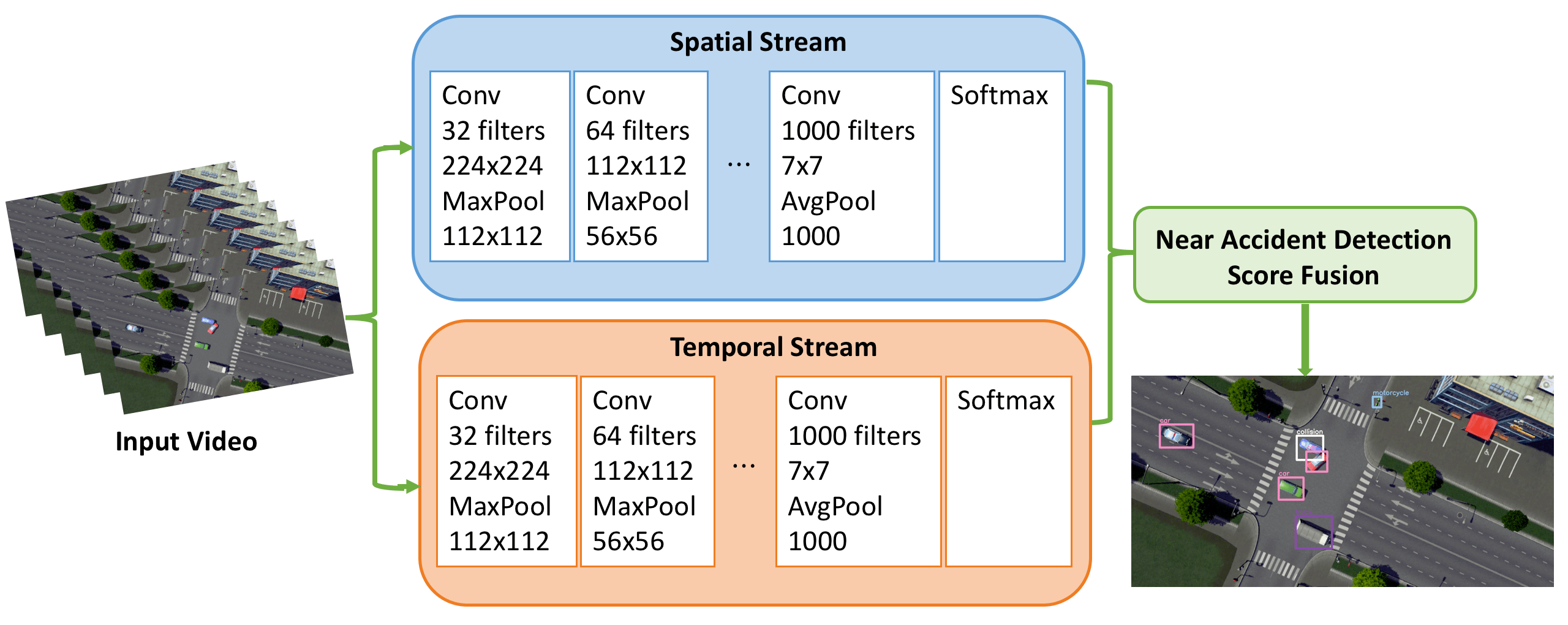
Figure 1. Two-stream architecture for near accident detection.

3. Two-Stream architecture for Near Accident Detection

We present our vision-based two-stream architecture for real-time near accident detection based on real-time object detection and multiple object tracking. The goal of near accident detection is to detect likely collision scenarios across video frames and report these near accident records. As videos can be decomposed into spatial and temporal components. We divide our framework into a two-stream architecture as shown in Fig 1. The spatial part consists of individual frame appearance information about scenes and objects in the video. The temporal part contains motion information for moving objects. For spatial stream convolutional neural network, we utilized a standard convolutional network of a state-of-the-art object detection method (Redmon et al., 2016) to detect individual vehicles and likely near accident regions at the single frame level. The temporal stream network is leveraging object candidates from object detection CNNs and integrates their appearance information with a fast multiple object tracking method to extract motion features and compute trajectories. When two trajectories of individual objects start intersecting or become closer than a certain threshold, we’ll label the region covering two objects as high probability near accident regions. Finally, we take average near accident probability of spatial stream network and temporal stream network and report the near accident record.

3.1. Preliminaries

Convolutional Neural Networks: Convolutional Neural Networks (CNNs) have a strong capability of representing objects and helps to boost the performance of numerous vision tasks, comparing to traditional heuristic features (Dalal and Triggs, 2005). A Convolutional Neural Networks (CNN) is a a class of deep neural networks which is widely applied for visual imagery analysis in computer vision. A standard CNN usually consists of an input and an output layer, as well as multiple hidden layers (convolutional layers, pooling layers, fully connected layers and normalization layers) as shown in Figure 2. The input to a convolutional layer is an original image $\bm{X}$. We denote the feature map of $i$-th convolutional layer as $\bm{H}_{i}$ and $\bm{H}_{0}=\bm{X}$. Then $\bm{H}_{i}$ can be described as

(2) $${\bm{H}_{i}}=f\left({{\bm{H}_{i-1}}\otimes{\bm{W}_{i}}+{\bm{b}_{i}}}\right)$$

where $\bm{W}_{i}$ is the weight for $i$-th convolutional kernel, and $\otimes$ is the convolution operation of the kernel and $i-1$-th image or feature map. Output of convolution operation are summed with a bias $\bm{b}_{i}$. Then the feature map for $i$-th layer can be computed by applying a nonlinear activation function to it. Take an example of using a $32\times 32$ RGB image with a simple ConvNet for CIFAR-10 classification (Krizhevsky and Hinton, 2009).

• Input layer: the original image with raw pixel values as width is 32, height is 32, and color channels (R,G,B) is 3.

• Convolutional layer: compute output of neurons which are connected to local regions in the image through activation functions. If we use 12 filters, we have result in volume such as $[32\times 32\times 12]$.

• Pooling layer: perform a downsampling operation, resulting in volume such as $[16\times 16\times 12]$.

• Fully connected layer: compute the class scores, resulting in volume of size $[1\times 1\times 10]$, where these 10 numbers are corresponding to 10 class score.

In this way, CNNs transform the original image into multiple high-level feature representations layer by layer and compute the final final class scores.

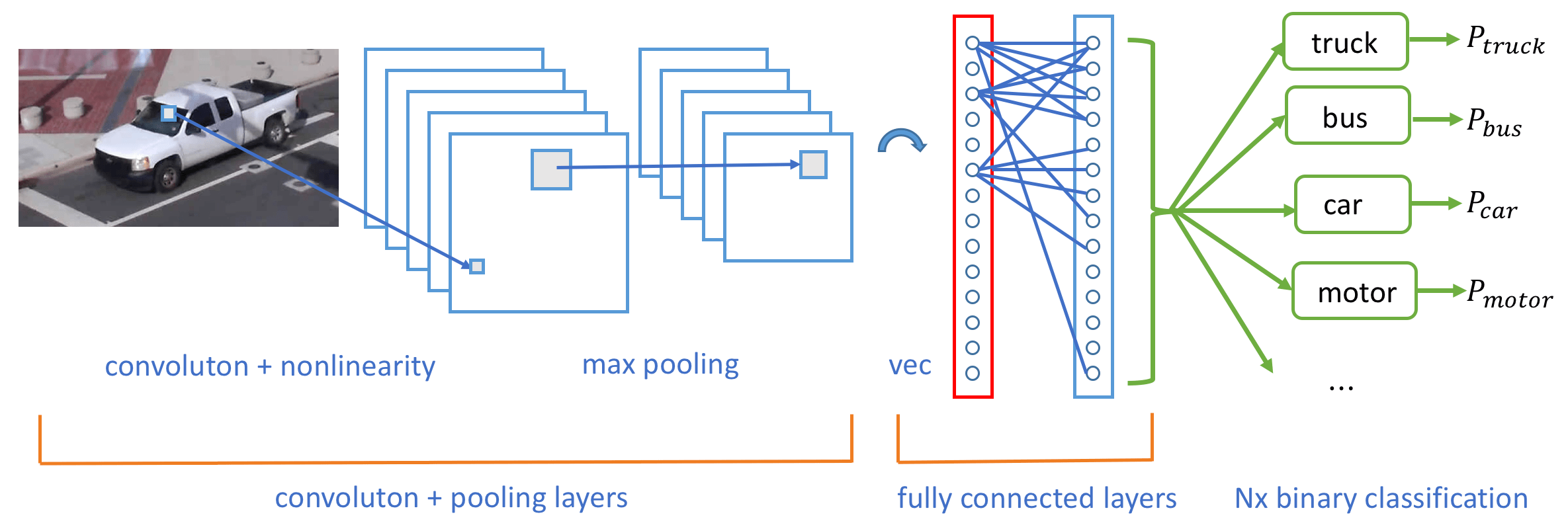
Figure 2. Architecture of Convolutional Neural Networks for image classification.

3.2. Spatial stream network

In our framework, each stream is implemented using a deep convolutional neural network. Near accident scores are combined by the averaging score. Since our spatial stream ConvNet is essentially an object detection architecture, we build it upon the recent advances in object detection with YOLO detector (Redmon et al., 2016), and pre-train the network from scratch on our dataset containing multi-scale drone, fisheye and simulation videos. As most of our videos contain traffic scenes with vehicles and traffic movement in top-down view, we specify different vehicle classes such as motorcycle, car, bus, and truck as object classes for training the detector. Additionally, near accident or collision can be detected from single still frame either from the beginning of a video or stopped vehicles associated in an accident after collision. Therefore, we train our detector to localize these likely near accident scenarios. Since the static appearance is a useful cue, the spatial stream network effectively performs object detection by operating on individual video frames.

3.2.1. YOLO object detection

You Only Look Once (YOLO) (Redmon et al., 2016) is a state-of-the-art, real-time object detection system. This end-to-end deep learning approach does not need region proposals and is much different from the region based algorithms. The pipeline of YOLO (Redmon et al., 2016) is pretty straightforward: YOLO (Redmon et al., 2016) passes the whole image through the neural network only once where the title comes from (You Only Look Once) and returns bounding boxes and class probabilities for predictions. Figure 3 demonstrates the detection model and system of YOLO (Redmon et al., 2016). In YOLO (Redmon et al., 2016), it regards object detection as an end-to-end regression problem and uses a single convolutional network predicts the bounding boxes and the class probabilities for these boxes. It first takes the image and split it into an $S\times S$ grid, within each of the grid we take $m$ bounding boxes. For each grid cell,

• it predicts B boundary boxes and each box has one box confidence score

• it detects one object only regardless of the number of boxes B

• it predicts C conditional class probabilities (one per class for the likeliness of the object class)

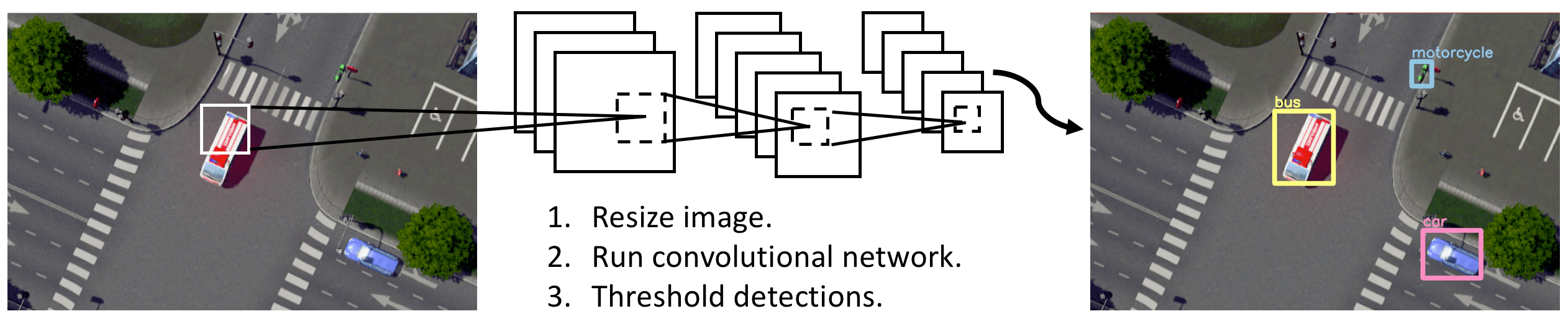
Figure 3. The YOLO Detection System (Redmon et al., 2016). It (1) resizes the input image to $448\times 448$, (2) runs a single convolutional network on the image, and (3) thresholds the resulting detections by the model’s confidence.

For each of the bounding box, the convolutional neural network (CNN) outputs a class probability and offset values for the bounding box. Then it selects bounding boxes which have the class probability above a threshold value and uses them to locate the object within the image. In detail, each boundary box contains 5 elements: $(x,y,w,h)$ and a box confidence. The $(x,y)$ are coordinates which represent the center of the box relative to the bounds of the grid cell. The $(w,h)$ are width and height. These elements are normalized as $x$, $y$, $w$ and $h$ are all between 0 and 1. The confidence prediction represents the intersection over union (IoU) between the predicted box and any ground truth box which reflects how likely the box contains an object (objectness) and how accurate is the boundary box. The mathematical definitions of those scoring and probability terms are:

box confidence score $\equiv P_{r}(object)\cdot IoU$

conditional class probability $\equiv P_{r}(class_{i}|object)$

class confidence score $\equiv P_{r}(class_{i})\cdot IoU$

class confidence score $=$ box confidence score $\times$ conditional class probability

where $\equiv P_{r}(object)$ is the probability the box contains an object. $IoU$ is the IoU between the predicted box and the ground truth. $\equiv P_{r}(class_{i})$ is the probability the object belongs to $class_{i}$. $\equiv P_{r}(class_{i}|object)$ is the probability the object belongs to $class_{i}$ given an object is presence. The network architecture of YOLO (Redmon et al., 2016) simply contains 24 convolutional layers followed by two fully connected layers, reminiscent of AlexNet and even earlier convolutional architectures. Some convolution layers use $1\times 1$ reduction layers alternatively to reduce the depth of the features maps. For the last convolution layer, it outputs a tensor with shape $(7,7,1024)$ which is flattened. YOLO (Redmon et al., 2016) performs a linear regression using two fully connected layers to make boundary box predictions and to make a final prediction using threshold of box confidence scores. The final loss adds localization, confidence and classification losses together.

Type	Filters	Size/Stride	Output
Convolutional	32	$3\times 3$	$224\times 224$
Maxpool		$2\times 2/2$	$112\times 112$
Convolutional	64	$3\times 3$	$112\times 112$
Maxpool		$2\times 2/2$	$56\times 56$
Convolutional	128	$3\times 3$	$56\times 56$
Convolutional	64	$1\times 1$	$56\times 56$
Convolutional	128	$3\times 3$	$56\times 56$
Maxpool		$2\times 2/2$	$28\times 28$
Convolutional	256	$3\times 3$	$28\times 28$
Convolutional	128	$1\times 1$	$28\times 28$
Convolutional	256	$3\times 3$	$28\times 28$
Maxpool		$2\times 2/2$	$14\times 14$
Convolutional	512	$3\times 3$	$14\times 14$
Convolutional	256	$1\times 1$	$14\times 14$
Convolutional	512	$3\times 3$	$14\times 14$
Convolutional	256	$1\times 1$	$14\times 14$
Convolutional	512	$3\times 3$	$14\times 14$
Maxpool		$2\times 2/2$	$7\times 7$
Convolutional	1024	$3\times 3$	$7\times 7$
Convolutional	512	$1\times 1$	$7\times 7$
Convolutional	1024	$3\times 3$	$7\times 7$
Convolutional	512	$1\times 1$	$7\times 7$
Convolutional	1024	$3\times 3$	$7\times 7$
Convolutional	1000	$1\times 1$	$7\times 7$
Avgpool		Global	$1000$
Softmax

Table 1. Darknet-19 (Redmon and Farhadi, 2017).

(3) $$\lambda_{\textbf{coord}}\sum_{i=0}^{S^{2}}\sum_{j=0}^{B}{\mathbbm{1}}_{ij}^{\text{obj}}\left[\left(x_{i}-\hat{x}_{i}\right)^{2}+\left(y_{i}-\hat{y}_{i}\right)^{2}\right]+\lambda_{\textbf{coord}}\sum_{i=0}^{S^{2}}\sum_{j=0}^{B}{\mathbbm{1}}_{ij}^{\text{obj}}\left[\left(\sqrt{w_{i}}-\sqrt{\hat{w}_{i}}\right)^{2}+\left(\sqrt{h_{i}}-\sqrt{\hat{h}_{i}}\right)^{2}\right]\\ +\sum_{i=0}^{S^{2}}\sum_{j=0}^{B}{\mathbbm{1}}_{ij}^{\text{obj}}\left(C_{i}-\hat{C}_{i}\right)^{2}+\lambda_{\textrm{noobj}}\sum_{i=0}^{S^{2}}\sum_{j=0}^{B}{\mathbbm{1}}_{ij}^{\text{noobj}}\left(C_{i}-\hat{C}_{i}\right)^{2}+\sum_{i=0}^{S^{2}}{\mathbbm{1}}_{i}^{\text{obj}}\sum_{c\in\textrm{classes}}\left(p_{i}(c)-\hat{p}_{i}(c)\right)^{2}$$

where $\mathbbm{1}_{i}^{\text{obj}}$ denotes if object appears in cell $i$ and $\mathbbm{1}_{ij}^{\text{obj}}$ denotes that the $j$th bounding box predictor in cell $i$ is “responsible” for that prediction. YOLO (Redmon et al., 2016) is orders of magnitude faster (45 frames per second) than other object detection approaches which means it can process streaming video in realtime and achieves more than twice the mean average precision of other real-time systems. For the implementation, we leverage the extension of YOLO (Redmon et al., 2016), Darknet-19, a classification model that used as the base of YOLOv2 (Redmon and Farhadi, 2017). The full network description of it is shown in Table 1. Darknet-19 (Redmon and Farhadi, 2017) has 19 convolutional layers and 5 maxpooling layers and it uses batch normalization to stabilize training, speed up convergence, and regularize the model (Ioffe and Szegedy, 2015).

3.3. Temporal stream network

The spatial stream network is not able to extract motion features and compute trajectories due to single-frame inputs. To leverage these useful information, we present our temporal stream network, a ConvNet model which performs a tracking-by-detection multiple object tracking algorithm (Bewley et al., 2016; Wojke et al., 2017) with data association metric combining deep appearance features. The inputs are identical to the spatial stream network using the original video. Detected object candidates (only vehicle classes) are used to for tracking handling, state estimation, and frame-by-frame data association using SORT (Bewley et al., 2016) and DeepSORT (Wojke et al., 2017), the real-time multiple object tracking methods. The multiple object tracking models each state of objects and describes the motion of objects across video frames. With tracking, we obtain results by stacking trajectories of moving objects between several consecutive frames which are useful cues for near accident detection.

3.3.1. SORT

Simple Online Realtime Tracking (SORT) (Bewley et al., 2016) is a simple, popular and fast Multiple Object Tracking (MOT) algorithm. The core idea is to perform a Kalman filtering (Kalman, 1960) in image space and do frame-by-frame data association using the Hungarian methods (Kuhn, 1955) with an association metric that measures bounding box overlap. Despite only using a rudimentary combination of the Kalman Filter (Kalman, 1960) and Hungarian algorithm (Kuhn, 1955) for the tracking components, SORT (Bewley et al., 2016) achieves an accuracy comparable to state-of-the-art online trackers. Moreover, due to the simplicity of it, SORT (Bewley et al., 2016) can updates at a rate of 260 Hz on single machine which is over 20x faster than other state-of-the-art trackers.

Estimation Model. The state of each target is modelled as:

(4) $$\mathbf{x}=[u,v,s,r,\dot{u},\dot{v},\dot{s}]^{T},$$

where $u$ and $v$ represent the horizontal and vertical pixel location of the centre of the target, while the scale $s$ and $r$ represent the scale (area) and the aspect ratio (usually considered to be constant) of the target’s bounding box respectively. When a detection is associated to a target, it updates the target state using the detected bounding box where the velocity components are solved optimally via a Kalman filter framework (Kalman, 1960). If no detection is associated to the target, its state is simply predicted without correction using the linear velocity model.

Data Association. In order to assign detections to existing targets, each target’s bounding box geometry is estimated by predicting its new location in the current frame. The assignment cost matrix is defined as the IoU distance between each detection and all predicted bounding boxes from the existing targets. Then the assignment problem is solved optimally using the Hungarian algorithm (Kuhn, 1955). Additionally, a minimum IoU is imposed to reject assignments where the detection to target overlap is less than $IoU_{min}$. The IoU distances of the bounding boxes are found so as to handle short term occlusion caused by passing targets.

Creation and Deletion of Track Identities. When new objects enter or old objects vanish in video frames, unique identities for objects need to be created or destroyed accordingly. For creating trackers, we consider any detection with an overlap less than $IoU_{min}$ to signify the existence of an untracked object. Then the new tracker undergoes a probationary period where the target needs to be associated with detections to accumulate enough evidence in order to prevent tracking of false positives. Tracks could be terminated if they are not detected for $T_{Lost}$ frames to prevent an unbounded growth in the number of trackers and localization errors caused by predictions over long durations without corrections from the detector.

3.3.2. DeepSORT

DeepSORT (Wojke et al., 2017) is an extension of SORT (Bewley et al., 2016) which integrates appearance information through a pre-trained association metric to improve the performance of SORT (Bewley et al., 2016). It adopts a conventional single hypothesis tracking methodology with recursive Kalman filtering (Kalman, 1960) and frame-by-frame data association. DeepSORT (Wojke et al., 2017) helps to solve a large number of identities switching problem in SORT (Bewley et al., 2016) and it can track objects through longer periods of occlusions. During online application, it establishs measurement-to-track associations using nearest neighbor queries in visual appearance space.

Track Handling and State Estimation. The track handling and state estimation using Kalman filtering (Kalman, 1960) is mostly identical to the SORT (Bewley et al., 2016). The tracking scenario is defined using eight dimensional state space $(u,v,\gamma,h,\dot{x},\dot{y},\dot{\gamma},\dot{h})$ that contains the bounding box center position $(u,v)$, aspect ratio $\gamma$, height $h$, and their respective velocities in image coordinates. It uses a standard Kalman filter (Kalman, 1960) with a constant velocity motion and linear observation model, where it takes the bounding coordinates $(u,v,\gamma,h)$ as direct observations of the object state.

Data Association. To solve the frame-by-frame association problem between the predicted Kalman states and the newly arrived measurements, it uses the Hungarian algorithm (Kuhn, 1955). In formulation, it integrates both motion and appearance information through combination of two appropriate metrics. For motion information, the (squared) Mahalanobis distance between predicted Kalman states and newly arrived measurements is utilized:

(5) $$d^{(1)}(i,j)=(\bm{d}_{j}-\bm{y}_{i})^{\bm{T}}(\bm{S}_{i})^{-1}(\bm{d}_{j}-\bm{y}_{i})$$

where the projection of the $i$-th track distribution into measurement space is  $(\bm{y}_{i},\bm{S}_{i})$ and the $j$-th bounding box detection is $\bm{d}_{j}$. The second metric measures the smallest cosine distance between the $i$-th track and $j$-th detection in appearance space:

(6) $$d^{(2)}(i,j)=\min\left\{1-{\bm{r}_{j}}^{T}\bm{r}^{(i)}_{k}|\bm{r}^{(i)}_{k}\in\mathcal{R}_{i}\right\}$$

Then this association problem is built with combination of both metrics using a weighted sum where the influence of each metric on combined association cost can be controlled through hyperparameter $\lambda$.

(7) $$c_{i,j}=\lambda\,d^{(1)}(i,j)+(1-\lambda)d^{(2)}(i,j)$$

Matching Cascade. Rather than solving measurement-to-track associations in a global way, it adopts a matching cascade introduced in (Wojke et al., 2017) to solve a series of subproblems. In some situation, when occlusion happens to a object for a longer period of time, the subsequent Kalman filter (Kalman, 1960) predictions would increase the uncertainty associated with the object location. In consequent, probability mass spreads out in state space and the observation likelihood becomes less peaked. Intuitively, the association metric should account for this spread of probability mass by increasing the measurement-to-track distance. Therefore, the matching cascade strategy gives priority to more frequently seen objects to encode the notion of probability spread in the association likelihood.

3.4. Near Accident Detection

When utilizing the multiple object tracking algorithm, we compute the center of each object in several consecutive frames to form stacking trajectories as our motion representation. These stacking trajectories can provide accumulated information through image frames, including the number of objects, their motion history and timing of their interactions such as near accident. We stack the trajectories of all object by every $L$ consecutive frames as illustrated in Figure 4 where $\mathbf{p}_{t}^{i}$ denotes the center position of the $i$-th object in the $t$-th frame. $\mathbf{P}_{t}=(\mathbf{p}_{t}^{1},\mathbf{p}_{t}^{2},...,\mathbf{p}_{t}^{M_{t}})$ denotes trajectories of all the $M_{t}$ objects in the $t$-th frame. $\mathbf{P}_{1:t}=\{\mathbf{P}_{1},\mathbf{P}_{2},...,\mathbf{P}_{t}\}$ denotes all the sequential trajectories of all the objects from the first frame to the $t$-th frame. As we only exam every $L$ consecutive frames, the stacking trajectories are sequentially as

(8) $$\mathbf{P}_{1:L}=\{\mathbf{P}_{1},\mathbf{P}_{2},...,\mathbf{P}_{L}\},\mathbf{P}_{L+1:2L}=\{\mathbf{P}_{L+1},\mathbf{P}_{L+2},...,\mathbf{P}_{2L}\},\cdots$$

$\mathbf{O}_{t}=(\mathbf{o}_{t}^{1},\mathbf{o}_{t}^{2},...,\mathbf{o}_{t}^{M_{t}})$ denotes the collected observations for all the $M_{t}$ objects in the $t$-th frame. $\mathbf{O}_{1:t}=\{\mathbf{O}_{1},\mathbf{O}_{2},...,\mathbf{O}_{t}\}$ denotes all the collected sequential observations of all the objects from the first frame to the $t$-th frame. We use a simple detection algorithm which finds collisions between simplified forms of the objects, using the center of bounding boxes.

Our algorithm is depicted in Algorithm 1. Once the collision is detected, we set the region covering collision associated objects to be a new bounding box with class probability of near accident to be 1. By averaging the near accident probability of output from spatial stream network and temporal stream network, we are able to compute the final outputs of near accident detection.

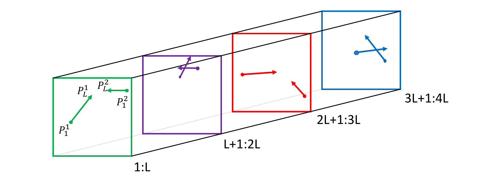
Figure 4. The stacking trajectories extracted from tracking. Consecutive frames and the corresponding displacement vectors are shown with the same colour.

Input: current frame $t_{current}$, collision state list $Collision$

Output: collision state list $Collision$

for $t_{L}\leftarrow t_{previous}$ to $t_{current}$ in steps of $L$ frames do

       for each pair of object trajectory ($\mathbf{p}_{:t_{L}}^{1}$, $\mathbf{p}_{:t_{L}}^{2})$ do

             if ($\mathbf{p}_{:t_{L}}^{1}$ intersects $\mathbf{p}_{:t_{L}}^{2}$ as of $t_{L}$) then

                  add $\mathbf{o}_{1}$, $\mathbf{o}_{2}$ to $Collision$

             end if

            

       end for

      if ($Collisions$) then

            $t_{previous}\leftarrow t_{L}$; return TRUE

       end if

      

end for

$t_{previous}\leftarrow t_{d}$; return FALSE

ALGORITHM 1 Collision Detection

4. Experiments

In this section, we first introduce our novel traffic near accident dataset (TNAD) and describe the preprocessing, implementation detail and experiments settings. Finally, we present qualitative and quantitative evaluation in terms of the performance of object detection, multiple object tracking, and near accident detection, and comparison between other methods and our framework.

4.1. Traffic Near Accident Dataset (TNAD)

As we mentioned in Section 2, there is no such a comprehensive traffic near accident dataset containing top-down views videos such as drone/Unmanned Aerial Vehicles (UAVs) videos, or omnidirectional camera videos for traffic analysis. Therefore, we have built our own dataset, traffic near accident dataset (TAND) which is depicted in Figure 5. Intersections tend to experience more and severe near accident due to factors such as angles and turning collisions. Traffic Near Accident Dataset (TNAD) containes 3 types of video data of traffic intersections that could be utilized for not only near accident detection but also other traffic surveillance tasks including turn movement counting.

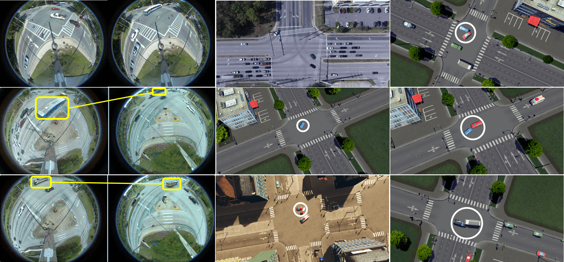
Figure 5. Samples of Traffic Near Accident Dataset (TNAD). Our dataset consists of a large number of diverse intersection surveillance videos and different near accident (cars and motorcycles). Yellow rectangles and lines represent the same object in multi-camera video. White circles represent the near accident regions.

The first type is drone video that monitoring an intersection with top-down view. The second type of intersection videos is real traffic videos acquired by omnidirectional fisheye cameras that monitoring small or large intersections. It is widely used in transportation surveillance. These video data can be directly used as input for our vision-intelligent framework, and also pre-processing of fisheye correction can be applied to them for better surveillance performance. The third type of video is video data simulated by game engine for the purpose to train and test with more near accident samples. The traffic near accident dataset (TAND) consists of 106 videos with total duration over 75 minutes with frame rates between 20 fps to 50 fps. The drone video and fisheye surveillance videos are recorded in Gainesville, Florida at several different intersections. Our videos are challenging than videos in other datasets due to the following reasons:

• Diverse intersection scene and camera perspectives: The intersections in drone video, fisheye surveillance video, and simulation video are much different. Additionally, the fisheye surveillance video has distortion and fusion technique is needed for multi-camera fisheye videos.

• Crowded intersection and small object: The number of moving cars and motorbikes per frame are large and these objects are relatively smaller than normal traffic video.

• Diverse accidents: Accidents involving cars and motorbikes are all included in our dataset.

• Diverse Lighting condition: Different lighting conditions such as daylight and sunset are included in our dataset.

We manually annotate the spatial location and temporal locations of near accidents and the still/moving objects with different vehicle class in each video. 32 videos with sparse sampling frames (only 20% frames of these 32 videos are used for supervision) are used only for training the object detector. The remaining 74 videos are used for testing.

4.2. Fisheye and multi-camera video

The fisheye surveillance videos are recorded from real traffic data in Gainesville. We have collected 29 single-camera fisheye surveillance videos and 19 multi-camera fisheye surveillance videos monitoring a large intersection. We conduct two experiments, one directly using these raw videos as input for our system and another is first to do preprocessing for correcting fisheye distortion on video level and feed them into our system. As the original survellance video has many visual distortions especially near the circular boundaries of cameras, our system performs better on these after preprocessing videos. Therefore we keep the distortion correction preprocessing in the experiments for fisheye videos.

For large intersection, two fisheye cameras placed at opposite directions are used for surveillance and each of them mostly shows half of roads and real traffic for the large intersection. In this paper, we do not investigate the real stitching problem (we’ll leave it for further work). First, we do fisheye distortion correction and combine the two video with similar points. Then we apply a simple object level stitching methods by assigning the object identity for the same objects across the left and right video using similar features and appearing/vanishing positions.

4.3. Model Training

The layer configuration of our spatial and temporal convolutional neural networks (based on Darknet-19 (Wojke et al., 2017)) is schematically shown in Table 1. We adopt the Darknet-19 (Wojke et al., 2017) for classification and detection with deepSORT using data association metric combining deep appearance feature. We implement our framework on Tensorflow and do multi-scale training and testing with a single GPU (Nvidia Titan X Pascal). Training a single spatial convolutional network takes 1 day on our system with 1 Nvidia Titan X Pascal card. For classification and detection training, we use the same training strategy as YOLO9000 (Wojke et al., 2017). We train the network on our TNAD dataset with 4 class of vehicle (motorcycle, bus, car, and truck) for 160 epochs using stochastic gradient descent with a starting learning rate of 0.1 for classification, and $10^{-3}$ for detection (dividing it by 10 at 60 and 90 epochs.), weight decay of 0.0005 and momentum of 0.9 using the Darknet neural network framework (Wojke et al., 2017).

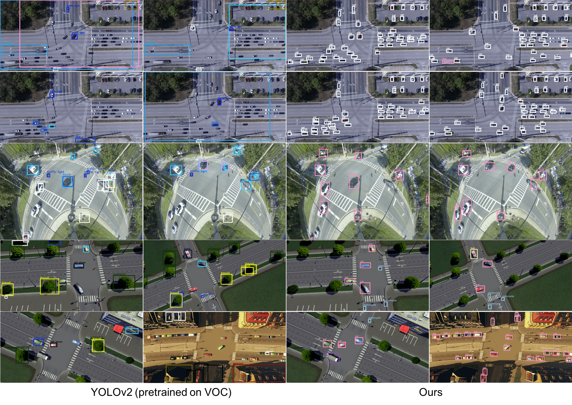
Figure 6. Sample results of object detection on TNAD dataset. Left and middle left: results of directly using YOLOv2 (Redmon and Farhadi, 2017) detector pretrained on generic objects (VOC dataset) (Everingham et al., 2015b). Middle right and right: results of our spatial network with multi-scale training based on YOLOv2 (Redmon and Farhadi, 2017).

Figure 7. Tracking and trajectory comparison with Urban Tracker (Jodoin et al., 2014) and TrafficIntelligence (Jackson et al., 2013) on drone videos of TNAD dataset.Left: results of Urban Tracker (Jodoin et al., 2014)(BSG with Multilayer and Lobster Model). Middle: results of TrafficIntelligence (Jackson et al., 2013). Right: results of our spatial network.

Figure 8. Sample results of tracking, trajectory and near accident detection of our two-stream Convolutional Networks on simulation videos of TNAD dataset.Left: tracking results based on DeepSORT (Wojke et al., 2017). Middle: trajectory results of our spatial network.  (Jackson et al., 2013).Right: near accident detection results of our two-stream Convolutional Networks.

Table 2. Frame level near accident detection results

Video ID	near Accident (pos/neg)	# of frame for positive Near accident (groundtruth)/total frame	# of frame for correct localization (IoU ¿= 0.6)	# of frame for incorent localization (IoU¡0.6)
1	pos	12/245	12	0
2	neg	0/259	0	0
3	neg	0/266	0	0
4	pos	16/267	13	0
5	pos	6/246	4	0
6	pos	4/243	4	0
7	neg	0/286	0	0
8	pos	2/298	0	0
9	pos	27/351	23	6
10	neg	0/301	0	0
11	neg	0/294	0	0
12	pos	6/350	6	6
13	neg	0/263	0	0
14	pos	5/260	5	0
15	pos	4/326	4	0
16	neg	0/350	0	0
17	neg	0/318	0	1
18	pos	10/340	8	0
19	pos	6/276	0	0
20	pos	8/428	4	0
21	neg	0/259	0	0
22	pos	10/631	8	0
23	pos	35/587	30	2
24	neg	0/780	0	0
25	neg	0/813	0	0
26	neg	0/765	0	0
27	pos	8/616	8	0
28	pos	10/243	10	1
29	pos	6/259	6	0
30	pos	17/272	15	3

4.4. Qualitative results

We present some example experimental results of object detection, multiple object tracking and near accident detection on our traffic near accident dataset (TNAD) for drone videos, fisheye videos, and simulation videos. For object detection (Figure 6), we present some detection results of directly using YOLO detector (Redmon and Farhadi, 2017) trained on generic objects (VOC dataset) (Everingham et al., 2015b) and results of our spatial network with multi-scale training based on YOLOv2 (Redmon and Farhadi, 2017). For multiple object tracking (Figure 7), we present comparison of our temporal network based on DeepSORT (Wojke et al., 2017) with Urban Tracker (Jodoin et al., 2014) and TrafficIntelligence (Jackson et al., 2013). For near accident detection (Figure 8), we present near accident detection results along with tracking and trajectories using our two-stream Convolutional Networks method. The object detection results shows that, with multi-scale training on TNAD dataset, the performance of the detector significant improves. It can perform well vehicle detection on top-down view surveillance videos even for small objects. In addition, we can achieve fast detection rate at 20 to 30 frame per second. Overall, this demonstrates the effectiveness of our spatial neural network. For the tracking part, since we use a tracking-by-detection paradigm, our methods can handle still objects and measure their state where Urban Tracker (Jodoin et al., 2014) and TrafficIntelligence (Jackson et al., 2013) can only handle tracking for moving objects. On the other hand, Urban Tracker (Jodoin et al., 2014) and TrafficIntelligence (Jackson et al., 2013) can compute dense trajectories of moving objects with good accuracy but they have slower tracking speed around 1 frame per second. For accident detection, our two-stream Convolutional Networks are able to do spatial localization and temporal localization for diverse accidents regions involving cars and motorcycles. The three sub-tasks (object detection, multiple object tracking and near accident detection) can always achieve real-time performance at high frame rate, 20 to 30 frame per second according to the frame resolution (e.g. 28 fps for 960$\times$480 image frame). Overall, the qualitative results demonstrate the effectiveness of our spatial neural network and temporal network respectively.

Table 3. Quantitative evaluation.

Benchmark Result		Predicted
		Negative	Positive
Actual	Negative	11081	19
	Positive	32	160

4.5. Quantitative results

Since our frame has three tasks and our dataset are much different than other object detection dataset, tracking dataset and near accident dataset such as dashcam accident dataset (Chan et al., 2016), it is difficult to compare individual quantitative performance for all three tasks with other methods. One of our motivation is to propose a vision-based solution for Intelligent Transportation System, we focus more on near accident detection and present quantitative analysis of our two-stream Convolutional Networks. The simulation videos are for the purpose to train and test with more near accident samples and we have 57 simulation videos with a total over 51,123 video frames. We sparsely sample only 1087 frames from them for whole training processing. We present the analysis of near accident detection for 30 testing videos (18 has positive near accident, 12 has negative near accident). Table 2 shows frame level near accident detection performance on 30 testing simulation videos. The performance of precision, recall and F-measure are presented in Table 3. If a frame contains a near accident scenario and we can successfully localize it with Intersection of union (IoU) is large or equal than 0.6, this is a True Positive (TP). If we cannot localize it or localize it with Intersection of Union (IoU) is less than 0.6, this is a False Negative (FN). If a frame has no near accident scenario but we detect a near accident region, this is a False Positive (FP). Otherwise, this is a True Negative (TN). We compute the $\text{precision}=\frac{\text{TP}}{\text{TP + FP}}$, $\text{recall}=\frac{\text{TP}}{\text{TP + FN}}$, and F-measure $\text{F-measure}=\frac{2\times\text{precision}\times\text{recall}}{\text{precision + recall}}=\frac{\text{2TP}}{\text{2TP + FP + FN}}$. Our precision is about 0.894, recall is about 0.8333 and F1 score is about 0.863. The three sub-tasks (object detection, multiple object tracking and near accident detection) can always achieve real-time performance at high frame rate, 20 30 frame per second according to the frame resolution (e.g. 28 fps for 960$\times$480 image frame). In conclusion, we have demonstrated that our two-stream Convolutional Networks have an overall competitive performance for near accident detection on our TNAD dataset.

5. Conclusion

We have proposed a two-stream Convolutional Network architecture that performs real-time detection, tracking, and near accident detection of road users in traffic video data. The two-stream Convolutional Networks consist of a spatial stream network to detect individual vehicles and likely near accident regions at the single frame level, by capturing appearance features with a state-of-the-art object detection method. The temporal stream network leverages motion features of detected candidates to perform multiple object Tracking and generate individual trajectories of each tracking target. We detect near accident by incorporating appearance features and motion features to compute probabilities of near accident candidate regions. We have present a challenging Traffic Near Accident dataset (TNAD), which contains different types of traffic interaction videos that can be used for several vision-based traffic analysis tasks. On the TNAD dataset, experiments have demonstrated the advantage of our framework with an overall competitive qualitative and quantitative performance at high frame rates. The future direction of the work is the image stitching mehtods for our proposed multi-camera fisheye videos.

- (1)
- Angel et al. (2002) Alejandro Angel, Mark Hickman, Pitu Mirchandani, and Dmesh Chandnani. 2002. Methods of traffic data collection, using aerial video. In Intelligent Transportation Systems, 2002. Proceedings. The IEEE 5th International Conference on. IEEE, 31–36.
- Bewley et al. (2016) Alex Bewley, Zongyuan Ge, Lionel Ott, Fabio Ramos, and Ben Upcroft. 2016. Simple online and realtime tracking. In Image Processing (ICIP), 2016 IEEE International Conference on. IEEE, 3464–3468.
- Bhonsle et al. (2000) Shailendra Bhonsle, Mohan Trivedi, and Amarnath Gupta. 2000. Database-centered architecture for traffic incident detection, management, and analysis. In Intelligent Transportation Systems, 2000. Proceedings. 2000 IEEE. IEEE, 149–154.
- Buch et al. (2011) Norbert Buch, Sergio A Velastin, and James Orwell. 2011. A review of computer vision techniques for the analysis of urban traffic. IEEE Transactions on Intelligent Transportation Systems 12, 3 (2011), 920–939.
- Chan et al. (2016) Fu-Hsiang Chan, Yu-Ting Chen, Yu Xiang, and Min Sun. 2016. Anticipating accidents in dashcam videos. In Asian Conference on Computer Vision. Springer, 136–153.
- Chen et al. (2010) Lairong Chen, Yuan Cao, and Ronghua Ji. 2010. Automatic incident detection algorithm based on support vector machine. In Natural Computation (ICNC), 2010 Sixth International Conference on, Vol. 2. IEEE, 864–866.
- Chen et al. (2016) Yu Chen, Yuanlong Yu, and Ting Li. 2016. A vision based traffic accident detection method using extreme learning machine. In Advanced Robotics and Mechatronics (ICARM), International Conference on. IEEE, 567–572.
- Coifman et al. (1998) Benjamin Coifman, David Beymer, Philip McLauchlan, and Jitendra Malik. 1998. A real-time computer vision system for vehicle tracking and traffic surveillance. Transportation Research Part C: Emerging Technologies 6, 4 (1998), 271–288.
- Dalal and Triggs (2005) Navneet Dalal and Bill Triggs. 2005. Histograms of oriented gradients for human detection. In Computer Vision and Pattern Recognition, 2005. CVPR 2005. IEEE Computer Society Conference on, Vol. 1. IEEE, 886–893.
- Everingham et al. (2015a) Mark Everingham, SM Ali Eslami, Luc Van Gool, Christopher KI Williams, John Winn, and Andrew Zisserman. 2015a. The pascal visual object classes challenge: A retrospective. International journal of computer vision 111, 1 (2015), 98–136.
- Everingham et al. (2015b) M. Everingham, S. M. A. Eslami, L. Van Gool, C. K. I. Williams, J. Winn, and A. Zisserman. 2015b. The Pascal Visual Object Classes Challenge: A Retrospective. International Journal of Computer Vision 111, 1 (Jan. 2015), 98–136.
- Everingham et al. (2010) Mark Everingham, Luc Van Gool, Christopher KI Williams, John Winn, and Andrew Zisserman. 2010. The pascal visual object classes (voc) challenge. International journal of computer vision 88, 2 (2010), 303–338.
- Gardner and Lawton (1996) Warren F Gardner and Daryl T Lawton. 1996. Interactive model-based vehicle tracking. IEEE Transactions on Pattern Analysis and Machine Intelligence 18, 11 (1996), 1115–1121.
- Ghosh-Dastidar and Adeli (2003) Samanwoy Ghosh-Dastidar and Hojjat Adeli. 2003. Wavelet-clustering-neural network model for freeway incident detection. Computer-Aided Civil and Infrastructure Engineering 18, 5 (2003), 325–338.
- Girshick (2015) Ross Girshick. 2015. Fast r-cnn. In Proceedings of the IEEE international conference on computer vision. 1440–1448.
- Girshick et al. (2014) Ross Girshick, Jeff Donahue, Trevor Darrell, and Jitendra Malik. 2014. Rich feature hierarchies for accurate object detection and semantic segmentation. In Proceedings of the IEEE conference on computer vision and pattern recognition. 580–587.
- Girshick et al. (2016) Ross Girshick, Jeff Donahue, Trevor Darrell, and Jitendra Malik. 2016. Region-based convolutional networks for accurate object detection and segmentation. IEEE transactions on pattern analysis and machine intelligence 38, 1 (2016), 142–158.
- He et al. (2017) Pan He, Weilin Huang, Tong He, Qile Zhu, Yu Qiao, and Xiaolin Li. 2017. Single Shot Text Detector With Regional Attention. In Proceedings of the IEEE International Conference on Computer Vision. 3047–3055.
- Hearst et al. (1998) Marti A. Hearst, Susan T Dumais, Edgar Osuna, John Platt, and Bernhard Scholkopf. 1998. Support vector machines. IEEE Intelligent Systems and their applications 13, 4 (1998), 18–28.
- Hermes et al. (2009) Christoph Hermes, Christian Wohler, Konrad Schenk, and Franz Kummert. 2009. Long-term vehicle motion prediction. In Intelligent Vehicles Symposium, 2009 IEEE. IEEE, 652–657.
- Hommes et al. (2011) Stefan Hommes, Radu State, Andreas Zinnen, and Thomas Engel. 2011. Detection of abnormal behaviour in a surveillance environment using control charts. In 2011 8th IEEE International Conference on Advanced Video and Signal Based Surveillance (AVSS). IEEE, 113–118.
- Hoose (1992) Neil Hoose. 1992. IMPACTS: an image analysis tool for motorway surveillance. Traffic engineering & control 33, 3 (1992).
- Huang et al. (2018) Xiaohui Huang, Chengliang Yang, Sanjay Ranka, and Anand Rangarajan. 2018. Supervoxel-based segmentation of 3D imagery with optical flow integration for spatiotemporal processing. IPSJ Transactions on Computer Vision and Applications 10, 1 (2018), 9.
- Ihaddadene and Djeraba (2008) Nacim Ihaddadene and Chabane Djeraba. 2008. Real-time crowd motion analysis. In Pattern Recognition, 2008. ICPR 2008. 19th International Conference on. Citeseer, 1–4.
- Ikeda et al. (1999) Hiromi Ikeda, Yukihiro Kaneko, Toshihiro Matsuo, and Kunihiko Tsuji. 1999. Abnormal incident detection system employing image processing technology. In Intelligent Transportation Systems, 1999. Proceedings. 1999 IEEE/IEEJ/JSAI International Conference on. IEEE, 748–752.
- Ioffe and Szegedy (2015) Sergey Ioffe and Christian Szegedy. 2015. Batch normalization: Accelerating deep network training by reducing internal covariate shift. arXiv preprint arXiv:1502.03167 (2015).
- Jackson et al. (2013) Stewart Jackson, Luis F Miranda-Moreno, Paul St-Aubin, and Nicolas Saunier. 2013. Flexible, mobile video camera system and open source video analysis software for road safety and behavioral analysis. Transportation research record 2365, 1 (2013), 90–98.
- Jiang et al. (2007) Fan Jiang, Ying Wu, and Aggelos K Katsaggelos. 2007. Abnormal event detection from surveillance video by dynamic hierarchical clustering. In Image Processing, 2007. ICIP 2007. IEEE International Conference on, Vol. 5. IEEE, V–145.
- Jiansheng et al. (2014) Fu Jiansheng et al. 2014. Vision-based real-time traffic accident detection. In Intelligent Control and Automation (WCICA), 2014 11th World Congress on. IEEE, 1035–1038.
- Jodoin et al. (2014) Jean-Philippe Jodoin, Guillaume-Alexandre Bilodeau, and Nicolas Saunier. 2014. Urban tracker: Multiple object tracking in urban mixed traffic. In Applications of Computer Vision (WACV), 2014 IEEE Winter Conference on. IEEE, 885–892.
- Kalman (1960) Rudolph Emil Kalman. 1960. A new approach to linear filtering and prediction problems. Journal of basic Engineering 82, 1 (1960), 35–45.
- Kamijo et al. (2000) Shunsuke Kamijo, Yasuyuki Matsushita, Katsushi Ikeuchi, and Masao Sakauchi. 2000. Traffic monitoring and accident detection at intersections. IEEE transactions on Intelligent transportation systems 1, 2 (2000), 108–118.
- Karim and Adeli (2002) Asim Karim and Hojjat Adeli. 2002. Incident detection algorithm using wavelet energy representation of traffic patterns. Journal of Transportation Engineering 128, 3 (2002), 232–242.
- Kataoka et al. (2018) Hirokatsu Kataoka, Teppei Suzuki, Shoko Oikawa, Yasuhiro Matsui, and Yutaka Satoh. 2018. Drive video analysis for the detection of traffic near-miss incidents. arXiv preprint arXiv:1804.02555 (2018).
- Kim et al. (2015) Chanho Kim, Fuxin Li, Arridhana Ciptadi, and James M Rehg. 2015. Multiple hypothesis tracking revisited. In Proceedings of the IEEE International Conference on Computer Vision. 4696–4704.
- Kimachi et al. (1994) Masatoshi Kimachi, Kenji Kanayama, and Kenbu Teramoto. 1994. Incident prediction by fuzzy image sequence analysis. In Vehicle Navigation and Information Systems Conference, 1994. Proceedings., 1994. IEEE, 51–56.
- Koller et al. (1993) Dieter Koller, Kostas Daniilidis, and Hans-Hellmut Nagel. 1993. Model-based object tracking in monocular image sequences of road traffic scenes. International Journal of Computer 11263on 10, 3 (1993), 257–281.
- Krizhevsky and Hinton (2009) Alex Krizhevsky and Geoffrey Hinton. 2009. Learning multiple layers of features from tiny images. Technical Report. Citeseer.
- Kuhn (1955) Harold W Kuhn. 1955. The Hungarian method for the assignment problem. Naval research logistics quarterly 2, 1-2 (1955), 83–97.
- Leal-Taixé et al. (2015) Laura Leal-Taixé, Anton Milan, Ian Reid, Stefan Roth, and Konrad Schindler. 2015. Motchallenge 2015: Towards a benchmark for multi-target tracking. arXiv preprint arXiv:1504.01942 (2015).
- Leuck and Nagel (1999) Holger Leuck and H-H Nagel. 1999. Automatic differentiation facilitates OF-integration into steering-angle-based road vehicle tracking. In Computer Vision and Pattern Recognition, 1999. IEEE Computer Society Conference on., Vol. 2. IEEE, 360–365.
- Lin et al. (2014) Tsung-Yi Lin, Michael Maire, Serge Belongie, James Hays, Pietro Perona, Deva Ramanan, Piotr Dollár, and C Lawrence Zitnick. 2014. Microsoft coco: Common objects in context. In European conference on computer vision. Springer, 740–755.
- Liu et al. (2010) Chang Liu, Guijin Wang, Wenxin Ning, Xinggang Lin, Liang Li, and Zhou Liu. 2010. Anomaly detection in surveillance video using motion direction statistics. In Image Processing (ICIP), 2010 17th IEEE International Conference on. IEEE, 717–720.
- Liu et al. (2016) Wei Liu, Dragomir Anguelov, Dumitru Erhan, Christian Szegedy, Scott Reed, Cheng-Yang Fu, and Alexander C Berg. 2016. Ssd: Single shot multibox detector. In European conference on computer vision. Springer, 21–37.
- Lowe (1999) David G Lowe. 1999. Object recognition from local scale-invariant features. In Computer vision, 1999. The proceedings of the seventh IEEE international conference on, Vol. 2. Ieee, 1150–1157.
- Luo et al. (2014) Wenhan Luo, Junliang Xing, Anton Milan, Xiaoqin Zhang, Wei Liu, Xiaowei Zhao, and Tae-Kyun Kim. 2014. Multiple object tracking: A literature review. arXiv preprint arXiv:1409.7618 (2014).
- Maaloul et al. (2017) Boutheina Maaloul, Abdelmalik Taleb-Ahmed, Smail Niar, Naim Harb, and Carlos Valderrama. 2017. Adaptive video-based algorithm for accident detection on highways. In Industrial Embedded Systems (SIES), 2017 12th IEEE International Symposium on. IEEE, 1–6.
- McLauchlan et al. (1997) Philip McLauchlan, David Beymer, Benn Coifman, and Jitendra Mali. 1997. A real-time computer vision system for measuring traffic parameters. In cvpr. IEEE, 495.
- Ohe et al. (1995) Iwao Ohe, Hironao Kawashima, Masahiro Kojima, and Yukihiro Kaneko. 1995. A method for automatic detection of traffic incidents using neural networks. In Vehicle Navigation and Information Systems Conference, 1995. Proceedings. In conjunction with the Pacific Rim TransTech Conference. 6th International VNIS.’A Ride into the Future’. IEEE, 231–235.
- Redmon et al. (2016) Joseph Redmon, Santosh Divvala, Ross Girshick, and Ali Farhadi. 2016. You only look once: Unified, real-time object detection. In Proceedings of the IEEE conference on computer vision and pattern recognition. 779–788.
- Redmon and Farhadi (2017) Joseph Redmon and Ali Farhadi. 2017. YOLO9000: better, faster, stronger. arXiv preprint (2017).
- Ren et al. (2015) Shaoqing Ren, Kaiming He, Ross Girshick, and Jian Sun. 2015. Faster r-cnn: Towards real-time object detection with region proposal networks. In Advances in neural information processing systems. 91–99.
- Russakovsky et al. (2015) Olga Russakovsky, Jia Deng, Hao Su, Jonathan Krause, Sanjeev Satheesh, Sean Ma, Zhiheng Huang, Andrej Karpathy, Aditya Khosla, Michael Bernstein, et al. 2015. Imagenet large scale visual recognition challenge. International Journal of Computer Vision 115, 3 (2015), 211–252.
- Sadeky et al. (2010) Samy Sadeky, Ayoub Al-Hamadiy, Bernd Michaelisy, and Usama Sayed. 2010. Real-time automatic traffic accident recognition using hfg. In Pattern Recognition (ICPR), 2010 20th International Conference on. IEEE, 3348–3351.
- Salvo et al. (2017) Giuseppe Salvo, Luigi Caruso, Alessandro Scordo, Giuseppe Guido, and Alessandro Vitale. 2017. Traffic data acquirement by unmanned aerial vehicle. European Journal of Remote Sensing 50, 1 (2017), 343–351.
- Saunier et al. (2010) Nicolas Saunier, Tarek Sayed, and Karim Ismail. 2010. Large-scale automated analysis of vehicle interactions and collisions. Transportation Research Record: Journal of the Transportation Research Board 2147 (2010), 42–50.
- Scotti et al. (2005) G Scotti, L Marcenaro, C Coelho, F Selvaggi, and CS Regazzoni. 2005. Dual camera intelligent sensor for high definition 360 degrees surveillance. IEE Proceedings-Vision, Image and Signal Processing 152, 2 (2005), 250–257.
- Shah et al. (2018) Ankit Shah, Jean Baptiste Lamare, Tuan Nguyen Anh, and Alexander Hauptmann. 2018. Accident Forecasting in CCTV Traffic Camera Videos. arXiv preprint arXiv:1809.05782 (2018).
- Shuming et al. (2002) Tang Shuming, Gong Xiaoyan, and Wang Feiyue. 2002. Traffic incident detection algorithm based on non-parameter regression. In Intelligent Transportation Systems, 2002. Proceedings. The IEEE 5th International Conference on. IEEE, 714–719.
- Singh and Mohan (2018) Dinesh Singh and Chalavadi Krishna Mohan. 2018. Deep Spatio-Temporal Representation for Detection of Road Accidents Using Stacked Autoencoder. IEEE Transactions on Intelligent Transportation Systems (2018).
- Sivaraman et al. (2011) Sayanan Sivaraman, Brendan Morris, and Mohan Trivedi. 2011. Learning multi-lane trajectories using vehicle-based vision. In Computer Vision Workshops (ICCV Workshops), 2011 IEEE International Conference on. IEEE, 2070–2076.
- Srinivasan et al. (2001) Dipti Srinivasan, Ruey Long Cheu, and Young Peng Poh. 2001. Hybrid fuzzy logic-genetic algorithm technique for automated detection of traffic incidents on freeways. In Intelligent Transportation Systems, 2001. Proceedings. 2001 IEEE. IEEE, 352–357.
- Srinivasan et al. (2004) Dipti Srinivasan, Xin Jin, and Ruey Long Cheu. 2004. Evaluation of adaptive neural network models for freeway incident detection. IEEE Transactions on Intelligent Transportation Systems 5, 1 (2004), 1–11.
- Srinivasan et al. (2003) Dipti Srinivasan, Wee Hoon Loo, and Ruey Long Cheu. 2003. Traffic incident detection using particle swarm optimization. In Swarm Intelligence Symposium, 2003. SIS’03. Proceedings of the 2003 IEEE. IEEE, 144–151.
- Sultani et al. (2018) Waqas Sultani, Chen Chen, and Mubarak Shah. 2018. Real-world Anomaly Detection in Surveillance Videos. Center for Research in Computer Vision (CRCV), University of Central Florida (UCF) (2018).
- Suzuki et al. (2018) Tomoyuki Suzuki, Hirokatsu Kataoka, Yoshimitsu Aoki, and Yutaka Satoh. 2018. Anticipating traffic accidents with adaptive loss and large-scale incident db. arXiv preprint arXiv:1804.02675 (2018).
- Tang and Gao (2005) Shuming Tang and Haijun Gao. 2005. Traffic-incident detection-algorithm based on nonparametric regression. IEEE Transactions on Intelligent Transportation Systems 6, 1 (2005), 38–42.
- Tian et al. (2016) Zhi Tian, Weilin Huang, Tong He, Pan He, and Yu Qiao. 2016. Detecting text in natural image with connectionist text proposal network. In European conference on computer vision. Springer, 56–72.
- Uijlings et al. (2013) J.R.R. Uijlings, K.E.A. van de Sande, T. Gevers, and A.W.M. Smeulders. 2013. Selective Search for Object Recognition. International Journal of Computer Vision (2013). https://doi.org/10.1007/s11263-013-0620-5
- Ullah et al. (2015) Habib Ullah, Mohib Ullah, Hina Afridi, Nicola Conci, and Francesco GB De Natale. 2015. Traffic accident detection through a hydrodynamic lens. In Image Processing (ICIP), 2015 IEEE International Conference on. IEEE, 2470–2474.
- Valera and Velastin (2005) Maria Valera and Sergio A Velastin. 2005. Intelligent distributed surveillance systems: a review. IEE Proceedings-Vision, Image and Signal Processing 152, 2 (2005), 192–204.
- Veeraraghavan et al. (2003) Harini Veeraraghavan, Osama Masoud, and Nikolaos P Papanikolopoulos. 2003. Computer vision algorithms for intersection monitoring. IEEE Transactions on Intelligent Transportation Systems 4, 2 (2003), 78–89.
- Viola and Jones (2001) Paul Viola and Michael Jones. 2001. Rapid object detection using a boosted cascade of simple features. In Computer Vision and Pattern Recognition, 2001. CVPR 2001. Proceedings of the 2001 IEEE Computer Society Conference on, Vol. 1. IEEE, I–I.
- Viola and Jones (2004) Paul Viola and Michael J Jones. 2004. Robust real-time face detection. International journal of computer vision 57, 2 (2004), 137–154.
- Wang and Dong (2012) Lijun Wang and Ming Dong. 2012. Real-time detection of abnormal crowd behavior using a matrix approximation-based approach. In Image Processing (ICIP), 2012 19th IEEE International Conference on. IEEE, 2701–2704.
- Wang et al. (2006) Ming-Liang Wang, Chi-Chang Huang, and Huei-Yung Lin. 2006. An intelligent surveillance system based on an omnidirectional vision sensor. In Cybernetics and Intelligent Systems, 2006 IEEE Conference on. IEEE, 1–6.
- Wang and Miao (2010) Shu Wang and Zhenjiang Miao. 2010. Anomaly detection in crowd scene. In Signal Processing (ICSP), 2010 IEEE 10th International Conference on. IEEE, 1220–1223.
- Wiest et al. (2012) Jürgen Wiest, Matthias Höffken, Ulrich Kreßel, and Klaus Dietmayer. 2012. Probabilistic trajectory prediction with gaussian mixture models. In Intelligent Vehicles Symposium (IV), 2012 IEEE. IEEE, 141–146.
- Wojke et al. (2017) Nicolai Wojke, Alex Bewley, and Dietrich Paulus. 2017. Simple online and realtime tracking with a deep association metric. In Image Processing (ICIP), 2017 IEEE International Conference on. IEEE, 3645–3649.
- Xia et al. (2015) Siyu Xia, Jian Xiong, Ying Liu, and Gang Li. 2015. Vision-based traffic accident detection using matrix approximation. In Control Conference (ASCC), 2015 10th Asian. IEEE, 1–5.
- Xiang et al. (2015) Yu Xiang, Alexandre Alahi, and Silvio Savarese. 2015. Learning to track: Online multi-object tracking by decision making. In Proceedings of the IEEE international conference on computer vision. 4705–4713.
- Xu et al. (1998) Hongli Xu, CM Kwan, L Haynes, and JD Pryor. 1998. Real-time adaptive on-line traffic incident detection. Fuzzy Sets and Systems 93, 2 (1998), 173–183.
- Yu et al. (2008) Liu Yu, Lei Yu, Jianquan Wang, Yi Qi, and Huimin Wen. 2008. Back-propagation neural network for traffic incident detection based on fusion of loop detector and probe vehicle data. In Natural Computation, 2008. ICNC’08. Fourth International Conference on, Vol. 3. IEEE, 116–120.
- Zeng et al. (2008) Dehuai Zeng, Jianmin Xu, and Gang Xu. 2008. Data fusion for traffic incident detection using DS evidence theory with probabilistic SVMs. Journal of computers 3, 10 (2008), 36–43.