Scattering theory of the bifurcation
in quantum measurement

Abstract

We model quantum measurement of a two-level system $\mu$. Previous obstacles for understanding the measurement process are removed by basing the analysis of the interaction between $\mu$ and the measurement device on quantum field theory. We show how microscopic details of the measurement device can influence the transition to a final state. A statistical analysis of the ensemble of initial states reveals that those initial states that are efficient in leading to a transition to a final state, result in either of the expected eigenstates for $\mu$, with probabilities that agree with the Born rule.

Quantum mechanics is at the basis of all modern physics and fundamental for the understanding of the world that we live in. As a general theory, quantum mechanics should apply also to the measurement process. From the general experience of non-destructive measurements, we draw conclusions about the interaction between the observed system and the measurement apparatus and how this can be described within quantum mechanics.

We thus consider a quantum system $\mu$, interacting with a measurement device. For simplicity we assume that $\mu$ is a two-level system that is not destroyed in the process. Then after the measurement, $\mu$ ends up in one of the eigenstates of the measured observable. If $\mu$ is prepared in one of these eigenstates, it remains in that state after the measurement. If $\mu$ is initially in a superposition of the two eigenstates, it still ends up in one of the eigenstates and the measurement result is the corresponding eigenvalue. The probability for a certain outcome is the squared modulus of the corresponding state component in the superposition (Born’s rule).

We have to show that these characteristics of the measurement process are consequences of deterministic quantum mechanics applied to the interaction between the system $\mu$ and the measurement apparatus. In a decoherence process, information would be lost and it would not lead to a pure final state for $\mu$.

Our idea is that the microscopic details of the measurement apparatus affect the process so that it takes $\mu$ into either of the eigenstates of the measured observable and initiates a recording of the corresponding measurement result. This bifurcation leading to one of the two possible final states for $\mu$ with a frequency given by Born’s rule, has to be analyzed.

The requirement that $\mu$, if initially in an eigenstate of the observable, remains in that eigenstate after interacting with the apparatus, is usually considered to lead to a well-known dilemma: If applying the (linear) quantum mechanics of the 1930s to $\mu$ in an initial superposition of those eigenstates, the result of the process appears to be a superposition of the two possible resulting states for $\mu$ and the apparatus without any change in the proportions between the channels. This has been referred to as von Neumann’s dilemma [1].

Attempts to get around this problem include Everett’s relative-state formulation [2] and its continuation in DeWitt’s many-worlds interpretation [3] as well as non-linear modifications of quantum mechanics [4, 5, 6, 7, 8].

Bell pointed out that the Everett-DeWitt theory does not properly reflect the fact that the presence of inverse processes and interference are inherent features of quantum mechanics [9]:

Thus DeWitt seems to share our idea that the fundamental concepts of the theory should be meaningful on a microscopic level and not only on some ill-defined macroscopic level. But at the microscopic level there is no such asymmetry in time as would be indicated by the existence of branching and the non-existence of debranching. […] [I]t even seems reasonable to regard the coalescence of previously different branches, and the resulting interference phenomena, as the characteristic feature of quantum mechanics. In this respect an accurate picture, which does not have any tree-like character, is the ’sum over all possible paths’ of Feynman.

As suggested by Bell, we look into work of Feynman for a correct theory. We choose the scattering theory of quantum field theory, including Feynman diagrams.

Since $\mu$ and the measurement apparatus first approach each other, then interact and after that separate, scattering theory should be adequate for describing the process. As will be seen, via inverse processes, scattering theory introduces the non-linearity that is necessary for avoiding von Neumann’s dilemma.

Consequences of scattering theory.—The measurement device, or a sufficiently large part of the system that $\mu$ interacts with, will be denoted by $A$. Since we are dealing with a two-level system $\mu$, the Pauli matrices provide a suitable formalism with $\sigma_{3}=\begin{pmatrix}1&0\\ 0&-1\end{pmatrix}$ representing the observable to be measured, with eigenstates $\lvert+\rangle_{\mu}=\begin{pmatrix}1\\ 0\end{pmatrix}$ and $\lvert-\rangle_{\mu}=\begin{pmatrix}0\\ 1\end{pmatrix}$.

Let us investigate the characteristics of the interaction between $\mu$ and $A$ in scattering theory for the case with $A$ in a state with (unknown) microscopic details that are summarized in a variable $\alpha$. We then denote the normalized initial state of $A$ by $\lvert 0,\alpha\rangle_{A}$ (with $0$ indicating a state of preparedness). This means that we assume $\alpha$ to represent one microstate in an ensemble of possible initial states.

If $\mu$ is initially in the state $\lvert j\rangle_{\mu}$ $(j=+\text{ or }-)$, after the interaction with $A$, its state remains the same, while $A$ changes from the initial state $\lvert 0,\alpha\rangle_{A}$ to a final state $\lvert j,\beta_{j}(\alpha)\rangle_{A}$, also normalized. The first $j$ here indicates that $A$ has been marked by the state $\lvert j\rangle_{\mu}$ of $\mu$. All other characteristics of the final state of $A$ are collected in $\beta_{j}(\alpha)$.

For a general normalized state of $\mu$, $\lvert\psi\rangle_{\mu}=\psi_{+}\lvert+\rangle_{\mu}+\psi_{-}\lvert-\rangle_{\mu}$, ($|\psi_{+}|^{2}+|\psi_{-}|^{2}=1$) the combined initial state of $\mu\cup A$ is

$$\lvert\psi\rangle_{\mu}\otimes\lvert 0,\alpha\rangle_{A}=\big{(}\psi_{+}\lvert+\rangle_{\mu}+\psi_{-}\lvert-\rangle_{\mu}\big{)}\otimes\lvert 0,\alpha\rangle_{A}\;.$$ (1)

A measurement of $\sigma_{3}$ on $\mu$ leads to a certain result. Since two different results are possible, the $\mu A$-interaction should in general result in a transition to one of the following states,

$$\lvert+\rangle_{\mu}\otimes\lvert+,\beta_{+}(\alpha)\rangle_{A}\;\text{, or }\;\lvert-\rangle_{\mu}\otimes\lvert-,\beta_{-}(\alpha)\rangle_{A}\;.$$ (2)

The conclusion is then that the outcome must depend on the initial state of $A$, i.e., on $\alpha$.

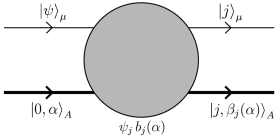
Figure 1: Feynman diagram for a transition from the initial state $\lvert\psi\rangle_{\mu}\otimes\lvert 0,\alpha\rangle_{A}$ to the final state $\lvert j\rangle_{\mu}\otimes\lvert j,\beta_{j}(\alpha)\rangle_{A}$, $j=\pm$. The transition amplitude $\psi_{j}b_{j}(\alpha)$ depends on the microscopic details of the initial state $\lvert 0,\alpha\rangle_{A}$ of the larger system $A$ and on the initial state $\lvert\psi\rangle_{\mu}$ of $\mu$.

In scattering theory, the interaction between $\mu$ and $A$ is characterised by the transition operator $M$, and this leads to the (non-normalized) final state (see Figure 1),

$$M\lvert\psi\rangle_{\mu}\otimes\lvert 0,\alpha\rangle_{A}=b_{+}(\alpha)\psi_{+}\lvert+\rangle_{\mu}\otimes\lvert+,\beta_{+}(\alpha)\rangle_{A}+b_{-}(\alpha)\psi_{-}\lvert-\rangle_{\mu}\otimes\lvert-,\beta_{-}(\alpha)\rangle_{A}\;.$$ (3)

In general, the amplitudes, $b_{+}(\alpha)$ and $b_{-}(\alpha)$, are not equal and therefore the proportions between $+$ and $-$ can change in a way that depends on the initial state $\lvert 0,\alpha\rangle_{A}$ of $A$. (Note that $M$ must not to be confused with the unitary scattering operator $S$; see the Supplemental Material [10].)

The requirement of a statistically unbiased measurement means that $\langle\langle|b_{+}|^{2}\rangle\rangle=\langle\langle|b_{-}|^{2}\rangle\rangle$, where $\langle\langle\;\rangle\rangle$ denotes mean value over the ensemble of initial states $\lvert 0,\alpha\rangle_{A}$ of $A$.

Equation (3) describes a mechanism of the measurement process in which von Neumann’s dilemma is not present. Since relativistic quantum mechanics, in the form of scattering theory of quantum field theory, is a more correct theory than the non-relativistic Schrödinger equation, as it was used in the 1930s, we choose to use Equation (3) as our starting point.

In quantum field theory, the two channels are connected via the initial state and inverse processes. A formulation based on perturbation theory with Feynman diagram representation to all orders, leads to an explicitly unitary description of the whole process. (This is shown in the Supplemental Material [10].)

For equation (3) to properly represent a measurement process, i.e., a bifurcation that leads to a final state with $\mu$ in either of the eigenstates of $\sigma_{3}$, it is necessary that the squared moduli of the amplitudes satisfy either $|b_{+}|^{2}>>|b_{-}|^{2}$ or $|b_{-}|^{2}>>|b_{+}|^{2}$. If this holds for (almost) all microstates $\alpha$ in the resulting ensemble of final states, it can function as a mechanism for the bifurcation of the measurement process.

The von Neumann dilemma came from assuming $A$ to be in a given initial state $\lvert 0,\alpha\rangle_{A}$. For the initial state of $\mu A$-interaction, $A$ can be in any of the states of the available initial ensemble. These states are ready to influence the recording process in different ways. To reach a final state, given by Equation (3), they compete with their transition rates, $(2\pi)^{-1}\big{(}|\psi_{+}|^{2}|b_{+}(\alpha)|^{2}+|\psi_{-}|^{2}|b_{-}(\alpha)|^{2}\big{)}$, which can differ widely between different values of $\alpha$. The competition leads to a selection and to a statistical distribution over $\alpha$ of the final states that is very different from the distribution in the initial ensemble.

It remains to be shown how the bifurcation leading to either $+$ or $-$ can occur, i.e., how we get either $|b_{+}|^{2}>>|b_{-}|^{2}$ or $|b_{-}|^{2}>>|b_{+}|^{2}$.

If this can be shown, however, we can see already now that because $\langle\langle|b_{+}|^{2}\rangle\rangle=\langle\langle|b_{-}|^{2}\rangle\rangle$, in the mean, the partial transition rates, $(2\pi)^{-1}|\psi_{+}|^{2}|b_{+}(\alpha)|^{2}$ and $(2\pi)^{-1}|\psi_{-}|^{2}|b_{-}(\alpha)|^{2}$, are proportional to $|\psi_{+}|^{2}$ and $|\psi_{-}|^{2}$, which thus are the probabilities for the final results $+$ or $-$. This means that under the stated condition, we have obtained Born’s rule.

Schematic mathematical model of a measurement device.—Up till now, we have used only very general features of scattering theory. In order to illustrate how microscopic details of the measurement device may result in domination of either of the transition amplitudes $b_{\pm}$, we construct a schematic model of a measurement device of stepwise increasing size. It is assumed that each step contributes a factor, close to $1$, depending on microscopic details $\alpha$ of the device, so that after $N$ steps we have a resulting product of $N$ independent factors. For simplicity, we assume that each factor is enhancing one channel and suppressing the other. Mathematically, this can be expressed as

$$|b_{+}(\alpha)|^{2}=\prod_{n=1}^{N}\big{(}1+\kappa_{n}(\alpha)\big{)}=e^{\Xi(Y(\alpha)-\tfrac{1}{2})}\;,$$ (4)

$$|b_{-}(\alpha)|^{2}=\prod_{n=1}^{N}\big{(}1-\kappa_{n}(\alpha)\big{)}=e^{\Xi(-Y(\alpha)-\tfrac{1}{2})}\;,$$

where $\kappa_{n}(\alpha)^{*}=\kappa_{n}(\alpha)$, and where the small deviations from unity in the factors are characterised by $\langle\langle\kappa_{n}\rangle\rangle=0$, $\langle\langle\kappa_{n}\kappa_{n^{\prime}}\rangle\rangle=\delta_{nn^{\prime}}\kappa^{2}$, $0<\kappa<<1$, and $\Xi=N\kappa^{2}$. We have followed the convention to calculate to second order in $\kappa_{n}$ and then replace $\kappa_{n}\kappa_{n^{\prime}}$ by its mean $\delta_{nn^{\prime}}\kappa^{2}$. In (4), we have introduced the aggregate variable,

$$Y(\alpha)=\frac{1}{\Xi}\sum_{n=1}^{N}\kappa_{n}\;.$$ (5)

representing the overall degree of enhancement/suppression (so that $Y>0$ for net enhancement of $+$ and $Y<0$ for net enhancement of $-$). The resulting squared amplitudes in (4) have the means unity, $\langle\langle|b_{\pm}|^{2}\rangle\rangle=\langle\langle e^{\Xi(\pm Y-\tfrac{1}{2})}\rangle\rangle=1$. An extra common factor for the amplitudes would not make any difference. For $Y$ in (5), the mean and variance are $\langle\langle Y\rangle\rangle=0$ and $\langle\langle Y^{2}\rangle\rangle=\Xi^{-1}$.

For a large $\Xi$, i.e., for a sufficiently large number $N$, and a non-zero $Y$, the ratio of the squared moduli of the amplitudes $|b_{+}|^{2}/|b_{-}|^{2}=e^{2\Xi Y}$ becomes very large or very small. This demonstrates how the bifurcation can result from the unknown details of the initial state of the apparatus. Thus the condition for $\mu$ ending up in an eigenstate of $\sigma_{3}$ is fulfilled; our reasoning above showed that under the same condition, the eigenstates are reached with probabilities given by Born’s rule.

In order to see all this more in detail for our model, we discuss the statistics of initial states and final states. Since all steps of extension in (4) are independent, the distribution over the aggregate variable $Y$, defined by Equation (5), in the ensemble of initial states of $A$, is well described by the Gaussian distribution,

$$q(Y)=\sqrt{\frac{\Xi}{2\pi}}\;e^{-\tfrac{1}{2}\Xi Y^{2}}\;.$$ (6)

The rate of the transition (3) with $|b_{\pm}|^{2}$ given by (4) is $(2\pi)^{-1}w(Y)$ where

$$w(Y)=|\psi_{+}|^{2}e^{\Xi(Y-\tfrac{1}{2})}+|\psi_{-}|^{2}e^{\Xi(-Y-\tfrac{1}{2})}\;,$$ (7)

with $\langle\langle w(Y)\rangle\rangle=1$. In (7), the first term is the transition rate to the state $\lvert+\rangle_{\mu}\otimes\lvert+,\beta_{+}(\alpha)\rangle_{A}$ and the second term is the rate to the state $\lvert-\rangle_{\mu}\otimes\lvert-,\beta_{-}(\alpha)\rangle_{A}$.

The total transition rate (7) depends strongly on $Y$. We shall now go into the statistics of the final states which is strongly influenced by $w(Y)$. To get the distribution $Q(Y)$ over $Y$ for the final states, corresponding to $q(Y)$ for the initial states, we must multiply $q(Y)$ by the transition rate (7) which is normalized in the sense that its mean value is $1$. This is the standard approach in scattering theory, see, e.g., Ref. [11]. Here, it can be interpreted as a selection process, as previously discussed, that favours initial states that are efficient in leading to a transition, with a selective fitness being proportional to the transition rate (7). We then get (see Figure 2)

$$Q(Y)=q(Y)w(Y)=|\psi_{+}|^{2}Q_{+}(Y)+|\psi_{-}|^{2}Q_{-}(Y)\;,$$

$$Q_{\pm}(Y)=\sqrt{\frac{\Xi}{2\pi}}\;e^{-\tfrac{1}{2}\Xi(Y\mp 1)^{2}}\;.$$ (8)

The normalized partial distributions, $Q_{+}(Y)$ and $Q_{-}(Y)$, also with variance $\Xi^{-1}$, are centered around $Y=1$ and $Y=-1$ and correspond to $\mu$ ending up in the state $\lvert+\rangle_{\mu}$ and $\lvert-\rangle_{\mu}$, respectively. The coefficients of $Q_{+}(Y)$ and $Q_{-}(Y)$ in (Q(Y)), $|\psi_{+}|^{2}$ and $|\psi_{-}|^{2}$, express Born’s rule explicitly.

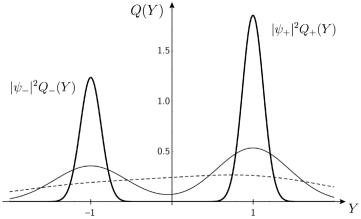
Figure 2: The distribution $Q(Y)$ over $Y$ of transitions taking place in $\mu A$-interaction for increasing size of $A$ corresponding to $\Xi=1$ (broken line), $\Xi=5$ (thin line), and $\Xi=60$ (thick line). $Q(Y)$ is composed of two distributions $Q_{+}(Y)$ and $Q_{-}(Y)$ with weights $|\psi_{+}|^{2}$ and $|\psi_{-}|^{2}$, respectively. These distributions become separated as $\Xi$ increases. Each initial state of $A$, $\lvert 0,\alpha\rangle_{A}$, is represented by a certain $Y=Y(\alpha)$. As the size of the measurement device increases and $\Xi$ becomes larger, states that are efficient in leading to a transition are found around $Y=-1$ and $Y=+1$, respectively. These initial states then lead to $\mu$ ending up in either $\lvert-\rangle_{\mu}$ or $\lvert+\rangle_{\mu}$, respectively, with probabilities confirming the Born rule.

It is instructive to follow the distribution $Q(Y)$ with growing $\Xi$. For small $\Xi$ ($=N\kappa^{2}$) it is broad and unimodal; it then turns broad and bimodal with narrowing peaks. For large $\Xi$, it is split into two well separated distributions with sharp peaks, weighted by the squared moduli of the state components of $\mu$, $|\psi_{+}|^{2}Q_{+}(Y)$ and $|\psi_{-}|^{2}Q_{-}(Y)$, at $Y=1$ and $Y=-1$, respectively. They represent two different subensembles of final states (see Equation (2)). Other values of $Y$ correspond to non-competitive processes. The aggregate variable $Y$ is ”hidden” in the fine unknown details of $A$ that can influence the $\mu A$-interaction.

The initial state for $\mu$ in (1) is a superposition, a ’both-and state’, and it ends up in (2) which is again a product state, with $\mu$ in either $\lvert+\rangle_{\mu}$ or $\lvert-\rangle_{\mu}$. The initial states of $A$ vary widely in their efficiency to lead to a final state. When one transition-rate term in (7) is large, the other one is small. The selection of a large transition rate therefore also leads to a bifurcation with one of the terms in (3) totally dominating the final state.

Generic model of $A$ and the $\mu A$-interaction.—To give some hint of the physical meaning of our mathematical modelling, we sketch a generic model for $A$. We let $\mu$ be a fast incoming electron in a prepared spin state. To measure $\sigma_{3}$, we separate the $\lvert+\rangle_{\mu}$ and the $\lvert-\rangle_{\mu}$ components in an inhomogeneous magnetic field and send the $\lvert+\rangle_{\mu}$ component into a detector where $\mu$ has a possibility to initiate a visible track by ionizing molecules along its path. The $\lvert-\rangle_{\mu}$ component is led outside the detector and thus $b_{-}(\alpha)=1$. In this respect our example differs from the model of Equation (4). A recorded detection means the result $+$; no detection means the result $-$.

We think of the component of $\mu$ passing through the detector as a small wavepacket; we let $A$ be a small cylinder of the detector material around the path of the wavepacket. We take successive small steps to build up $A$ by small increases of the cylinder diameter. Each unknown factor in the squared amplitude $|b_{+}|^{2}$, of Equation (4), coming from an extension of $A$, makes $|b_{+}|^{2}$ grow or shrink while $|b_{-}|^{2}=1$. Also in this case $\langle\langle|b_{+}|^{2}\rangle\rangle=1$ expresses the metastability of $A$.

What starts as a state of $A$ with small components with ionized molecules along the path of $\mu$ can either develop into a state with sufficient seeds for condensation or boiling or relax back into a state of neutral molecules. An ambivalence in the selection of these alternatives is constitutional for the necessary metastability of the detector. The parameters $\kappa_{n}(\alpha)$ model this ambivalence in the transition amplitudes to a final state for $A$. These parameters depend on fine accidental details of its ingoing state $\lvert 0,\alpha\rangle_{A}$.

Discussion.—In our description, we want the system $A$ to be big enough for a bifurcation to take place. We leave out the irreversible development beyond $A$. Our idea is to follow the qualitative recipe given by Bell who formulated a principle concerning the position of the Heisenberg cut [9], i.e., the boundary of the system $A$, interacting with $\mu$ according to quantum dynamics (Ref. [9], p.124):

put sufficiently much into the quantum system that the inclusion of more would not significantly alter practical predictions

In the model that we have described, the bifurcation of measurement takes place in the reversible stage of the interaction between $\mu$ and $A$ before irreversibility sets in and fixes the result. In this respect, our analysis is very different from decoherence analysis [12, 13] and also from the approach in Zurek’s work [14], where the bifurcation is considered as a part of an irreversible process.

The system $A$ should not be so large that $\mu\cup A$ cannot be described by deterministic quantum dynamics. Still, it must be possible to have the entanglement process sufficiently extensive, i.e., to have $\Xi=N\kappa^{2}$ sufficiently large. Then we have followed Bell’s principle quoted above concerning the position of the Heisenberg cut.

For future work, a more detailed description is needed of a typical $\mu A$-interaction, including the statistics of the initial states and the selection of one state $\lvert 0,\alpha\rangle_{A}$ with a large transition amplitude, leading to a final state (2) with $\mu$ in one eigenstate, $\lvert+\rangle_{\mu}$ or $\lvert-\rangle_{\mu}$. An important task is to construct a detailed physical model of a non-biased measurement apparatus like the one sketched above.

So far, the unitarity of the scattering matrix has not been explicitly visible. Reversibility that we have pointed out as crucial, is also not explicit. To remedy this we have made a slightly more elaborate description of the whole process where the observed system $\mu$ is produced in its initial state $\lvert\psi\rangle_{\mu}$ by an external source before interaction with $A$ and absorbed by a sink in one of the possible final states after the interaction. Then both unitarity and reversibility are made explicit. The calculation has been done through evaluation of Feynman diagrams summed to all orders in perturbation theory. (This version is presented in the Supplemental Material [10].)

We have also checked that it is straightforward to generalize our model to (i) any number of possible measurement results, and (ii) a system $A$ entangled with its environment and not possible to describe as being in a pure initial state.

If we had shown the development of $|b_{\pm}|^{2}$ for each step instead of going directly to the resulting product in Equation (4), in mathematical terms, we would have seen a quantum diffusion process close to the one described by Gisin and Percival [4, 5, 6].

In earlier work, non-linearities have sometimes been brought in through generalization of quantum mechanics. Besides the quantum diffusion model, the Ghirardi-Rimini-Weber model is of this kind [7, 8]. In our model, we have seen how non-linearities can arise within quantum mechanics as higher-order terms in a perturbation expansion without any generalization.

In practical scientific research, there is a common working understanding of quantum mechanics. Physicists have a common reality concept for a quantum-mechanical system when it is not observed, a kind of pragmatic quantum ontology with the quantum-mechanical state of the studied system as the basic concept. Development of this state in time then constitutes the quantum dynamics. If quantum mechanics now can also be used to describe the measurement process, this pragmatic quantum ontology can have a wider validity than has been commonly expected.

Quantum mechanics deserves to be recognized as a realistic and deterministic theory and not only considered as a set of calculation rules with some spooky or weird features. A better understanding of quantum mechanics is essential at a time of fast progress both in experimental knowledge of quantum processes and in quantum technology.

References

- [1] M. Nauenberg. Does quantum mechanics require a conscious observer? Journal of Cosmology, 14, 2011.
- [2] H. Everett. “Relative state” formulation of quantum mechanics. Reviews of Modern Physics, 29:454, 1957.
- [3] B. S. DeWitt. Quantum mechanics and reality. Physics Today, 23:30–35, 1970.
- [4] N. Gisin. Quantum measurements and stochastic processes. Physical Review Letters, 52:1657, 1984.
- [5] N. Gisin and I. C. Percival. The quantum-state diffusion model applied to open systems. Journal of Physics A: Mathematical and General Phys. A: Math. Gen., 25:5677–5691, 1992.
- [6] I. C. Percival. Primary state diffusion. Proceedings of the Royal Society of London, A, 447:189–209, 1994.
- [7] G. C. Ghirardi, A. Rimini, and T. Weber. Unified dynamics for microscopic and macroscopic systems. Physical Review D, 34:470, 1986.
- [8] G. C. Ghirardi, P. Pearle, and A. Rimini. Markov processes in Hilbert space and continuous spontaneous localization of systems of identical particles. Physical Review A, 42:78, 1990.
- [9] J. S. Bell. Speakable and Unspeakable in Quantum Mechanics, chapter Quantum Mechanics for Cosmologists. Cambridge University Press, 2nd edition, 2004.
- [10] See Supplemental Material that includes a clarification of the role of the scattering and the transition matrices, a detailed description of the statistics of final states, a Feynman diagram representation of the model that makes inverse processes and unitarity explicit, and a number of relevant citations from the history of quantum measurement.
- [11] J. Jauch and F. Rohrlich. The Theory of Photons and Electrons (Sect. 8-6). Addison-Wesley, 1955.
- [12] H. D. Zeh. On the interpretation of measurement in quantum theory. Foundations of Physics, 1:69–76, 1970.
- [13] M. Schlosshauer. Decoherence, the measurement problem, and interpretations of quantum mechanics. Reviews of Modern Physics, 76:1267–1305, 2005.
- [14] W. H. Zurek. Decoherence, einselection, and the quantum origins of the classical. Reviews of Modern Physics, 75:715–775, 2003.
- [15] K.-E. Eriksson, M. Cederwall, K. Lindgren, and E. Sjöqvist. Bifurcation in quantum measurement. arXiv:1708.01552v2 [quant-ph], 2017.