Modelling carbon-chain species formation in lukewarm corinos with new multi-phase models

Abstract

Context. Abundant carbon-chain species have been observed towards lukewarm corinos L1527, B228, and L483. These carbon-chain species are believed to be synthesized in the gas phase after CH₄ desorbs from the dust grain surface at the temperature around 30 K.

Aims. We investigate carbon-chain species formation in lukewarm corinos using a more rigorous numerical method and advanced surface chemical models. We also pay attention to the significance of the finite size effect.

Methods. We used the macroscopic Monte Carlo method in our simulations. In addition to the two-phase model, the basic multi-phase model and the new multi-phase models were used for modelling surface chemistry on dust grains. All volatile species can sublime at their sublimation temperatures in the two-phase model while most volatile species are frozen in the ice mantle before water ice sublimes in the basic and the new multi-phase models. The new multi-phase models allow more volatile species to sublime at their sublimation temperatures than the basic multi-phase model does.

Results. The significance of the finite size effect is dependent on the duration of the cold phase. The discrepancies between the rate equation approach and the Monte Carlo method decrease as the duration of the cold phase increases. When $T\sim 30\,\mathrm{K}$, the abundances of gaseous CH₄ and CO in the two-phase model are the highest while the basic multi-phase model predicts the lowest CO and CH₄ abundances among all models. The abundances of carbon-chain species in the basic and the new multi-phase models are lower than that in the two-phase model when $T\sim 30\,\mathrm{K}$ because CH₄ is crucial for the synthesis of carbon-chain species. However, because the abundance of electrons increases as the abundance of H₃O⁺ decreases, some carbon-chain species abundances predicted by the basic multi-phase model may not be lower than that in the new multi-phase models. The two-phase model performs best in predicting carbon-chain species abundances to fit observations while the basic multi-phase model works the worst. The abundances of carbon-chain species predicted by the new multi-phase models agree reasonably well with observations.

Conclusions. The amount of CH₄ that can diffuse inside the ice mantle, thus sublime upon warm-up plays a crucial role in the synthesis of carbon-chain species in the gas phase. The carbon-chain species observed in lukewarm corinos may be able to gauge surface chemical models.

1 Introduction

Abundant carbon-chain molecules have been observed in the early stage of low-mass star forming regions which are known as lukewarm corinos. The mechanism for synthesizing carbon-chain molecules in these sources is known as warm carbon-chain chemistry (WCCC) (Sakai et al., 2008), therefore the lukewarm corinos with abundant carbon-chain molecules are also called WCCC sources. L1527 in Taurus is confirmed to be the first WCCC source (Sakai et al., 2008), which contains the low-mass protostar IRAS 04368+2557 in the transitional phase from Class 0 to Class I (Andre et al., 2000; Hassel et al., 2008; Sakai et al., 2009b, 2010). So far 14 carbon-chain species with relatively high abundances have been observed towards L1527. IRAS 15398-3359 in Lupus, which is also identified as B228, is confirmed as the second WCCC source (Sakai et al., 2009a). This protostar is also in the transitional phase from Class 0 to Class I. Six carbon-chain species have been observed towards B228. Recently, abundant carbon-chain species as well as more saturated complex organic molecules (COMs) are observed towards L483 (Oya et al., 2017) in the Aquila Rift. This cloud contains the Class 0 protostar IRAS 18148-0440 (Fuller et al., 1995). Other possible WCCC sources include B1, L1448N (Sakai et al., 2009a; Hassel et al., 2011), and the L1251A molecular core around the Class 0 protostar L1251A IRS3 (Cordiner et al., 2011).

The discovery of abundant carbon-chain species in low-mass star forming regions is unexpected because these species are characteristics of dark clouds (Suzuki et al., 1992; Hassel et al., 2008; Sakai et al., 2008). Before abundant carbon-chain species were observed towards L1527, COMs have been observed towards low-mass star forming regions (Cazaux et al., 2003; Bottinelli et al., 2004; Jørgensen et al., 2005; Sakai et al., 2006; Bottinelli et al., 2007; Jørgensen et al., 2012; Maury et al., 2014; Taquet et al., 2015). These low-mass star forming regions with COMs are known as hot corinos, which are warmer than the lukewarm corinos. The desorption of CH₄ is the first step to synthesize carbon-chain species in the lukewarm corinos according to the WCCC mechanism (Sakai et al., 2008, 2009a; Lindberg et al., 2016). When the temperature arises to about 30 K, volatile species such as CH₄ can sublime from the grain surface. The sublimated species participate in gas phase reactions to produce carbon-chain species. So far, carbon-chain species abundances predicted by chemical models for L1527 agree reasonably well with observations (Aikawa et al., 2008; Hassel et al., 2008, 2011). However, further modelling studies on WCCC are necessary because of the limitations of previous models.

First, some previous models use the rate equation (RE) approach in the numerical simulations which in some cases may be problematic. When the average population of reactive species on the grain surface is well below one, the RE approach can lead to large errors in the simulation results (Tielens & Charnley, 1997). This problem is known as the finite size effect. Vasyunin et al. (2009) showed that the abundances of species predicted by the RE approach deviate much from that by the more rigorous macroscopic Monte Carlo (MC) approach if the temperature is within 20 K and 50 K. Although previous WCCC model results at about 30 K agree with observations (Hassel et al., 2008), it is questionable whether the model results simulated with the more rigorous numerical approach still fit the observations well.

Second, a more serious problem with previous WCCC simulations is the way their models treat the surface chemistry. All volatile species such as CH₄ and CO in the ice mantle of a dust grain are assumed to sublime when the temperature is higher than their sublimation temperatures in these models. However, laboratory experiments show that not all CO can desorb when the temperature is higher than the CO sublimation temperature (Sandford & Allamandola, 1988; Collings et al., 2003). There is also observational evidence that CO might be trapped in the ice mantle. For instance, the abundance of CO in some prestellar cores is observed to be lower than its canonical value (Fuente et al., 2012), and one possible explanation is that CO is trapped in the ice mantle. As the sublimation of CH₄ triggers the synthesis of carbon-chain species in the gas phase, the production of carbon-chain species may be less efficient if a fraction of CH₄ molecules are locked in the ice mantle.

More advanced surface chemical models are necessary so that the trapped CH₄ in the mantle at temperatures higher than 30 K is considered. All previous WCCC models have adopted the widely used two-phase model in which all surface species can participate in reactions including sublimation. In order to consider the trapping effect, a more advanced model called the three-phase model was suggested by Hasegawa & Herbst (1993). This model distinguishes species on the grain surface active layers and species buried in the ice mantle. Species in the active layers are reactive while species in the ice mantle are chemically inert. As the temperature increases, only species in the active layers can sublime, thus the majority of solid species are trapped in the ice mantle. The original three-phase model was simulated using the RE approach, but recently, Vasyunin & Herbst (2013) performed more rigorous macroscopic MC simulations of the three-phase model. However, the assumption in the three-phase model that species in the bulk of ice are completely inert may not be correct. For example, it is estimated that the probability that photons are absorbed by one monolayer of ice is about 0.007 (Andersson & van Dishoeck, 2008). Thus photons can easily penetrate through about 150 monolayers of ice and photo-dissociate species deeply buried in the ice mantle. A few modified three-phase models that adopt a partially active bulk ice mantle are suggested (Garrod, 2013a; Chang & Herbst, 2014; Kalvāns et al., 2017; Lu et al., 2018). Moreover, in the model suggested by Lu et al. (2018), the exponential decay with depth of photolysis in the ice mantle is well mimicked.

In this work, we have investigated WCCC using the macroscopic MC method and the advanced surface chemical models. We are particularly interested in studying the carbon-chain species abundances predicted by different surface models. The models used in this work are the two-phase model, the three-phase model suggested by Vasyunin & Herbst (2013), and the new multi-phase models suggested by Lu et al. (2018).

In Sect. 2 we describe our chemical models and the physical model of lukewarm corinos. In Sect. 3 we present all model results. In Sect. 4 we compare the results with observations. In Sect. 5 we discuss the advantages and disadvantages of different models and present our conclusions.

2 Model

2.1 Chemical model

Table 1: Model parameters.

Parameter	Symbol	Value
Sticking coefficient	$P_{\mathrm{s}}$	0.5
Reactive desorption efficiency	$a_{\mathrm{RRK}}$	0.01
Ratio of surface diffusion barriers to desorption energies	$E_{\mathrm{b1}}/E_{\mathrm{d}}$	0.5
Ratio of bulk diffusion barriers to desorption energies	$E_{\mathrm{b2}}/E_{\mathrm{d}}$	0.7
Barrier thickness	$b$	1 Å
Grain radius	$r$	0.1 $\mu$m
Dust grain density	$\rho_{\mathrm{d}}$	3 g cm-3
Dust-to-gas mass ratio	$m_{\mathrm{d/g}}$	0.01
Number of absorption sites on each grain	$S$	1.0$\times$106
Surface density of sites	$N_{\mathrm{S}}$	7.96$\times$1014 sites cm-2
Unattenuated FUV flux	$\chi$	$\chi_{0}=1$
Cosmic ray ionization rate	$\zeta_{\mathrm{CR}}$	1.3$\times$10-17 s-1
Fraction of the timescale between two cosmic-ray heating events	$f$	3.16$\times$10-19
Characteristic vibrational frequency	$\nu_{0}$	1$\times$1012 s-1

Table 2: Initial abundances (Hassel et al., 2008).

Species	$n_{\mathrm{X}}/n_{\mathrm{H}}$
H2	5.00(-1)
He	1.40(-1)
C+	7.30(-5)
N	2.14(-5)
O	1.76(-4)
S+	8.00(-8)
Na+	2.00(-9)
Mg+	7.00(-9)
Si+	8.00(-9)
P+	3.00(-9)
Cl+	4.00(-9)
Fe+	3.00(-9)

The new multi-phase model used in this work has been explained in detail by Lu et al. (2018). Here we only briefly explain the model in the following. The ice mantle on the grain surface is composed of surface active layers and a partially active bulk of ice. Species in the surface active layers can diffuse and participate in surface reactions including sublimation. There are two types of binding sites in the partially active bulk of ice, the normal sites and the interstitial sites. Species occupying normal sites are called normal species, while interstitial species occupy interstitial sites and are uniformly distributed in the partially active bulk of ice. Normal species are locked in the mantle, thus cannot sublime until the whole ice mantle sublimes, while interstitial species can diffuse in the bulk of ice and sublime at their sublimation temperatures. Interstitial species can be generated by the photolysis of species in the bulk of ice. Both the UV photons from the external radiation and that induced by cosmic ray are considered in our chemical model. Photo-fragments of icy species can enter normal sites or interstitial sites. The probability for a photo-dissociation product at the M-th layer of ice to enter the interstitial site is,

$$P=\frac{\alpha N_{emp,int}}{\alpha N_{emp,int}+N_{emp,nor,M}},$$ (1)

where $N_{emp,int}$ is the average number of empty interstitial sites, $N_{emp,nor,M}$ is the number of empty normal sites at the M-th layer, and $\alpha$ is a parameter depending on the difference of the binding energy of normal sites and interstitial sites. The larger the parameter $\alpha$ is, the more likely that photo-dissociation products occupy interstitial sites and, therefore, the more interstitial volatile species can sublime as the temperature increases. However, the parameter $\alpha$ is poorly known so far. Lu et al. (2018) argued that $\alpha$ should be no more than one, thus we set $\alpha$ to be 1, 0.5, and 0.01 in the new multi-phase models. Moreover, we also simulate a new multi-phase model in which all photo-dissociation products enter interstitial sites ($\alpha=+\infty$) to maximize the population of interstitial species in the model. New multi-phase models adopting $\alpha=+\infty$, 1, 0.5, and 0.01 are called new multi-phase model 0, 1, 2, and 3 in this work, respectively. We also simulated the two-phase model and the three-phase model suggested by Vasyunin & Herbst (2013), which is referred to as the basic multi-phase model in this work. The amounts of CH₄ that can sublime at the CH₄ sublimation temperature are different in these models. In the basic multi-phase model, CH₄ molecules only in the active layers can sublime while all surface CH₄ can desorb in the two-phase model. The amount of CH₄ molecules that can sublime in the new multi-phase model is larger than that in the basic multi-phase model but less than that in the two-phase model, because CH₄ molecules in the active layers and those occupying interstitial sites can sublime at the CH₄ sublimation temperature in the new multi-phase models. Therefore, among all the models, carbon-chain species in the two-phase model should be the most abundant while the abundances of carbon-chain species predicted by the basic multi-phase model should be the lowest.

The macroscopic MC method is used to simulate the two-phase model, the basic multi-phase model and the new multi-phase models. Following Vasyunin et al. (2009), we isolate a cell of gas surrounding a dust particle. The total population of H nuclei is $10^{12}$ in the cell of gas if we set $\rho_{\mathrm{d}}$ = 3 g cm^-3 and $m_{\mathrm{d/g}}$ = 0.01 (Vasyunin et al., 2009). In this work, we report the fractional abundance of species, which is defined as the ratio of the population of the species to total population of H nuclei (10¹²) in the cell. If the population of a species is one, its fractional abundance is 10^-12. This abundance is the minimum fractional abundance resolvable if we run a model only once. In order to reduce statistical fluctuation, we ran each model ten times to calculate the average fractional abundances, so the lowest fractional abundance resolvable is 10^-13. Any fractional abundance lower than 10^-13 is reported to be zero in this paper. In order to research the finite size effect, we also use the RE approach to simulate the two-phase model for comparison.

We performed the macroscopic MC simulations of the gas-grain chemical reaction network used by Hassel et al. (2008) (hereafter HHG), which is based on the OSU2008 reaction network but with some changes, and found that even in the two-phase model, carbon-chain species may be severely underproduced. The abundances of carbon-chain species in the two-phase model using a reaction network that includes all reactions in the OSU2008 and HHG agree with observations better than that using OSU2008 or HHG individually, therefore the combined reaction network is utilized in all models in this work. As a result, the gas-grain chemical reaction network includes 6462 reactions and 655 species. The competition mechanism is utilized to calculate the reaction rates for two surface reactions with barriers, CO + H $\rightarrow$ HCO and H₂CO + H $\rightarrow$ H₃CO (Chang & Herbst, 2012). The reaction barriers of these two reactions are taken from Fuchs et al. (2009). Finally, the accretion of H₂ consumes too much CPU time in the macroscopic MC simulations. However, it is found that H₂ accretion is not important for the molecular evolution of dense clouds (Chang et al., 2017). Thus, H₂ accretion is not included in our chemical reaction network in order to reduce the computational cost. The bulk diffusion barrier for an interstitial species is set to be $E_{\mathrm{b2}}=0.7E_{\mathrm{d}}$ (Lu et al., 2018), where $E_{\mathrm{d}}$ is the desorption energy of the same species in the active layers. All other parameters in the network are the same as that used by Hassel et al. (2008) and Semenov et al. (2010), which are shown in Table 1. We adopted the low initial metal abundances as shown in Table 2 (Hassel et al., 2008).

Table 3: $\Delta t$ and the corresponding temperatures when the abundances of HC₅N, HC₇N and HC₉N reach $10^{-12}$ in the two-phase model adopting different $t_{\mathrm{cold}}$ values.

$t_{\mathrm{cold}}$ (yr)	HC5N		HC7N		HC9N
	$\Delta t$ (yr)	$T$ (K)	$\Delta t$ (yr)	$T$ (K)	$\Delta t$ (yr)	$T$ (K)
MC $1.0\times 10^{5}$	$6.97\times 10^{4}$	33.08	$7.72\times 10^{4}$	38.31	$9.96\times 10^{4}$	57.12
MC $2.0\times 10^{5}$	$6.01\times 10^{4}$	27.16	$7.05\times 10^{4}$	33.61	$7.55\times 10^{4}$	37.08
MC $3.0\times 10^{5}$	$4.78\times 10^{4}$	20.85	$5.60\times 10^{4}$	24.90	$5.81\times 10^{4}$	26.03
MC $4.0\times 10^{5}$	$4.26\times 10^{4}$	18.62	$5.60\times 10^{4}$	24.90	$5.72\times 10^{4}$	25.54
MC $5.0\times 10^{5}$	$4.55\times 10^{4}$	19.83	$5.67\times 10^{4}$	25.27	$5.97\times 10^{4}$	26.93
MC $6.0\times 10^{5}$	$4.50\times 10^{4}$	19.62	$5.83\times 10^{4}$	26.14	$5.93\times 10^{4}$	26.70
MC $7.0\times 10^{5}$	$4.53\times 10^{4}$	19.75	$5.79\times 10^{4}$	25.92	$5.96\times 10^{4}$	26.87
MC $8.0\times 10^{5}$	$4.46\times 10^{4}$	19.45	$5.82\times 10^{4}$	26.09	$6.16\times 10^{4}$	28.02
MC $9.0\times 10^{5}$	$5.07\times 10^{4}$	22.21	$5.87\times 10^{4}$	26.37	$6.29\times 10^{4}$	28.79
MC $1.0\times 10^{6}$	$4.57\times 10^{4}$	19.92	$5.75\times 10^{4}$	25.70	$6.10\times 10^{4}$	27.67
RE $1.0\times 10^{5}$	$5.40\times 10^{4}$	23.85	$5.68\times 10^{4}$	25.32	$5.96\times 10^{4}$	26.87
RE $3.0\times 10^{5}$	$5.23\times 10^{4}$	22.99	$5.87\times 10^{4}$	26.37	$5.87\times 10^{4}$	26.37

2.2 Physical model

We adopted the physical model used by Hassel et al. (2008), which is a homogeneous one-point model that includes two stages, a cold phase when the temperature of the molecular cloud is 10 K at the beginning and then a warm-up phase. In this model, the total hydrogen nucleus density is $n_{\mathrm{H}}=10^{6}\,\mathrm{cm}^{-3}$ in the central region of the prestellar core and the visual extinction $A_{\mathrm{V}}=10$. The initial temperature is $T=10\,\mathrm{K}$ meanwhile the gas temperature and the grain temperature are in equilibrium all the time for simplicity. The timescale of the cold phase $t_{\mathrm{cold}}$, when the temperature of the molecular cloud remains to be 10 K, is not well constrained. Hassel et al. (2008) argued through rate equation simulations that their two-phase model results are robust for the range $10^{4}$ yr $<t_{\mathrm{cold}}<$ $10^{6}$ yr, thus they suggest a moderate value, $t_{\mathrm{cold}}=10^{5}\,\mathrm{yr}$. However, we find that the results of the two-phase model simulated with the macroscopic MC method are dependent on $t_{\mathrm{cold}}$. Therefore, we simulate the two-phase model with the macroscopic MC method with different $t_{\mathrm{cold}}$ and select a moderate value of $t_{\mathrm{cold}}$ so that the predicted carbon-chain species abundances agree reasonably well with observations. Following Garrod & Herbst (2006) and Hassel et al. (2008, 2011), the temperature at the time $t_{\mathrm{cold}}$ + $\Delta t$ in the warm-up phase is,

$$T=T_{0}+(T_{\mathrm{max}}-T_{0})\left(\frac{\Delta t}{t_{\mathrm{h}}}\right)^{n},$$ (2)

where $T_{0}$ is the initial temperature, 10 K, $T_{\mathrm{max}}$ is the maximum temperature at the end of the warm-up phase that is adopted to be 200 K for the formation of hot cores or hot corinos, $t_{\mathrm{h}}$ is the heating timescale, and $n$ is the order of the heating. According to Garrod & Herbst (2006) and Hassel et al. (2008, 2011), $t_{\mathrm{h}}=2\times 10^{5}\,\mathrm{yr}$ as the timescale for intermediate star formation which is derived from the observed protostellar luminosity function (Molinari et al., 2000), and $n=2$ for power law temperature profiles (Garrod & Herbst, 2006). After the warm-up phase, the temperature remains constant.

3 Results

In this section, we report the fractional abundances of carbon-chain species in different models. The finite size effect in the two-phase model is investigated in Sect. 3.1 through a comparison of the simulation results from the macroscopic MC method and the RE approach. The two-phase, the basic and the new multi-phase models are simulated with the macroscopic MC method, and the results from these models are compared in Sect. 3.2.

3.1 Finite size effect

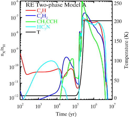
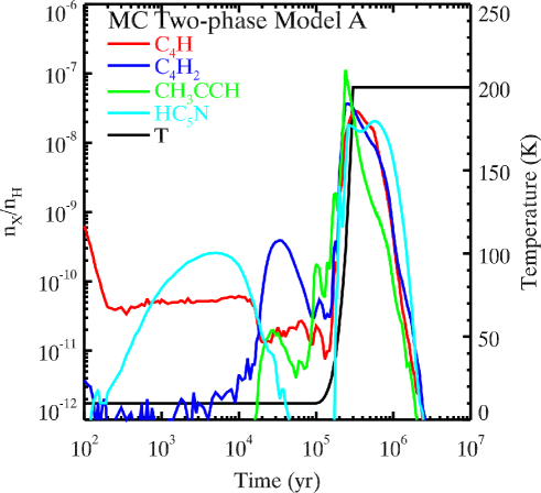
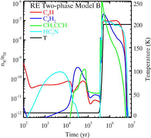
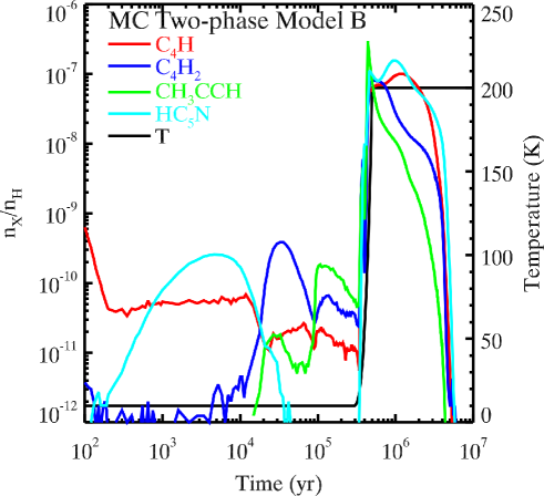
Figure 1: Temporal evolution of the fractional abundances of selected carbon-chain species in the two-phase model simulated with the RE approach and the macroscopic MC method. RE represents the rate equation calculation and MC represents the macroscopic Monte Carlo simulation. The two-phase model adopts different $t_{\mathrm{cold}}$, $t_{\mathrm{cold}}=10^{5}$ yr in the two-phase model A while $t_{\mathrm{cold}}=3\times 10^{5}$ yr in the two-phase model B. The temporal evolution of the temperature $T$ is also plotted in the figure.

The two-phase model is simulated with both the macroscopic MC method and the RE approach. The abundances of gas-phase HC₅N, HC₇N, and HC₉N in the two-phase model calculated with the RE approach deviate much from that with the macroscopic MC method. Table 3 shows $\Delta t$ in the warm-up phase and the corresponding temperatures when the abundance of HC₅N, HC₇N, and HC₉N begins to be higher than $10^{-12}$ adopting different $t_{\mathrm{cold}}$. If $t_{\mathrm{cold}}=10^{5}$ yr, the temperature has reached 33 K when the abundance of HC₅N is over $10^{-12}$ in the simulation with the macroscopic MC method. The temperature can be even higher for HC₇N and HC₉N, which increases to 38 K and 57 K, respectively. The time at which the fractional abundance is higher than $10^{-12}$, $t_{\mathrm{cold}}$ + $\Delta t$, becomes shorter so that the corresponding temperature is lower if the RE approach is used. For instance, the abundance of HC₉N starts to be higher than $10^{-12}$ when the temperature is 27 K if $t_{\mathrm{cold}}=10^{5}$ yr. These differences arise from the fact that the macroscopic MC method takes into account the finite effect while the RE approach does not (Vasyunin et al., 2009). Our results agree with previous studies in that the discrepancies of some gas phase carbon-chain species abundances between the macroscopic MC method and the RE approach can be significant when $T=25-30\,\mathrm{K}$ (Vasyunin et al., 2009). Therefore, the finite size effect is important if $t_{\mathrm{cold}}=10^{5}$ yr. On the other hand, the finite size effect becomes less important for longer $t_{\mathrm{cold}}$. If $t_{\mathrm{cold}}=3\times 10^{5}$ yr, the temperatures of the core are about 21 K, 25 K, and 26 K, respectively, when the abundances of HC₅N, HC₇N, and HC₉N are over $10^{-12}$ in the simulations with the macroscopic MC method. The RE approach predicts similar temperatures of the core, which are 23 K, 26 K, and 26 K, respectively. Moreover, in our simulations the temperatures are relatively robust if $t_{\mathrm{cold}}>3\times 10^{5}$ yr. The reason for the decrease of the discrepancy between the RE and the macroscopic MC model results as $t_{\mathrm{cold}}$ increases is that as the population of surface species increases, it becomes less likely that the average number of a surface species drops well below one, thus the finite size effect becomes less significant. In order for the abundances of carbon-chain species to be higher than $10^{-12}$ when the temperatures of the core are around 30 K in the MC models, $t_{\mathrm{cold}}$ should be no shorter than $3\times 10^{5}$ yr. Therefore, we set $t_{\mathrm{cold}}$ to be $3\times 10^{5}$ yr for all models in Sect. 3.2.

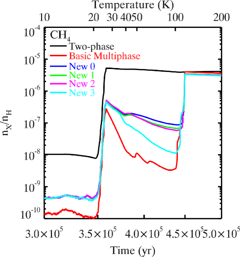
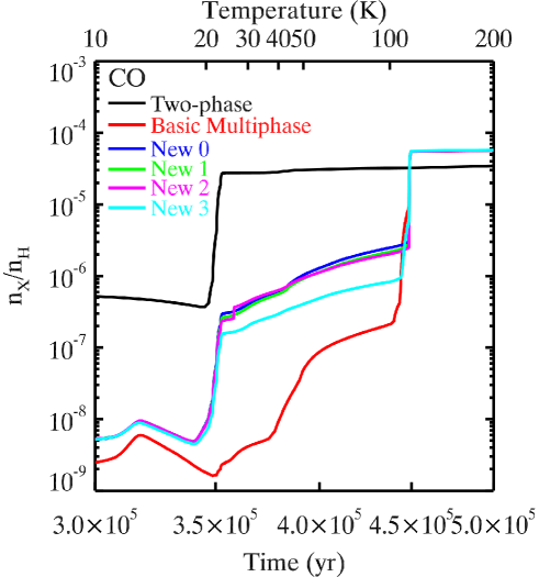
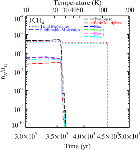
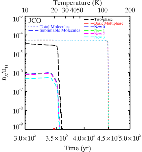
Figure 2: Temporal evolution of the fractional abundances of CH₄, CO, total JCH₄, sublimable JCH₄, total JCO, and sublimable JCO in all models. The letter J represents species on the grain. The temperature is labelled on the top horizontal axis. For total JCH₄ and JCO, the curves from all models except the two-phase model are almost the same.

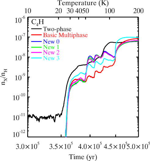
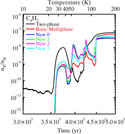
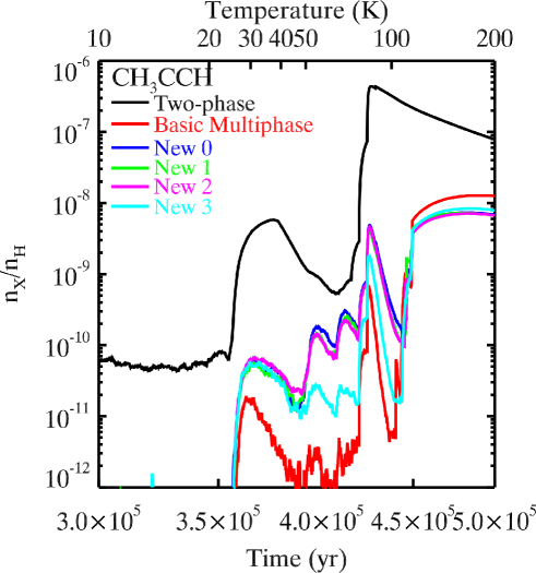
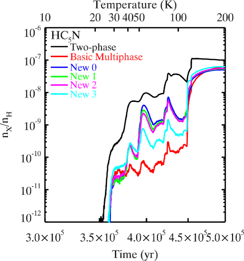
Figure 3: Temporal evolution of the fractional abundances of C₄H, C₄H₂, CH₃CCH, and HC₅N in all models. The temperature is also labelled on the top horizontal axis.

Figure 1 shows the evolutions of the abundances of selected gas-phase carbon-chain species in the two-phase model simulated with the RE approach and the macroscopic MC method. Different $t_{\mathrm{cold}}$ is used to perform the simulations. In the two-phase model A, $t_{\mathrm{cold}}$ is set to be $10^{5}$ yr while in the two-phase model B, it is $3\times 10^{5}$ yr. In an overview, the abundances of the selected carbon-chain species in the cold stage are much affected, regardless of $t_{\mathrm{cold}}$, by the numerical approach used in simulations. The finite size effect is not important at $T=10$ K in our models, which agrees with Vasyunin et al. (2009). The maximum abundances in the cold stage can reach around $4.0\times 10^{-10}$, which are relatively low in the entire evolution of 10⁷ yr. On the other hand, the abundances of carbon-chain species rise rapidly in the warm-up phase. The abundances can be more than two orders of magnitude than the peak values in the cold phase. Thus we can conclude that these carbon-chain species are synthesized rapidly during this period. Moreover, in the hot phase with $T=200\,\mathrm{K}$, the abundances decrease from the peak values to 10^-12. There are large differences between the results from the RE model and the macroscopic MC model in the warm-up phase when $t_{\mathrm{cold}}=10^{5}$ yr. The maximum abundance of CH₃CCH can be around $10^{-6}$ in the two-phase model A when the RE approach is utilized. However, the maximum abundance of CH₃CCH drops by one order of magnitude in the same model when the macroscopic MC method is used. Moreover, it takes a shorter time for the abundances of carbon-chain species to decrease to 10^-12 when the macroscopic MC method is utilized. In the RE calculations, the abundances of all selected carbon-chain species drop to 10^-12 at around $t\sim 5\times 10^{6}$ yr while in the MC simulations, carbon-chain species drop earlier at around $t\sim 2\times 10^{6}$ yr. Thus, the finite size is important when $t_{\mathrm{cold}}=10^{5}$ yr. On the other hand, the discrepancy between the RE model and the macroscopic MC model becomes smaller when longer $t_{\mathrm{cold}}$ is adopted. For instance, the maximum abundance of CH₃CCH in the two-phase model B simulated with the RE approach is only about a factor of three larger than that with the macroscopic MC method, compared with an order of magnitude in the case of a shorter $t_{\mathrm{cold}}$.

3.2 Model results comparison

Hereafter, surface species are designated by the letter J. Surface species that can sublime at their sublimation temperatures before the whole ice mantle disappears are called sublimable species. In the two-phase model all surface species are sublimable species, while in the basic multi-phase model only species in the active layers are sublimable species. In the new multi-phase models, in addition to species in the active layers, interstitial species are also sublimable species. According to Sakai et al. (2008, 2009a), CH₄ is the precursor for producing carbon-chain molecules, and CO is the precursor for producing complex organic molecules. Therefore, in order to investigate the synthesis of carbon-chain species in each model, it is important to research the abundances of sublimable JCH₄ in each model. Figure 2 shows the temporal evolution of CH₄, CO, total JCH₄, sublimable JCH₄, total JCO, and sublimable JCO in all models in the warm-up phase. The abundance of gas-phase CH₄ in the two-phase model can reach $5.2\times 10^{-6}$ when $T$ is slightly lower than 30 K, but its abundances in the new multi-phase model 0, 1, 2, and 3 can only reach around $3.0\times 10^{-7}$, which are about one order of magnitude lower than that in the two-phase model. The abundance of gaseous CH₄ in the basic multi-phase model is even lower, around $1.0\times 10^{-7}$ when $T$ is 30 K. On the other hand, the abundances of gaseous CH₄ in all models are almost the same at 200 K when all species in the ice mantle sublime. The difference of gaseous CH₄ abundance at 30 K originates from the different populations of sublimable JCH₄ molecules in these models. Although the populations of total JCH₄ in all models are approximately the same before these molecules start to sublime, the population of sublimable JCH₄ molecules in the two-phase model is about one order of magnitude higher than that in the basic multi-phase model, while in the new multi-phase models, it is a factor of between two and three larger than that in the basic multi-phase model. The populations of sublimable JCH₄ in the new multi-phase model 0-2 are approximately the same, while in the new multi-phase model 3 it is the lowest among all new multi-phase models. The same phenomenon occurs for CO. The abundance of gaseous CO in the two-phase model at 25 K is much higher than those in the basic and new multi-phase models, while gaseous CO abundances in the new multi-phase models are higher than that in the basic multi-phase model. Similarly, the abundance of sublimable JCO is the highest in the two-phase model and the lowest in the basic multi-phase model at temperatures below 25 K, and the abundances in the new multi-phase models are moderate.

Figure 3 shows the temporal evolutions of the abundances of selected gas-phase carbon-chain species in the two-phase, the basic multi-phase, and the new multi-phase models. We pay most attention to the time period when WCCC occurs at the temperature around 30 K (Hassel et al., 2008, 2011). The abundances of all selected gas-phase carbon-chain species in the new multi-phase models 0-2 are similar, which demonstrates that if $\alpha\geq 0.5$, the results of the new multi-phase models will not change much because the population of sublimable JCH₄ hardly changes as discussed before. However, these abundances in the new multi-phase model 3 do deviate from that in the other new multi-phase models. At 30 K, the new multi-phase model 3 predicts slightly lower CH₃CCH abundance and slightly higher C₄H and C₄H₂ abundances than the other new multi-phase models do. Since the abundance of gas-phase CH₄ in the new multi-phase model 3 is lower than that in the other new multi-phase models at around 30 K, less CH₃CCH are formed in the new multi-phase model 3. On the other hand, we can see that C₄H and C₄H₂ abundances in the new multi-phase model 3 are slightly higher than those in the new multi-phase models 0-2. The discrepancy can be explained as follows. Interstitial O₂ and O₃ molecules can enter active layers upon warm-up and are hydrogenated to form OH and H₂O, which may enter gas phase via reactive desorption. Both gas-phase OH and H₂O can produce H₃O⁺ ions while the electron dissociative recombination of H₃O⁺ is the major destruction pathway for electrons in our models. Because the interstitial O₂ and O₃ abundances at 10 K in the new multi-phase model 3 are lower, the abundances of gas-phase OH and H₂O are lower at around 30 K in this model. Therefore, the new multi-phase model 3 predicts lower H₃O⁺ abundance and thus higher electron abundance at around 30 K. Moreover, electron dissociative recombination is important to produce C₄H and C₄H₂. For instance, C₄H and C₄H₂ can be produced by reactions C₄H${}_{2}^{+}$ + e^- $\rightarrow$ C₄H + H and C₄H${}_{3}^{+}$ + e^- $\rightarrow$ C₄H₂ + H, respectively. Thus, more C₄H and C₄H₂ are formed in the new multi-phase model 3 than those in the other new multi-phase models at around 30 K.

Overall, the carbon-chain species abundances predicted by the basic and the new multi-phase models are typically lower than that by the two-phase model at around 30 K when WCCC occurs because gas-phase CH₄ in the two-phase model is much higher than that in the other models. The abundance of CH₃CCH in the two-phase model at around 30 K is about two orders of magnitude higher than those in the basic and the new multi-phase models, while C₄H₂ and HC₅N produced in the basic and the new multi-phase models at around 30 K are about one order of magnitude less than those in the two-phase model. The abundances of C₄H at 30 K do not vary much in different models and its abundance in the two-phase model is the highest. On the other hand, because O₂ or O₃ molecules that are buried in the bulk of ice cannot enter the active layers to be hydrogenated and form OH or H₂O upon warm-up in the basic multi-phase model, this model predicts lower H₃O⁺ abundance and higher electron abundance than the new multi-phase models do. Therefore, although the basic new multi-phase model predicts the lowest gaseous CH₄ abundance at around 30 K, the carbon-chain species abundances predicted by the basic multi-phase model are not always the lowest. The abundances of C₄H, C₄H₂, and HC₅N in the basic multi-phase model are approximately the same or even slightly higher than those in the new multi-phase models 0-2.

4 Comparison with observations

In order to compare the simulation results with the observations, we adopted the ‘mean confidence level’ method as a quantitative standard (Garrod et al., 2007; Hassel et al., 2008). The confidence level $\kappa_{j}$ represents the agreement between the abundance in the simulation $X_{j}$ and the observation $X_{\mathrm{obs,}j}$ of species $j$, and $\kappa_{j}$ is calculated by

$$\kappa_{j}=\mathrm{erfc}\left(\frac{|\lg X_{j}-\lg X_{\mathrm{obs,}j}|}{\sqrt{2}\sigma}\right),$$ (3)

where erfc is the complementary error function, $\sigma=1$ is the standard error. The value of $\kappa_{j}$ is between 0 and 1. The agreement with the observations increases as $\kappa_{j}$ approaches 1. We set $\sigma=1$ because we assumed the uncertainty of the observations as one order of magnitude. Therefore, $\kappa_{j}=0.317$ represents that the abundance of a species in a model is higher or lower by one order of magnitude than the observation. The average $\kappa$ for all the observed species towards one astronomical source can be used to quantify the global agreement between the model results and the observations. Another parameter to quantify the global agreement is the number of fits, which is the number of species that fit the observations within one order of magnitude when the value of the average $\kappa$ is the maximum. The time when the value of the average $\kappa$ is the maximum, $\kappa_{\mathrm{max}}$, is the optimum time $t_{\mathrm{cold}}$ + $\Delta t_{\mathrm{opt}}$. We compared the model results with the observations and find out $\kappa_{\mathrm{max}}$, $t_{\mathrm{cold}}$ + $\Delta t_{\mathrm{opt}}$, the number of fits, the temperature and the abundances of observed species at the time $t_{\mathrm{cold}}$ + $\Delta t_{\mathrm{opt}}$.

Table 4: Observed and simulated fractional abundances of L1527.

Species	L1527	RE	Two-phase	Basic multi-phase	New 0	New 1	New 2	New 3
C2H	1.2(-08)	8.0(-09)	6.0(-09)	2.9(-09)	1.6(-09)	1.7(-09)	1.8(-09)	3.0(-09)
C3H	5.5(-11)	2.8(-10)	3.0(-10)	8.2(-10)	5.3(-10)	5.7(-10)	6.2(-10)	1.0(-09)
C4H	3.2(-09)	6.6(-10)	5.0(-10)	5.0(-10)	3.6(-10)	3.4(-10)	4.0(-10)	7.6(-10)
C5H	1.5(-11)	1.6(-10)	1.2(-10)	6.6(-11)	4.8(-11)	4.8(-11)	6.5(-11)	1.2(-10)
C6H	1.0(-11)	3.8(-11)	2.5(-11)	1.1(-11)	8.8(-12)	1.1(-11)	1.2(-11)	2.9(-11)
C3H2	2.4(-10)	4.1(-10)	4.1(-10)	7.9(-10)	5.8(-10)	5.8(-10)	6.3(-10)	9.7(-10)
C4H2	2.7(-11)	3.0(-09)	2.1(-09)	6.9(-10)	6.1(-10)	6.2(-10)	6.8(-10)	1.1(-09)
C6H2	2.5(-12)	3.6(-10)	1.9(-10)	3.3(-11)	3.9(-11)	3.6(-11)	3.8(-11)	7.2(-11)
CH3CCH	1.0(-09)	3.2(-09)	1.9(-09)	1.3(-11)	5.8(-11)	5.5(-11)	6.5(-11)	5.3(-11)
HC3N	4.5(-10)	1.5(-09)	1.2(-09)	6.0(-10)	3.4(-10)	3.3(-10)	4.0(-10)	6.4(-10)
HC5N	1.1(-10)	1.7(-10)	1.1(-10)	3.1(-11)	1.9(-11)	2.6(-11)	2.8(-11)	5.1(-11)
HC7N	2.5(-11)	2.1(-11)	1.1(-11)	4.3(-12)	3.0(-12)	3.0(-12)	5.0(-12)	9.0(-12)
HC9N	2.3(-12)	2.2(-12)	1.5(-12)	2.5(-13)	2.5(-13)	5.0(-13)	5.0(-13)	1.0(-12)
CCS	8.5(-11)	3.5(-11)	2.0(-11)	2.6(-11)	1.4(-11)	9.8(-12)	1.2(-11)	2.0(-11)
HCO${}_{2}^{+}$	1.0(-12)	6.4(-13)	1.3(-12)	0	1.0(-12)	1.0(-12)	1.0(-12)	5.0(-13)
NH3	8.3(-09)	8.3(-09)	1.5(-08)	1.1(-08)	1.1(-08)	1.0(-08)	9.5(-09)	8.8(-09)
CO	3.9(-05)	2.9(-05)	2.8(-05)	4.4(-09)	4.5(-07)	4.0(-07)	4.7(-07)	2.3(-07)
CN	8.0(-11)	2.6(-09)	2.7(-09)	9.8(-09)	4.3(-09)	4.4(-09)	4.5(-09)	7.0(-09)
CS	3.3(-10)	1.5(-10)	9.0(-11)	1.9(-10)	2.5(-10)	2.2(-10)	2.3(-10)	2.0(-10)
HCN	1.2(-09)	2.7(-09)	2.9(-09)	5.9(-09)	3.2(-09)	3.2(-09)	3.3(-09)	4.2(-09)
HNC	3.2(-10)	1.9(-09)	2.1(-09)	5.4(-09)	2.5(-09)	2.6(-09)	2.6(-09)	3.7(-09)
HCO+	6.0(-10)	1.6(-09)	1.5(-09)	6.5(-12)	3.0(-10)	2.7(-10)	3.0(-10)	1.8(-10)
N2H+	2.5(-10)	9.8(-12)	3.6(-11)	3.0(-10)	3.7(-10)	3.3(-10)	3.0(-10)	2.4(-10)
SO	1.4(-10)	6.6(-11)	1.7(-10)	1.5(-12)	1.1(-10)	8.3(-11)	7.2(-11)	2.2(-11)
CH4	2.2-7.6(-06)	1.2(-05)	5.2(-06)	8.0(-08)	2.9(-07)	2.8(-07)	3.2(-07)	2.5(-07)
CH3OH	1.1(-09)	3.5(-10)	2.7(-09)	2.0(-11)	2.2(-10)	2.1(-10)	2.3(-10)	2.1(-10)
$\kappa_{\mathrm{max}}$	-	0.604	0.616	0.398	0.531	0.532	0.542	0.506
$t_{cold}+\Delta t$ ($10^{5}$ yr)	-	3.587	3.604	3.674	3.681	3.671	3.671	3.681
$T$ (K)	-	26.37	27.33	31.58	32.03	31.39	31.39	32.03
Number of fits	26	21	23	14	21	20	20	19

Table 4 shows the results for the comparison of the model results and the observations towards L1527. Overall, the two-phase model results fit the observations towards L1527 the best while the basic multi-phase model works the worst. Comparing the results from the two-phase model simulated with the macroscopic MC approach with the observations, the peak value of $\kappa$ is 0.616 when $t_{\mathrm{cold}}+\Delta t=3.604\times 10^{5}\,\mathrm{yr}$ and $T=27\,\mathrm{K}$, and 23 of 26 species can fit the observations within one order of magnitude. However, $\kappa_{\mathrm{max}}$ for the basic multi-phase model only reaches 0.398 when $T=32\,\mathrm{K}$ while the number of fits is just 14. The results from the new multi-phase models 0, 1, and 2 agree with the observations almost equally well but the new multi-phase model 3 performs slightly worse than the other new multi-phase models. For the new multi-phase models 0, 1, and 2, $\kappa_{\mathrm{max}}$ is around 0.530 when $T\sim 31-32\,\mathrm{K}$ while the number of fits is 21 or 20. However, $\kappa_{\mathrm{max}}$ for the new multi-phase model 3 drops to about 0.510 and the number of fits is 19. In terms of fitting observations, the difference in the two-phase model results between the macroscopic MC method and the RE approach is not significant, because $\kappa_{\mathrm{max}}$ and the number of fits are similar.

Table 5 and 6 show the results for the comparison of the model results and the observations towards B228 and L483, respectively. The two-phase model still outperforms the basic and the new multi-phase models while $\kappa_{\mathrm{max}}$ for the basic multi-phase model is still the lowest among all models. The two-phase model simulated with the RE approach fits the observations towards L483 slightly better than that simulated with the macroscopic MC method, but fits the observations towards B228 slightly less well.

Table 5: Observed and simulated fractional abundances of B228.

Species	B228	RE	Two-phase	Basic multi-phase	New 0	New 1	New 2	New 3
C2H	5.3(-09)	8.0(-09)	6.0(-09)	2.8(-09)	1.6(-09)	1.7(-09)	1.9(-09)	3.0(-09)
C4H	2.3(-09)	6.6(-10)	4.7(-10)	5.6(-10)	3.6(-10)	3.7(-10)	4.6(-10)	7.1(-10)
C3H2	5.5(-12)	4.1(-10)	3.8(-10)	8.3(-10)	5.8(-10)	5.7(-10)	6.8(-10)	9.2(-10)
C4H2	6.3(-12)	3.0(-09)	1.9(-09)	7.6(-10)	6.3(-10)	6.6(-10)	7.5(-10)	1.1(-09)
CH3CCH	1.7(-09)	3.2(-09)	1.7(-09)	1.2(-11)	5.7(-11)	5.2(-11)	5.9(-11)	5.2(-11)
HC5N	3.3(-11)	1.7(-10)	9.7(-11)	3.6(-11)	1.8(-11)	2.3(-11)	2.8(-11)	4.7(-11)
HCO${}_{2}^{+}$	4.5(-12)	6.4(-13)	3.8(-12)	0	2.8(-12)	2.0(-12)	2.3(-12)	7.5(-13)
$\kappa_{\mathrm{max}}$	-	0.455	0.585	0.345	0.412	0.407	0.436	0.415
$t_{cold}+\Delta t$ ($10^{5}$ yr)	-	3.587	3.601	3.682	3.683	3.680	3.686	3.672
$T$ (K)	-	26.37	27.16	32.09	32.16	31.96	32.35	31.45
Number of fits	7	5	5	3	4	4	4	4

Table 6: Observed and simulated fractional abundances of L483.

Species	L483	RE	Two-phase	Basic multi-phase	New 0	New 1	New 2	New 3
C4H	7.0(-10)	1.5(-09)	6.9(-10)	6.5(-10)	3.5(-10)	3.9(-10)	4.5(-10)	6.5(-10)
C3H2	1.8(-10)	7.7(-10)	4.8(-10)	8.7(-10)	5.5(-10)	5.7(-10)	6.6(-10)	8.8(-10)
HC3N	5.2(-10)	1.5(-09)	1.4(-09)	5.3(-10)	3.4(-10)	3.3(-10)	3.8(-10)	5.6(-10)
HC5N	2.9(-10)	2.5(-10)	1.5(-10)	3.9(-11)	2.3(-11)	1.8(-11)	2.5(-11)	4.4(-11)
CCS	2.1(-10)	2.9(-11)	2.1(-11)	3.0(-11)	1.4(-11)	1.3(-11)	1.2(-11)	1.9(-11)
CO	1.4(-05)	2.9(-05)	2.8(-05)	4.7(-09)	4.5(-07)	4.3(-07)	4.9(-07)	2.3(-07)
HCN	2.0(-09)	2.3(-09)	2.9(-09)	5.5(-09)	3.3(-09)	3.0(-09)	3.2(-09)	4.1(-09)
HNC	3.9(-10)	1.6(-09)	2.0(-09)	5.0(-09)	2.6(-09)	2.5(-09)	2.6(-09)	3.6(-09)
CS	6.8(-10)	1.3(-10)	9.1(-11)	1.9(-10)	2.6(-10)	2.4(-10)	2.2(-10)	1.9(-10)
SO	2.9(-10)	7.6(-11)	1.7(-10)	1.0(-12)	1.0(-10)	8.5(-11)	7.1(-11)	2.5(-11)
HCO+	2.0(-09)	1.6(-09)	1.5(-09)	5.0(-12)	3.0(-10)	3.0(-10)	3.2(-10)	1.7(-10)
N2H+	7.5(-10)	1.0(-11)	3.0(-11)	3.1(-10)	3.7(-10)	3.6(-10)	3.2(-10)	2.4(-10)
CN	8.3(-10)	1.0(-09)	2.4(-09)	9.2(-09)	4.4(-09)	4.4(-09)	4.4(-09)	6.8(-09)
CH3OH	4.3(-10)	2.1(-10)	3.0(-09)	1.8(-11)	2.2(-10)	2.0(-10)	2.2(-10)	2.1(-10)
NH3	2.5(-08)	4.9(-09)	1.4(-08)	1.1(-08)	1.1(-08)	1.0(-08)	9.5(-09)	9.0(-09)
H2CO	8.3(-10)	6.8(-09)	5.1(-09)	3.6(-11)	7.0(-09)	6.0(-09)	6.6(-09)	2.5(-09)
HCCO	7.2(-12)	1.1(-13)	0	0	3.8(-11)	2.4(-11)	1.5(-11)	1.0(-12)
CH3CHO	5.3(-11)	1.5(-10)	3.8(-12)	8.3(-12)	1.3(-12)	7.5(-13)	5.0(-13)	0
HCO	4.5(-11)	1.0(-10)	3.6(-10)	5.0(-13)	3.5(-11)	3.0(-11)	2.7(-11)	1.3(-11)
$\kappa_{\mathrm{max}}$	-	0.605	0.563	0.383	0.549	0.544	0.551	0.488
$t_{cold}+\Delta t$ ($10^{5}$ yr)	-	3.652	3.617	3.700	3.676	3.695	3.672	3.684
$T$ (K)	-	30.19	28.08	33.28	31.71	32.94	31.45	32.22
Number of fits	19	17	16	10	15	15	15	14

Gaseous CH₄ abundances predicted by the basic and the new multi-phase models at $t_{\mathrm{cold}}+\Delta t_{\mathrm{opt}}$ are around one order of magnitude lower than the observations towards L1527, while the two-phase model can reproduce the observed CH₄ abundance pretty well. Because gaseous CH₄ is the key molecule for the synthesis of carbon-chain species based on the WCCC mechanism, the abundances of carbon-chain species predicted by the basic and the new multi-phase models are typically lower than that by the two-phase model. However, the agreement between the model results and the observations varies depending on the carbon-chain species. The abundances of CH₃CCH predicted by the basic multi-phase model are about two orders of magnitude lower than the observations towards L1527 and B228. The abundances of CH₃CCH predicted by the new multi-phase models are about a factor of four larger than that in the basic multi-phase model, but they are still more than one order of magnitude lower than the observations. On the other hand, the abundances of C₂H and HC₃N predicted by the basic and the new multi-phase models agree reasonably well with the observations towards all known sources. The two-phase model overproduces C₄H₂ and C₆H₂ by about two orders of magnitude. Although the abundances of these two species drop in the basic and the new multi-phase models, they are still more than one order of magnitude higher than the observations towards L1527 and B228. In addition to CH₄ and carbon-chain species, another species that is severely underproduced by the basic and the new multi-phase models is CO. The observed CO abundances towards L1527 and L483 are four orders of magnitude higher than that predicted by the basic multi-phase model. The abundances of CO increase by two orders of magnitude in the new multi-phase models, but they are still two orders of magnitude lower than the observations.

5 Discussions and conclusions

We investigated WCCC using the two-phase model, the basic and the new multi-phase models in this work. Because the macroscopic MC method was adopted in the simulations, we also paid attention to the significance of the finite size effect in the simulations. The results of the basic and the new multi-phase models are compared with that of the two-phase model. We find that gaseous CH₄ abundance predicted by the basic multi-phase model is more than one order of magnitude lower than that predicted by the two-phase model when the temperature is around 30 K because most CH₄ is frozen on grains. In addition to CH₄ molecules in the active layers, interstitial CH₄ can also sublime at 30 K in the new multi-phase models, thus the abundances of gaseous CH₄ in the new multiphase models are around a factor of three larger than that in the basic multi-phase model. However, gaseous CH₄ abundances in the new multi-phase models are still around one order of magnitude lower than that in the two-phase model. Because CH₄ is important to synthesize carbon-chain species in the gas phase, the abundances of carbon-chain species in the two-phase model are the highest among all models. On the other hand, the increase of H₃O⁺ abundance can decrease the abundance of electrons. Meanwhile, electrons participate in the reactions of producing carbon-chain species. Therefore, carbon-chain species abundances in the basic multi-phase model at 30 K may be even higher than those in the new multi-phase models, because the H₃O⁺ abundance in the basic multi-phase model is the lowest among all models. In addition, the significance of the finite size effect depends on the duration of the cold stage. If $t_{\mathrm{cold}}>3\times 10^{5}$ yr, the finite size effect is not important. However, if $t_{\mathrm{cold}}<3\times 10^{5}$ yr, the difference in the results of the two-phase model between the RE approach and the macroscopic MC method is large.

Although the basic multi-phase model is more realistic than the two-phase model because icy species are distinguished, the abundances of species predicted by the basic multi-phase model agree worse with the observations than that by the two-phase model. The new multi-phase models do improve the agreement with the observations. However, a few species such as CH₄ and CH₃CCH are still severely underproduced by the new multi-phase models. We discuss the reasons for this below.

First, the UV radiation field in the cold stage may be stronger than that used in our simulations so that more interstitial species are formed, thus CH₄ abundance may increase upon warm-up. Second, physical conditions can affect the chemical model results. For instance, we ran test simulations with the physical model used by Aikawa et al. (2008). We find that the abundances of gaseous CH₄ and CO agree well with the observations towards L1527. However, overall the abundances of species predicted by all chemical models using this physical model agree worse with the observations. The reason may be that the pre-collapse duration in this physical model, $10^{6}$ yr, may be too long. Finally, more rigorous lattice microscopic MC simulations show that abundant holes may exist in the ice mantle (Garrod, 2013b). If there are abundant holes in the ice mantles on grain surfaces, more CH₄ molecules in the bulk of ice might diffuse into the active layers upon warm-up, thus more gaseous carbon-chain species may be produced. Therefore, WCCC may be used to test the validity of surface chemical models.

It is found that the population of species that can diffuse in the bulk of ice controls the efficiency of the synthesis of terrestrial COMs in the ice mantle (Lu et al., 2018). On the other hand, the population of solid CH₄ that are mobile in the bulk of ice is also crucial for WCCC. Therefore, more studies on WCCC will also help to discover the formation of terrestrial COMs in various astronomical sources.