Imaging Gigahertz Zero-Group-Velocity Lamb Waves

Abstract

We image GHz zero-group-velocity (ZGV) Lamb waves in the time domain by means of an ultrafast optical technique, revealing their stationary nature and their acoustic energy localization in two dimensions. The acoustic field is imaged to micron resolution on a nanoscale bilayer consisting of a silicon-nitride plate coated with a titanium film. Temporal and spatiotemporal Fourier transforms combined with a technique involving the intensity modulation of the optical pump and probe beams gives access to arbitrary acoustic frequencies, allowing ZGV modes to be isolated. The dispersion curves of the bilayer system are extracted together with the Q factor and lifetime of the first ZGV mode. Applications include the testing of bonded nanostructures.

Waveguides channel propagating waves with reduced losses thanks to the confined dimensions, and are widely used in optics and acoustics. They are dispersive, i.e., the phase and the group velocities differ. Zero-group-velocity (ZGV) modes are particular points in a dispersion relation where the group velocity vanishes whereas the phase velocity remains finite. These modes can be found in most waveguide geometries (e.g., fibres and cylinders Ranka, Windeler, and Stentz (2000); Laurent et al. (2015), plates Holland and Chimenti (2003); Prada, Balogun, and Murray (2005), etc.), and have the advantage of combining energy localization and high Q factor. Many applications take advantage of these unique properties. In optics, they are, for example, implicated in soliton propagation, pulse compression and microcavity confinement Ranka, Windeler, and Stentz (2000); Milián and Skryabin (2014); Ibanescu et al. (2005). In acoustics, they are important in structural testing using Lamb waves, i.e., in geometries with free-surface boundary conditions and for which the acoustic wavelength is of the same order as the thickness Rayleigh (1889). Acoustic ZGV Lamb modes offer, for instance, methods for estimating the Poisson’s ratio Clorennec, Prada, and Royer (2007), thin layer thicknesses Cès et al. (2011), elastic constants Cès, Royer, and Prada (2012); Grünsteidl et al. (2016), and interfacial stiffnesses between bonded plates Mezil et al. (2014, 2015a) or fatigue damage Yan et al. (2018). ZGV Lamb modes have their energy trapped within a specific lateral region, offering a local measurement. These modes can be accessed by contactless excitation and detection, achievable with air-coupled transducers Holland and Chimenti (2003), electromagnetic acoustic transducers Dixon, Edwards, and Palmer (2001) or lasers Prada, Balogun, and Murray (2005); Clorennec, Prada, and Royer (2007); Cès et al. (2011); Cès, Royer, and Prada (2012); Grünsteidl et al. (2016); Mezil et al. (2014, 2015a); Yan et al. (2018), often working in the kHz-MHz range.

The observation of ZGV Lamb modes in plates has been extended up to the GHz range by the use of interdigital transducers Yantchev et al. (2011) or intensity-modulated continuous lasers Balogun, Murray, and Prada (2007), but only up to $\sim$40 MHz by the use of pulsed lasers Yan et al. (2018). Observations of GHz ZGV Lamb waves with pulsed lasers has, however, not proved possible owing to the extremely sharp resonances associated with ZGV modes—exhibiting Q factors up to 14700 Clorennec et al. (2006), for example—whereas acoustic frequencies are usually limited to integral multiples of the laser repetition rate. Ultrashort-pulse lasers are ideal for time domain imaging, but to our knowledge the imaging of ZGV modes in two dimensions has not been investigated.

In this paper, we image a GHz ZGV Lamb mode in a nanoscale bilayer consisting of a silicon nitride plate coated with polycrystalline titanium by means of a time-resolved two-dimensional (2D) imaging technique incorporating an ultrashort-pulse laserTomoda et al. (2014). We overcome the above-mentioned frequency limitation by the use of arbitrary-frequency control that takes advantage of the sidebands introduced by additional intensity modulation in the laser beam paths Kaneko, Matsuda, and Tomoda (2014); Matsuda et al. (2015). In particular, we identify and isolate the first ZGV mode, its associated Q factor and its lifetime. The experimental dispersion curves of the bilayer are obtained, clearly showing the location of the ZGV mode in frequency-wavevector space and its acoustic energy localization.

Results

Experimental setup and theoretical model — The sample, depicted in Fig. 1, consists of a square silicon nitride plate (of approximate composition Si₃N₄) of thickness 1830 nm coated with a 660 nm sputtered polycrystalline titanium film. Experiments were carried out with an optical pump-and-probe technique combined with a common-path Sagnac interferometer, that allows the possibility of imaging Tachizaki et al. (2006). A pump optical beam focused to micron-sized region of the sample surface ($x$, $y$) is used to excite Lamb waves, and the temporal or spatiotemporal evolution of the normal surface particle velocity is obtained with $\sim$100 ps time-resolution with a micron-sized probe beam spot and by varying the pump-probe delay time with a delay line. Deformations occur throughout the sample thickness (as expected for Lamb waves). For the initial experiments the pump and probe beams are co-focused to one point on the sample, and for the later experiments the probe beam is scanned over the surface in 1D or 2D. The arbitrary-frequency technique involving the modulation of the pump beam and/or probe beam is described in detail in Methods.

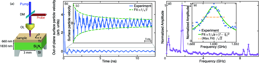
Figure 1: Sample, surface particle velocity variation and acoustic frequency spectrum. (a) Schematic diagram of the sample. DM: dichroic mirror, OL: objective lens. (b) Out-of-plane surface particle velocity measured for co-focused pump and probe beams. (c) Zoom-in of the ZGV Lamb mode amplitude temporal evolution and fit $\propto 1/\sqrt{t}$. (d) Frequency spectrum obtained after a temporal Fourier transform. Arrows indicate the two modes imaged in Fig. 2. (e) Evolution of the normalized amplitude in the frequency window $1.688\leqslant f\leqslant 1.692$ GHz. The solid line is a fit to the experimental data in the form of the square root of a Lorentzian. The dashed line represents $1/\sqrt{2}$ (i.e., -3 dB) of the maximum amplitude of the fit.

In order to facilitate the identification of a ZGV mode, we calculate the acoustic dispersion relation of our bilayer structure, making use of literature elastic constants Briggs (1992) as well as layer thicknesses obtained from ultrafast pulse-echo measurement (see Supplementary Information for details). The first ZGV Lamb mode is predicted to be at frequency $f_{1}^{\rm{th}}=1.7248$ GHz and wavenumber $k_{1}^{\rm{th}}=0.620$ µm^-1. Two other ZGV Lamb modes below 10 GHz are predicted near 3 and 7 GHz (see Table I in the Supplementary Information). We concentrate in this paper on the first ZGV Lamb mode, which has a significant out-of-plane acoustic displacement component.

Detection of a GHz ZGV Lamb mode — Figure 1 shows the temporal evolution of the out-of-plane surface particle velocity for an acoustic frequency of $f=1.6900$ GHz for co-focused pump and probe spots of a few microns in width on the sample (see Methods). This frequency was isolated initially by the help of the above theoretical prediction for the first ZGV resonance and subsequently by frequency tuning. A thermal background variation is subtracted using a polynomial function. This clearly reveals the ZGV resonance, a mode with a lifetime greater than the laser repetition period of $\sim$12 ns (as explained in detail later). An enlarged view of the data is shown in Fig. 1. Two effects contribute to the decay in amplitude. The first originates from the second-order term in the dispersion relation $\omega(k)$ in the vicinity of the ZGV resonance, where $\omega$ is the angular frequency and $k$ the acoustic wavenumber. This produces a $1/\sqrt{t}$ decrease with time $t$, as previously observed at lower frequencies Prada, Clorennec, and Royer (2008a). The second originates from viscoelastic attenuation, yielding a decay $\propto e^{-t/\tau_{0}}$, where $\tau_{0}$ is the mode lifetime, and can be observed only after a certain time has passed. The amplitude decrease in the present case can be fitted to a good approximation with a $1/\sqrt{t}$ function (using least-squares, as with all subsequent fits), as shown in Fig. 1. For our time window equal to $\sim$20 periods of the ZGV mode, no exponential decrease is visible, precluding a derivation of $\tau_{0}$ by this method.

The experimental spectrum obtained from the combination of the different scanned frequencies is displayed in Fig. 1 (see Methods for details). Besides the strong ZGV resonance at 1.6900 GHz, other peaks are observed at 0.2391, 7.2365, 8.3594 and 8.9202 GHz, which are selected a) owing to the choice of pump modulation frequencies, as shown in Methods, b) because with co-focused optical pump and probe spots one only detects modes that do not leave the excitation region, i.e. modes with zero or low group velocity, and c) because with the probe-laser normal incidence only modes with significant normal displacement are detected. The detected modes lie on the $qA_{0}$, $qA_{4}$, $qS_{8}$ and $qS_{5}$ branches of the acoustic dispersion relation, where $qA$ refers to quasi-antisymmetric and $qS$ refers to quasi-symmetric Lamb waves (see Supplementary Information). The observed ZGV mode thus corresponds to the $qS_{1}$ ZGV.

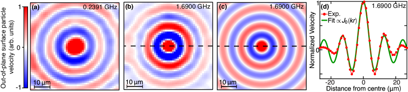
Figure 2: Imaging a ZGV Lamb mode. (a–b) Normalized images of the measured out-of-plane surface particle velocity at (a) 0.2391 and (b) 1.6900 GHz GHz. The $x$ and $y$ axis directions are shown in Fig. 1. Animations are viewable in the Supplementary Information. (c) 2D acoustic field based on a fit to a Bessel function $J_{0}(kr)$. (d) Normalized out-of-plane surface particle velocity evolution of the experimental (dots) and fitted (solid line) data as a function of radial distance (dashed lines in (b)–(c)).

The experimental ($f_{1}^{\rm{exp}}=1.6900$ GHz) and theoretical ($f_{1}^{\rm{th}}=1.7248$ GHz) ZGV frequencies are in reasonable agreement. The residual $\sim$2 % mismatch may be caused either by a difference in the Si₃N₄ layer parameters (see Supplementary Information) or to imperfect adhesion between the two layers Mezil et al. (2014, 2015a). The two other ZGV Lamb modes, predicted near 3 and 7 GHz, could not be detected. This is thought to be owing to a mismatch between the probed frequencies and the ZGV frequencies (see Methods) as well as, for the 7 GHz peak, to the smaller out-of-plane surface displacement expected for this mode (see Supplementary Information).

Figure 1 shows the amplitude-frequency relation around $f_{1}^{\rm{exp}}$. In order to extract the associated Q factor, we fit with the square root of a Lorentzian function, $b/\sqrt{a+(f-f_{0})^{2}}$, where $a,b$ and $f_{0}$ are fitting parameters, yielding $f_{0}=1.6899$ GHz and $Q=1150$. This of the same order of magnitude as the Q factors previously reported for thin composite silicon-nitride/metal/oxide plates suspended by thin beams and driven in thickness longitudinal resonances at similar frequencies Pang et al. (2004). For ZGV modes, Q factors up to 14700 at MHz frequencies have been observed in other materials Clorennec et al. (2006); Prada et al. (2009), values which depend strongly on the ultrasonic attenuation at the frequency in question, as discussed in the next section, as well as parameters such as the possible imperfect adhesion between the two layers.

Imaging a ZGV Lamb mode — The spatiotemporal evolution of the acoustic field is imaged by scanning the probe spot in 2D over a $55\times 55$ µm² area using 301 frames. We specifically target the ZGV mode (at $f_{1}^{\rm{exp}}$) and the branch $qA_{0}$ at $\sim$0.24 GHz, indicated by the two downward pointing arrows in Fig. 1. To eliminate unwanted frequency components, filtering of small and high wavenumbers is conducted in Fourier space. We thereby extract the amplitude field, as shown in Fig. 2 and 2 for $f=0.2391$ and $f_{1}^{\rm{exp}}=1.6900$ GHz, respectively (also viewable as animations in a Multimedia view). The 1.6900 GHz data represents, to our knowledge, the first experimental 2D movie of a ZGV mode, extending the 1D observations of Laurent et al. Laurent, Royer, and Prada (2014). Comparing the animations, one can immediately ascertain that the ZGV mode is not propagating, in striking contrast to the $qA_{0}$ branch, which corresponds to propagating modes.

For a single-frequency point-excited wave in two dimensions, the radial form of the out-of-plane displacement is proportional to $J_{0}(kr)$, where $J_{0}$ is the first-order Bessel function and $r$ is the radial distance (see, e.g., Ref. 28). This has previously been confirmed by theory and by simulation for ZGV Lamb modes Prada, Clorennec, and Royer (2008a); Balogun, Murray, and Prada (2007). Figure 2 shows a fit to our data at 1.6900 GHz with the function $J_{0}(kr$), which gives reasonable agreement, also clear from the cross section shown in Fig. 2. The value of $k$ for the best fit, $k_{1}^{\rm{exp}}=0.55\pm 0.13$ µm^-1, is in fair correspondence with the predicted value $k_{1}^{\rm{th}}=0.620$ µm^-1 from the theoretical dispersion relation . One can notice that the experimental amplitude on the first main side lobes is slightly larger than the theoretical Bessel fitted function, which is in agreement with the results obtained by Laurent et al.Laurent, Royer, and Prada (2014). Away from the central peak, the experimental amplitude is lower; these effects can be attributed to high-frequency material losses.

Our measurement of Q factor ($Q=1150$) and wavenumber ($k_{1}^{\rm{exp}}=0.55$ µm^-1) for the ZGV mode at 1.6900 GHz allows an estimate of the lifetime $\tau_{0}$. As a first step, for a free-standing layer of a single isotropic material and considering only viscoelastic losses Prada, Clorennec, and Royer (2008a); Clorennec et al. (2006), the spatial attenuation coefficient is given by

$$\alpha=\frac{k}{2Q},$$ (1)

where $\alpha$ is an effective attenuation coefficient (in m^-1). This relation yields $\alpha=240$ m^-1 for the above-mentioned ZGV mode. One can then make use of the relation $\tau_{0}$=$1/(\alpha v_{p})$, where $v_{p}$ is the phase velocity to find $\tau_{0}$$\approx$0.22 µs. This is much longer than the time $\sim$10 ns, for an acoustic mode with a typical sound velocity $\sim$5 km/s to leave the imaged region of $55\times 55$ µm² in which the ZGV amplitude is significant.

The value of $\alpha$ obtained can be compared with other high frequency measurements. Assuming an $f^{2}$ variation in $\alpha$, as expected from viscous losses, our value $\alpha=240$ m^-1 lies between those extrapolated for longitudinal waves in silicon nitride (29 m^-1) or polycrystalline titanium (2300 m^-1) to a frequency of 1.69 GHz Mansfeld, Alekseev, and Kotelyansky (2001); Emery and Devos (2006). A detailed comparison is difficult because ZGV modes couple both longitudinal and transverse strain components, which are distributed over the two layers (see Fig. S2 in the Supplementary Information).

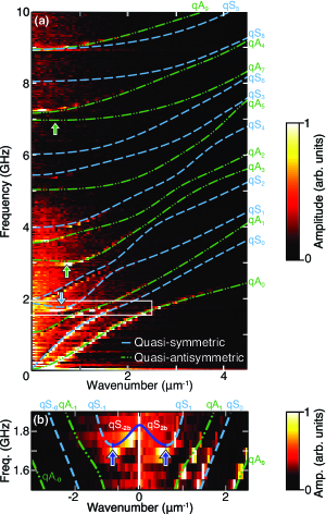
Figure 3: Dispersion curves of the bilayer. (a–b) Experimental (image) and theoretical (dashed and dotted-dashed lines) dispersion curves for (a) $0\leqslant f\leqslant 10$ GHz and $0\leqslant k\leqslant 4.5$ µm^-1 (b) at frequencies near the first ZGV mode for $1.5\leqslant f\leqslant 1.9$ GHz and $-2.5\leqslant k\leqslant 2.5$ µm^-1. The solid navy blue section of the dispersion curves corresponds to the portions where the phase and group velocities are anti-parallel. (a) The box corresponds to the enlarged region in (b) for $k>0$. (a-b) Arrows indicate ZGV points. Plots are independently normalized.

Dispersion curves — More complete information is available with an experimental knowledge of the Lamb-wave dispersion curves. To this end, the pump beam is focused to a micron-sized line source with a cylindrical lens (see Methods). The probe beam spot is scanned along the direction $x$ ($>0$, see Fig. 1) perpendicular to this line source over distances up to 100 µm in 0.05 µm steps to obtain the spatiotemporal variation of the acoustic field. A 2D FT (temporal FT and 1D spatial FT) allows the extraction of the acoustic dispersion curves, as shown in Fig. 3 for both experiment and theory, which show good agreement for the modes visible in experiment (bright regions). The positive wavenumbers in Fig. 3 correspond to waves with phase velocity along the $+x$ direction. The three branches $qA_{0}$, $qS_{0}$ and $qA_{1}$, observed here below $\sim$2 GHz, are detected for a wide range of wavenumbers, unlike branches with higher frequencies, which are detected only for small wavenumbers $k$. The first ZGV mode is clearly observed at $k=0.54\pm$0.03 µm^-1, in agreement with the value extracted in the 2D-scan experiment. The second ZGV mode, predicted at $f_{2}^{\rm{th}}=3.0024$ GHz and $k_{2}^{\rm{th}}=0.732$ µm^-1 is evident at $f_{2}^{\rm{exp}}=2.972$ GHz and $k_{2}^{\rm{exp}}=0.83\pm 0.03$ µm^-1, in fair agreement. This mode may not have been observed in the previous experiment with co-focused laser beams owing to the different excited wave vector spectrum ($k_{1}^{th}<k_{2}^{th}$). Other peaks that were previously detected at 0.2391, 7.2365 and 8.9202 GHz are again evident on the branches $qA_{0}$, $qA_{4}$ and $qS_{5}$, respectively. (The mode previously detected at 8.3594 MHz is absent here, and no corresponding mode appears on the dispersion relation. Its previous appearance in the spectrum of Fig. 1 seems likely to be an experimental artifact.) Some branches, such as $qA_{2}$ near $3.6$ GHz as well as $qS_{0}$ and $qA_{1}$, are revealed only in this new measurement. We attribute residual discrepancies between the theoretical and experimental dispersion curves to uncertainties in the elastic parameters and in the layer thicknesses, and to the possible imperfect layer bonding Vlasie and Rousseau (2003).

The dispersion curves in Fig. 3 are a magnified view of Fig. 3, this time including negative wavenumbers corresponding to $-x$-directed propagation. The main features are as follows:

1. for the $qA_{0}$, $qS_{0}$ and $qA_{1}$ branches and the region $(\omega,k)$ with $|k|$ larger than that for the $qS_{1}$ ZGV (the latter indicated by a downward-pointing arrow in Fig. 3), the intensity is much greater for $k>0$;

2. for the region $(\omega,k)$ with $|k|$ smaller than that for the $qS_{1}$ ZGV, the intensity is much greater for $k<0$;

3. for the region $(\omega,k)$ in the vicinity of the $qS_{1}$ ZGV, near wavenumber $k_{1}$ and frequency $f_{1}$, the intensities for $k>0$ and $k<0$ are comparable.

Discussion

Because of the symmetry of the excitation with respect to coordinate $x$, acoustic waves with positive and negative $k$ should be generated with equal amplitude and initially form a single wave packet located at the excitation point. This wave packet is eventually broadened and split because of the acoustic dispersion and the broad distribution of positive and negative values of $k$. Its wave components are plane-wave modes spreading over all 2D space, but in general, their sum is observable as a wave packet only if their phase constructively interferes. In other words, there are two possibilities for observing no acoustic field: a complete lack of such modes or the overlapping of several modes with random phase. (Compare the Fourier transform of a $\delta$-function: it contains an infinite number of fully spreading plane waves, but is only finite at a point in space.) Since we observe the waves in the region $x>0$, the waves we can primarily observe are restricted to those with $v_{g}\geqslant 0$. Waves with $v_{g}<0$ exist, but give negligible contribution to the waves we observe because we only probe for positive $x$ values over a region with little overlap with the pump spot.

The feature 1) above can therefore be attributed to the waves having co-directed group velocity $v_{g}$ and phase velocity $v_{p}$. With reference to the dispersion curves, all $k$ values involved in feature 1) show positive group velocity $v_{g}>0$. On the other hand, feature 2) can be attributed to the waves having anti-parallel $v_{g}$ and $v_{p}$; the $k$ values involved in feature 2) can be seen to be negative, but are associated with a positive slope on the $\omega$-$k$ plot, i.e., they possess $v_{g}>0$ but with $v_{p}<0$. The feature 3) can be attributed to the waves with zero or very small group velocity. The wave packet consisting of these near-zero or zero-$v_{g}$ wave components remains almost stationary, and both positive and negative $k$ components contribute to this wave packet over an extended period of time. These features are consistent with those of Philippe et al. Philippe, Murray, and Prada (2015). In Fig. 3 we label the part of the +$k$ $qS_{1}$ branch with the negative slope as $qS_{2b}$ (and $qS_{-2b}$ for the equivalent $-k$ part), in agreement with standard nomenclature Meitzler (1965); Prada, Clorennec, and Royer (2008b), where $b$ stands for ‘backward wave’. All other branches with finite positive group velocity are observed only for $k>0$, with the exception of $qS_{5}$ near 9 GHz, for which $v_{g}$ is small for low $k$, and this branch is observed for both positive and negative $k$ with similar amplitude. Only the branch containing the ZGV point at 1.6900 GHz has a greater amplitude for negative $k$ compared with that for positive $k$.

In conclusion, we image a zero-group-velocity Lamb mode in two dimensions. We apply an ultrafast time-domain technique with arbitrary GHz-acoustic frequency control to a nanoscale bilayer consisting of a silicon-nitride plate coated with a titanium film to provide this observation at unprecedented frequencies in the GHz range. Our combination of both time-domain 1D and 2D optical scanning methods provides a comprehensive probe for the ZGV dynamics. We isolate the $qS$₁ ZGV mode at $\sim$1.7 GHz and probe its spatial and temporal characteristics, including its Q factor $\sim$1000. The spatial form of this quasi-point-excited ZGV is directly verified by Fourier analysis to correspond closely to the expected Bessel function in 2D, allowing its wavenumber to be derived and its ZGV nature to be directly verified in the time domain from its relatively long lifetime $\sim$0.2 µs. Experimental dispersion curves of this bilayer system are also obtained, and show good agreement with a theoretical model and reveal other ZGV modes.

Applications of real-time imaging of ZGV Lamb modes include detecting defects in adhesion and deviations in interfacial stiffnesses, so this high frequency imaging technique should provide new avenues for evaluating and quantifying the mechanical integrity of nanostructures.

Methods

Measurement setup — A Ti:sapphire pulsed laser produces a series of $\sim$100 fs width pulses at repetition rate $f_{\text{rep}}=80.38$ MHz and wavelength 830 nm. Part of this beam is frequency doubled ($\lambda=415$ nm) and used for the pump with a pulse energy of $\sim$0.15 nJ. It is intensity modulated with an acousto-optic modulator (AOM) at frequency $f_{p}$. For experiments with a circular pump spot, the pump beam is focused on the Ti film side of the sample at normal incidence with a $\times 50$ objective lens to a 4.2 µm radius (at $1/e^{2}$ intensity) to optimize the first ZGV Lamb mode generation (see Supplementary Information). This generates, in the centre of the pump spot, an instantaneous temperature rise of $\sim$80 K after each laser pulse and a steady state temperature rise of $\sim$50 K . The Lamb waves thermoelastically generated with our pump are calculated to have an amplitude of $\sim$10 pm. To determine the dispersion relation experiments are also carried out using a pump spot in the form of a line of 1/$e^{2}$ intensity full-width 1.5 µm and a length of 5 µm.

The other part of the beam, at $\lambda=830$ nm, is used for the probe. It is focused to a 2.8 µm radius (at $1/e^{2}$ intensity) for both types of pump beam focusing with the same objective lens as used for the pump and with a $\sim$0.03 nJ pulse energy. When required, it is intensity modulated with another AOM at the frequency $f_{s}$. The modulation frequency is set to allow heterodyne detection within the 3 MHz photodetector bandwidth ($|f_{p}-f_{s}|\leqslant 3$ MHz). A Sagnac interferometer is incorporated Tachizaki et al. (2006), producing two probe pulses separated by a time interval of $t<200$ ps. A delay line and a 2D spatial scanning system making use of a two-axis displacement stage with a lens pair are mounted in the path of the probe beam to access the spatiotemporal evolution of the acoustic field at the sample surface at 20 Hz bandwidth. The out-of-plane surface particle velocity modulates the optical phase, which is converted to an intensity modulation that is detected with a lock-in amplifier. The arbitrary-frequency technique allows one to access frequencies $nf_{\text{rep}}+mf_{p}$, $n$ an integer and $m=\pm 1$, by recording both in-phase and quadrature components Matsuda et al. (2015); Kaneko, Matsuda, and Tomoda (2014); Mezil et al. (2015b).

Data analysis — The setup used here makes use of the following: double modulation (i.e. intensity modulation of both pump and probe beams), a delay set in the probe-beam line, and a probe modulation upstream of the delay. The arrangement is described in detail in Ref. 21. Because of the pump intensity modulation, the excited frequencies are $nf_{\text{rep}}+mf_{p}$, where $m=+1$ for the upper sideband and $-1$ for the lower sideband. The generated acoustic field can be expressed as a superposition of these frequency components as

$$S(t)=\sum_{n,m}A_{n,m}\cos[-(n\omega_{\text{rep}}+m\omega_{p})t+\phi_{n,m}],$$ (2)

where $A_{n,m}$ and $\phi_{n,m}$ are the position dependent amplitude and phase of a vibrational mode $(n,m)$ of frequency $nf_{\text{rep}}+mf_{p}$. In the summation of Eq. 2, the case $(n,m)=(0,-1)$ is not included. From the detection system (i.e. a photodetector connected to a lock-in amplifier), we access the in-phase ($X$) and quadrature ($Y$) components of the lock-in output, which are proportional to the acoustic out-of-plane surface particle velocity. Both are functions of delay time $\tau$ and probe spot position. The complex signal $Z\equiv X+iY\text{sgn}(\omega_{p}-\omega_{s})$ can be rewritten as

$$Z(\tau)=\sum_{n,m}A_{n,m}e^{im[-(n\omega_{\text{rep}}+m\omega_{s})\tau+\phi_{n,m}]}.$$ (3)

In the summation of Eq. 3, again the case $(n,m)=(0,-1)$ is not included. The amplitude and the phase are found from a Fourier transform (FT):

$$A_{n,m}e^{im\phi_{n,m}}=\frac{1}{T}\int^{T}_{0}Z(\tau)e^{i(mn\omega_{\text{rep}}+\omega_{s})\tau}d\tau.$$ (4)

It is then possible to analyze the data at an angular frequency $\omega$ as a real-valued term involved in Eq. 2, i.e., giving a spatial pattern of the vibration at $\omega=2\pi(nf_{\text{rep}}+mf_{p})$. Modifying the frequency $f_{p}$ thus allows arbitrary acoustic frequency control.

In the first experiment, the pump frequency $f_{p}$ is increased from 0.1 up to 4 MHz by steps of 0.1 MHz. This provides data at frequencies $nf_{\text{rep}}+mf_{p}$. In the spectrum displayed in Fig. 1, one can see the amplitude evolution associated with $n=21$ and $m=+1$ for all these pump frequencies. The maximum amplitude is obtained for $f_{p}=2.0$ MHz. In the following experiments the pump frequency is maintained at $f_{p}=2.0$ MHz to optimize the ZGV Lamb mode generation. The resulting measured acoustic frequencies are $nf_{\text{rep}}\pm 2.0$ MHz. In Fig. 1 the analysis covers all the scanned frequencies, but for each $n$ only the maximum amplitude is displayed for clarity (e.g., for $n=21$ only the point associated with $f_{p}=2.0$ MHz is displayed).

References

Author contributions

O.B.W. and S.M. proposed the research goals and supervised the project. Q.X. performed experiments with the help of S.M. and M.T. The theoretical model and numerical model was developed by S.M. and J.L. Data was analyzed by Q.X., S.M. and P.H.O. Theoretical support was provided by S.M., O.M., Z.S. and O.B.W. All authors helped prepare, critically review and revise the manuscript.

Additional information

Supplementary Information accompanies this paper.
Multimedia animations are available at this link.
Competing interests: The authors declare no competing interests.

References

- Ranka, Windeler, and Stentz (2000) J. K. Ranka, R. S. Windeler, and A. J. Stentz, “Visible continuum generation in air–silica microstructure optical fibers with anomalous dispersion at 800 nm,” Opt. Lett. 25, 25–27 (2000).
- Laurent et al. (2015) J. Laurent, D. Royer, T. Hussain, F. Ahmad, and C. Prada, “Laser induced zero-group velocity resonances in transversely isotropic cylinder,” J. Acoust. Soc. Am. 6, 3325–3334 (2015).
- Holland and Chimenti (2003) S. D. Holland and D. E. Chimenti, “Air-coupled acoustic imaging with zero-group-velocity Lamb modes,” Appl. Phys. Lett. 83, 2704–2706 (2003).
- Prada, Balogun, and Murray (2005) C. Prada, O. Balogun, and T. W. Murray, “Laser-based ultrasonic generation and detection of zero-group velocity Lamb waves in thin plates,” Appl. Phys. Lett. 87, 194109 (2005).
- Milián and Skryabin (2014) C. Milián and D. V. Skryabin, “Soliton families and resonant radiation in a micro-ring resonator near zero group-velocity dispersion,” Opt. Express 22, 3732–3739 (2014).
- Ibanescu et al. (2005) M. Ibanescu, S. G. Johnson, D. Roundy, Y. Fink, and J. D. Joannopoulos, “Microcavity confinement based on an anomalous zero group-velocity waveguide mode,” Opt. Lett. 30, 552–554 (2005).
- Rayleigh (1889) L. Rayleigh, “On the free vibrations of an infinite plate of homogeneous isotropic elastic matter,” Proc. London Math. Society 20, 225—234 (1889).
- Clorennec, Prada, and Royer (2007) D. Clorennec, C. Prada, and D. Royer, “Local and noncontact measurements of bulk acoustic wave velocities in thin isotropic plates and shells using zero group velocity Lamb modes,” J. Appl. Phys. 101, 034908 (2007).
- Cès et al. (2011) M. Cès, D. Clorennec, D. Royer, and C. Prada, “Thin layer thickness measurements by zero group velocity Lamb mode resonances,” Rev. Sci. Instrum. 82, 114902 (2011).
- Cès, Royer, and Prada (2012) M. Cès, D. Royer, and C. Prada, “Characterization of mechanical properties of a hollow cylinder with zero group velocity Lamb modes,” J. Acoust. Soc. Am. 132, 180–185 (2012).
- Grünsteidl et al. (2016) C. Grünsteidl, T. W. Murray, T. Berer, and I. A. Veres, “Inverse characterization of plates using zero group velocity Lamb modes,” Ultrasonics 65, 1–4 (2016).
- Mezil et al. (2014) S. Mezil, J. Laurent, D. Royer, and C. Prada, “Non contact probing of interfacial stiffnesses between two plates by zero-group velocity Lamb modes,” Appl. Phys. Lett. 105, 021605 (2014).
- Mezil et al. (2015a) S. Mezil, F. Bruno, S. Raetz, J. Laurent, D. Royer, and C. Prada, “Investigation of interfacial stiffnesses of a tri-layer using zero-group velocity Lamb modes,” J. Acoust. Soc. Am. 138, 3202–3209 (2015a).
- Yan et al. (2018) G. Yan, S. Raetz, N. Chigarev, V. E. Gusev, and V. Tournat, “Characterization of progressive fatigue damage in solid plates by laser ultrasonic monitoring of zero-group-velocity Lamb modes,” Phys. Rev. Appl. 9, 061001 (2018).
- Dixon, Edwards, and Palmer (2001) S. Dixon, C. Edwards, and S. B. Palmer, “High accuracy non-contact ultrasonic thickness gauging of aluminium sheet using electromagnetic acoustic transducers,” Ultrasonics 39, 445–453 (2001).
- Yantchev et al. (2011) V. Yantchev, L. Arapan, I. Katardjiev, and V. Plessky, “Thin-film zero-group-velocity lamb wave resonator,” Appl. Phys. Lett. 99 (2011).
- Balogun, Murray, and Prada (2007) O. Balogun, T. W. Murray, and C. Prada, “Simulation and measurement of the optical excitation of the S1 zero group velocity Lamb wave resonance in plates,” J. Appl. Phys. 102, 064914 (2007).
- Clorennec et al. (2006) D. Clorennec, C. Prada, D. Royer, and T. W. Murray, “Laser impulse generation and interferometer detection of zero group velocity Lamb mode resonance,” Appl. Phys. Lett. 89, 024101 (2006).
- Tomoda et al. (2014) M. Tomoda, S. Matsueda, P. H. Otsuka, O. Matsuda, I. A. Veres, V. E. Gusev, and O. B. Wright, “Imaging acoustic waves in microscopic wedges,” New J. Phys. 16 (2014).
- Kaneko, Matsuda, and Tomoda (2014) S. Kaneko, O. Matsuda, and M. Tomoda, “A method for the frequency control in time-resolved two-dimensional gigahertz surface acoustic wave imaging,” AIP adv. 4, 017142 (2014).
- Matsuda et al. (2015) O. Matsuda, S. Kaneko, O. B. Wright, and M. Tomoda, “Time-resolved gigahertz acoustic wave imaging at arbitrary frequencies,” IEEE Trans. Ultrason., Ferroelectr. Freq. Control 62, 584–595 (2015).
- Tachizaki et al. (2006) T. Tachizaki, T. Muroya, O. Matsuda, Y. Sugawara, D. H. Hurley, and O. B. Wright, “Scanning ultrafast sagnac interferometry for imaging two-dimensional surface wave propagation,” Rev. Sci. Instrum. 77, 043713 (2006).
- Briggs (1992) A. Briggs, Acoustic Microscopy, pp 102-103 (Clarendon, Oxford, 1992).
- Prada, Clorennec, and Royer (2008a) C. Prada, D. Clorennec, and D. Royer, “Power law decay of zero group velocity Lamb modes,” Wave Motion 45, 723–728 (2008a).
- Pang et al. (2004) W. Pang, H. Zhang, S. Whangbo, and E. S. Kim, “High Q film bulk acoustic resonator from 2.4 to 5.1 GHz,” in 17th IEEE International Conference on Micro Electro Mechanical Systems, Maastricht MEMS 2004 Technical Digest (IEEE, 2004) pp. 805–808.
- Prada et al. (2009) C. Prada, D. Clorennec, T. W. Murray, and D. Royer, “Influence of the anisotropy on zero-group velocity Lamb modes,” J. Acoust. Soc. Am. 126, 620–625 (2009).
- Laurent, Royer, and Prada (2014) J. Laurent, D. Royer, and C. Prada, “Temporal behavior of laser induced elastic plate resonances,” Wave Motion 51, 1011–1020 (2014).
- Wright et al. (2002) O. B. Wright, Y. Sugawara, O. Matsuda, M. Takigahira, Y. Tanaka, S. Tamura, and V. E. Gusev, “Real-time imaging and dispersion of surface phonons in isotropic and anisotropic materials,” Physica B: Condensed Matter 316-317, 29–34 (2002).
- Note (1) The fit does not take into account the smoothing due to the finite spot diameters, but we verified that its effect has a negligible influence on the fitted curve.
- Mansfeld, Alekseev, and Kotelyansky (2001) G. Mansfeld, S. Alekseev, and I. Kotelyansky, “Acoustic HBAR spectroscopy of metal (W, Ti, Mo, Al) thin films,” in Ultrasonics Symposium, 2001 IEEE, Vol. 1 (IEEE, 2001) pp. 415–418.
- Emery and Devos (2006) P. Emery and A. Devos, “Acoustic attenuation measurements in transparent materials in the hypersonic range by picosecond ultrasonics,” Appl. Phys. Lett. 89, 191904 (2006).
- Vlasie and Rousseau (2003) V. Vlasie and M. Rousseau, “Acoustical validation of the rheological models for a structural bond,” Wave Motion 37, 333–349 (2003).
- Philippe, Murray, and Prada (2015) F. D. Philippe, T. W. Murray, and C. Prada, “Focusing on plates: controlling guided waves using negative refraction,” Sci. Rep. 5, 11112 (2015).
- Meitzler (1965) A. H. Meitzler, “Backward-wave transmission of stress pulses in elastic cylinders and plates,” J. Acoust. Soc. Am. 38, 835–842 (1965).
- Prada, Clorennec, and Royer (2008b) C. Prada, D. Clorennec, and D. Royer, “Local vibration of an elastic plate and zero-group velocity Lamb modes,” J. Acoust. Soc. Am. 124, 203–212 (2008b).
- Note (2) The steady state temperature rise of the sample at the centre of the optical pump spot is estimated by considering a finite-sized effectively 2D circular plate and approximating the laser intensity profile to a top hat distribution. Under such assumptions, the solution of the heat diffusion equation gives , where is the power absorbed by the sample ( with mW the measured incident power before the objective lens, =0.83 the optical transmittance of the objective lens at 415 nm—the pump wavelength—and =0.444 the optical reflection coefficient of Ti at 415 nm), the bilayer thickness (with , nm), W/m.K the thermal conductivity estimated by weighting the values for each layer by their thickness (, W/m.K), mm the plate radius (the circular plate being chosen to have the same area as the square sample plate surface mm2) and µm the intensity radius of the pump beam. Reflection coefficients and thermal conductivities are taken from Ref. 39.
- Mezil et al. (2015b) S. Mezil, P. H. Otsuka, S. Kaneko, O. B. Wright, M. Tomoda, and O. Matsuda, “Imaging arbitrary acoustic whispering-gallery modes in the gigahertz range with ultrashort light pulses,” Opt. Lett. 40, 2157–2160 (2015b).
- Note (3) We assume and where is the signal from the photodetector and .
- Lide (2010) D. R. Lide, CRC Handbook of Chemistry and Physics (CRC-Press, 2010).
Acknowledgements
The authors are grateful to Claire Prada and Alex Maznev for fruitful discussions. S. Mezil carried out this work as an International Research Fellow of the Japanese Society for the Promotion of Science (JSPS).