Invariant, Viability and Discriminating Kernel Under-Approximation via Zonotope Scaling

Abstract.

Scalable safety verification of continuous state dynamic systems has been demonstrated through both reachability and viability analyses using parametric set representations; however, these two analyses are not interchangable in practice for such parametric representations. In this paper we consider viability analysis for discrete time affine dynamic systems with adversarial inputs. Given a set of state and input constraints, and treating the inputs in best-case and/or worst-case fashion, we construct invariant, viable and discriminating sets, which must therefore under-approximate the invariant, viable and discriminating kernels respectively. The sets are constructed by scaling zonotopes represented in center-generator form. The scale factors are found through efficient convex optimizations. The results are demonstrated on two toy examples and a six dimensional nonlinear longitudinal model of a quadrotor.

1. Introduction

Reachability analysis is a rigorous alternative to sampling-based verification of dynamic systems, and at least for linear (or affine) systems there have been recent demonstrations of techniques capable of handling thousands of continuous state space dimensions (Bak and Duggirala, 2017; Bogomolov et al., 2018). Reachable sets and tubes—or more typically over-approximations of them to ensure soundness—are an effective tool for demonstrating safety: If the forward / backward reach set or tube does not intersect the unsafe / initial set respectively then the system is safe. Any input or parameter uncertainty is typically treated in a worst-case fashion to make the reach set or tube larger and hence the system less likely to be judged safe.

In this paper we adopt the alternative approach to proving safety advocated in viability theory (Aubin et al., 2011) but more commonly framed as various versions of invariant sets: Find the set of states from which trajectories of the system are guaranteed to satisfy a specified safety constraint. A critical feature of viable or controlled invariant sets is that a control input may be chosen in a best-case fashion to keep the trajectories safe. Robust versions of these sets (aka discriminating sets) also allow an adversarial disturbance input which is treated in a worst-case fashion to drive the trajectories out of the safety constraints. In every case we must under-approximate the results to ensure soundness of the safety analysis.

While viability analysis can be reduced to reachability analysis and vice versa in theory, the parametric representations which can handle high dimensional systems do not support such reductions; for example, the reductions require set complements but the parametric representations are usually restricted to convex sets whose complements are non-convex.

The need to develop scalable algorithms for viability / invariance in addition to those for reachability is therefore practical: The former require under-approximation while the latter over-approximation, and some analyses are more naturally amenable to parametric representations in one formulation or the other, but rarely both. Although we do not have space to explore it in this paper, an example of an application which naturally fits into the viability framework is testing at run-time whether an exogenous input signal—such as might arise from a human-in-the-loop control—will maintain safety; for example, see (Mitchell et al., 2016).

The focus of this paper is therefore development of more scalable formulations for (robust) invariance / viability based analysis of affine continuous state dynamic systems. Scalability is achieved by framing the calculations as convex optimizations to find efficient parametric representations in the form of zonotopes. The specific contributions of this paper are to:

• Show how a finite horizon invariance kernel of an affine system with disturbance input can be underapproximated with a zonotope via a linear program.

• Extend the formulation to allow control inputs and thereby underapproximate finite horizon viability and discriminating kernels with zonotopes via a convex program.

• Demonstrate the use of the discriminating kernel to compute a larger robust controlled invariant set for a moderate dimensional nonlinear quadrotor model than was achieved using an ellipsoidal representation in (Mitchell et al., 2016).

2. Related Work

Reachability and viability have been applied to a broad variety of different dynamic systems resulting in a huge range of different algorithms. We focus here on parametric approaches for linear or affine dynamics. Ellipsoid and support vector parametric representations of viability constructs were explored in (Maidens et al., 2013; Mitchell and Kaynama, 2015). Zonotopic representations for reachability were introduced in (Girard, 2005) and have since been extensively explored; for example (Girard et al., 2006; Althoff and Krogh, 2011; Althoff and Frehse, 2016). Our work was inspired, however, by the papers (Schürmann and Althoff, 2017a, c) and in particular (Schürmann and Althoff, 2017b), which utilizes a convex optimization to select zonotope generator weights to construct a control scheme that will drive a set of initial states into the smallest possible set of final states. Also similar to this work is (Han et al., 2016) in which the authors seek a linear feedback control input which will maximize the size of the backward reachable set and arrive at a bilinear matrix inequality based on containment of one zonotope within another. Significantly, unlike most other work these papers treat the input in a best-case fashion. The difference with the work below lies in the reachability vs viability formulation and the fact that our approach constructs a set-valued viable feedback control from a convex optimization.

3. Preliminaries

For a matrix $\mathrm{M}$, let $|\mathrm{M}|$ denote the elementwise absolute value and $({\mathrm{M}})_{i,j}$ denote the element in row $i$ and column $j$; therefore, $({\mathrm{M}^{s}})_{i,j}$ denotes the element in row $i$ and column $j$ of the matrix power $\mathrm{M}^{s}$. Also define $\mathbf{1}_{d}$ and $\mathbf{0}_{d}$ to be the vectors in $\mathbb{R}^{d}$ of all ones and all zeros respectively.

3.1. System Dynamics

Consider a discrete time dynamic system for times $t=0,1,2,\ldots$:

(1) $$x(t+1)=\mathrm{A}x(t)+\mathrm{B}u(t)+\mathrm{C}v(t)+w$$

where

• The state is $x\in\mathbb{R}^{d_{x}}$.

• The control input is $u\in\mathcal{U}\subset\mathbb{R}^{d_{u}}$. The control input constraint $\mathcal{U}$ is an interval hull (or hyperrectangle) defined by the elementwise inequalities

  (2) $$\mathcal{U}=\{u\in\mathbb{R}^{d_{u}}\mid\underline{u}\leq u\leq\overline{u}\}.$$

• The disturbance input is $v\in\mathcal{V}\subset\mathbb{R}^{d_{v}}$. The disturbance input constraint $\mathcal{V}$ is a zonotope (see section 3.3).

• The drift $w\in\mathbb{R}^{d_{x}}$ is constant. We note that $w\neq 0$ can alternatively be treated by offsetting the center of the zonotope $\mathcal{V}$, but we will carry $w$ through separately so as to support a drift term for disturbance-free systems.

Given an initial condition $x(0)$ and input signals $u(\cdot)$ and $v(\cdot)$, the solution of (1) is given by

(3) $$x(t)=\mathrm{A}^{t}x(0)+\sum_{s=0}^{t-1}\mathrm{A}^{t-1-s}\left(\mathrm{B}u(s)+\mathrm{C}v(s)+w\right).$$

3.2. Sets of Interest for Safety Verification

We will formulate our safety verification problem as keeping the system state within a constraint set $\mathcal{X}$. For reasons of notational simplicity, we will assume in the rest of the paper that $\mathcal{X}$ is an interval hull or box constraint of the form

(4) $$\mathcal{X}=\{x\in\mathbb{R}^{d_{x}}\mid\underline{x}\leq x\leq\overline{x}\}.$$

It is possible to relax this assumption; see section 7 for further comments.

We seek to approximate various subsets of the constraint set. The most general is a finite horizon discriminating or robust controlled invariant set

(5) $$\mathsf{Disc}\left({[0,T]},{\mathcal{X}}\right)\triangleq\left\{x(0)\in\mathcal{X}\,\left|\,\begin{gathered}\exists u(\cdot),\forall v(\cdot),\forall t\in[0,T],\\ x(t)\in\mathcal{X}\end{gathered}\right.\right\},$$

where $u(t)\in\mathcal{U}$ and $v(t)\in\mathcal{V}$ for all $t=0,\ldots,T$. Note that the control input $u(t)$ tries to keep the system state within the constraint set $\mathcal{X}$, while the disturbance input $v(t)$ is treated in a worst-case or adversarial fashion and tries to drive the system state outside the constraint set.

We will also consider two special cases of the discriminating set. For systems which lack a control input, we seek a finite horizon invariant set

(6) $$\mathsf{Inv}\left({[0,T]},{\mathcal{X}}\right)\triangleq\left\{x(0)\in\mathcal{X}\,\left|\,\begin{gathered}\forall v(\cdot),\forall t\in[0,T],\\ x(t)\in\mathcal{X}\end{gathered}\right.\right\},$$

while for systems which lack a disturbance input we seek a finite horizon viable or controlled invariant set

(7) $$\mathsf{Viab}\left({[0,T]},{\mathcal{X}}\right)\triangleq\left\{x(0)\in\mathcal{X}\,\left|\,\begin{gathered}\exists u(\cdot),\forall t\in[0,T],\\ x(t)\in\mathcal{X}\end{gathered}\right.\right\}.$$

Our algorithm for computing these previous sets will often make use of the forward reach set of some specified set $\mathcal{S}$.

(8) $$\mathsf{R}\left({t},{\mathcal{S}}\right)\triangleq\left\{x(t)\in\mathbb{R}^{d_{x}}\,\left|\,\exists w(\cdot),x(0)\in\mathcal{S}\right.\right\},$$

where the choice of input signal $w(\cdot)=u(\cdot)$ or $w(\cdot)=v(\cdot)$ should be clear from context. Unlike the discriminating, invariant and viable sets, the reach set is defined at a single time rather than over an interval, and the set $\mathcal{S}$ is an initial condition rather than a constraint.

3.3. Set Representation: Zonotopes

We will use zonotopes as our parametric representation of invariant, viable and/or discriminating sets. A zonotope $\mathcal{S}\subseteq\mathbb{R}^{d}$ is a polytope defined by a center ${c}\left({\mathcal{S}}\right)\in\mathbb{R}^{d}$ and a finite number of generators ${g}_{i}\left({\mathcal{S}}\right)\in\mathbb{R}^{d}$ for $i=1,\ldots,p\left({\mathcal{S}}\right)$:

(9) $$\mathcal{S}=\left\{\left.{c}\left({\mathcal{S}}\right)+\sum_{i=1}^{p\left({\mathcal{S}}\right)}\lambda_{i}{g}_{i}\left({\mathcal{S}}\right)\;\right|\;{-1}\leq\lambda_{i}\leq+1\right\}.$$

In most cases it is more convenient to work with the center-generator tuple (or G-representation for a zonotope $\mathcal{S}$ rather than (9)

$$\mathcal{S} =\langle{c}\left({\mathcal{S}}\right)\mid{g}_{1}\left({\mathcal{S}}\right),{g}_{2}\left({\mathcal{S}}\right),\ldots,{g}_{p\left({\mathcal{S}}\right)}\left({\mathcal{S}}\right)\rangle,$$

$$=\langle{c}\left({\mathcal{S}}\right)\mid\mathrm{G}\left({\mathcal{S}}\right)\rangle,$$

where the generator matrix $\mathrm{G}\left({\mathcal{S}}\right)$ is formed by horizontal concatenation of the generator vectors

$$\mathrm{G}\left({\mathcal{S}}\right)=\begin{bmatrix}{g}_{1}\left({\mathcal{S}}\right)&{g}_{2}\left({\mathcal{S}}\right)&\cdots&{g}_{p\left({\mathcal{S}}\right)}\left({\mathcal{S}}\right)\end{bmatrix}\in\mathbb{R}^{d\times p\left({\mathcal{S}}\right)}.$$

When it is necessary to refer to individual elements of a generator matrix or vector, we will use the notation ${g}_{j,i}\left({\mathcal{S}}\right)$ to specify the element in the $j^{th}$ row and $i^{th}$ column of matrix $\mathrm{G}\left({\mathcal{S}}\right)$, or equivalently the $j^{th}$ element of vector ${g}_{i}\left({\mathcal{S}}\right)$.

With the generator matrix notation, we can write (9) more compactly as

(10) $$\mathcal{S}=\left\{{c}\left({\mathcal{S}}\right)+\mathrm{G}\left({\mathcal{S}}\right)\lambda\;\left|\;{-\mathbf{1}_{p\left({\mathcal{S}}\right)}}\leq\lambda\leq+\mathbf{1}_{p\left({\mathcal{S}}\right)}\right.\right\}.$$

For a vector $x\in\mathcal{S}$, define $\lambda(x,\mathcal{S})$ such that

(11) $$x={c}\left({\mathcal{S}}\right)+\mathrm{G}\left({\mathcal{S}}\right)\lambda(x,\mathcal{S})\text{ and }{-\mathbf{1}_{p\left({\mathcal{S}}\right)}}\leq\lambda(x,\mathcal{S})\leq+\mathbf{1}_{p\left({\mathcal{S}}\right)}$$

and note that by (10) $\lambda(x,\mathcal{S})$ exists but is not necessarily unique.

The coordinate bounds for a zonotope (or equivalently the interval hull containing that zonotope) are easily computed; for example, see (Girard et al., 2006; Althoff and Krogh, 2011). In particular, for $x\in\mathcal{S}$,

(12) $${c}_{j}\left({\mathcal{S}}\right)-\sum_{i=0}^{p\left({\mathcal{S}}\right)}\left|{g}_{j,i}\left({\mathcal{S}}\right)\right|\leq x_{j}\leq{c}_{j}\left({\mathcal{S}}\right)+\sum_{i=0}^{p\left({\mathcal{S}}\right)}\left|{g}_{j,i}\left({\mathcal{S}}\right)\right|,$$

for all $j=1,\ldots,d$, which we can write in compact form as

(13) $${c}\left({\mathcal{S}}\right)-|\mathrm{G}\left({\mathcal{S}}\right)|\mathbf{1}_{p\left({\mathcal{S}}\right)}\leq x\leq{c}\left({\mathcal{S}}\right)+|\mathrm{G}\left({\mathcal{S}}\right)|\mathbf{1}_{p\left({\mathcal{S}}\right)}.$$

Lemma 3.1.

Consider an interval hull

$$\mathcal{B}=\{b\in\mathbb{R}^{d}\mid\underline{b}\leq b\leq\overline{b}\}.$$

For zonotope $\mathcal{S}\subset\mathbb{R}^{d}$, the containment $\mathcal{S}\subseteq\mathcal{B}$ is equivalent to the constraints

(14) $${c}_{j}\left({\mathcal{S}}\right)-\sum_{i=0}^{p\left({\mathcal{S}}\right)}\left|{g}_{j,i}\left({\mathcal{S}}\right)\right| \geq\underline{b}_{j},$$

$${c}_{j}\left({\mathcal{S}}\right)+\sum_{i=0}^{p\left({\mathcal{S}}\right)}\left|{g}_{j,i}\left({\mathcal{S}}\right)\right|, \leq\overline{b}_{j}$$

for all $j=1,\ldots,d$. More compactly,

(15) $${c}\left({\mathcal{S}}\right)-|\mathrm{G}\left({\mathcal{S}}\right)|\mathbf{1}_{p\left({\mathcal{S}}\right)} \geq\underline{b},$$

$${c}\left({\mathcal{S}}\right)+|\mathrm{G}\left({\mathcal{S}}\right)|\mathbf{1}_{p\left({\mathcal{S}}\right)} \geq\overline{b}.$$

Proof.

A straightforward consequence of the bounds (12) and (13). ∎

The class of zonotopes is closed under linear transformation (Girard, 2005), and the effect of a linear transform on a zonotope is easily implemented using the center-generator tuple representation

$$\mathrm{M}\mathcal{S}=\langle\mathrm{M}{c}\left({\mathcal{S}}\right)\mid\mathrm{M}\mathrm{G}\left({\mathcal{S}}\right)\rangle,\\$$

where $\mathcal{S}$ is a zonotope in dimension $d$ and $\mathrm{M}\in\mathbb{R}^{m\times d}$ is the matrix representing the linear transformation.

Proposition 3.2.

For systems without control inputs but with disturbance inputs constrained by the zonotope

$$\mathcal{V}=\langle{c}\left({\mathcal{V}}\right)|\mathrm{G}\left({\mathcal{V}}\right)\rangle,$$

the center, generator count and generator matrix of the exact reach set $\mathsf{R}\left({t},{\mathcal{S}}\right)$ are

(16) $${c}\left({\mathsf{R}\left({t},{\mathcal{S}}\right)}\right) =\mathrm{A}^{t}{c}\left({\mathcal{S}}\right)+\sum_{s=0}^{t-1}\mathrm{A}^{t-1-s}\left(\mathrm{C}{c}\left({\mathcal{V}}\right)+w\right),$$

$$p\left({\mathsf{R}\left({t},{\mathcal{S}}\right)}\right) =p\left({\mathcal{S}}\right)+tp\left({\mathcal{V}}\right),$$

$$\mathrm{G}\left({\mathsf{R}\left({t},{\mathcal{S}}\right)}\right) =\begin{bmatrix}\mathrm{A}^{t}\mathrm{G}\left({\mathcal{S}}\right)&\mathrm{A}^{t-1}\mathrm{C}\mathrm{G}\left({\mathcal{V}}\right)&\cdots&\mathrm{C}\mathrm{G}\left({\mathcal{V}}\right)\end{bmatrix}$$

Proof.

See (Girard et al., 2006; Althoff, 2010) ∎

3.4. Computational Environment

The examples in the paper were implemented in Matlab (R2018a) using CVX (Grant and Boyd, 2017, 2008) (version 2.1) with the SDPT3 solver (version 4.0) for the convex optimizations and CORA (Althoff, 2015) (2018 release) for zonotope visualization. Timings were taken on a Lenovo ThinkPad X1 Yoga 1st Signature Edition laptop with an Intel Core i7-6500U (dual core) at 2.5 GHz with 8 GB memory running Windows 10 Pro (version 1803).

4. Computing Invariant Sets

As defined in (6), invariant sets are computed for systems without control input, so in this section we focus on the case where $\mathcal{U}=\emptyset$. In order to minimize notational complexity, we first sketch the algorithm for systems with no disturbance input before proceeding to the more general case.

4.1. With No Inputs

In this section we will derive conditions under which a parameterized zonotope $\mathcal{I}$ is invariant with respect to the state constraints (4). Define

(17) $$\mathcal{I} =\langle\alpha\mid\gamma_{1}{g}_{1}\left({\mathcal{I}}\right),\gamma_{2}{g}_{2}\left({\mathcal{I}}\right),\ldots,\gamma_{p\left({\mathcal{I}}\right)}{g}_{p\left({\mathcal{I}}\right)}\left({\mathcal{I}}\right)\rangle,$$

$$=\langle\alpha\mid\mathrm{G}\left({\mathcal{I}}\right)\Gamma\rangle,$$

where

$$\Gamma=\begin{bmatrix}\gamma_{1}&0&\cdots&0\\ 0&\gamma_{2}&\cdots&0\\ \vdots&\vdots&\ddots&\vdots\\ 0&0&\cdots&\gamma_{p\left({\mathcal{I}}\right)}\end{bmatrix}\in\mathbb{R}^{p\left({\mathcal{I}}\right)\times p\left({\mathcal{I}}\right)}$$

is the diagonal matrix with vector $\gamma$ along its diagonal. In this parameterization, $\mathrm{G}\left({\mathcal{I}}\right)$ is a specified set of generators, but the center vector $\alpha\in\mathbb{R}^{d_{x}}$ and generator scaling vector $\gamma\in\mathbb{R}^{p\left({\mathcal{I}}\right)}$ with $\gamma\geq 0$ are free parameters. Each element of $\gamma$ is associated with a generator of $\mathcal{I}$ and can be thought of intuitively as the “width” of $\mathcal{I}$ in that generator direction.

Proposition 4.1.

Assuming a system with no disturbance or control input, the reach set for an initial state space zonotope $\mathcal{I}$ can be represented by a center, generator count and generator matrix given by

(18) $${c}\left({\mathsf{R}\left({t},{\mathcal{I}}\right)}\right) =\mathrm{A}^{t}\alpha+\sum_{s=0}^{t-1}\mathrm{A}^{t-1-s}w$$

$$p\left({\mathsf{R}\left({t},{\mathcal{I}}\right)}\right) =p\left({\mathcal{I}}\right)$$

$$\mathrm{G}\left({\mathsf{R}\left({t},{\mathcal{I}}\right)}\right) =A^{t}\mathrm{G}\left({\mathcal{I}}\right)\Gamma,$$

where the first equation can be written out elementwise as

(19) $${c}_{j}\left({\mathsf{R}\left({t},{\mathcal{I}}\right)}\right)=\sum_{k=1}^{d_{x}}\left(({\mathrm{A}^{t}})_{j,k}\alpha_{k}+\sum_{s=0}^{t-1}({\mathrm{A}^{t-1-s}})_{j,k}w_{k}\right)$$

and the last equation can be written out for the $i^{th}$ generator elementwise as

(20) $${g}_{j,i}\left({\mathsf{R}\left({t},{\mathcal{I}}\right)}\right)=\sum_{k=1}^{d_{x}}({\mathrm{A}^{t}})_{j,k}{g}_{k,i}\left({\mathcal{I}}\right)\gamma_{i}.$$

Proof.

Straightforward substitution of $\mathcal{V}=\emptyset$ and (17) into (16). ∎

Knowing how the reach set $\mathsf{R}\left({t},{\mathcal{I}}\right)$ evolves allows us to ensure that trajectories which start within $\mathcal{I}$ stay within the constraint set $\mathcal{X}$.

Proposition 4.2.

Assuming a system with no disturbance or control input, $\mathcal{I}\subseteq\mathsf{Inv}\left({[0,T]},{\mathcal{X}}\right)$ if

(21) $$\sum_{k=1}^{d_{x}}\left(({\mathrm{A}^{t}})_{j,k}\alpha_{k}+\sum_{s=0}^{t-1}({\mathrm{A}^{t-1-s}})_{j,k}w_{k}\right)-\sum_{i=0}^{p\left({\mathcal{I}}\right)}\left|\sum_{k=1}^{d_{x}}({\mathrm{A}^{t}})_{j,k}{g}_{k,i}\left({\mathcal{I}}\right)\right|\gamma_{i} \geq\underline{x}_{j}$$

$$\sum_{k=1}^{d_{x}}\left(({\mathrm{A}^{t}})_{j,k}\alpha_{k}+\sum_{s=0}^{t-1}({\mathrm{A}^{t-1-s}})_{j,k}w_{k}\right)+\sum_{i=0}^{p\left({\mathcal{I}}\right)}\left|\sum_{k=1}^{d_{x}}({\mathrm{A}^{t}})_{j,k}{g}_{k,i}\left({\mathcal{I}}\right)\right|\gamma_{i} \leq\overline{x}_{j}$$

for all $j=1,\ldots,d_{x}$ and $t=0,\ldots,T$. More compactly,

(22) $$\mathrm{A}^{t}\alpha+\sum_{s=0}^{t-1}\mathrm{A}^{t-1-s}w-\left|\mathrm{A}^{t}\mathrm{G}\left({\mathcal{I}}\right)\right|\gamma \geq\underline{x},$$

$$\mathrm{A}^{t}\alpha+\sum_{s=0}^{t-1}\mathrm{A}^{t-1-s}w+\left|\mathrm{A}^{t}\mathrm{G}\left({\mathcal{I}}\right)\right|\gamma \leq\overline{x}.$$

for all $t=0,\ldots,T$.

Proof.

To show that $\mathcal{I}\subseteq\mathsf{Inv}\left({[0,T]},{\mathcal{X}}\right)$, by (6) we need to show for $x(0)\in\mathcal{I}$ that $x(t)\in\mathcal{X}$. If $x(0)\in\mathcal{I}$ then $x(t)\in\mathsf{R}\left({t},{\mathcal{I}}\right)$ by (8). Plugging (19) and (20) into (14) yields (21), and so by (4) and Lemma 3.1, the constraint (21) implies

(23) $$\mathsf{R}\left({t},{\mathcal{I}}\right)\subseteq\mathcal{X}\text{ for all }t=0,\ldots,T;$$

consequently, $x(t)\in\mathcal{X}$. Note that we can move $\gamma_{i}$ outside the absolute value because $\gamma_{i}\geq 0$. Rearranging (21) and taking advantage of the fact $\Gamma\mathbf{1}_{p\left({\mathcal{I}}\right)}=\gamma$ yields (22). ∎

Remark 4.3.

The constraints (22) are linear in $\alpha$ and $\gamma$.

Ideally, we would then seek the set $\mathcal{I}$ of maximum volume which satisfies (22). Although an analytic formula for zonotope volume exists (Gover and Krikorian, 2010), it is combinatorially complex in the number of generators and hence we settle for the simpler heuristic of maximizing the sum of the elements of $\gamma$ (and thereby the sum of the “widths” of the generators). Our algorithm can therefore be written as an optimization problem

(24) $$\max_{\alpha,\gamma} \mathbf{1}_{p\left({\mathcal{I}}\right)}^{T}\gamma$$

such that $$\gamma\geq 0$$

and $$\text{(\ref{e:invariant-no-input-box-containment}) holds }\forall t\in 0,\ldots,T$$

Remark 4.4.

The optimization (24) is a linear program with $d_{x}+p\left({\mathcal{I}}\right)$ decision variables, $p\left({\mathcal{I}}\right)$ non-negativity constraints, and $2d_{x}(T+1)$ general constraints from (22).

4.2. With Disturbance Inputs

For systems with uncertainty in the form of a disturbance input $v\in\mathcal{V}\neq\emptyset$, we must include the effect of $\mathcal{V}$ on $\mathsf{R}\left({t},{\mathcal{I}}\right)$ when we construct the constraints for our optimization.

Proposition 4.5.

Assuming a system with no control input, $\mathcal{I}\subseteq\mathsf{Inv}\left({[0,T]},{\mathcal{X}}\right)$ if

(25) $$\left(\begin{gathered}\mathrm{A}^{t}\alpha+\sum_{s=0}^{t-1}\mathrm{A}^{t-1-s}\left(\mathrm{C}{c}\left({\mathcal{V}}\right)+w\right)\\ -\left|\mathrm{A}^{t}\mathrm{G}\left({\mathcal{I}}\right)\right|\gamma-\sum_{s=0}^{t-1}\left(\left|\mathrm{A}^{t-1-s}\mathrm{C}\mathrm{G}\left({\mathcal{V}}\right)\right|\mathbf{1}_{p\left({\mathcal{V}}\right)}\right)\end{gathered}\right) \geq\underline{x},$$

$$\left(\begin{gathered}\mathrm{A}^{t}\alpha+\sum_{s=0}^{t-1}\mathrm{A}^{t-1-s}\left(\mathrm{C}{c}\left({\mathcal{V}}\right)+w\right)\\ +\left|\mathrm{A}^{t}\mathrm{G}\left({\mathcal{I}}\right)\right|\gamma+\sum_{s=0}^{t-1}\left(\left|\mathrm{A}^{t-1-s}\mathrm{C}\mathrm{G}\left({\mathcal{V}}\right)\right|\mathbf{1}_{p\left({\mathcal{V}}\right)}\right)\end{gathered}\right) \leq\overline{x}.$$

for all $t=0,\ldots,T$.

Proof.

Plugging (16) into (15) demonstrates that (25) implies $\mathsf{R}\left({t},{\mathcal{I}}\right)\subseteq\mathcal{X}$ when $\mathcal{V}\neq\emptyset$. The remainder of the proof follows that of Proposition 4.2. ∎

Note that the generators arising from the disturbance input appear in the constraints but are not scaled. The constraints (25) are still linear in $\alpha$ and $\gamma$, so we can compute an invariant set using the linear program optimization (24) with (25) substituted for (22).

4.3. Example: Rotational Dynamics

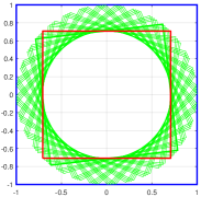
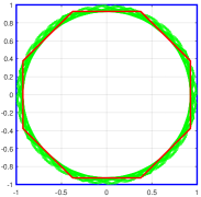
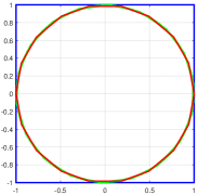
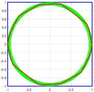
Figure 1. Computed invariant set $\mathcal{I}$ (red thick line) for the rotation example with varying numbers of generators in $\mathcal{I}$. Also shown are the constraint set $\mathcal{X}$ (blue thick line) and $\mathsf{R}\left({t},{\mathcal{I}}\right)$ (thin green lines) for $t=1,\ldots T$. Top left: Two generators (the coordinate axes). Top right: Four generators (coordinate axes plus diagonals). Bottom left: Nine generators (equally spaced around top half circle). Bottom right: Sixteen random generators (only seven have scaling $\gamma_{i}>0.01$).

To demonstrate our algorithm and the effects of the choice of $\mathrm{G}\left({\mathcal{I}}\right)$, we consider a system with rotational dynamics. Starting from the continuous time system

$$\dot{x}=\begin{bmatrix}0&-1\\ +1&0\end{bmatrix}x$$

we use the matrix exponential with time step $0.2$ to construct the discrete time system

(26) $$x(t+1)=\begin{bmatrix}+0.9801&-0.1987\\ +0.1987&+0.9801\end{bmatrix}x(t).$$

We use the optimization (24) with $\underline{x}={-\mathbf{1}_{2}}$, $\overline{x}=+\mathbf{1}_{2}$ and $T=32$ to compute an invariant set after slightly more than one full rotation. The true invariance kernel in this case is the largest circle contained in $\mathcal{X}$. Figure 1 shows the computed invariant sets with different numbers of generators in $\mathcal{I}$. Run times for the optimization were below 3 seconds for all of these examples.

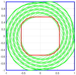
Figure 2. Computed invariant set for the rotation example with disturbance input using eight equally spaced generators for $\mathcal{I}$.

Figure 2 illustrates the results of the calculation if we introduce a disturbance with

$$\mathrm{C}=\begin{bmatrix}1&0\\ 0&1\end{bmatrix}\qquad\mathcal{V}=\left\langle\begin{bmatrix}0\\ 0\end{bmatrix}\left|\begin{bmatrix}0.05&0\\ 0&0.05\end{bmatrix}\right.\right\rangle$$

into the rotational dynamics (26).

5. Computing Viable Sets

Accommodating the disturbance input for invariant sets was notationally complicated but conceptually straightforward: The constraints on the reach sets of the initial set had to take into account the effect of an input which could take on any value in $\mathcal{V}$ at any state at any time. Achieving viability typically requires that the control input be chosen based on the current state; consequently, we need to tackle the control inputs in a different manner. To simplify the notation we work through the algorithm without disturbance inputs in this section, and consequently compute viable sets. We also omit the drift term for now.

5.1. Augmenting Generators with Control

Define the function

(27) $$\mathcal{J} (\mathcal{I},\beta,\Phi)$$

$$=\left\langle\begin{bmatrix}\alpha\\ \beta\end{bmatrix}\;\left|\;\begin{bmatrix}\gamma_{1}{g}_{1}\left({\mathcal{I}}\right)\\ \phi_{1}\end{bmatrix},\begin{bmatrix}\gamma_{2}{g}_{2}\left({\mathcal{I}}\right)\\ \phi_{2}\end{bmatrix},\ldots,\begin{bmatrix}\gamma_{p\left({\mathcal{I}}\right)}{g}_{p\left({\mathcal{I}}\right)}\left({\mathcal{I}}\right)\\ \phi_{p\left({\mathcal{I}}\right)}\end{bmatrix},\right.\right\rangle,$$

$$=\left\langle\begin{bmatrix}\alpha\\ \beta\end{bmatrix}\;\left|\;\begin{bmatrix}\mathrm{G}\left({\mathcal{I}}\right)\Gamma\\ \Phi\end{bmatrix}\right.\right\rangle,$$

where $\beta\in\mathbb{R}^{d_{u}}$, $\phi_{i}\in\mathbb{R}^{d_{u}}$ and

$$\Phi=\begin{bmatrix}\phi_{1}&\phi_{2}&\cdots&\phi_{p\left({\mathcal{I}}\right)}\end{bmatrix}\in\mathbb{R}^{d_{u}\times p\left({\mathcal{I}}\right)}.$$

Before proceeding, we note:

• The value of $\mathcal{J}(\mathcal{I},\beta,\Phi)$ is a zonotope in $\mathbb{R}^{d_{x}+d_{u}}$.

• The set $\langle\beta\mid\Phi\rangle$ is a zonotope in $\mathbb{R}^{d_{u}}$, but $\mathcal{J}(\mathcal{I},\beta,\Phi)\neq\mathcal{I}\times\langle\beta\mid\Phi\rangle$.

• Unlike the diagonal matrices $\Gamma$ (and $\Psi$ encountered below), the matrix $\Phi$ is dense: All entries may be nonzero.

• In the remainder of this work we will often refer to a collection of vectors and matrices $\{\beta(s),\Phi(s)\}_{s=0}^{t}$. The fact that the collection is parameterized by time does not imply any direct temporal dependence between its elements.

Proposition 5.1.

Given $\{\beta(s),\Phi(s)\}_{s=0}^{t-1}$ and assuming a system with no disturbance input or drift, the reach set for an initial state space zonotope $\mathcal{I}$ can be represented by a center, generator count and generator matrix given by

(28) $${c}\left({\mathsf{R}\left({t},{\mathcal{I}}\right)}\right) =\mathrm{A}^{t}\alpha+\sum_{s=0}^{t-1}\mathrm{A}^{t-1-s}\mathrm{B}\beta(s)$$

$$p\left({\mathsf{R}\left({t},{\mathcal{I}}\right)}\right) =p\left({\mathcal{I}}\right)$$

$$\mathrm{G}\left({\mathsf{R}\left({t},{\mathcal{I}}\right)}\right) =\mathrm{A}^{t}\mathrm{G}\left({\mathcal{I}}\right)\Gamma+\sum_{s=0}^{t-1}\mathrm{A}^{t-1-s}\mathrm{B}\Phi(s)$$

Proof.

For a system with $\mathcal{V}=\emptyset$ and $w=0$, the dynamics (1) can be written as the linear transform

$$x(s+1)=\begin{bmatrix}\mathrm{A}&\mathrm{B}\end{bmatrix}\begin{bmatrix}x(s)\\ u(s)\end{bmatrix}.$$

And therefore

$$\begin{bmatrix}x(0)\\ u(0)\end{bmatrix}\in\mathcal{J} (\mathcal{I},\beta(0),\Phi(0))$$

$$\;\Leftrightarrow\;x(1)\in\begin{bmatrix}\mathrm{A}&\mathrm{B}\end{bmatrix}\mathcal{J}(\mathcal{I},\beta(0),\Phi(0)),$$

$$\;\Leftrightarrow\;\mathsf{R}\left({1},{\mathcal{I}}\right)=\begin{bmatrix}\mathrm{A}&\mathrm{B}\end{bmatrix}\mathcal{J}(\mathcal{I},\beta(0),\Phi(0)).$$

Since a linear transformation of a zonotope is a zonotope, we can apply the linear transformation to (27) to determine

$$\begin{aligned} {c}\left({\mathsf{R}\left({1},{\mathcal{I}}\right)}\right)&=\mathrm{A}\alpha+\mathrm{B}\beta(0),\\ p\left({\mathsf{R}\left({1},{\mathcal{I}}\right)}\right)&=p\left({\mathcal{I}}\right),\\ \mathrm{G}\left({\mathsf{R}\left({1},{\mathcal{I}}\right)}\right)&=\mathrm{A}\mathrm{G}\left({\mathcal{I}}\right)\Gamma+\mathrm{B}\Phi(0),\end{aligned}.$$

The result (28) can then be derived by induction on $s=1,\ldots,T-1$. ∎

With this evolution formula for the initial zonotope $\mathcal{I}$, we can deduce the necessary constraints for viability.

Proposition 5.2.

Given $\{\beta(t),\Phi(t)\}_{t=0}^{T-1}$ and assuming a system with no disturbance input or drift, $\mathcal{I}\subseteq\mathsf{Viab}\left({[0,T]},{\mathcal{X}}\right)$ if

(29) $$\left(\begin{gathered}\mathrm{A}^{t}\alpha+\sum_{s=0}^{t-1}\mathrm{A}^{t-1-s}\mathrm{B}\beta(s)\\ -\left|\mathrm{A}^{t}\mathrm{G}\left({\mathcal{I}}\right)\Gamma+\sum_{s=0}^{t-1}\mathrm{A}^{t-1-s}\mathrm{B}\Phi(s)\right|\mathbf{1}_{p\left({\mathcal{I}}\right)}\end{gathered}\right) \geq\underline{x},$$

$$\left(\begin{gathered}\mathrm{A}^{t}\alpha+\sum_{s=0}^{t-1}\mathrm{A}^{t-1-s}\mathrm{B}\beta(s)\\ +\left|\mathrm{A}^{t}\mathrm{G}\left({\mathcal{I}}\right)\Gamma+\sum_{s=0}^{t-1}\mathrm{A}^{t-1-s}\mathrm{B}\Phi(s)\right|\mathbf{1}_{p\left({\mathcal{I}}\right)}\end{gathered}\right) \leq\overline{x}$$

and

(30) $$\beta(t)-\left|\Phi(t)\right|\mathbf{1}_{p\left({\mathcal{I}}\right)} \geq\underline{u},$$

$$\beta(t)+\left|\Phi(t)\right|\mathbf{1}_{p\left({\mathcal{I}}\right)} \leq\overline{u}$$

for $t=0,\ldots,T$.

Proof.

Observe that $x(0)\in\mathcal{I}$ implies $x(t)\in\mathsf{R}\left({t},{\mathcal{I}}\right)$ by (8). Define the (not necessarily unique) input

(31) $$u(t)=\beta(t)+\Phi(t)\lambda(x(t),\mathsf{R}\left({t},{\mathcal{I}}\right)).$$

By (11), $u(t)\in\langle\beta(t)\mid\Phi(t)\rangle$. By (2) and Lemma 3.1, the constraint (30) implies $\langle\beta(t)\mid\Phi(t)\rangle\subseteq\mathcal{U}$. Therefore, $u(t)\in\mathcal{U}$ for all $t=0,\ldots,T$. By (4), (28) and Lemma 3.1, the constraint (29) implies $\mathsf{R}\left({t},{\mathcal{I}}\right)\subseteq\mathcal{X}$ and consequently $x(t)\in\mathcal{X}$. We have therefore proved for any $x(0)\in\mathcal{I}$ that there exists feasible input signal $u(\cdot)$ such that the trajectory $x(\cdot)$ starting from $x(0)$ generated by $u(\cdot)$ satisfies $x(t)\in\mathcal{X}$ for $t=0,\ldots,T$. By (7), $\mathcal{I}\subseteq\mathsf{Viab}\left({[0,T]},{\mathcal{X}}\right)$. ∎

By Proposition 5.2, finding a viable set $\mathcal{I}$ reduces to finding $\alpha$, $\gamma$ and $\{\beta(t),\Phi(t)\}_{t=0}^{T-1}$ to satisfy (29) and (30). We can simply substitute (29) and (30) for (22) in the optimization (24) and add $\{\beta(t),\Phi(t)\}_{t=0}^{T-1}$ to the decision variables. A feasible solution to the resulting optimization problem will define a set of viable states through $\alpha$ and $\gamma$, and a (time dependent) set of viable controls through $\{\beta(t),\Phi(t)\}_{t=0}^{T-1}$; however, the set of viable controls may be very small: By (31) the range of $u(t)$ is directly proportional to $|\Phi(t)|$, but reducing $|\Phi(t)|$ always makes it easier to satisfy (30) and the objective from (24) provides no direct incentive to increase $|\Phi(t)|$ (although a nonzero value may be necessary to satisfy (29)).

In order to achieve a larger set of viable controls we would like to maximize $|\Phi(t)|$, but maximizing an absolute value is a non-convex objective and we are not willing to destroy the convexity of our optimization to directly incorporate such a term. We also cannot constrain $\Phi(t)\geq 0$ elementwise, since the sign of elements of $\phi_{i}(t)$ relative to the sign of elements of the corresponding ${g}_{i}\left({\mathcal{I}}\right)$ may be critical to achieving viability (more discussion in section 5.3). Another approach is needed to seek broader control authority.

5.2. Control as Scaled Disturbance

Intuitively, we would like to characterize the range of control input which could be applied while maintaining the viability of $\mathcal{I}$. That control input authority might cause the reach set to be larger than it would be otherwise, but such growth may be accommodated in regions where the state constraints are not tight. Furthermore, we already have a method of mathematically characterizing the effect of such a priori indeterminant input: Treat it as a disturbance.

With that in mind, we introduce a parameterized zonotope $\mathcal{F}$ to capture this control input authority which is independent of the authority in the equations above. Define

(32) $$\mathcal{F} =\langle\mathbf{0}_{d_{u}}\mid\psi_{1}{g}_{1}\left({\mathcal{F}}\right),\psi_{2}{g}_{2}\left({\mathcal{F}}\right),\ldots,\psi_{p\left({\mathcal{F}}\right)}{g}_{p\left({\mathcal{F}}\right)}\left({\mathcal{F}}\right)\rangle,$$

$$=\langle\mathbf{0}_{d_{u}}\mid\mathrm{G}\left({\mathcal{F}}\right)\Psi\rangle,$$

where $\Psi\in\mathbb{R}^{p\left({\mathcal{F}}\right)\times p\left({\mathcal{F}}\right)}$ is the diagonal matrix with vector $\psi$ along its diagonal. Like $\mathcal{I}$, we will fix the generators $\mathrm{G}\left({\mathcal{F}}\right)\in\mathbb{R}^{d_{u}\times p\left({\mathcal{F}}\right)}$ but leave the generator scaling vector $\psi\in\mathbb{R}^{p\left({\mathcal{F}}\right)}$ with $\psi\geq 0$ as a free parameter. We then allow for time-dependent $\mathcal{F}(t)$ and compute the result of input $u(t)\in\mathcal{F}(t)$ on the reach set according to Proposition 3.2.

Proposition 5.3.

Given $\{\beta(s),\Phi(s),\psi(s)\}_{s=0}^{t-1}$ and assuming a system with no disturbance input or drift, the reach set for an initial state space zonotope $\mathcal{I}$ can be represented by a center, generator count and generator matrix given by

(33) $${c}\left({\mathsf{R}\left({t},{\mathcal{I}}\right)}\right) =\mathrm{A}^{t}\alpha+\sum_{s=0}^{t-1}\mathrm{A}^{t-1-s}\mathrm{B}\beta(s)$$

$$p\left({\mathsf{R}\left({t},{\mathcal{I}}\right)}\right) =p\left({\mathcal{I}}\right)+\sum_{s=0}^{t-1}p\left({\mathcal{F}(s)}\right)$$

$$\mathrm{G}\left({\mathsf{R}\left({t},{\mathcal{I}}\right)}\right) =\begin{bmatrix}\mathrm{F}_{\mathcal{I}}&\mathrm{F}_{0}&\mathrm{F}_{1}&\cdots&\mathrm{F}_{t-1}\end{bmatrix}$$

where

(34) $$\mathrm{F}_{\mathcal{I}} =\mathrm{A}^{t}\mathrm{G}\left({\mathcal{I}}\right)\Gamma+\sum_{s=0}^{t-1}\mathrm{A}^{t-1-s}\mathrm{B}\Phi(s)$$

$$\mathrm{F}_{s} =\mathrm{A}^{t-1-s}\mathrm{B}\mathrm{G}\left({\mathcal{F}(s)}\right)\Psi(s)\quad\text{for }s=0,\ldots,t-1$$

Proof.

Combine (16) and (28) by superposition. ∎

We note in passing that the equation for ${c}\left({\mathsf{R}\left({t},{\mathcal{I}}\right)}\right)$ in (33) demonstrates why it is sufficient to fix the center of $\mathcal{F}(t)$ at the origin in (32): The parameter $\beta(t)$ already provides a mechanism to shift the center of the input set at time $t$.

Proposition 5.4.

Given $\{\beta(t),\Phi(t),\psi(t)\}_{t=0}^{T-1}$ and assuming a system with no disturbance input or drift, $\mathcal{I}\subseteq\mathsf{Viab}\left({[0,T]},{\mathcal{X}}\right)$ if

(35) $$\left(\begin{gathered}\mathrm{A}^{t}\alpha+\sum_{s=0}^{t-1}\mathrm{A}^{t-1-s}\mathrm{B}\beta(s)\\ -\left|\mathrm{A}^{t}\mathrm{G}\left({\mathcal{I}}\right)\Gamma+\sum_{s=0}^{t-1}\mathrm{A}^{t-1-s}\mathrm{B}\Phi(s)\right|\mathbf{1}_{p\left({\mathcal{I}}\right)}\\ -\sum_{s=0}^{t-1}\left(\left|\mathrm{A}^{t-1-s}\mathrm{B}\mathrm{G}\left({\mathcal{F}(s)}\right)\right|\psi(s)\right)\end{gathered}\right) \geq\underline{x},$$

$$\left(\begin{gathered}\mathrm{A}^{t}\alpha+\sum_{s=0}^{t-1}\mathrm{A}^{t-1-s}\mathrm{B}\beta(s)\\ +\left|\mathrm{A}^{t}\mathrm{G}\left({\mathcal{I}}\right)\Gamma+\sum_{s=0}^{t-1}\mathrm{A}^{t-1-s}\mathrm{B}\Phi(s)\right|\mathbf{1}_{p\left({\mathcal{I}}\right)}\\ +\sum_{s=0}^{t-1}\left(\left|\mathrm{A}^{t-1-s}\mathrm{B}\mathrm{G}\left({\mathcal{F}(s)}\right)\right|\psi(s)\right)\end{gathered}\right) \leq\overline{x}$$

and

(36) $$\beta(t)-\left|\Phi(t)\right|\mathbf{1}_{p\left({\mathcal{I}}\right)}-\left|\mathrm{G}\left({\mathcal{F}(t)}\right)\right|\psi(t) \geq\underline{u},$$

$$\beta(t)+\left|\Phi(t)\right|\mathbf{1}_{p\left({\mathcal{I}}\right)}+\left|\mathrm{G}\left({\mathcal{F}(t)}\right)\right|\psi(t) \leq\overline{u}$$

for $t=0,\ldots,T$.

We have shifted $\Psi(t)$ outside the absolute value in (35) and (36) because $\psi(t)\geq 0$, and then taken advantage of the fact that $\Psi(t)\mathbf{1}_{p\left({\mathcal{F}(t)}\right)}=\psi(t)$.

Proof.

Let

$$\tilde{\mathcal{U}}(t) =\langle\beta(t)\mid\begin{bmatrix}\Phi(t)&\mathrm{G}\left({\mathcal{F}(t)}\right)\Psi(t)\end{bmatrix}\rangle,$$

$$\tilde{\Phi}(t) =\begin{bmatrix}\Phi(t)&\mathbf{0}_{d_{u}\times\sum_{s=0}^{t-1}p\left({\mathcal{\mathcal{F}}(s)}\right)}\end{bmatrix},$$

and then choose any $\rho(t)\in\mathbb{R}^{p\left({\mathcal{F}(t)}\right)}$ such that

(37) $${-\mathbf{1}_{p\left({\mathcal{F}(t)}\right)}}\leq\rho(t)\leq+\mathbf{1}_{p\left({\mathcal{F}(t)}\right)}.$$

Define the input

(38) $$u(t)=\beta(t)+\tilde{\Phi}(t)\lambda(x(t),\mathsf{R}\left({t},{\mathcal{I}}\right))+\mathrm{G}\left({\mathcal{F}(t)}\right)\Psi(t)\rho(t).$$

We augment $\tilde{\Phi}(t)$ with zero columns / generators to account for the extra generators (33) in $\mathsf{R}\left({t},{\mathcal{I}}\right)$ arising from $\mathcal{F}(s)$ for $s<t$. Note that these extra generators have no direct effect on the choice of input for step $t$ in (38) because they are zero vectors, although we do need to account for their continuing effect on the choice of $\lambda(x(t),\mathsf{R}\left({t},{\mathcal{I}}\right))$ through these extra columns in $\tilde{\Phi}(t)$.

By (11), the fact that the extra generators in $\tilde{\Phi}(t)$ compared to $\Phi(t)$ are all zero vectors, and (37), $u(t)\in\tilde{\mathcal{U}}(t)$. By (2) and Lemma 3.1, the constraint (36) implies $\tilde{\mathcal{U}}(t)\subseteq\mathcal{U}$. Therefore, $u(t)\in\mathcal{U}$ for all $t=0,\ldots,T$. By (4), (33) and Lemma 3.1, the constraint (35) implies $\mathsf{R}\left({t},{\mathcal{I}}\right)\subseteq\mathcal{X}$ and consequently $x(t)\in\mathcal{X}$. The remainder is the same as the proof of Proposition 5.2. ∎

Remark 5.5.

The constraints (35) and (36) are linear in $\alpha$ and $\{\beta(t),\psi(t)\}_{t=0}^{T-1}$, and are convex in $\gamma$ and $\{\Phi(t)\}_{t=0}^{T-1}$.

Our viability optimization problem is then written as

(39) $$\max_{\alpha,\gamma,\{\beta(t),\Phi(t),\psi(t)\}_{t=0}^{T-1}} \mathbf{1}_{p\left({\mathcal{I}}\right)}^{T}\gamma+\eta\sum_{t=0}^{T-1}\mathbf{1}_{p\left({\mathcal{F}(t)}\right)}^{T}\psi(t)$$

such that $$\gamma\geq 0$$

$$\psi(t)\geq 0$$

and $$\text{(\ref{e:viable-state-control-disturb-box-containment}),~{}(\ref{e:viable-input-control-disturb-box-containment}) hold }\forall t\in 0,\ldots,T$$

where $\eta>0$ is a weighting parameter used to trade off the relative importance of large $\gamma$ (to encourage a larger set of viable states) against large $\psi(t)$ (to encourage a larger set of viable controls).

Remark 5.6.

The optimization (39) is a convex program with $d_{x}+p\left({\mathcal{I}}\right)+Td_{u}(p\left({\mathcal{I}}\right)+1)+\sum_{t}p\left({\mathcal{F}(t)}\right)$ decision variables, $p\left({\mathcal{I}}\right)+\sum_{t}p\left({\mathcal{F}(t)}\right)$ non-negativity constraints, and $2(d_{x}+d_{u})(T+1)$ general convex constraints from (35) and (36).

5.3. Example: Double Integrator

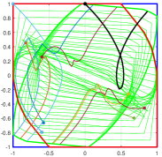
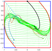
Figure 3. Computed viable set $\mathcal{I}$ (red thick line) for the double integrator example with (left) and without (right) $\mathcal{F}$. Eight generators equally spaced in the north-west quadrant are used (only five have scaling $\gamma_{i}>0.01$). Also shown are the constraint set $\mathcal{X}$ (blue thick line), $\mathsf{R}\left({\mathcal{I}},{t}\right)$ (thin green lines) for $t=1,\ldots T$, and a collection of sample trajectories (star shows the initial conditions for each).

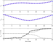
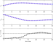
Figure 4. Sample viable trajectory (shown as the thick black trajectory in figure 3) with (left) and without (right) $\mathcal{F}$. Control at each time is chosen as close to $+1$ as possible subject to (38) on the left and (31) on the right. The dotted curve in the control subplot shows the scaling $\psi_{1}(t)$ (which is always zero on the right). Any difference between the actual control $u_{1}(t)$ and scaling $\psi_{1}(t)$ arises from $\Phi(t)$.

To demonstrate the viability algorithm we consider the traditional double integrator. Starting from the continuous time system

$$\dot{x}=\begin{bmatrix}0&+1\\ 0&0\end{bmatrix}x+\begin{bmatrix}0\\ 1\end{bmatrix}u$$

we use the matrix exponential with time step $0.1$ and Matlab’s integral() adaptive quadrature routine to construct the discrete time system

$$x(t+1)=\begin{bmatrix}+1.0000&+0.1000\\ 0&+1.0000\end{bmatrix}x(t)+\begin{bmatrix}+0.0050\\ +0.1000\end{bmatrix}u(t).$$

We use the optimization (39) with $d_{x}=2$, $d_{u}=1$, $\underline{x}={-\mathbf{1}_{d_{x}}}$, $\overline{x}=+\mathbf{1}_{d_{x}}$, $\underline{u}=-1$, $\overline{u}=+1$, and $T=30$ to compute a viable set, and in the process demonstrate the importance of including characterizations of control authority from both sections 5.1 and 5.2. Figure 3 shows the computed viable set with and without the additional control authority enabled by the technique from section 5.2 (with $\mathcal{F}(t)$ equal to the $2\times 2$ identity matrix for all $t$). Run time for the optimization was below 5 seconds for both cases.

No viable set is found if we omit $\Phi(t)$ from section 5.1, so that case is not shown. Some intuition for the failure of this latter case to find any viable set can be found by examining $\phi_{1}(t)$ for the other cases. This input component corresponds to the state generator ${g}_{1}\left({\mathcal{I}}\right)=\begin{bmatrix}0&1\end{bmatrix}^{T}$, which is the generator whose scaling to a large extent determines the height of the viable set. For the first half of the time horizon, $\phi_{1}(t)<0$; in other words, states that have a large positive velocity $x_{2}(t)$ will be forced (through $\lambda(x(t),\mathsf{R}\left({t},{\mathcal{I}}\right))$ in (31) or (38)) to choose a correspondingly large negative control input $u(t)$. Without the coupling of state and input signal through $\Phi(t)$, viability is infeasible. Figure 4 shows a single trajectory’s states and control input componentwise over time and displays just this behavior: Although the desired input is $+1$, the early input signal $u(t)$ is forced to be negative because $x_{2}(t)$ is quite positive.

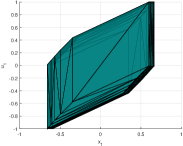
Figure 5. Projection of the set of viable inputs at $t=20$ with (left) and without (right) $\mathcal{F}$.

At later times $\phi_{1}(t)$ does become slightly positive, but it is at these times toward the end of the viability horizon that the benefits of section 5.2 are visible. Although the sets of viable states in figure 3 are the same with or without $\mathcal{F}$, the set of viable controls is notably larger if we include a non-empty $\mathcal{F}$; for example, figure 5 shows that the set of viable controls at $t=20$ is much larger on the left, while on the left of figure 4 $u_{1}(t)$ is much more able to approach the target value of $+1$ in the latter half of the horizon because of the growth of $\psi_{1}(t)$.

6. Computing Discriminating Sets

In this section we incorporate the control, disturbance and drift terms by combining the derivations in Sections 4.2 and 5.2 to handle the full generality of the dynamics (1). The longer equations referenced in this section are collected in figure 6.

(40) $$\left.\begin{aligned} {c}\left({\mathsf{R}\left({t},{\mathcal{I}}\right)}\right)&=\mathrm{A}^{t}\alpha+\sum_{s=0}^{t-1}\mathrm{A}^{t-1-s}\left(\mathrm{B}\beta(s)+\mathrm{C}{c}\left({\mathcal{V}}\right)+w\right),\\ p\left({\mathsf{R}\left({t},{\mathcal{I}}\right)}\right)&=p\left({\mathcal{I}}\right)+\sum_{s=0}^{t-1}p\left({\mathcal{F}(s)}\right)+tp\left({\mathcal{V}}\right)\\ \mathrm{G}\left({\mathsf{R}\left({t},{\mathcal{I}}\right)}\right)&=\begin{bmatrix}\mathrm{F}_{\mathcal{I}}&\mathrm{F}_{0}&\mathrm{F}_{1}&\cdots&\mathrm{F}_{t-1}&\mathrm{A}^{t-1}\mathrm{C}\mathrm{G}\left({\mathcal{V}}\right)&\mathrm{A}^{t-2}\mathrm{C}\mathrm{G}\left({\mathcal{V}}\right)&\cdots&\mathrm{C}\mathrm{G}\left({\mathcal{V}}\right)\end{bmatrix}\end{aligned}\right\}\begin{gathered}\text{where }\mathrm{F}_{\mathcal{I}}\text{ and }\{\mathrm{F}_{s}\}_{s=0}^{t-1}\\ \text{are given in~{}(\ref{e:control-disturb-generator-defn})}.\end{gathered}$$

(41) $$\left.\begin{aligned} \left(\begin{gathered}\mathrm{A}^{t}\alpha+\sum_{s=0}^{t-1}\mathrm{A}^{t-1-s}\left(\mathrm{B}\beta(s)+\mathrm{C}{c}\left({\mathcal{V}}\right)+w\right)-\left|\mathrm{A}^{t}\mathrm{G}\left({\mathcal{I}}\right)\Gamma+\sum_{s=0}^{t-1}\mathrm{A}^{t-1-s}\mathrm{B}\Phi(s)\right|\mathbf{1}_{p\left({\mathcal{I}}\right)}\\ -\sum_{s=0}^{t-1}\left(\left|\mathrm{A}^{t-1-s}\mathrm{B}\mathrm{G}\left({\mathcal{F}(s)}\right)\right|\psi(s)\right)-\sum_{s=0}^{t-1}\left(\left|\mathrm{A}^{t-1-s}\mathrm{C}\mathrm{G}\left({\mathcal{V}}\right)\right|\mathbf{1}_{p\left({\mathcal{V}}\right)}\right)\end{gathered}\right)&\geq\underline{x},\\ \left(\begin{gathered}\mathrm{A}^{t}\alpha+\sum_{s=0}^{t-1}\mathrm{A}^{t-1-s}\left(\mathrm{B}\beta(s)+\mathrm{C}{c}\left({\mathcal{V}}\right)+w\right)+\left|\mathrm{A}^{t}\mathrm{G}\left({\mathcal{I}}\right)\Gamma+\sum_{s=0}^{t-1}\mathrm{A}^{t-1-s}\mathrm{B}\Phi(s)\right|\mathbf{1}_{p\left({\mathcal{I}}\right)}\\ +\sum_{s=0}^{t-1}\left(\left|\mathrm{A}^{t-1-s}\mathrm{B}\mathrm{G}\left({\mathcal{F}(s)}\right)\right|\psi(s)\right)+\sum_{s=0}^{t-1}\left(\left|\mathrm{A}^{t-1-s}\mathrm{C}\mathrm{G}\left({\mathcal{V}}\right)\right|\mathbf{1}_{p\left({\mathcal{V}}\right)}\right)\end{gathered}\right)&\leq\overline{x}\end{aligned}\right\}\text{for }t=0,\ldots,T.$$

Figure 6. Some long equations for Propositions 6.1 and 6.2.

Proposition 6.1.

Given $\{\beta(s),\Phi(s),\psi(s)\}_{s=0}^{t-1}$, the reach set for an initial state space zonotope $\mathcal{I}$ can be represented by a center, generator count and generator matrix given by (40).

Proof.

Combine (16) and (33) by superposition. ∎

Proposition 6.2.

Given $\{\beta(t),\Phi(t),\psi(t)\}_{t=0}^{T-1}$, if (36) and (41) hold then $\mathcal{I}\subseteq\mathsf{Disc}\left({[0,T]},{\mathcal{X}}\right)$.

Proof.

Redefine

$$\tilde{\Phi}(t)=\begin{bmatrix}\Phi(t)&\mathbf{0}_{d_{u}\times\sum_{s=0}^{t-1}p\left({\mathcal{\mathcal{F}}(s)}\right)}&\mathbf{0}_{d_{u}\times tp\left({\mathcal{V}}\right)}\end{bmatrix},$$

to account for the extra columns / generators in $\mathrm{G}\left({\mathsf{R}\left({t},{\mathcal{I}}\right)}\right)$ arising from the disturbance inputs, and then combine the proofs of Propositions 4.5 and 5.4 by superposition. ∎

6.1. Example: Nonlinear Quadrotor

(42) $$\begin{bmatrix}\dot{x}_{1}\\ \dot{x}_{2}\\ \dot{x}_{3}\\ \dot{x}_{4}\\ \dot{x}_{5}\\ \dot{x}_{6}\end{bmatrix}=\overbrace{\begin{bmatrix}0&0&1&0&0&0\\ 0&0&0&1&0&0\\ 0&0&0&0&+K\bar{u}_{1}\cos\bar{x}_{5}&0\\ 0&0&0&0&-K\bar{u}_{1}\sin\bar{x}_{5}&0\\ 0&0&0&0&0&1\\ 0&0&0&0&-d_{0}&-d_{1}\end{bmatrix}}^{\mathrm{A}}\overbrace{\begin{bmatrix}x_{1}\\ x_{2}\\ x_{3}\\ x_{4}\\ x_{5}\\ x_{6}\end{bmatrix}}^{x}+\overbrace{\begin{bmatrix}0&0\\ 0&0\\ K\sin\bar{x}_{5}&0\\ K\cos\bar{x}_{5}&0\\ 0&0\\ 0&n_{0}\end{bmatrix}}^{\mathrm{B}}\overbrace{\begin{bmatrix}u_{1}\\ u_{2}\end{bmatrix}}^{u}+\overbrace{\begin{bmatrix}0&0\\ 0&0\\ 1&0\\ 0&1\\ 0&0\\ 0&0\end{bmatrix}}^{\mathrm{C}}\overbrace{\begin{bmatrix}v_{1}\\ v_{2}\end{bmatrix}}^{v}+\overbrace{\begin{bmatrix}0\\ 0\\ -K\bar{u}_{1}\sin\bar{x}_{5}\\ +K\bar{u}_{1}\cos\bar{x}_{5}-g\\ 0\\ 0\end{bmatrix}}^{w}$$

Figure 7. Linearized quadrotor dynamics.

To demonstrate the utility of the full algorithm, we compute a discriminating set for a partially nonlinear six dimensional longitudinal model of a quadrotor taken from (Bouffard, 2012). The state space dimensions are:

• horizontal position $x_{1}$ [m] (positive rightward),

• vertical position $x_{2}$ [m] (positive upward),

• horizontal velocity $x_{3}$ [m/s],

• vertical velocity $x_{4}$ [m/s],

• roll $x_{5}$ [rad] (positive clockwise),

• roll velocity $x_{6}$ [rad/s].
  

The control input dimensions are:

• total thrust $u_{1}$,

• desired roll angle $u_{2}$.
  

The nonlinear continuous time plant dynamics model is:

(43a) $$\dot{x}_{1} =x_{3},$$

(43b) $$\dot{x}_{2} =x_{4},$$

(43c) $$\dot{x}_{3} =u_{1}K\sin x_{5},$$

(43d) $$\dot{x}_{4} =-g+u_{1}K\cos x_{5},$$

(43e) $$\dot{x}_{5} =x_{6},$$

(43f) $$\dot{x}_{6} =-d_{0}x_{5}-d_{1}x_{6}+n_{0}u_{2},$$

We adopt the constraint set used in (Mitchell et al., 2016), except that we broaden the range of $x_{5}$:

(44) $$x_{1} \in[-1.7,+1.7],$$

$$x_{2} \in[+0.3,+2.0],$$

$$x_{3} \in[-0.8,+0.8],$$

$$x_{4} \in[-1.0,+1.0],$$

$$x_{5} \in[-\tfrac{\pi}{12},+\tfrac{\pi}{12}],$$

$$x_{6} \in[-\tfrac{\pi}{2},+\tfrac{\pi}{2}].$$

We also broaden the range of allowed controls:

(45) $$u_{1} \in[-1.5,+1.5]+\bar{u}_{1},$$

$$u_{2} \in[-\tfrac{\pi}{12},+\tfrac{\pi}{12}]+\bar{x}_{5},$$

where $\bar{u}_{1}=g/K$ and $\bar{x}_{5}=0$. We then linearize (43) about $\bar{u}_{1}$ and $\bar{x}_{5}$ to arrive at the linear model (42). Note that unlike (Mitchell et al., 2016) we do not hybridize the dynamics in order to linearize about multiple operating points; the entire constraint set is handled with a single linear model. For the range of $x_{5}$ in (44) and $u_{1}$ in (45), the linearization errors are

$$\text{error in }\dot{x}_{3} \in[-0.2760,+0.2760],$$

$$\text{error in }\dot{x}_{4} \in[0.0000,+0.3668].$$

For conservativeness, we choose $\mathcal{V}$ to be this error rectangle dilated by $10\%$. Note that the disturbance affects only $x_{3}$ and $x_{4}$ because the dynamics of the remaining dimensions are exactly linear. The parameter values used in simulation are taken from (Mitchell et al., 2016): $K=0.89/1.4$, $d_{0}=70$, $d_{1}=17$ and $n_{0}=55$.

We use Matlab’s expm() and integral() routines to construct the discrete time version of (42) with time step $0.05$, and then compute for a horizon $T=40$. To choose generators, we note that for $\bar{x}_{5}=0$ the pairs of dimensions $\{(x_{1},x_{3}),(x_{2},x_{4}),(x_{3},x_{5}),(x_{5},x_{6})\}$ look like double integrators. For these pairs we create five generators in the north-west quadrant, while for the remaining pairs of states we create only two generators along the diagonal and anti-diagonal. To these we add the six coordinate axes for a total of $p\left({\mathcal{I}}\right)=48$ generators. We also tried running the optimization with an additional 52 randomly oriented generators to see whether coupling between more than two dimensions would improve the discriminating set; however, none of the randomly oriented generators achieved a scaling $\gamma_{i}\geq 0.01$ and so we discarded them in subsequent runs.

Figure 8. Projections of the computed discriminating set $\mathcal{I}$ (red thick line) for the quadrotor model.

We run the optimization problem (39) with constraint (41) substituted for (35). Run time for the optimization is just over 5 minutes. Only 11 of the 48 generators achieved a scaling factor $\gamma_{i}\geq 0.01$. Figure 8 shows projections of the resulting discriminating set. Note that this set is discriminating for both the linear and nonlinear models, since we conservatively capture all linearization error in the disturbance input bounds.

Although we have insufficient space to make a detailed comparison with the ellipsoid-based results from (Mitchell et al., 2016), we can observe that in roughly the same computational time (albeit on a slightly faster laptop) our zonotope-based algorithm is able to find a much larger discriminating set over twice the time horizon with double the time resolution. Furthermore, the zonotope representation is much less conservative with its treatment of the disturbance input, and hence we do not need to hybridize or to restrict the range of $x_{5}$ and $u_{1}$ so severely. We hypothesize that most of the improvement in accuracy arises from the fact that zonotopes can exactly represent the rectangular form of typical state and input constraints, while ellipsoids are forced to adopt dramatic under- or over-approximations.

7. Discussion

The formulations developed above leave a number of parameters to be chosen by the user and make some assumptions which could be relaxed. We briefly discuss these issues in this section.

The key parameter open to the user is the choice of generators $\mathrm{G}\left({\mathcal{I}}\right)$ and $\mathrm{G}\left({\mathcal{F}(t)}\right)$. Unless there is some reason to believe that direct coupling of the inputs is beneficial, the latter will typically be chosen as an identity matrix. Choosing the former is trickier; however, the experience in section 6.1 indicates that examination of the sparsity pattern of $\mathrm{A}$ may allow one to choose these vectors more efficiently than simply trying to cover the unit hypersphere in $\mathbb{R}^{d_{x}}$.

One factor that is perhaps not so obvious when choosing generators is that this choice impacts the quality of the resulting sets not just directly through the generators but also indirectly through the heuristic objective function in (39). If $\mathrm{G}\left({\mathcal{I}}\right)$ is orthonormal then $\max\mathbf{1}_{p\left({\mathcal{I}}\right)}^{T}\gamma$ is not an unreasonable heuristic to make $\mathcal{I}$ large, but as the generators lose perpendicularity (inevitable as the number of generators grows) the quality of this heuristic decreases. It should be noted that this heuristic appears to encourage sparse $\gamma$, which could be a significant benefit for downstream uses of $\mathcal{I}$.

Finally, the restriction to interval hulls of the control input set $\mathcal{U}$ and constraint set $\mathcal{X}$ was driven by the need to include constraints in the optimization which confirmed that (projections of) zonotopes were contained within those sets. That restriction can be relaxed to any class of sets for which a reasonable number of constraints can confirm zonotope containment; for example, intersections of slabs, or even convex polygons with a modest number of faces. It may even be possible to allow full zonotopes using (Han et al., 2016, Lemma 3), albeit at the cost of swapping a small number of constraints (such as (36)) for a full linear matrix inequality.

8. Conclusions and Future Work

We have derived convex optimizations whose solutions represent invariant, viable or discriminating sets for discrete time, continuous state affine dynamical systems, and demonstrated the results on a simple rotation, a double integrator and a six dimensional nonlinear longitudinal model of a quadrotor respectively. The optimizations can be solved with modest computing power in seconds to minutes.

A key shortcoming of the current formulation is its restriction to discrete time. Unfortunately, the typical approaches to soundly mapping continuous time reachability into discrete time reachability (for example, see (Althoff and Frehse, 2016)) cannot be used in our approach, so we are exploring alternatives.

We are hopeful that some of the computational efficiency techniques demonstrated in (Bak and Duggirala, 2017; Bogomolov et al., 2018) could be applied to improve the scalability of the optimization problems derived here. Although there are pruning heuristics which could be applied to reduce the number of generators, the size of the optimization inevitably grows with finer time discretization and/or longer horizons. We have considered approaches to replace one large optimization with many smaller ones, although there are tradeoffs in such schemes.

Finally, we are exploring the use of the viable and discriminating sets for classifying and filtering exogenous control inputs at run-time.

- (1)
- Althoff (2010) Matthias Althoff. 2010. Reachability Analysis and its Application to the Safety Assessment of Autonomous Cars. Ph.D. Dissertation.
- Althoff (2015) Matthias Althoff. 2015. An introduction to CORA 2015. In In Proc. of the Workshop on Applied Verification for Continuous and Hybrid Systems. 120–151.
- Althoff and Frehse (2016) Matthias Althoff and Goran Frehse. 2016. Combining zonotopes and support functions for efficient reachability analysis of linear systems. In IEEE Conference on Decision and Control (CDC). 7439–7446.
- Althoff and Krogh (2011) Matthias Althoff and Bruce H. Krogh. 2011. Zonotope Bundles for the Efficient Computation of Reachable Sets. In IEEE Conference on Decision and Control (CDC). 6814–6821.
- Aubin et al. (2011) Jean-Pierre Aubin, Alexandre M. Bayen, and Patrick Saint-Pierre. 2011. Viability Theory: New Directions. Springer. https://doi.org/10.1007/978-3-642-16684-6
- Bak and Duggirala (2017) Stanley Bak and Parasara Duggirala. 2017. HyLAA: A Tool for Computing Simulation-Equivalent Reachability for Linear Systems. In Hybrid Systems: Computation and Control (HSCC).
- Bogomolov et al. (2018) Sergiy Bogomolov, Marcelo Forets, Goran Frehse, Frédéric Viry, Andreas Podelski, and Christian Schilling. 2018. Reach Set Approximation Through Decomposition with Low-dimensional Sets and High-dimensional Matrices. In Hybrid Systems: Computation and Control (HSCC). 41–50. https://doi.org/10.1145/3178126.3178128
- Bouffard (2012) Patrick Bouffard. 2012. On-board Model Predictive Control of a Quadrotor Helicopter: Design, Implementation, and Experiments. Technical Report UCB/EECS-2012-241. Department of Electrical Engineering and Computer Science, University of California at Berkeley. http://www.eecs.berkeley.edu/Pubs/TechRpts/2012/EECS-2012-241.html
- Girard (2005) Antoine Girard. 2005. Reachability of Uncertain Linear Systems using Zonotopes. In Hybrid Systems: Computation and Control (HSCC), Manfred Morari and Lothar Thiele (Eds.). Number 3414 in Lecture Notes in Computer Science. Springer Verlag, 291–305. https://doi.org/10.1007/978-3-540-31954-2_19
- Girard et al. (2006) Antoine Girard, Colas Le Guernic, and Oded Maler. 2006. Efficient Computation of Reachable Sets of Linear Time-Invariant Systems with Inputs. In Hybrid Systems: Computation and Control (HSCC), João Hespanha and Ashish Tiwari (Eds.). Number 3927 in Lecture Notes in Computer Science. Springer Verlag, 257–271.
- Gover and Krikorian (2010) Eugene Gover and Nishan Krikorian. 2010. Determinants and the volumes of parallelotopes and zonotopes. Linear Algebra Appl. 433, 1 (2010), 28 – 40. https://doi.org/10.1016/j.laa.2010.01.031
- Grant and Boyd (2008) Michael Grant and Stephen Boyd. 2008. Graph implementations for nonsmooth convex programs. In Recent Advances in Learning and Control, V. Blondel, S. Boyd, and H. Kimura (Eds.). Springer-Verlag Limited, 95–110. http://stanford.edu/~boyd/graph_dcp.html.
- Grant and Boyd (2017) Michael Grant and Stephen Boyd. 2017. CVX: Matlab Software for Disciplined Convex Programming, version 2.1. http://cvxr.com/cvx. (Dec. 2017).
- Han et al. (2016) Dongkun Han, Albert Rizaldi, Ahmed El-Guindy, and Matthias Althoff. 2016. On enlarging backward reachable sets via Zonotopic set membership. In IEEE Int. Symp. on Intelligent Control (ISIC). 1–8.
- Maidens et al. (2013) John N. Maidens, Shahab Kaynama, Ian M. Mitchell, Meeko M. K. Oishi, and Guy A. Dumont. 2013. Lagrangian Methods for Approximating the Viability Kernel in High-Dimensional Systems. Automatica 49, 7 (July 2013), 2017–2029. https://doi.org/10.1016/j.automatica.2013.03.020
- Mitchell and Kaynama (2015) Ian M. Mitchell and Shahab Kaynama. 2015. An Improved Algorithm for Robust Safety Analysis of Sampled Data Systems. In Hybrid Systems: Computation and Control (HSCC). 21–30. https://doi.org/10.1145/2728606.2728619
- Mitchell et al. (2016) Ian M. Mitchell, Jeffrey Yeh, Forrest J. Laine, and Claire J. Tomlin. 2016. Ensuring Safety for Sampled Data Systems: An Efficient Algorithm for Filtering Potentially Unsafe Input Signals. In IEEE Conference on Decision and Control (CDC). Las Vegas, NV, 7431–7438. https://doi.org/10.1109/CDC.2016.7799417
- Schürmann and Althoff (2017a) Bastian Schürmann and Matthias Althoff. 2017a. Convex interpolation control with formal guarantees for disturbed and constrained nonlinear systems. In Hybrid Systems: Computation and Control (HSCC). 121–130. https://doi.org/10.1145/3049797.3049800
- Schürmann and Althoff (2017b) Bastian Schürmann and Matthias Althoff. 2017b. Guaranteeing constraints of disturbed nonlinear systems using set-based optimal control in generator space. In International Federation of Automatic Control (IFAC) World Congress.
- Schürmann and Althoff (2017c) Bastian Schürmann and Matthias Althoff. 2017c. Optimal control of sets of solutions to formally guarantee constraints of disturbed linear systems. In American Control Conference (ACC). 2522–2529. https://doi.org/10.23919/ACC.2017.7963332