A two-dimensional soliton system of vortex and Q-ball

Abstract

The $(2+1)$-dimensional gauge model describing two complex scalar fields that interact through a common Abelian gauge field is considered. It is shown that the model has a soliton solution that describes a system consisting of a vortex and a Q-ball. This two-dimensional system is electrically neutral, nevertheless it possesses a nonzero electric field. Moreover, the soliton system has a quantized magnetic flux and a nonzero angular momentum. Properties of this vortex-Q-ball system are investigated by analytical and numerical methods. It is found that the system combines properties of topological and nontopological solitons.

1 Introduction

Topological solitons of $(2+1)$-dimensional field models play an important role in field theory, physics of condensed state, cosmology, and hydrodynamics. First of all, it is necessary to mention vortices of the effective theory of superconductivity [1] and vortices of the $(2+1)$-dimensional Abelian Higgs model [2]. Another important example is given by the soliton solution of the $(2+1)$-dimensional nonlinear $O(3)$ $\sigma$ model [3] that effectively describes the behavior of a ferromagnet in the critical region.

Two-dimensional soliton solutions of Abelian Maxwell gauge models are necessarily electrically neutral. This is because the $(2+1)$-dimensional Maxwell electrodynamics does not admit the existence of electrically charged spatially localized solutions with finite energy [4], in contrast to the $(3+1)$-dimensional case. However, the electrical neutrality does not forbid the existence of two-dimensional solitons possessing an electric field.

In this Letter we consider a two-dimensional soliton system consisting of an Abelian vortex and a Q-ball. The vortex and the Q-ball interact through a common Abelian gauge field. This electrically neutral soliton system possesses a radial electric field, carries a quantized magnetic flux, and has a nonzero angular momentum. The soliton system combines the properties of vortex and Q-ball. The interaction between the vortex and the Q-ball by means of a common gauge field leads to a significant change of their shapes.

2 Lagrangian and field equations of the model

The $(2+1)$-dimensional model we are interested in is described by the Lagrangian density

$$\mathcal{L} = -\frac{1}{4}F_{\mu\nu}F^{\mu\nu}+\left(D_{\mu}\phi\right)^{\ast}D^{\mu}\phi-V\left(\left|\phi\right|\right)$$ (1)

$$+\left(D_{\mu}\chi\right)^{\ast}D^{\mu}\chi-U\left(\left|\chi\right|\right),$$

where $\phi$ and $\chi$ are complex scalar fields that are minimally coupled to the Abelian gauge field $A_{\mu}$ through covariant derivatives:

$$D_{\mu}\phi=\partial_{\mu}\phi-ieA_{\mu}\phi,\quad D_{\mu}\chi=\partial_{\mu}\chi-iqA_{\mu}\chi.$$ (2)

The self-interaction potentials $V\left(\left|\phi\right|\right)$ and $U\left(\left|\chi\right|\right)$ are

$$V\left(\left|\phi\right|\right) =\frac{\lambda}{2}\left(\phi^{\ast}\phi-v^{2}\right)^{2}\!,$$

$$U\left(\left|\chi\right|\right) =m^{2}\chi^{\ast}\chi-g\left(\chi^{\ast}\chi\right)^{2}+h\left(\chi^{\ast}\chi\right)^{3}\!,$$ (3)

where $\lambda$, $g$, and $h$ are the positive self-interaction constants, $m$ is the mass of the scalar $\chi$-particle, and $v$ is the vacuum average of the complex scalar field $\phi$. We suppose that the potential $U\left(\left|\chi\right|\right)$ has the global minimum at $\chi=0$ and a local one at some $\left|\chi\right|\neq 0$; hence we have the following condition for the parameters $m$, $g$, and $h$:

$$\frac{g^{2}}{4m^{2}}<h<\frac{g^{2}}{3m^{2}}.$$ (4)

Note that if the coupling constant $q$ in Eq. (2) is set equal to zero, then model (1) has the soliton solution describing an Abelian vortex and a two-dimensional Q-ball. However, there is no electric field in this case, so the vortex and the Q-ball do not interact with each other.

The Lagrangian (1) is invariant under the local gauge transformations:

$$\phi\left(x\right) \rightarrow \phi^{\prime}\left(x\right)=\exp\left(ie\Lambda\left(x\right)\right)\phi\left(x\right),$$

$$\chi\left(x\right) \rightarrow \chi^{\prime}\left(x\right)=\exp\left(iq\Lambda\left(x\right)\right)\chi\left(x\right),$$

$$A_{\mu}\left(x\right) \rightarrow A_{\mu}^{\prime}\left(x\right)=A_{\mu}\left(x\right)+\partial_{\mu}\Lambda\left(x\right).$$ (5)

Moreover, the Lagrangian (1) is also invariant under the two independent global gauge transformations:

$$\phi\left(x\right) \rightarrow \phi^{\prime}\left(x\right)=\exp\left(i\alpha\right)\phi\left(x\right),$$

$$\chi\left(x\right) \rightarrow \chi^{\prime}\left(x\right)=\exp\left(i\beta\right)\chi\left(x\right).$$ (6)

The corresponding Noether currents are

$$j_{\phi}^{\mu} = -i\left[\phi^{\ast}D^{\mu}\phi-\left(D^{\mu}\phi\right)^{\ast}\phi\right],$$

$$j_{\chi}^{\mu} = -i\left[\chi^{\ast}D^{\mu}\chi-\left(D^{\mu}\chi\right)^{\ast}\chi\right].$$ (7)

By varying the action $S=\int\mathcal{L}d^{3}x$ in $A_{\mu}$, $\phi^{\ast}$, and $\chi^{\ast}$, we obtain the field equations of the model:

$$\partial_{\mu}F^{\mu\nu}=j^{\nu},$$ (8)

$$D_{\mu}D^{\mu}\phi+\lambda\left(\phi^{\ast}\phi-v^{2}\right)\phi=0,$$ (9)

$$D_{\mu}D^{\mu}\chi+\left(m^{2}-2g\left(\chi^{\ast}\chi\right)+3h\left(\chi^{\ast}\chi\right)^{2}\right)\chi=0,$$ (10)

where the electromagnetic current $j^{\mu}$ is expressed in terms of Noether currents:

$$j^{\mu}=ej_{\phi}^{\mu}+qj_{\chi}^{\mu}.$$ (11)

Using the well-known formula $T_{\mu\nu}\!=\!2\partial\mathcal{L}/\partial g^{\mu\nu}\!-g^{\mu\nu}\mathcal{L}$, we obtain the symmetric energy-momentum tensor of the model

$$T_{\mu\nu}= -F_{\mu\lambda}F_{\nu}^{\;\lambda}+\frac{1}{4}g_{\mu\nu}F_{\lambda\rho}F^{\lambda\rho}$$

$$+\left(D_{\mu}\phi\right)^{\ast}D_{\nu}\phi+\left(D_{\nu}\phi\right)^{\ast}D_{\mu}\phi$$

$$-g_{\mu\nu}\left(\left(D_{\mu}\phi\right)^{\ast}D^{\mu}\phi-V\left(\left|\phi\right|\right)\right)$$

$$+\left(D_{\mu}\chi\right)^{\ast}D_{\nu}\chi+\left(D_{\nu}\chi\right)^{\ast}D_{\mu}\chi$$

$$-g_{\mu\nu}\left(\left(D_{\mu}\chi\right)^{\ast}D^{\mu}\chi-U\left(\left|\chi\right|\right)\right).$$ (12)

In particular, the energy density can be written as

$$T_{00}= \frac{1}{2}E_{i}E_{i}+\frac{1}{2}B^{2}$$ (13)

$$+\left(D_{0}\phi\right)^{\ast}D_{0}\phi+\left(D_{i}\phi\right)^{\ast}D_{i}\phi+V\left(\left|\phi\right|\right)$$

$$+\left(D_{0}\chi\right)^{\ast}D_{0}\chi+\left(D_{i}\chi\right)^{\ast}D_{i}\chi+U\left(\left|\chi\right|\right),$$

where $E_{i}=F_{0i}$ are the components of electric field strength and $B=-F_{12}$ is the magnetic field strength.

Let us fix the gauge as follows: $\partial_{0}\phi=0$. We want to find a soliton solution of model (1) that minimizes the energy functional $E=\int T_{00}d^{2}x$ at the fixed value of the Noether charge $Q_{\chi}=\int j_{\chi}^{0}d^{2}x$. From the method of Lagrange multipliers it follows that the soliton is an unconditional extremum of the functional

$$F=\int\mathcal{H}d^{2}x-\omega\int j_{\chi}^{0}d^{2}x=E-\omega Q_{\chi},$$ (14)

where $\mathcal{H}$ is the Hamiltonian density and $\omega$ is the Lagrange multiplier. Let us write the Noether charge $Q_{\chi}$ in terms of the canonically conjugated variables:

$$Q_{\chi}=i\int\left(\chi\pi_{\chi}-\chi^{\ast}\pi_{\chi^{\ast}}\right)d^{2}x,$$ (15)

where $\pi_{\chi}=\partial\mathcal{L}/\partial\left(\partial_{0}\chi\right)=\left(D_{0}\chi\right)^{\ast}$ and $\pi_{\chi^{\ast}}=\partial\mathcal{L}/\partial\left(\partial_{0}\chi^{\ast}\right)=D_{0}\chi$ are the generalized momenta canonically conjugated to $\chi$ and $\chi^{\ast}$, respectively.

The extremum condition for the functional $F$ is written as

$$\delta F=\delta H-\omega\delta Q_{\chi}=0,$$ (16)

where a variation of the Noether charge $Q_{\chi}$ is written in terms of the canonically conjugate variables:

$$\delta Q_{\chi}=i\int\left(\chi\delta\pi_{\chi}+\pi_{\chi}\delta\chi-\text{c.c.}\right)d^{2}x.$$ (17)

Using the Hamilton field equations and Eqs. (16) and (17), we obtain:

$$\partial_{0}\chi=\frac{\delta H}{\delta\pi_{\chi}}=i\omega\chi,\quad\partial_{0}\chi^{\ast}=\frac{\delta H}{\delta\pi_{\chi^{\ast}}}=-i\omega\chi^{\ast},$$ (18)

while time derivatives of the other model’s fields are equal to zero. From Eq. (18) we get the time dependence of the scalar field $\chi$

$$\chi\left(x\right)=\chi\left(\mathbf{x}\right)\exp\left(i\omega t\right),$$ (19)

whereas the other fields of the model do not depend on time in the gauge $\partial_{0}\phi=0$. From Eq. (16) it follows that the important relation holds for the soliton solution:

$$\frac{dE}{dQ_{\chi}}=\omega,$$ (20)

where $\omega$ is some function of $Q_{\chi}$.

3 The ansatz and some properties of the solution

To find the soliton solution of field equations (8), (9), and (10), we use the following ansatz for the model’s fields:

$$A^{\mu}\left(x\right) =\left(\frac{A_{0}\left(r\right)}{er},\frac{1}{er}\epsilon_{ij}n_{j}A\left(r\right)\right),$$

$$\phi\left(x\right) =v\exp\left(-iN\theta\right)F\left(r\right),$$

$$\chi\left(x\right) =\sigma\left(r\right)\exp\left(i\omega t\right),$$ (21)

where $\epsilon_{ij}$ and $n_{j}$ are the components of the two-dimensional antisymmetric tensor $\left(\epsilon_{12}=1\right)$ and the radial unit vector $\mathbf{n}=\left(\cos\left(\theta\right)\!,\,\sin\left(\theta\right)\right)$, respectively. Note that the fields $A^{i}$ and $\phi$ are described by the vortex ansatz that was used in [5], while the scalar field $\chi$ is described by the Q-ball ansatz [6]. Note also that ansatz (21) completely fixes the model’s gauge.

Substituting ansatz (21) into field equations (8), (9), and (10), we obtain the system of ordinary differential equations for the ansatz functions $A_{0}(r)$, $A(r)$, $F(r)$, and $\sigma(r)$:

$$A_{0}^{\prime\prime}(r)-\frac{A_{0}^{\prime}(r)}{r}+\frac{A_{0}(r)}{r^{2}}$$

$$-\left(2e^{2}v^{2}F\left(r\right)^{2}+2q^{2}\sigma\left(r\right)^{2}\right)$$

$$\times A_{0}(r)+2eq\omega r\sigma\left(r\right)^{2}=0,$$ (22)

$$A^{\prime\prime}(r)-\frac{A^{\prime}(r)}{r}-2e^{2}v^{2}\left(N+A(r)\right)$$

$$\times F\left(r\right)^{2}-2q^{2}\sigma\left(r\right)^{2}A\left(r\right)=0,$$ (23)

$$F^{\prime\prime}(r)+\frac{F^{\prime}(r)}{r}-\frac{F(r)}{r^{2}}$$

$$\times\left((N+A(r))^{2}-A_{0}(r)^{2}\right)$$

$$+\lambda v^{2}\left(1-F(r)^{2}\right)F(r)=0,$$ (24)

$$\sigma^{\prime\prime}(r)+\frac{\sigma^{\prime}(r)}{r}+\sigma\left(r\right)$$

$$\times\left(\left(\omega-\frac{q}{e}\frac{A_{0}\left(r\right)}{r}\right)^{2}-\frac{q^{2}}{e^{2}}\frac{A\left(r\right)^{2}}{r^{2}}\right)$$ (25)

$$-\left(m^{2}-2g\sigma\left(r\right)^{2}+3h\sigma\left(r\right)^{4}\right)\sigma\left(r\right)=0.$$

Substituting ansatz (21) into Eq. (13), we obtain the expression for the energy density in terms of the ansatz functions:

$$\mathcal{E}= \,\frac{A^{\prime}{}^{2}}{2e^{2}r^{2}}+\frac{1}{2}\left(\left(\frac{A_{0}}{er}\right)^{\prime}\right)^{2}+v^{2}F^{\prime}{}^{2}$$

$$+\frac{\left((N+A)^{2}+A_{0}{}^{2}\right)}{r^{2}}v^{2}F^{2}$$

$$+\frac{\lambda}{2}v^{4}\left(F^{2}-1\right)^{2}+\sigma^{\prime}{}^{2}$$

$$+\left(\omega-q\frac{A_{0}}{er}\right)^{2}\sigma^{2}+\frac{q^{2}}{e^{2}}\frac{A^{2}}{r^{2}}\sigma^{2}$$

$$+m^{2}\sigma^{2}-g\sigma^{4}+h\sigma^{6}.$$ (26)

It follows from the regularity condition of the soliton solution at $r=0$ and from the finiteness of the soliton’s energy $E=2\pi\int\nolimits_{0}^{\infty}\mathcal{E}\left(r\right)rdr$ that the ansatz functions satisfy the following boundary conditions:

$$A_{0}(0) =0,\quad A_{0}(r)\underset{r\rightarrow\infty}{\longrightarrow}0,$$

$$A(0) =0,\quad\,A(r)\underset{r\rightarrow\infty}{\longrightarrow}-N,$$

$$F(0) =0,\quad\,F(r)\underset{r\rightarrow\infty}{\longrightarrow}1,$$

$$\sigma^{\prime}(0) =0,\quad\,\sigma(r)\underset{r\rightarrow\infty}{\longrightarrow}0.$$ (27)

The boundary conditions for $A(r)$ lead to the magnetic flux quantization for the vortex-Q-ball system

$$\Phi=2\pi\int_{0}^{\infty}B\left(r\right)rdr=\frac{2\pi}{e}N,$$ (28)

where $B(r)=-A^{\prime}(r)/(er)$ is the magnetic field strength.

Substituting the power expansions for $A_{0}(r)$, $A(r)$, $F(r)$, and $\sigma(r)$ into Eqs. (22)–(25) and taking into account boundary conditions (27), we obtain the asymptotic form of the solution as $r\rightarrow 0$:

$$A_{0}\left(r\right) =a_{1}r+\frac{a_{3}}{3!}r^{3}+O\left(r^{5}\right),$$

$$A\left(r\right) =\frac{b_{2}}{2!}r^{2}+\frac{b_{4}}{4!}r^{4}+O\left(r^{6}\right),$$

$$F\left(r\right) =\frac{c_{\left|N\right|}}{\left|N\right|!}r^{\left|N\right|}\!+\!\frac{c_{\left|N\right|+2}}{\left(\left|N\right|\!+\!2\right)!}r^{\left|N\right|+2}\!+\!O\!\left(\!r^{\left|N\right|+4}\!\right)\!,$$

$$\sigma\left(r\right) =d_{0}+\frac{d_{2}}{2!}r^{2}+O\left(r^{4}\right).$$ (29)

In Eq. (29), the next-to-leading coefficients $a_{3}$, $b_{4}$, $c_{\left|N\right|+2}$, and $d_{2}$ are expressed in terms of the leading coefficients and the model’s parameters:

$$a_{3}= \,3qd_{0}^{2}\left(a_{1}q-e\omega\right),$$

$$b_{4}= \,3\left(q^{2}b_{2}d_{0}^{2}+2Ne^{2}v^{2}c_{\left|N\right|}^{2}\delta_{1,\left|N\right|}\right),$$

$$c_{\left|N\right|+2}= -\frac{c_{\left|N\right|}}{4}\left(\left|N\right|+2\right)\left(a_{1}^{2}+\left|N\right|\left|b_{2}\right|+\lambda v^{2}\right),$$

$$d_{2}= \frac{d_{0}}{2}\left[d_{0}^{2}\left(3d_{0}^{2}h-2g\right)\right.$$

$$\left.+e^{-2}\left(qa_{1}+e\left(m-\omega\right)\right)\right.$$

$$\left.\times\left(-qa_{1}+e\left(m+\omega\right)\right)\right],$$ (30)

where $\delta_{1,\left|N\right|}$ is the Kronecker symbol. Linearization of Eqs. (22)–(25) at large $r$ together with corresponding boundary conditions (27) lead us to the asymptotic form of the solution as $r\rightarrow\infty$:

$$A_{0}\left(r\right) \sim a_{\infty}\sqrt{m_{A}r}\exp\left(-m_{A}r\right),$$

$$A\left(r\right) \sim-N+b_{\infty}\sqrt{m_{A}r}\exp\left(-m_{A}r\right),$$

$$F\left(r\right) \sim 1+c_{\infty}\frac{\exp\left(-m_{\phi}r\right)}{\sqrt{m_{\phi}r}},$$

$$\sigma\left(r\right) \sim d_{\infty}\frac{\exp\left(-\sqrt{m^{2}-\omega^{2}}r\right)}{\sqrt{\sqrt{m^{2}-\omega^{2}}r}},$$ (31)

where $m_{A}=\sqrt{2}ev$ and $m_{\phi}=\sqrt{2\lambda}v$ are the masses of the gauge boson and the scalar $\phi$-particle, respectively.

Eq. (22) can be rewritten in the compact form

$$-\left(r\left(\frac{A_{0}\left(r\right)}{er}\right)^{\prime}\right)^{\prime}=rj_{0}\left(r\right),$$ (32)

where the zero component $j_{0}$ of electromagnetic current (11) is written in terms of the ansatz functions

$$j_{0}=2q\omega\sigma^{2}-\frac{2A_{0}}{er}\left(q^{2}\sigma^{2}+e^{2}v^{2}F^{2}\right).$$ (33)

Let us integrate the both sides of Eq. (32) with respect to $r$ from $0$ to $\infty$. Taking into account boundary conditions (27) and asymptotic forms (29) and (31), it can be easily shown that the integral of the left-hand side of Eq. (32) vanishes. At the same time, the integral of the right-hand side of Eq. (32) is equal to $Q/(2\pi)$, where $Q$ is the soliton’s electric charge. Hence the soliton’s electric charge is equal to zero. This fact and Eq. (11) lead us to the relation between the Noether charges $Q_{\phi}=\int j_{\phi}^{0}d^{2}x$ and $Q_{\chi}=\int j_{\chi}^{0}d^{2}x$

$$Q=eQ_{\phi}+qQ_{\chi}=0.$$ (34)

In the case of symmetric energy-momentum tensor (12), the angular momentum tensor is written as

$$J^{\lambda\mu\nu}=x^{\mu}T^{\lambda\nu}-x^{\nu}T^{\lambda\mu}.$$ (35)

From Eqs. (12), (21), and (35), we obtain the expression of the angular momentum’s density in terms of the ansatz functions:

$$\mathcal{J} =\frac{1}{2}\epsilon_{ij}J^{0ij}=-rBE_{r}+2\frac{q}{e}A\left(\omega-q\frac{A_{0}}{er}\right)\sigma^{2}$$

$$-2\frac{A_{0}\left(N+A\right)}{r}v^{2}F^{2},$$ (36)

where $E_{r}(r)=-\left(A_{0}\left(r\right)/\left(er\right)\right)^{\prime}$ is the radial component of the electric field strength. Integrating the term $-rBE_{r}=-e^{-2}A^{\prime}\left(A_{0}/r\right)^{\prime}$ by parts, taking into account boundary conditions (27), and using Eq. (22) to eliminate $A_{0}^{\prime\prime}$, we obtain the following expression for the angular momentum $J=2\pi\int_{0}^{\infty}\mathcal{J}\left(r\right)rdr$:

$$J=-4\pi Nv^{2}\int_{0}^{\infty}A_{0}\left(r\right)F^{2}(r)dr.$$ (37)

From Eqs. (7) and (21) it follows that the Noether charge $Q_{\phi}$ can be written in terms of the ansatz functions as

$$Q_{\phi}=-4\pi v^{2}\int_{0}^{\infty}A_{0}\left(r\right)F^{2}(r)dr.$$ (38)

Comparing Eqs. (37) and (38), and taking into account Eq. (34), we obtain the important relation between the angular momentum $J$ and the Noether charges $Q_{\phi}$ and $Q_{\chi}$ of the vortex-Q-ball system:

$$J=NQ_{\phi}=-\frac{q}{e}NQ_{\chi}.$$ (39)

Any solution of field equations (8) – (10) is an extremum of the action $S=\int\mathcal{L}d^{2}xdt$. Hovever, for the field configurations of ansatz (21), Lagrangian density (1) does not depend on time. Consequently, any solution of the system of differential equations (22) – (25) is an extremum of the Lagrangian $L=\int\mathcal{L}d^{2}x$. Let $A_{0}(r)$, $A(r)$, $F(r)$, and $\sigma(r)$ be a solution of system (22) – (25) satisfying boundary conditions (27). Let us perform the scale transformations of the solution’s argument: $r\rightarrow\lambda r$. After that, the Lagrangian $L$ becomes a function of the scale parameter $\lambda$. Equating to zero the derivative $dL/d\lambda$ at $\lambda=1$, we obtain the virial relation for the vortex-Q-ball system:

$$E^{\left(E\right)}-E^{\left(B\right)}+E^{\left(P\right)}-\frac{\omega}{2}Q_{\chi}=0,$$ (40)

where

$$E^{\left(E\right)}=\frac{1}{2}\int E_{i}E_{i}d^{2}x=\pi\int_{0}^{\infty}\left(\left(\frac{A_{0}}{er}\right)^{\prime}\right)^{2}rdr$$ (41)

is the energy of the electric field,

$$E^{\left(B\right)}=\frac{1}{2}\int B^{2}d^{2}x=\pi\int_{0}^{\infty}\frac{A^{\prime}{}^{2}}{e^{2}r}dr$$ (42)

is the energy of the magnetic field, and

$$E^{\left(P\right)}=2\pi\int_{0}^{\infty}\left[V\left(\left|\phi\right|\right)+U\left(\left|\chi\right|\right)\right]rdr$$ (43)

is the potential part of the soliton’s energy.

4 Numerical results

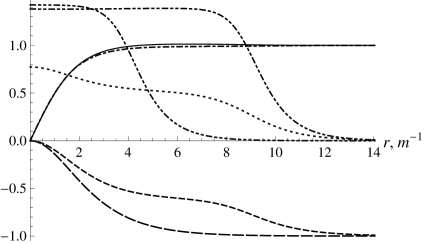
Figure 1: The numerical solution for the dimensionless ansatz functions $m^{-1/2}A_{0}(r)/(er)$ (dotted), $A(r)$ (short-dashed), $F(r)$ (solid), and $m^{-1/2}\sigma(r)$ (dash-dot-dotted) of the vortex-Q-ball system and for the dimensionless ansatz functions $A(r)$ (long-dashed), $F(r)$ (dash-dotted), and $m^{-1/2}\sigma(r)$ (dash-dot-dot-dotted) of the noninteracting vortex and Q-ball. The model’s parameters are the following: $e=q=0.3\,m^{1/2}$, $\lambda=0.173\,m$, $v=1.7\,m^{1/2}$, $g=1.0\,m$, $h=0.26$, and $N=1$. The phase frequency $\omega=0.4\,m$.

Now let us present some numerical results. We use the natural units $c=1$, $\hbar=1$, and the mass $m$ of scalar $\chi$-particle is used as the energy unit. Then the model depends on the six parameters: $e$, $q$, $\lambda$, $v$, $g$, and $h$. Let us choose the following values of these parameters: $e=q=0.3\,m^{1/2}$, $\lambda=0.173\,m$, $v=1.7\,m^{1/2}$, $g=1.0\,m$, and $h=0.26$, where the parameters’ dimensions correspond to the $(2+1)$-dimensional case. Such a choice corresponds to the masses $m_{\phi}=\sqrt{2\lambda}v=1.0\,m$ and $m_{A}=\sqrt{2}ev=0.72\,m$ of the scalar $\phi$-particle and the gauge boson, respectively. Note that the mass ratio $m_{A}/m_{\phi}$ is close to the mass ratio $m_{Z}/m_{H}$ of the Standard model. To check the correctness of numerical solution, Eqs. (20), (34), (39), and (40) were used.

Figure 1 presents the numerical solution for the dimensionless zero component $m^{-1/2}A_{0}(r)/(er)$ of the gauge potential and for the dimensionless ansatz functions $A(r)$, $F(r)$, and $m^{-1/2}\sigma(r)$. The vortex part of the solution is in the topological sector with $N=1$, the phase frequency $\omega$ is equal to $0.4\,m$. Figure 1 also presents the numerical solution for the case $q=0$, whereas the other parameters remain the same. The case $q=0$ corresponds to superimposed but noninteracting vortex and Q-ball. From Fig. 1 it follows that the interaction between the vortex and the Q-ball has a significant effect on the shapes of the ansatz functions $A(r)$ and $\sigma(r)$, while the shape of $F(r)$ does not change significantly.

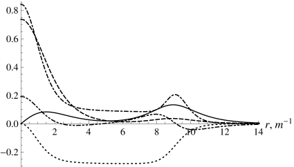
Figure 2: The dimensionless versions of the electric field strength $\tilde{E}_{r}(r)=m^{-3/2}E_{r}(r)$ (solid), the magnetic field strength $\tilde{B}(r)=m^{-3/2}B(r)$ (dashed), the scaled energy density $0.3\,\tilde{\mathcal{E}}(r)=0.3\,m^{-3}\mathcal{E}(r)$ (dash-dotted), the electric charge density $\tilde{j}_{0}(r)=m^{-5/2}j_{0}(r)$ (dash-dot-dotted), and the scaled angular momentum’s density $0.3\,\tilde{\mathcal{J}}(r)=0.3\,m^{-2}\mathcal{J}(r)$ (dotted), corresponding to the solution in Fig. 1.

Figure 2 shows the dimensionless versions of the electric field strength $\tilde{E}_{r}(r)=m^{-3/2}E_{r}(r)$, the magnetic field strength $\tilde{B}(r)=m^{-3/2}B(r)$, the scaled energy density $0.3\,\tilde{\mathcal{E}}(r)=0.3\,m^{-3}\mathcal{E}(r)$, the electric charge density $\tilde{j}_{0}(r)=m^{-5/2}j_{0}(r)$, and the scaled angular momentum’s density $0.3\,\tilde{\mathcal{J}}(r)=0.3\,m^{-2}\mathcal{J}(r)$, corresponding to the solution in Fig. 1. From Fig. 2 it follows that the vortex-Q-ball system can roughly be divided into the three parts: the central transition region, the inner region, and the external transition region. In the inner region, the energy density and the angular momentum’s density are approximately constant, while the electric and magnetic field strengths are close to zero.

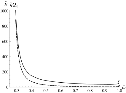
Figure 3: The dependences of the dimensionless soliton energy $\tilde{E}=m^{-1}E$ (solid) and the dimensionless electric charge $\tilde{q}Q_{\chi}=m^{-1/2}qQ_{\chi}$ (dashed) of the scalar field $\chi$ on the dimensionless phase frequency $\tilde{\omega}=m^{-1}\omega$. The model’s parameters are the same as in Fig. 1.

Figure 3 presents the dependences of the dimensionless soliton energy $\tilde{E}=m^{-1}E$ and the dimensionless electric charge $\tilde{q}Q_{\chi}=m^{-1/2}qQ_{\chi}$ of the scalar field $\chi$ on the dimensionless phase frequency $\tilde{\omega}=m^{-1}\omega$. The dependences are presented in the range from the minimum value of $\tilde{\omega}$ to its maximum value of $1$ that we managed to reach by numerical methods. From Fig. 3 it follows that the energy $E$ and the Noether charge $Q_{\chi}$ of the vortex-Q-ball system tend to infinity as $\tilde{\omega}\rightarrow\tilde{\omega}_{\min}$ (thin-wall regime). In the thin-wall regime, the spatial size of the soliton’s inner region increases indefinitely, so the main contribution to the soliton’s energy comes from this region.

In Fig. 4 we can see the dependences that are the same as those in Fig. 3, but are shown in a neighborhood of the maximum value $\tilde{\omega}=1$. From Fig. 4 it follows that the curves $\tilde{E}(\tilde{\omega})$ and $Q_{\chi}(\tilde{\omega})$ consist of two branches. The left branches are finished at $\tilde{\omega}_{-}\approx 0.99404$, whereas the right ones are started at $\tilde{\omega}_{+}\approx 0.99389$. Note that $\tilde{\omega}_{-}>\tilde{\omega}_{+}$ so that the branches are overlapped. It was found numerically that $Q_{\chi}(\tilde{\omega})$ and $\tilde{E}(\tilde{\omega})$ have the following behaviour as $\tilde{\omega}\rightarrow\tilde{\omega}_{\pm}$:

$$Q_{\chi}\underset{\tilde{\omega}\rightarrow\tilde{\omega}_{\pm}}{\longrightarrow}Q_{\chi_{\pm}}\pm 3A_{\pm}\left(\mp\tilde{\omega}_{\pm}\pm\tilde{\omega}\right)^{\frac{1}{3}},$$ (44)

$$\tilde{E}\underset{\tilde{\omega}\rightarrow\tilde{\omega}_{\pm}}{\longrightarrow}\tilde{E}_{\pm}\pm\frac{3}{4}A_{\pm}\left(3\tilde{\omega}_{\pm}+\tilde{\omega}\right)\left(\mp\tilde{\omega}_{\pm}\pm\tilde{\omega}\right)^{\frac{1}{3}},$$

where $A_{\pm}$ are positive constants. Note that the behaviour of $Q_{\chi}(\tilde{\omega})$ and $\tilde{E}(\tilde{\omega})$ in neighborhoods of $\tilde{\omega}_{+}$ and $\tilde{\omega}_{-}$ is in agreement with Eq. (20). From Eq. (44) it follows that the left and right branches have the branch points at $\tilde{\omega}_{-}$ and $\tilde{\omega}_{+}$, respectively. Such behaviour of $Q_{\chi}(\tilde{\omega})$ and $\tilde{E}(\tilde{\omega})$ in a neighborhood of the maximum value $\tilde{\omega}=1$ is very different from that of the two-dimensional Q-ball [7].

Figure 4: The same dependences as those in Fig. 3, but shown in a neighborhood of $\tilde{\omega}=1$.

Figure 5 shows the dependence of the vortex-Q-ball system’s dimensionless energy $\tilde{E}$ on the Noether charge $Q_{\chi}$. It also shows the similar dependence for the two-dimensional Q-ball with the same parameters $m$, $g$, and $h$ as the vortex-Q-ball system, and the straight line $\tilde{E}=Q_{\chi}$. We can see that the two-dimensional Q-ball’s curve $\tilde{E}(Q_{\chi})$ is tangent to the straight line $\tilde{E}=Q_{\chi}$ as it should be [7]. In contrast to this, the vortex-Q-ball system’s curve $\tilde{E}(Q_{\chi})$ has the cusp. Moreover this curve has the gap that corresponds to the jump from the left to the right branches in Fig. 4. From Fig. 5 it follows that the Q-ball component of the the vortex-Q-ball system is stable to the decay in the massive scalar $\chi$-particles in the thin-wall regime.

Figure 5: The dependence of the vortex-Q-ball system’s dimensionless energy $\tilde{E}$ on the Noether charge $Q_{\chi}$ (solid) and that of the two-dimensional Q-ball (dash-dotted) with the same parameters $m$, $g$, and $h$ as the vortex-Q-ball system. The dotted line is the straight line $\tilde{E}=Q_{\chi}$.

5 Conclusions

In the present paper, the soliton system consisting of a vortex and a Q-ball interacting through a common Abelian gauge field has been researched. This two-dimensional system is electrically neutral since only the Maxwell gauge term is presented in the Lagrangian (1). Nevertheless, the vortex-Q-ball system possesses a nonzero radial electric field. Moreover, this system also has a quantized magnetic flux. As a result, the soliton system possesses a nonzero angular momentum that turns out to be proportional to the Noether charge of the scalar $\phi$- or $\chi$-field. The vortex-Q-ball system combines properties of nontopological solitons (Eq. (20)) and those of topological solitons (topological boundary condition (27) for $A(r)$ and, as consequence, magnetic flux quantization (28)). Finally, the interaction between the vortex and the Q-ball leads to the significant change of the vortex-Q-ball system’s dependence $E(Q_{\chi})$ in comparison with that of the two-dimensional Q-ball.

It should be noted that in $(2+1)$ dimensions, in addition to the ordinary Lorentz-invariant Maxwell term, there exists a Lorentz-invariant Chern-Simons term, which can be included in Lagrangians of gauge models [8, 9, 10]. In the presence of this term, the model’s gauge field becomes topologically massive, thus making possible the existence of two-dimensional solitons that have a nonzero quantized electric charge [5, 11, 12, 13, 14, 15]. Due to the presence of electric and magnetic fields, these solitons also possess nonzero angular momentums that satisfy the relations similar to Eq. (39).

References

• [1] A. A. Abrikosov, Sov. Phys. JETP 5 (1957) 1174.
• [2] H. B. Nielsen, P. Olesen, Nucl. Phys. B 61 (1973) 45.
• [3] A. A. Belavin, A. M. Polyakov, JETP Lett. 22 (1975) 245.
• [4] J. Gladikowski, B. M. A. G. Piette, B. J. Schroers, Phys. Rev. D 53 (1996) 844.
• [5] J. Hong, Y. Kim, P. Y. Pac, Phys. Rev. Lett. 64 (1990) 2230.
• [6] S. Coleman, Nucl. Phys. B 262 (1985) 263.
• [7] T. D. Lee, Y. Pang, Phys. Rep. 221 (1992) 251.
• [8] R. Jackiw, S. Templeton, Phys. Rev. D 23 (1981) 2291.
• [9] J. F. Schonfeld, Nucl. Phys. B 185 (1981) 157.
• [10] S. Deser, R. Jackiw, S. Templeton, Phys. Rev. Lett. 48 (1982) 975.
• [11] S. K. Paul, A. Khare, Phys. Lett. B 174 (1986) 420.
• [12] S. K. Paul, A. Khare, Phys. Lett. B 177 (1986) 453.
• [13] P. K. Ghosh, S. K. Ghosh, Phys. Lett. B 366 (1996) 199.
• [14] R. Jackiw, E. J. Weinberg, Phys. Rev. Lett. 64 (1990) 2234.
• [15] R. Jackiw, K. Lee, E. J. Weinberg, Phys. Rev. D 42 (1990) 3488.