Integrating Sub-6 GHz and Millimeter Wave to Combat Blockage: Delay-Optimal Scheduling

Guidan Yao1, Morteza Hashemi2, and Ness B. Shroff 13 1 Department of Electrical and Computer Engineering, Ohio State University 2Department of Electrical Engineering and Computer Science, University of Kansas (KU) 3Department of Computer Engineering and Computer Science, Ohio State University
Abstract

Millimeter wave (mmWave) technologies have the potential to achieve very high data rates, but suffer from intermittent connectivity. In this paper, we provision an architecture to integrate sub-6 GHz and mmWave technologies, where we incorporate the sub-6 GHz interface as a fallback data transfer mechanism to combat blockage and intermittent connectivity of the mmWave communications. To this end, we investigate the problem of scheduling data packets across the mmWave and sub-6 GHz interfaces such that the average delay of system is minimized. This problem can be formulated as Markov Decision Process. We first investigate the problem of discounted delay minimization, and prove that the optimal policy is of the threshold-type, i.e., data packets should always be routed to the mmWave interface as long as the number of packets in the system is smaller than a threshold. Then, we show that the results of the discounted delay problem hold for the average delay problem as well. Through numerical results, we demonstrate that under heavy traffic, integrating sub-6 GHz with mmWave can reduce the average delay by up to 70%. Further, our scheduling policy substantially reduces the delay over the celebrated MaxWeight policy.

I Introduction

The annual amount of mobile data is projected to surpass 130 exabits by 2020 [1]. With such rapid increases in mobile data traffic, we are facing unprecedented challenges due to the shortage of wireless spectrum. To mitigate the problem of spectrum scarcity, the millimeter wave (mmWave) band, ranging from 30 GHz to 300 GHz, provides a promising solution [2]. However, before mmWave communications can become a reality, there exist several significant challenges that need to be overcome. In particular, mmWave channels can be highly variable with intermittent on-off periods. Due to small wavelengths in the mmWave band, most objects, such as concrete walls, a human body or even rain drops, may cause blocking and reflections as opposed to scattering and diffraction in the sub-6 GHz frequencies. In this case, blockage may completely break the mmWave link and result in an almost zero delivery rate [3, 4, 5]. In the provisioned applications of mmWave, human blockage is one of the main challenges that can increase the path loss by more than 20 dB [6, 7, 8, 9].

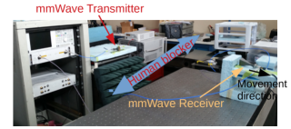
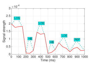
To demonstrate the effect of human blockage on mmWave links, we have conducted a set of measurements with a stationary transmitter and a mobile receiver that moves away from the transmitter with the speed of 1 m/s. During the time intervals 200300200300200-300 and 500600500600500-600 ms, a human body blocks the line-of-sight (LOS) path between the transmitter and receiver. Figure 1 shows our basic experimental setup and Fig. 2 depicts the strength of received signal at the mobile receiver over time [10]. From the results, we see that the received signal strength falls to almost zero under blockage, which can be modeled as an OFF or unavailable period. Therefore, the mmWave link exhibits an ON/OFF connectivity pattern under blockage scenarios such that during the OFF periods, delivery rate and delay performance can highly degrade.
Refer to caption
Figure 1: Measurement setup and experiment scenario to investigate the effect of human blockage on mmWave channels.
Refer to caption
Figure 2: Received mmWave signal strength under line of sight (LOS), human blocker (HB), and reflection (REF) [10].

In order to mitigate the effects of intermittent connectivity, especially for delay-sensitive applications, several methods have been proposed. For instance, the authors in [5] and [11] exploit reflection paths and multi-hop paths to combat blockage. These methods are reactive in the sense that the search for an alternative path is triggered after blockage occurs. However, since the link speed of the mmWave interface (multi-Gbps) is comparable to the speed at which a typical processor in a smart device operates, these methods may not be able to track and respond to channel variations in real-time. Therefore, it necessitates the use of a reasonably large buffer at the mmWave interface along with proactive solutions to complement this design. In addition to the aforementioned methods, there exist several works on integrating the mmWave and sub-6 GHz technologies. For instance, due to spatial correlation, information of the sub-6 GHz channel can be extracted to reduce mmWave beamforming overhead [12, 13], while [14] uses an online learning method to enhance beamforming delay. Moreover, the authors in [15, 10, semiari2017joint] consider resource allocation and cooperative communication between the sub-6 GHz and mmWave to maximize either the throughput of the system or the quality-of-service per user application.

Although an integrated mmWave/sub-6 GHz architecture has been previously proposed, the delay minimization problem in this integrated architecture has not been explored yet. In particular, we raise the following questions that: Would the system delay benefit from the sub-6 GHz interface? If so, when should the sub-6 interface be used so that the delay of the system is minimized? In this paper, we exploit the sub-6 GHz interface as a fallback data transfer mechanism, and investigate the problem of delay-optimal scheduling across the sub-6 GHz and mmWave interfaces. We develop a proactive scheduling policy that is expressed in terms of the queue length of the mmWave and sub-6 GHz interfaces.

In order to obtain a delay-optimal policy, we first consider minimizing the expected total discounted delay. We obtain three rules for the delay-optimal scheduling using value iteration in Markov Decision Process (MDP). Next, we collapse our system state space from four dimension to three dimension, and further demonstrate that the optimal policy for the discounted delay problem is of a threshold-type. Finally, we extend our results to the average delay problem. Through simulations, we show that it is important to use the sub-6 GHz interface especially when the mmWave is unavailable with high probability and confirm that such a threshold-type policy improves the average delay performance while achieving similar throughput performance as the throughput-optimal and well-studied MaxWeight policy [23].

In summary, our main contributions are as follows: (i) we formulate the discounted delay optimality problem in the integrated sub-6 GHz/mmWave architecture as an MDP and provide partial characteristics of the optimal policy. Based on the findings, we propose a threshold-type policy and then prove its optimality; (ii) we further show that the proposed policy is also optimal for the average delay problem; and (iii) we provide a methodology for solving the delay minimization problem in settings consisting of tandem and parallel queues with heterogeneous servers.

We use the following notations throughout the paper. Non-bold lowercase and uppercase letters are used for scalers and sets, respectively. Bold lowercase letters are used for vectors. In addition, 𝔼[.]\mathds{E}[.] denotes the expectation operator. The sub-6 GHz and mmWave variables are denoted by ()sub-6subscriptsub-6\left(\cdot\right)_{\text{sub-6}} and ()mmsubscriptmm\left(\cdot\right)_{\text{mm}}, respectively.

II Related Work

In order to mitigate the effects of blockers and intermittent mmWave links, there have been several works to provide reliable communication over the mmWave band. In [5], the authors utilized reflections from walls or reflectors to assist directional paths. However, the behavior of the reflectors depends on the relative placement of transmitter/receiver to reflectors (e.g., incident angle). In addition, there is an additional reflection loss incurred due to reflectors. In [fonseca2006collection], a spatial diversity technique was utilized to combat blockage caused by human movement. The technique delivers the same packets through several propagation paths simultaneously instead of the strongest path. Although this method can mitigate the effect of blockage, it increases energy consumption. The authors in [singh2009blockage] devised a multi-hop directional MAC protocol for mmWave indoor wireless personal area networks. The key idea is to go around the obstacle through multi-hop paths. Directional MAC protocol is also studied in [4] where the authors investigate a joint optimization over relay selection and spatial reuse so that network performance could be improved. This method is limited to two-hop relaying.

In another related line of research, the slow-server problem, in which the goal is to obtain a delay optimal scheduling policy in a queuing system with heterogeneous (i.e., fast and slow) servers, has been studied. In that scenario, the main question that has been answered is: should the slow server be laid aside or utilized occasionally? The focus of this problem is the trade-off between waiting in queue and entering slow servers when fast servers are busy or unavailable. In this context, the mmWave link acts as the fast server that becomes unavailable if blockage occurs. The authors in [16] presented a M/M/2 queuing system with two heterogeneous servers and conjectured that the optimal policy for minimizing the average delay and expected total discounted delay in system is of the threshold-type. The conjecture was later confirmed in [17]. Following this work, [20] extended the result to the system with multi-servers (i.e., more than two), and [22] studied the delay minimization problem with different arrival and service processes. Our delay minimization problem differs from the aforementioned works in two key aspects:

  1. 1.

    In our system architecture (see Fig. 3 and Fig. 4), packets that are scheduled to the mmWave link have to first go through a processing server for essential data processing. This makes our system a mix of the tandem and parallel queues. Further, the processing server and the mmWave queue constitute a tandem queue which is part of parallel queues. In this case, to prove optimality of the proposed threshold-type policy, we need to show the relationship between the resulting delays starting at states with the packet in processing server and the packet moved to the mmWave queue, where the two states cannot be collapsed. This makes the problem more complex than the traditional slow server problem.

  2. 2.

    Our mmWave interface includes both a server and a buffer, which together constitute the mmWave queue. In addition, we require packets in the mmWave queue to be impatient, meaning that packets can be reneged to sub-6 GHz for service. Note that the packets in the sub-6 GHz server cannot be sent back to the mmWave queue or the head buffer. Adding the flexibility of reneging to the mmWave packets introduces several new challenges such as: should packets be routed from the mmWave queue or the head buffer to the sub-6 GHz queue? Therefore, in addition to the trade-off between waiting in the head queue (entrance to the system) and entering the slow server which is investigated in the slow-server problem, our problem also considers the trade-off between waiting in the mmWave queue and entering the slow server and trade-off between dispatching packets from the head buffer and the mmWave queue.

III Problem Setup

In this section, we present the system model and formulate the delay minimization problem.

III-A System Model

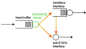
We consider an integrated communication architecture with dual sub-6 GHz and mmWave interfaces as shown in Fig. 3. The infinite head buffer is utilized to store all packets waiting to be processed and served by either mmWave or sub-6 GHz. The processing server is responsible for essential data processing before scheduling. Plus, the system includes two servers (mmWave and sub-6 GHz servers) with extremely different service rate, i.e. the service rate of mmWave can be 100 times larger than the service rate of sub-6 GHz.

(i) Queue Models: In our system model, we add a buffer to the mmWave server, which stores packets routed from the head buffer. The rationality of our design (i.e., a separate queue for the mmWave interface) is described next. The service rate of the mmWave server is comparable to the processing server (i.e., processor speed). Moreover, mmWave is very sensitive to blockage, which is hard to quickly predict. If we assume that there is no buffer for the mmWave server, then every packet needs to wait in the head queue util the mmWave server is available. In the case, the packet will experience service time of both the processing and the mmWave servers (almost double the service time of the mmWave) except waiting time in the head buffer. Then, the performance of mmWave is degraded by approximately half. On the contrary, if the mmWave server has its own buffer for processed packets, part of waiting time in the head buffer can be utilized to process packets in advance, which reduces the experienced service time mentioned above. However, the sub-6 GHz link is much slower than the processing server. Therefore, processing delay can be ignored compared to service time of the sub-6 GHz. In other words, it is not necessary for the sub-6 GHz server to have its own buffer considering the cost of buffer. Thus, it is appropriate to assume that the sub-6 GHz interface acts as a server with a buffer size of one, while the mmWave interface consists of an infinite buffer and a server.
Refer to caption
Figure 3: Integrated sub-6 GHz and mmWave architecture.

(ii) Two-state mmWave link; Available or Unavailable: As mentioned before, the mmWave link is highly variable with intermittent ON-OFF periods. It is reasonable to model the mmWave service rate with two states, say available and unavailable. For the unavailable state, the mmWave channel is almost disconnected and thus we assume that the service rate of the mmWave is 0. For the available state, we assume that the service time is exponentially distributed with parameter μmmsubscript𝜇mm\mu_{\text{mm}}. Further, we denote the probability of available and unavailable states with pasubscript𝑝ap_{\text{a}} and pnasubscript𝑝nap_{\text{na}}, respectively.

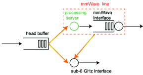
We further assume that arrivals to the system form a Poisson process with parameter λ𝜆\lambda, and that service times of the processing server and the sub-6 GHz interface are exponentially distributed with parameter μpsubscript𝜇p\mu_{\text{p}} and μsub-6subscript𝜇sub-6\mu_{\text{sub-6}}, respectively. Given that the mmWave service rate is of the same order as the clock speed of the processor (i.e., several GHz), we assume that μpsubscript𝜇p\mu_{\text{p}} is much faster than μsub-6subscript𝜇sub-6\mu_{\text{sub-6}} but in the same order as μmmsubscript𝜇mm\mu_{\text{mm}}. Since delay of the processing server becomes negligible compared with the sub-6 GHz interface, we consider the equivalent model depicted in Fig. 4 where we call the processing server and mmWave interface as mmWave line.

Within this content, we further clarify the difference of our problem from previous work, which has been briefly discussed in Section II. In Fig. 3, packets that are scheduled to the mmWave line have to go through a processing server first. These make our system a mix of the tandem and parallel queues. In the case, to finally obtain the optimality of the proposed threshold-type policy, we need to show the relationship between the resulting delays starting at states with the packet in processing server and the packet moved to the mmWave queue, where the two states cannot be collapsed at this step. This implies that our problem is more complex than the classic slow server problem.
Refer to caption
Figure 4: Equivalent system model.

As mentioned in Section II, to avoid a large waiting time in the mmWave queue due to intermittent channel (e.g., due to blockage), we require the packets to be impatient in the sense that if the waiting time of the head-of-line packet in the mmWave queue becomes large, the packet “reneges” (is moved to) from the mmWave line or “routes” from the head buffer (is dispatched to) to the sub-6 GHz interface. Note that the packet in the sub-6 GHz server cannot be sent back to the mmWave line or the head buffer. Adding the reneging concept introduces new challenges such as : should the packets be moved from the head buffer or the mmWave queue to the sub-6 GHz server? Therefore, in addition to the trade-off between waiting in the head queue and entering the slow server which is investigated in the slow-server problem, our problem investigates: (i) the trade-off between waiting in the mmWave line and entering the slow server, and (ii) trade-off between dispatching packets from the head buffer and the mmWave line.

III-B System Dynamics

(i) System States: Let q0subscript𝑞0q_{0}, q1subscript𝑞1q_{1} absent\in\mathbb{N} denote the queue length of the head buffer and mmWave interface, respectively. Moreover, l1subscript𝑙1l_{1}, l2subscript𝑙2l_{2} {0,1}absent01\in\{0,1\} denote the busy/idle condition of the processing server and sub-6 GHz interface, respectively. In this case, l1=1subscript𝑙11l_{1}=1 implies a busy server. Therefore, the system state can be expressed by a four-dimensional vector 𝐪(q0,l1,q1,l2)𝐪subscript𝑞0subscript𝑙1subscript𝑞1subscript𝑙2\mathbf{q}\triangleq\left(q_{0},l_{1},q_{1},l_{2}\right) with the state space of Q×{0,1}××{0,1}𝑄0101Q\triangleq\mathbb{N}\times\{0,1\}\times\mathbb{N}\times\{0,1\}.

(ii) Events: There are four different events that happen in the system, which are defined as follows:

(1) Arrival of a packet to the head buffer: After arrival of one packet, state of the system is changed as follows:

𝒜0(𝐪)(q0+1,l1,q1,l2).subscript𝒜0𝐪subscript𝑞01subscript𝑙1subscript𝑞1subscript𝑙2\displaystyle\mathcal{A}_{0}\left(\mathbf{q}\right)\triangleq\left(q_{0}+1,l_{1},q_{1},l_{2}\right).

(2) Departure of a packet from the mmWave interface: The departure of a packet from the mmWave queue changes the system state as

𝒟1(𝐪)(q0,l1,(q11)+,l2),subscript𝒟1𝐪subscript𝑞0subscript𝑙1superscriptsubscript𝑞11subscript𝑙2\displaystyle\mathcal{D}_{1}\left(\mathbf{q}\right)\triangleq\left(q_{0},l_{1},\left(q_{1}-1\right)^{+},l_{2}\right),

where ()+=max(,0).superscript0\left(\cdot\right)^{+}=\max\left(\cdot,0\right).

(3) Departure of a packet from the sub-6 GHz interface: If a packet departs from the sub-6 GHz queue, state of the system changes as

𝒟2(𝐪)(q0,l1,q1,(l21)+).subscript𝒟2𝐪subscript𝑞0subscript𝑙1subscript𝑞1superscriptsubscript𝑙21\displaystyle\mathcal{D}_{2}\left(\mathbf{q}\right)\triangleq\left(q_{0},l_{1},q_{1},\left(l_{2}-1\right)^{+}\right).

(4) Processing completion: If the processing server delivers a packet to the mmWave queue, the system state changes as

𝒯(𝐪)(q0,(l11)+,l1+q1,l2).𝒯𝐪subscript𝑞0superscriptsubscript𝑙11subscript𝑙1subscript𝑞1subscript𝑙2\displaystyle\mathcal{T}\left(\mathbf{q}\right)\triangleq\left(q_{0},\left(l_{1}-1\right)^{+},l_{1}+q_{1},l_{2}\right).

Note that we introduce “dummy” packets for the last three events when q1=0subscript𝑞10q_{1}=0, l2=0subscript𝑙20l_{2}=0 and l1=0subscript𝑙10l_{1}=0, respectively. This is further elaborated in Section III-C.

(iii) Actions: K={Ah,A1,A2,Ab,Ar}𝐾subscript𝐴subscript𝐴1subscript𝐴2subscript𝐴𝑏subscript𝐴𝑟K=\{A_{h},A_{1},A_{2},A_{b},A_{r}\} is an action set. K𝐪Ksubscript𝐾𝐪𝐾K_{\mathbf{q}}\subseteq K denotes the set of admissible actions in state 𝐪𝐪\mathbf{q}. Each action in set K𝐾K is defined as follows:

(1) Holding: Action Ahsubscript𝐴A_{h} keeps the system state unchanged, and is defined on Q𝑄Q. Therefore, we have

Ah(𝐪)(q0,l1,q1,l2).subscript𝐴𝐪subscript𝑞0subscript𝑙1subscript𝑞1subscript𝑙2A_{h}\left(\mathbf{q}\right)\triangleq\left(q_{0},l_{1},q_{1},l_{2}\right).

(2) Scheduling-on-mmWave: A packet can be routed to the mmWave line if the processing server is idle, i.e.,

A1(𝐪)(q01,1,q1,l2),subscript𝐴1𝐪subscript𝑞011subscript𝑞1subscript𝑙2A_{\text{1}}\left(\mathbf{q}\right)\triangleq\left(q_{0}-1,1,q_{1},l_{2}\right),

which is defined on the set {𝐪q01,l1=0}conditional-set𝐪formulae-sequencesubscript𝑞01subscript𝑙10\{\mathbf{q}\mid q_{0}\geq 1,l_{1}=0\}.

(3) Scheduling-on-sub-6: A packet can be routed to the sub-6 GHz interface if the sub-6 GHz server is idle, i.e.,

A2(𝐪)(q01,l1,q1,1),subscript𝐴2𝐪subscript𝑞01subscript𝑙1subscript𝑞11A_{2}\left(\mathbf{q}\right)\triangleq\left(q_{0}-1,l_{1},q_{1},1\right),

which is defined on the set {𝐪q01,l2=0}conditional-set𝐪formulae-sequencesubscript𝑞01subscript𝑙20\{\mathbf{q}\mid q_{0}\geq 1,l_{2}=0\}.

(4) Scheduling-on-both: Action Absubscript𝐴𝑏A_{b} dispatches two packets to the sub-6 GHz and processing servers simultaneously, i.e.,

Ab(𝐪)(q02,1,q1,1),subscript𝐴𝑏𝐪subscript𝑞021subscript𝑞11A_{b}\left(\mathbf{q}\right)\triangleq\left(q_{0}-2,1,q_{1},1\right),

which is defined on the set {𝐪q02,l1=l2=0}conditional-set𝐪formulae-sequencesubscript𝑞02subscript𝑙1subscript𝑙20\{\mathbf{q}\mid q_{0}\geq 2,l_{1}=l_{2}=0\}.

(5) Reneging: Action Arsubscript𝐴𝑟A_{r} moves a packet from the mmWave line to the sub-6 GHz interface, and it is defined on the set {𝐪q1+l11,l2=0}conditional-set𝐪formulae-sequencesubscript𝑞1subscript𝑙11subscript𝑙20\left\{\mathbf{q}\mid q_{1}+l_{1}\geq 1,l_{2}=0\right\}. Let Arpsubscript𝐴subscript𝑟pA_{r_{\text{p}}} and Armmsubscript𝐴subscript𝑟mmA_{r_{\text{mm}}} denote the reneging actions from the processing server and mmWave interface, respectively. Therefore, we have

Arp(𝐪)(q0,0,q1,1),𝐪{𝐪l1=1,l2=0};Armm(𝐪)(q0,l1,q11,1),𝐪{𝐪q11,l2=0}.subscript𝐴subscript𝑟p𝐪subscript𝑞00subscript𝑞11𝐪conditional-set𝐪formulae-sequencesubscript𝑙11subscript𝑙20subscript𝐴subscript𝑟mm𝐪subscript𝑞0subscript𝑙1subscript𝑞111𝐪conditional-set𝐪formulae-sequencesubscript𝑞11subscript𝑙20\displaystyle\begin{array}[]{l l}A_{r_{\text{p}}}\left(\mathbf{q}\right)\triangleq\left(q_{0},0,q_{1},1\right),&\mathbf{q}\in\{\mathbf{q}\mid l_{1}=1,\,l_{2}=0\};\\ A_{r_{\text{mm}}}\left(\mathbf{q}\right)\triangleq\left(q_{0},l_{1},q_{1}-1,1\right),&\mathbf{q}\in\{\mathbf{q}\mid q_{1}\geq 1,\,l_{2}=0\}.\end{array} (3)

Then, the reneging action Arsubscript𝐴𝑟A_{r} is expressed as

Ar(𝐪){Arp(𝐪)ifl1=1,q1=0Armm(𝐪)ifl1=0,q11argminAa{Arp,Armm}v(Aa(𝐪))otherwisesubscript𝐴𝑟𝐪casessubscript𝐴subscript𝑟p𝐪formulae-sequenceifsubscript𝑙11subscript𝑞10subscript𝐴subscript𝑟mm𝐪formulae-sequenceifsubscript𝑙10subscript𝑞11subscriptargminsubscript𝐴𝑎subscript𝐴subscript𝑟psubscript𝐴subscript𝑟mm𝑣subscript𝐴𝑎𝐪otherwise\displaystyle A_{r}\left(\mathbf{q}\right)\triangleq\left\{\begin{array}[]{l l}A_{r_{\text{p}}}\left(\mathbf{q}\right)&\text{if}\,\,l_{1}=1,\,\,q_{1}=0\\ A_{r_{\text{mm}}}\left(\mathbf{q}\right)&\text{if}\,\,l_{1}=0,\,\,q_{1}\geq 1\\ \mathop{\operatorname*{arg\,min}}\limits_{A_{a}\in\{A_{r_{\text{p}}},A_{r_{\text{mm}}}\}}v\left(A_{a}\left(\mathbf{q}\right)\right)&\text{otherwise}\end{array}\right. (7)

where v()𝑣v\left(\cdot\right) denotes the delay cost. Note that if Arpsubscript𝐴subscript𝑟pA_{r_{\text{p}}} and Armmsubscript𝐴subscript𝑟mmA_{r_{\text{mm}}} are admissible, we select an action that results in a smaller cost. In Section IV, we show that Ar=Arpsubscript𝐴𝑟subscript𝐴subscript𝑟pA_{r}=A_{r_{\text{p}}} for the discounted delay problem when both Arpsubscript𝐴subscript𝑟pA_{r_{\text{p}}} and Armmsubscript𝐴subscript𝑟mmA_{r_{\text{mm}}} are admissible.

III-C Problem Formulation

Average Delay Problem: Our objective is to schedule packets across the mmWave and sub-6 GHz interfaces such that the average delay of system is minimized. To this end, we know that, by Little’s Law, the average delay minimization problem is equivalent to minimizing the average total number of packets in the system, which is expressed as follows:

minπΠlim supT1T𝔼π[t=1T(𝐪[t]𝐞)𝑑t],subscript𝜋Πsubscriptlimit-supremum𝑇1𝑇superscript𝔼𝜋delimited-[]superscriptsubscript𝑡1𝑇𝐪delimited-[]𝑡𝐞differential-d𝑡\min_{\pi\in\Pi}\,\,\limsup_{T\to\infty}\frac{1}{T}\mathbb{E}^{\pi}\left[\int_{t=1}^{T}\left(\mathbf{q}[t]\cdot\mathbf{e}\right)dt\right], (8)

where 𝔼πsuperscript𝔼𝜋\mathbb{E}^{\pi} denotes the conditional expectation given policy π𝜋\pi, 𝐪[t]Q𝐪delimited-[]𝑡𝑄\mathbf{q}[t]\in Q is the system state at time t𝑡t, ΠΠ\Pi denotes the set of all admissible policies, and 𝐞=(1,1,1,1)T𝐞superscript1111T\mathbf{e}=\left(1,1,1,1\right)^{\text{T}}. We model the system evolution as an MDP, and for simplicity, we convert the continuous-time MDP problem into an equivalent discrete-time MDP problem with the method of uniformization [24]. In particular, we assume that all servers will serve “dummy” packets whenever they are idle. Then, we separate continuous time into time slots with sequences when either a packet arrival or a packet (real or dummy) departure from the processing server or interfaces happens. Let N={1,2,3,}𝑁123N=\{1,2,3,\cdots\} denote the set of time slots such that the channel state does not change during each time slot. Then, the system state at the n𝑛n-th time slot is expressed as 𝐪[n]𝐪delimited-[]𝑛\mathbf{q}[n]. Furthermore, without loss of generality, we scale time and assume that λ+μp+paμmm+μsub-6=1𝜆subscript𝜇psubscript𝑝asubscript𝜇mmsubscript𝜇sub-61\lambda+\mu_{\text{p}}+p_{\text{a}}\mu_{\text{mm}}+\mu_{\text{sub-6}}=1.

We consider the set of control variables U{(u0,u1,u2,u3)u0,u1,u2,u3K}𝑈conditional-setsubscript𝑢0subscript𝑢1subscript𝑢2subscript𝑢3subscript𝑢0subscript𝑢1subscript𝑢2subscript𝑢3𝐾U\triangleq\{(u_{0},u_{1},u_{2},\\ u_{3})\mid u_{0},u_{1},u_{2},u_{3}\in K\}. Then, the decision rule at the n𝑛n-th decision epoch (the beginning of the n𝑛n-th time slot) is a mapping from the system states to the control variables, i.e., dn:QU:subscript𝑑𝑛𝑄𝑈d_{n}:Q\rightarrow U, for all nN𝑛𝑁n\in N and the policy π𝜋\pi is a sequence of the decision rules, i.e., π=(d1,d2,)𝜋subscript𝑑1subscript𝑑2\pi=\left(d_{1},d_{2},\cdots\right). Further, if 𝐪[n]=𝐪𝐪delimited-[]𝑛superscript𝐪\mathbf{q}\left[n\right]=\mathbf{q^{\prime}} and dn(𝐪)=(u0,u1,u2,u3)subscript𝑑𝑛superscript𝐪subscript𝑢0subscript𝑢1subscript𝑢2subscript𝑢3d_{n}\left(\mathbf{q^{\prime}}\right)=\left(u_{0},u_{1},u_{2},u_{3}\right) for certain nN𝑛𝑁n\in N, then if an arrival occurs at the (n+1)𝑛1(n+1)-th epoch, we would take actions according to u0subscript𝑢0u_{0}. Similar explanation applies to u1subscript𝑢1u_{1}, u2subscript𝑢2u_{2}, u3subscript𝑢3u_{3}. Thus, the transition probabilities in the discrete-time MDP are expressed as

(𝐪𝐪,𝐮)={λif𝐪=u0(𝒜0(𝐪))μpif𝐪=u1(𝒯(𝐪))paμmmif𝐪=u2(𝒟1(𝐪))μsub-6if𝐪=u3(𝒟2(𝐪))conditionalsuperscript𝐪𝐪𝐮cases𝜆ifsuperscript𝐪subscript𝑢0subscript𝒜0𝐪subscript𝜇pifsuperscript𝐪subscript𝑢1𝒯𝐪subscript𝑝asubscript𝜇mmifsuperscript𝐪subscript𝑢2subscript𝒟1𝐪subscript𝜇sub-6ifsuperscript𝐪subscript𝑢3subscript𝒟2𝐪\displaystyle\mathbb{P}\left(\mathbf{q}^{\prime}\mid\mathbf{q},\mathbf{u}\right)=\begin{cases}\lambda&\text{if}\,\,\,\mathbf{q}^{\prime}=u_{0}\left(\mathcal{A}_{0}\left(\mathbf{q}\right)\right)\\ \mu_{\text{p}}&\text{if}\,\,\,\mathbf{q}^{\prime}=u_{1}\left(\mathcal{T}\left(\mathbf{q}\right)\right)\\ p_{\text{a}}\mu_{\text{mm}}&\text{if}\,\,\,\mathbf{q}^{\prime}=u_{2}\left(\mathcal{D}_{1}\left(\mathbf{q}\right)\right)\\ \mu_{\text{sub-6}}&\text{if}\,\,\,\mathbf{q}^{\prime}=u_{3}\left(\mathcal{D}_{2}\left(\mathbf{q}\right)\right)\\ \end{cases}\vspace{-0.2cm}

Then, with the discrete-time MDP, the uniformized problem is formulated as follows:

minπΠlim supN1N𝔼π[n=1N𝐪[n]𝐞].subscript𝜋Πsubscriptlimit-supremum𝑁1𝑁superscript𝔼𝜋delimited-[]superscriptsubscript𝑛1𝑁𝐪delimited-[]𝑛𝐞\vspace{-0.05cm}\min_{\pi\in\Pi}\,\,\limsup_{N\to\infty}\frac{1}{N}\mathbb{E}^{\pi}\left[\sum_{n=1}^{N}\mathbf{q}[n]\cdot\mathbf{e}\right].\vspace{-0.05cm} (9)

Discounted Delay Problem: To solve the average delay problem, we first consider the problem of minimizing the expected total discounted delay of the system (discounted delay problem) to avoid convergence issues in the presence of bounded value function [24]. Next, we extend our results to the average delay problem. The discounted delay problem in the equivalent discrete-time MDP is expressed as

minπΠ𝔼π[n=1βn1𝐪[n]𝐞],subscript𝜋Πsuperscript𝔼𝜋delimited-[]superscriptsubscript𝑛1superscript𝛽𝑛1𝐪delimited-[]𝑛𝐞\min_{\pi\in\Pi}\,\,\,\,\,\mathbb{E}^{\pi}\left[\sum_{n=1}^{\infty}\beta^{n-1}\mathbf{q}[n]\cdot\mathbf{e}\right], (10)

where β𝛽\beta is a discount factor such that 0β<10𝛽10\leq\beta<1. To solve the discounted delay problem, it is known that there exists an optimal deterministic stationary policy [24]. Thus, we only need to consider the class of deterministic stationary policies. We apply the value iteration method to find the optimal policy.

Under the assumption that the system is stable, value (delay) functions of the initial state 𝐪Q𝐪𝑄\mathbf{q}\in Q are bounded real-valued functions. Let V𝑉V denote the Banach space of bounded real-valued functions on Q𝑄Q with supremum norm. Define operator :VV:𝑉𝑉\mathcal{L}:V\rightarrow V as

\IEEEeqnarraymulticol3l(v)(𝐪)\IEEEeqnarraymulticol3𝑙𝑣𝐪\displaystyle\IEEEeqnarraymulticol{3}{l}{\left(\mathcal{L}v\right)\left(\mathbf{q}\right)}
\displaystyle\triangleq 𝐪𝐞+βmin𝐮U𝐪{λv(u0(𝒜0(𝐪)))+μpv(u1(𝒯(𝐪)))\displaystyle\mathbf{q}\cdot\mathbf{e}+\beta\min_{\mathbf{u}\in U_{\mathbf{q}}}\bigg{\{}\lambda v\big{(}u_{0}\left(\mathcal{A}_{0}\left(\mathbf{q}\right)\right)\big{)}+\mu_{\text{p}}v\big{(}u_{1}\left(\mathcal{T}\left(\mathbf{q}\right)\right)\big{)} (11)
+μmmpav(u2(𝒟1(𝐪)))+μsub-6v(u3(𝒟2(𝐪)))},\displaystyle+\mu_{\text{mm}}p_{\text{a}}v\big{(}u_{2}\left(\mathcal{D}_{1}\left(\mathbf{q}\right)\right)\big{)}+\mu_{\text{sub-6}}v\big{(}u_{3}\left(\mathcal{D}_{2}\left(\mathbf{q}\right)\right)\big{)}\bigg{\}},

where v()V𝑣𝑉v\left(\cdot\right)\in V and U𝐪subscript𝑈𝐪U_{\mathbf{q}} denotes the set of admissible control variables in state 𝐪𝐪\mathbf{q} such that U𝐪Usubscript𝑈𝐪𝑈U_{\mathbf{q}}\subseteq U. Let Jβ(𝐪)subscript𝐽𝛽𝐪J_{\beta}\left(\mathbf{q}\right) denote optimal expected total discounted delay function of initial state 𝐪𝐪\mathbf{q}. Then, Jβ(𝐪)subscript𝐽𝛽𝐪J_{\beta}\left(\mathbf{q}\right) is a solution of Bellman function, i.e., Jβ(𝐪)=Jβ(𝐪)subscript𝐽𝛽𝐪subscript𝐽𝛽𝐪J_{\beta}\left(\mathbf{q}\right)=\mathcal{L}J_{\beta}\left(\mathbf{q}\right).

IV Delay Optimal Policy

IV-A Discounted Delay Problem

Except that the mmWave channel is extremely intermittent, the average service rate of the mmWave is much higher than the sub-6 GHz (e.g., two orders of magnitude). Besides, the service rate of the mmWave and processing server are in the same order. Hence, it is reasonable to assume that the expected time for a packet to go through empty mmWave line is less than empty sub-6 GHz interface, i.e., 1paμmm+1μp<1μsub-61subscript𝑝asubscript𝜇mm1subscript𝜇p1subscript𝜇sub-6\frac{1}{p_{\text{a}}\mu_{\text{mm}}}+\frac{1}{\mu_{\text{p}}}<\frac{1}{\mu_{\text{sub-6}}}. With this assumption, we have the following theorem:

Theorem 1.

Assuming that 1paμmm+1μp<1μsub-61subscript𝑝asubscript𝜇mm1subscript𝜇p1subscript𝜇sub-6\frac{1}{p_{\text{a}}\mu_{\text{mm}}}+\frac{1}{\mu_{\text{p}}}<\frac{1}{\mu_{\text{sub-6}}}, then we have

(a)Jβ(A1(𝐪))Jβ(Ah(𝐪))ifq01,l1=0;(b)Jβ(A2(𝐪))Jβ(Ar(𝐪))ifq01,l1+q11,andl2=0;(c)Jβ(𝒯(𝐪))Jβ(𝐪)ifl1=1;(d)Jβ(A1(𝐪))Jβ(A2(𝐪))if𝐪=(q0,0,0,0)andq01;(e)Jβ(𝐱)Jβ(𝐲)if𝐱1𝐲1,𝐱,𝐲Q.(a)subscript𝐽𝛽subscript𝐴1𝐪subscript𝐽𝛽subscript𝐴𝐪missing-subexpressionformulae-sequenceifsubscript𝑞01subscript𝑙10(b)subscript𝐽𝛽subscript𝐴2𝐪subscript𝐽𝛽subscript𝐴𝑟𝐪missing-subexpressionformulae-sequenceifsubscript𝑞01subscript𝑙1subscript𝑞11missing-subexpressionmissing-subexpressionandsubscript𝑙20(c)subscript𝐽𝛽𝒯𝐪subscript𝐽𝛽𝐪missing-subexpressionifsubscript𝑙11(d)subscript𝐽𝛽subscript𝐴1𝐪subscript𝐽𝛽subscript𝐴2𝐪missing-subexpressionif𝐪subscript𝑞0000missing-subexpressionmissing-subexpressionandsubscript𝑞01(e)subscript𝐽𝛽𝐱subscript𝐽𝛽𝐲missing-subexpressionformulae-sequenceifsubscriptnorm𝐱1subscriptnorm𝐲1𝐱𝐲𝑄\begin{array}[]{lcl}\text{(a)}\ J_{\beta}(A_{1}(\mathbf{q}))\leq J_{\beta}(A_{h}(\mathbf{q}))&&\text{if}\,\,q_{0}\geq 1,\,\,l_{1}=0;\\ \text{(b)}\ J_{\beta}(A_{2}(\mathbf{q}))\leq J_{\beta}(A_{r}(\mathbf{q}))&&\text{if}\,\,q_{0}\geq 1,\,\,l_{1}+q_{1}\geq 1,\\ &&\,\,\,\,\,\,\text{and}\,\,l_{2}=0;\\ \text{(c)}\ J_{\beta}(\mathcal{T}(\mathbf{q}))\leq J_{\beta}(\mathbf{q})&&\text{if}\,\,l_{1}=1;\\ \text{(d)}\ J_{\beta}(A_{1}(\mathbf{q}))\leq J_{\beta}(A_{2}(\mathbf{q}))&&\text{if}\,\,\mathbf{q}=(q_{0},0,0,0)\\ &&\,\,\,\,\,\,\text{and}\,\,q_{0}\geq 1;\\ \text{(e)}\ J_{\beta}(\mathbf{x})\leq J_{\beta}(\mathbf{y})&&\text{if}\,\,\|\mathbf{x}\|_{1}\leq\|\mathbf{y}\|_{1},\,\,\mathbf{x},\mathbf{y}\in Q.\end{array}
Proof.

Proof is provided in Appendix A. ∎

Remark: Note that in the following, if action AxKsubscript𝐴𝑥𝐾A_{x}\in K has a higher priority than action AyKsubscript𝐴𝑦𝐾A_{y}\in K, it means that action Axsubscript𝐴𝑥A_{x} incurs no more costs than action Aysubscript𝐴𝑦A_{y}, where x,y{1,2,r,b,h}𝑥𝑦12𝑟𝑏x,y\in\{1,2,r,b,h\}.

From Theorem 1, we obtain three rules that provides partial characteristics of the optimal policy: {basedescript}\desclabelstyle\pushlabel\desclabelwidth3.1em

Holding is not preferable as long as the processing server is idle: Property (a) implies that action A1subscript𝐴1A_{1} has priority over action Ahsubscript𝐴A_{h}.

Keeping the mmWave line busy: Properties (a) and (d) imply that a packet should be scheduled on the mmWave line whenever the mmWave line is empty and the head buffer (see Fig. 4) is not empty.

Head buffer is the first choice for the sub-6 GHz interface: By property (b), action A2subscript𝐴2A_{2} has priority over action Arsubscript𝐴𝑟A_{r}. In addition, Jβ(𝒯(𝐪))=Jβ(Arp(𝐪))subscript𝐽𝛽𝒯𝐪subscript𝐽𝛽subscript𝐴subscript𝑟𝑝superscript𝐪J_{\beta}(\mathcal{T}(\mathbf{q}))=J_{\beta}(A_{r_{p}}(\mathbf{q}^{\prime})) and Jβ(𝐪)=Jβ(Armm(𝐪))subscript𝐽𝛽𝐪subscript𝐽𝛽subscript𝐴subscript𝑟𝑚𝑚superscript𝐪J_{\beta}(\mathbf{q})=J_{\beta}(A_{r_{mm}}(\mathbf{q}^{\prime})), where 𝐪=(q0,1,q1,1)𝐪subscript𝑞01subscript𝑞11\mathbf{q}=(q_{0},1,q_{1},1) and 𝐪=(q0,1,q1+1,0)superscript𝐪subscript𝑞01subscript𝑞110\mathbf{q}^{\prime}=(q_{0},1,q_{1}+1,0). Then, property (c) implies that Ar(𝐪)=Arp(𝐪)subscript𝐴𝑟superscript𝐪subscript𝐴subscript𝑟psuperscript𝐪A_{r}(\mathbf{q}^{\prime})=A_{r_{\text{p}}}(\mathbf{q}^{\prime}) for Arpsubscript𝐴subscript𝑟pA_{r_{\text{p}}}, ArmmK𝐪subscript𝐴subscript𝑟mmsubscript𝐾superscript𝐪A_{r_{\text{mm}}}\in K_{\mathbf{q}^{\prime}}.

Optimal Policy: Based on these rules, we show that optimal policy for the discounted delay problem is of the threshold-type, and is defined as follows:

Dm(𝐪)=subscript𝐷𝑚𝐪absent\displaystyle D_{m}\left(\mathbf{q}\right)=
{A1(𝐪)if𝐪=(q0,0,q1,1),q01,or𝐪=(q0,0,q1,0),q01,q0+q1m,A2(𝐪)if𝐪=(q0,1,q1,0),q01,q0+q1+1>m,or𝐪=(1,0,q1,0),q1m,Ar(𝐪)if𝐪=(0,l1,q1,0),l1+q1>m,Ab(𝐪)if𝐪=(q0,0,q1,0),q0+q1>m,q02,Ah(𝐪)otherwise,casessubscript𝐴1𝐪formulae-sequenceif𝐪subscript𝑞00subscript𝑞11subscript𝑞01otherwiseformulae-sequenceor𝐪subscript𝑞00subscript𝑞10formulae-sequencesubscript𝑞01subscript𝑞0subscript𝑞1𝑚subscript𝐴2𝐪formulae-sequenceif𝐪subscript𝑞01subscript𝑞10formulae-sequencesubscript𝑞01subscript𝑞0subscript𝑞11𝑚otherwiseformulae-sequenceor𝐪10subscript𝑞10subscript𝑞1𝑚subscript𝐴𝑟𝐪formulae-sequenceif𝐪0subscript𝑙1subscript𝑞10subscript𝑙1subscript𝑞1𝑚subscript𝐴𝑏𝐪formulae-sequenceif𝐪subscript𝑞00subscript𝑞10formulae-sequencesubscript𝑞0subscript𝑞1𝑚subscript𝑞02subscript𝐴𝐪otherwise\displaystyle\begin{cases}A_{1}\left(\mathbf{q}\right)&\text{if}\,\,\mathbf{q}=\left(q_{0},0,q_{1},1\right),\,q_{0}\geq 1,\\ &\ \ \,\text{or}\,\,\mathbf{q}=\left(q_{0},0,q_{1},0\right),\,q_{0}\geq 1,\,\,q_{0}+q_{1}\leq m,\\ A_{2}\left(\mathbf{q}\right)&\text{if}\,\,\mathbf{q}=\left(q_{0},1,q_{1},0\right),\,q_{0}\geq 1,\,\,q_{0}+q_{1}+1>m,\\ &\ \ \,\text{or}\,\,\mathbf{q}=\left(1,0,q_{1},0\right),\,q_{1}\geq m,\\ A_{r}\left(\mathbf{q}\right)&\text{if}\,\,\mathbf{q}=\left(0,l_{1},q_{1},0\right),\,l_{1}+q_{1}>m,\\ A_{b}\left(\mathbf{q}\right)&\text{if}\,\,\mathbf{q}=\left(q_{0},0,q_{1},0\right),\,q_{0}+q_{1}>m,q_{0}\geq 2,\\ A_{h}\left(\mathbf{q}\right)&\text{otherwise},\end{cases}

where Dmsubscript𝐷𝑚D_{m} is a threshold policy with threshold m𝑚m such that Dmsubscript𝐷𝑚D_{m} follows all above rules. Then, for each nN𝑛𝑁n\in N, the decision rule at time slot n𝑛n is given by dn(𝐪)=(Dm(𝒜0(𝐪)),Dm(𝒯(𝐪)),Dm(𝒟1(𝐪)),Dm(𝒟2(𝐪)))subscript𝑑𝑛𝐪subscript𝐷𝑚subscript𝒜0𝐪subscript𝐷𝑚𝒯𝐪subscript𝐷𝑚subscript𝒟1𝐪subscript𝐷𝑚subscript𝒟2𝐪d_{n}\left(\mathbf{q}\right)=\left(D_{m}\left(\mathcal{A}_{0}\left(\mathbf{q}\right)\right),D_{m}\left(\mathcal{T}\left(\mathbf{q}\right)\right),D_{m}\left(\mathcal{D}_{1}\left(\mathbf{q}\right)\right),D_{m}\left(\mathcal{D}_{2}\left(\mathbf{q}\right)\right)\right).

To prove the optimality of Dmsubscript𝐷𝑚D_{m} for the discounted delay problem, we name the action sets {A1,Ah}subscript𝐴1subscript𝐴\{A_{1},A_{h}\} and {A2,Ar}subscript𝐴2subscript𝐴𝑟\{A_{2},A_{r}\} as “not-adding-to-sub-6” and exclusively “adding-to-sub-6”, respectively. We already know the priority between A1subscript𝐴1A_{1} and Ahsubscript𝐴A_{h} and the priority between A2subscript𝐴2A_{2} and Arsubscript𝐴𝑟A_{r}. Thus, it only remains to determine the priority between the sets not-adding-to-sub-6 and adding-to-sub-6. To show this, we dub the path consisting of the head buffer, the processing server, and the mmWave queue as “FastLane”. We claim that in the discounted delay optimal policy, adding-to-sub-6 obtains priority over not-adding-to-sub-6 when the queue length of FastLane exceeds certain threshold m𝑚m, i.e., a threshold-type policy as expressed by Dmsubscript𝐷𝑚D_{m}. Next, we show this via value iteration. For simplicity, we re-express the system state 𝐪𝐪\mathbf{q} in the form of (x,q1,l2)𝑥subscript𝑞1subscript𝑙2\left(x,q_{1},l_{2}\right) where x𝑥x denotes the number of packets in the head buffer and processing server. Note that if x>0𝑥0x>0, then the processing server should be busy by Rule 1. For the sake of exposition in the following proof, we define two terms in Definition 1.

Definition 1.

Let Jβn(x,q1,l2)superscriptsubscript𝐽𝛽𝑛𝑥subscript𝑞1subscript𝑙2J_{\beta}^{n}\left(x,q_{1},l_{2}\right) denote the optimal expected total discounted delay over the next n𝑛n time slots with initial state (x,q1,l2)𝑥subscript𝑞1subscript𝑙2\left(x,q_{1},l_{2}\right). Then, we define an intermediate value Tβn(x,q1,l2)superscriptsubscript𝑇𝛽𝑛𝑥subscript𝑞1subscript𝑙2T_{\beta}^{n}\left(x,q_{1},l_{2}\right) as:

Tβn(x,q1,l2)=superscriptsubscript𝑇𝛽𝑛𝑥subscript𝑞1subscript𝑙2absent\displaystyle T_{\beta}^{n}\left(x,q_{1},l_{2}\right)=
{Jβn(x,q1,l2)if𝐪=𝟎orl2=1min{Jβn(x,q1,0),Jβn(x1,q1,1)}ifx1,l2=0min{Jβn(0,q1,0),Jβn(0,q11,1)}otherwisecasessuperscriptsubscript𝐽𝛽𝑛𝑥subscript𝑞1subscript𝑙2if𝐪0orsubscript𝑙21superscriptsubscript𝐽𝛽𝑛𝑥subscript𝑞10superscriptsubscript𝐽𝛽𝑛𝑥1subscript𝑞11formulae-sequenceif𝑥1subscript𝑙20superscriptsubscript𝐽𝛽𝑛0subscript𝑞10superscriptsubscript𝐽𝛽𝑛0subscript𝑞111otherwise\displaystyle\left\{\begin{array}[]{l l}J_{\beta}^{n}\left(x,q_{1},l_{2}\right)&\text{\emph{if}}\,\,\mathbf{q}=\mathbf{0}\,\,\text{\emph{or}}\,\,l_{2}=1\\ \min\{J_{\beta}^{n}\left(x,q_{1},0\right),J_{\beta}^{n}\left(x-1,q_{1},1\right)\}&\text{\emph{if}}\,\,x\geq 1,l_{2}=0\\ \min\{J_{\beta}^{n}\left(0,q_{1},0\right),J_{\beta}^{n}\left(0,q_{1}-1,1\right)\}&\text{\emph{otherwise}}\end{array}\right. (15)

As a result, Jβn+1(x,q1,l2)superscriptsubscript𝐽𝛽𝑛1𝑥subscript𝑞1subscript𝑙2J_{\beta}^{n+1}\left(x,q_{1},l_{2}\right) is written as:

Jβn+1(x,q1,l2)=(x+q1+l2)+βλTβn(x+1,q1,l2)superscriptsubscript𝐽𝛽𝑛1𝑥subscript𝑞1subscript𝑙2𝑥subscript𝑞1subscript𝑙2𝛽𝜆subscriptsuperscript𝑇𝑛𝛽𝑥1subscript𝑞1subscript𝑙2\displaystyle J_{\beta}^{n+1}\left(x,q_{1},l_{2}\right)=\left(x+q_{1}+l_{2}\right)+\beta\lambda T^{n}_{\beta}\left(x+1,q_{1},l_{2}\right)
+βμmmpaTβn(x,(q11)+,l2)+βμsub-6Tβn(x,q1,0)𝛽subscript𝜇mmsubscript𝑝asubscriptsuperscript𝑇𝑛𝛽𝑥superscriptsubscript𝑞11subscript𝑙2𝛽subscript𝜇sub-6subscriptsuperscript𝑇𝑛𝛽𝑥subscript𝑞10\displaystyle+\beta\mu_{\text{mm}}p_{\text{a}}T^{n}_{\beta}\left(x,\left(q_{1}-1\right)^{+},l_{2}\right)+\beta\mu_{\text{sub-6}}T^{n}_{\beta}\left(x,q_{1},0\right)
+βμpTβn((x1)+,x+q1(x1)+,l2).𝛽subscript𝜇psubscriptsuperscript𝑇𝑛𝛽superscript𝑥1𝑥subscript𝑞1superscript𝑥1subscript𝑙2\displaystyle+\beta\mu_{\text{p}}T^{n}_{\beta}\left(\left(x-1\right)^{+},x+q_{1}-\left(x-1\right)^{+},l_{2}\right). (16)

Moreover, Jβ0(x,q1,l2)=x+q1+l2superscriptsubscript𝐽𝛽0𝑥subscript𝑞1subscript𝑙2𝑥subscript𝑞1subscript𝑙2J_{\beta}^{0}\left(x,q_{1},l_{2}\right)=x+q_{1}+l_{2}.

Next, we define a class of functions with threshold, supermodular and monotonicity properties in Definition 2 and Lemma 1 proves that Jβnsuperscriptsubscript𝐽𝛽𝑛J_{\beta}^{n} has these properties.

Definition 2.

Let \mathscr{F} be a class of functions such that for each function f:××{0,1}0:𝑓01subscriptabsent0f:\mathbb{N}\times\mathbb{N}\times\{0,1\}\to\mathbb{R}_{\geq 0} in \mathscr{F}, we have

f(x+1,q1,0)+f(x+1,q1,1)𝑓𝑥1subscript𝑞10𝑓𝑥1subscript𝑞11\displaystyle f\left(x+1,q_{1},0\right)+f\left(x+1,q_{1},1\right)
f(x,q1,1)+f(x+2,q1,0)absent𝑓𝑥subscript𝑞11𝑓𝑥2subscript𝑞10\displaystyle\ \ \ \ \ \ \ \,\ \ \ \ \ \ \ \ \ \ \ \leq f\left(x,q_{1},1\right)+f\left(x+2,q_{1},0\right) (17)
f(x+1,q1,0)+f(x,q1+1,1)𝑓𝑥1subscript𝑞10𝑓𝑥subscript𝑞111\displaystyle f\left(x+1,q_{1},0\right)+f\left(x,q_{1}+1,1\right)
f(x,q1,1)+f(x+1,q1+1,0)absent𝑓𝑥subscript𝑞11𝑓𝑥1subscript𝑞110\displaystyle\ \ \ \ \ \ \ \,\ \ \ \ \ \ \ \ \ \ \ \leq f\left(x,q_{1},1\right)+f\left(x+1,q_{1}+1,0\right) (18)
f(0,q1+1,0)+f(0,q1+1,1)𝑓0subscript𝑞110𝑓0subscript𝑞111\displaystyle f\left(0,q_{1}+1,0\right)+f\left(0,q_{1}+1,1\right)
f(0,q1,1)+f(0,q1+2,0)absent𝑓0subscript𝑞11𝑓0subscript𝑞120\displaystyle\ \ \ \ \ \ \ \,\ \ \ \ \ \ \ \ \ \ \ \leq f\left(0,q_{1},1\right)+f\left(0,q_{1}+2,0\right) (19)
f(x,q1+1,l2)f(x+1,q1,l2)𝑓𝑥subscript𝑞11subscript𝑙2𝑓𝑥1subscript𝑞1subscript𝑙2\displaystyle f\left(x,q_{1}+1,l_{2}\right)\leq f\left(x+1,q_{1},l_{2}\right) (20)

together with supermodularity:

f(x,q1,1)+f(x+1,q1,0)𝑓𝑥subscript𝑞11𝑓𝑥1subscript𝑞10\displaystyle f\left(x,q_{1},1\right)+f\left(x+1,q_{1},0\right)
f(x,q1,0)+f(x+1,q1,1)absent𝑓𝑥subscript𝑞10𝑓𝑥1subscript𝑞11\displaystyle\ \ \ \ \ \ \ \ \ \ \ \ \ \ \ \ \ \ \ \ \ \ \leq f\left(x,q_{1},0\right)+f\left(x+1,q_{1},1\right) (21)
f(x,q1,1)+f(x,q1+1,0)𝑓𝑥subscript𝑞11𝑓𝑥subscript𝑞110\displaystyle f\left(x,q_{1},1\right)+f\left(x,q_{1}+1,0\right)
f(x,q1,0)+f(x,q1+1,1)absent𝑓𝑥subscript𝑞10𝑓𝑥subscript𝑞111\displaystyle\ \ \ \ \ \ \ \ \ \ \ \ \ \ \ \ \ \ \ \ \ \ \leq f\left(x,q_{1},0\right)+f\left(x,q_{1}+1,1\right) (22)

and monotonicity:

f(x,q1,l2)f(x+1,q1,l2)𝑓𝑥subscript𝑞1subscript𝑙2𝑓𝑥1subscript𝑞1subscript𝑙2\displaystyle f\left(x,q_{1},l_{2}\right)\leq f\left(x+1,q_{1},l_{2}\right) (23)
f(x,q1,l2)f(x,q1+1,l2)𝑓𝑥subscript𝑞1subscript𝑙2𝑓𝑥subscript𝑞11subscript𝑙2\displaystyle f\left(x,q_{1},l_{2}\right)\leq f\left(x,q_{1}+1,l_{2}\right) (24)
f(x,q1,0)f(x,q1,1)𝑓𝑥subscript𝑞10𝑓𝑥subscript𝑞11\displaystyle f\left(x,q_{1},0\right)\leq f\left(x,q_{1},1\right) (25)

Eq. (17) to (19) describe the threshold property that is clarified in the proof of Lemma 2.

Lemma 1.

The optimal expected total discounted delay over the next n𝑛n time slots Jβnsubscriptsuperscript𝐽𝑛𝛽J^{n}_{\beta} satisfies all properties in Definition 2, i.e., Jβnsubscriptsuperscript𝐽𝑛𝛽J^{n}_{\beta}\in\mathscr{F} for each n𝑛n\in\mathbb{N}.

Proof.

Proof is provided in Appendix B. ∎

Next, we use Lemma 1 to prove that each round of value iteration corresponds to a threshold-type policy as expressed by Lemma 2.

Lemma 2.

For each round of value iteration, the corresponding policy is of the threshold-type.

Proof.

Proof is provided in Appendix C. ∎

Finally, we use Lemma 2 to provide our main result that the optimal policy is of the threshold-type.

Theorem 2.

For the discounted delay optimality problem, there exists an optimal stationary policy that is of the threshold-type with threshold m𝑚m\leq\infty.

Proof.

By Lemma 2, for each round of value iteration, corresponding policy is of threshold-type. Thus, as n𝑛n\to\infty, the corresponding policy is also of the threshold-type, and the policy is expected total discounted delay optimal policy. ∎

Optimal Threshold: Theorem 3 proves that the value of the threshold in the optimal policy of each iteration, increases by at most one unit at the next iteration.

Theorem 3.

If threshold value of the policy corresponding to n𝑛n-th value iteration is insubscript𝑖𝑛i_{n}, then the policy corresponding to n+1𝑛1n+1-th value iteration has threshold value in+1[0,in+1]subscript𝑖𝑛10subscript𝑖𝑛1i_{n+1}\in[0,i_{n}+1].

Proof.

We re-express the system state as (y,l2)𝑦subscript𝑙2\left(y,l_{2}\right), where y𝑦y\in\mathbb{N} denotes the queue length of FastLane. Then, Lemma 2 is expressed as follows:

Jβn(y+1,0)<Jβn(y,1),ifyin1;formulae-sequencesubscriptsuperscript𝐽𝑛𝛽𝑦10subscriptsuperscript𝐽𝑛𝛽𝑦1if𝑦subscript𝑖𝑛1\displaystyle J^{n}_{\beta}\left(y+1,0\right)<J^{n}_{\beta}\left(y,1\right),\,\,\text{if}\,\,y\leq i_{n}-1; (26)
Jβn(y+1,0)Jβn(y,1),ifyin.formulae-sequencesubscriptsuperscript𝐽𝑛𝛽𝑦10subscriptsuperscript𝐽𝑛𝛽𝑦1if𝑦subscript𝑖𝑛\displaystyle J^{n}_{\beta}\left(y+1,0\right)\geq J^{n}_{\beta}\left(y,1\right),\,\,\text{if}\,\,y\geq i_{n}. (27)

Since Jβn+1(y+1,0)Jβn+1(y,1)subscriptsuperscript𝐽𝑛1𝛽𝑦10subscriptsuperscript𝐽𝑛1𝛽𝑦1J^{n+1}_{\beta}\left(y+1,0\right)-J^{n+1}_{\beta}\left(y,1\right) increases with y𝑦y, it remains to show that Jβn+1(y+1,0)Jβn+1(y,1)0subscriptsuperscript𝐽𝑛1𝛽𝑦10subscriptsuperscript𝐽𝑛1𝛽𝑦10J^{n+1}_{\beta}\left(y+1,0\right)-J^{n+1}_{\beta}\left(y,1\right)\geq 0, when yin+1𝑦subscript𝑖𝑛1y\geq i_{n}+1. In fact,

Jβn+1(y+1,0)subscriptsuperscript𝐽𝑛1𝛽𝑦10\displaystyle J^{n+1}_{\beta}\left(y+1,0\right) Jβn+1(y,1)subscriptsuperscript𝐽𝑛1𝛽𝑦1\displaystyle-J^{n+1}_{\beta}\left(y,1\right)
=\displaystyle= βλ(Tβn(y+2,0)Tβn(y+1,1))𝛽𝜆subscriptsuperscript𝑇𝑛𝛽𝑦20subscriptsuperscript𝑇𝑛𝛽𝑦11\displaystyle\beta\lambda\left(T^{n}_{\beta}\left(y+2,0\right)-T^{n}_{\beta}\left(y+1,1\right)\right)
+\displaystyle+ βμp(Tβn(y+1,0)Tβn(y,1))+βμmmpaZ𝛽subscript𝜇psubscriptsuperscript𝑇𝑛𝛽𝑦10subscriptsuperscript𝑇𝑛𝛽𝑦1𝛽subscript𝜇mmsubscript𝑝a𝑍\displaystyle\beta\mu_{\text{p}}\left(T^{n}_{\beta}\left(y+1,0\right)-T^{n}_{\beta}\left(y,1\right)\right)+\beta\mu_{\text{mm}}p_{\text{a}}Z
+\displaystyle+ βμsub-6(Tβn(y+1,0)Tβn(y,0)),𝛽subscript𝜇sub-6subscriptsuperscript𝑇𝑛𝛽𝑦10subscriptsuperscript𝑇𝑛𝛽𝑦0\displaystyle\beta\mu_{\text{sub-6}}\left(T^{n}_{\beta}\left(y+1,0\right)-T^{n}_{\beta}\left(y,0\right)\right),

where Z=Tβn(y,0)Tβn(y1,1)𝑍subscriptsuperscript𝑇𝑛𝛽𝑦0subscriptsuperscript𝑇𝑛𝛽𝑦11Z=T^{n}_{\beta}\left(y,0\right)-T^{n}_{\beta}\left(y-1,1\right) or Z=Tβn(y+1,0)Tβn(y,1)𝑍subscriptsuperscript𝑇𝑛𝛽𝑦10subscriptsuperscript𝑇𝑛𝛽𝑦1Z=T^{n}_{\beta}\left(y+1,0\right)-T^{n}_{\beta}\left(y,1\right). Note that if 𝒟1(y+1,0)=(y,0)subscript𝒟1𝑦10𝑦0\mathcal{D}_{1}\left(y+1,0\right)=\left(y,0\right), then 𝒟1(y,1)=(y1,1)subscript𝒟1𝑦1𝑦11\mathcal{D}_{1}\left(y,1\right)=\left(y-1,1\right). On the contrary, if we assume that 𝒟1(y,1)=(y,1)subscript𝒟1𝑦1𝑦1\mathcal{D}_{1}\left(y,1\right)=\left(y,1\right), then the only packet in the mmWave queue is reneged to the sub-6 GHz interface. This only happens when y=0𝑦0y=0 by the optimal policy, which contradicts with that yin+1𝑦subscript𝑖𝑛1y\geq i_{n}+1. Since yin+1>in𝑦subscript𝑖𝑛1subscript𝑖𝑛y\geq i_{n}+1>i_{n}, we have

Tβn(y+1,0)Tβn(y,1)=(27Jβn(y,1)Tβn(y,1)=0.superscript(27subscriptsuperscript𝑇𝑛𝛽𝑦10subscriptsuperscript𝑇𝑛𝛽𝑦1subscriptsuperscript𝐽𝑛𝛽𝑦1subscriptsuperscript𝑇𝑛𝛽𝑦10T^{n}_{\beta}\left(y+1,0\right)-T^{n}_{\beta}\left(y,1\right)\stackrel{{\scriptstyle\text{\eqref{thr1} }}}{{=}}J^{n}_{\beta}\left(y,1\right)-T^{n}_{\beta}\left(y,1\right)=0.

Similarly, we obtain that Tβn(y+2,0)Tβn(y+1,1)=0subscriptsuperscript𝑇𝑛𝛽𝑦20subscriptsuperscript𝑇𝑛𝛽𝑦110T^{n}_{\beta}\left(y+2,0\right)-T^{n}_{\beta}\left(y+1,1\right)=0 and Tβn(y,0)Tβn(y1,1)=0subscriptsuperscript𝑇𝑛𝛽𝑦0subscriptsuperscript𝑇𝑛𝛽𝑦110T^{n}_{\beta}\left(y,0\right)-T^{n}_{\beta}\left(y-1,1\right)=0. As for μsub-6subscript𝜇sub-6\mu_{\text{sub-6}} term, by monotonicity, we have Tβn(y+1,0)Tβn(y,0)0subscriptsuperscript𝑇𝑛𝛽𝑦10subscriptsuperscript𝑇𝑛𝛽𝑦00T^{n}_{\beta}\left(y+1,0\right)-T^{n}_{\beta}\left(y,0\right)\geq 0. ∎

Remark: If we start with policy D0subscript𝐷0D_{0} and the optimal threshold is msuperscript𝑚m^{*}, then we can obtain the optimal threshold value in msuperscript𝑚m^{*} steps via policy iteration.

IV-B Average Delay Problem

The following theorem extends our results to the average delay problem.

Theorem 4.

There exists an optimal stationary policy of the threshold-type for the average delay problem.

Proof.

According to [25], limβn1(1βn)Jβnπβn(𝐪)=Jπ(𝐪)subscriptsubscript𝛽𝑛11subscript𝛽𝑛superscriptsubscript𝐽subscript𝛽𝑛superscriptsubscript𝜋subscript𝛽𝑛𝐪superscript𝐽superscript𝜋𝐪\lim_{\beta_{n}\to 1}\left(1-\beta_{n}\right)J_{\beta_{n}}^{\pi_{\beta_{n}}^{*}}\left(\mathbf{q}\right)=J^{\pi^{*}}\left(\mathbf{q}\right), 𝐪Qfor-all𝐪𝑄\forall\mathbf{q}\in Q, where Jβnπβn(𝐪)superscriptsubscript𝐽subscript𝛽𝑛superscriptsubscript𝜋subscript𝛽𝑛𝐪J_{\beta_{n}}^{\pi_{\beta_{n}}^{*}}\left(\mathbf{q}\right) denotes optimal expected total discounted delay under optimal policy πβnsuperscriptsubscript𝜋subscript𝛽𝑛\pi_{\beta_{n}}^{*} associated with discount factor βnsubscript𝛽𝑛\beta_{n} and Jπ(𝐪)superscript𝐽superscript𝜋𝐪J^{\pi^{*}}\left(\mathbf{q}\right) denotes optimal average delay under optimal policy πsuperscript𝜋\pi^{*}. Since our action set is finite, by [25], there exists an optimal stationary policy for the average delay problem such that πβnπsuperscriptsubscript𝜋subscript𝛽𝑛superscript𝜋\pi_{\beta_{n}}^{*}\to\pi^{*}, which implies the optimal policy is of the threshold-type. ∎

In order to obtain the optimal threshold for the average delay minimization problem, we note that Theorem 3 also applies to this case as well, and the proof follows the same logic by removing the discount factor β𝛽\beta in the proof of Theorem 3.

V Simulation Results

In this section, we numerically investigate the performance of our proposed policy. To this end, we first investigate the relationship between the arrival rate and the optimal threshold. Next, we compare the performance of our policy against the MaxWeight policy.

V-A Relationship between Arrival Rate and Optimal Threshold

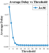
We investigate how the arrival rate λ𝜆\lambda affects the optimal threshold of our policy. In simulations, we set μmm=μp=100subscript𝜇mmsubscript𝜇p100\mu_{\text{mm}}=\mu_{\text{p}}=100, μsub-6=1subscript𝜇sub-61\mu_{\text{sub-6}}=1 and pa=0.6subscript𝑝a0.6p_{\text{a}}=0.6. Then, we investigate how average delay changes as threshold varies given a value of λ{30,35,40,45,50,55}𝜆303540455055\lambda\in\{30,35,40,45,50,55\}. Our simulation results show that for λ=30𝜆30\lambda=30, 353535, 404040, curves of average delay vs different threshold are similar. For lack of space, we only provide results for λ=30𝜆30\lambda=30 here.

Refer to caption
(a) Arrival rate λ=30𝜆30\lambda=30
Refer to caption
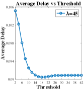
(b) Arrival rate λ=45𝜆45\lambda=45
Refer to caption
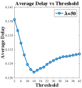
(c) Arrival rate λ=50𝜆50\lambda=50
Refer to caption
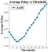
(d) Arrival rate λ=55𝜆55\lambda=55
Figure 5: Average Delay vs Threshold for various arrival rate.

For each result in Fig. 5 (corresponding to a certain λ𝜆\lambda), the optimal threshold corresponds to the lowest average delay. For example, in Fig. 5b (i.e., λ=45𝜆45\lambda=45), the optimal threshold is 18. As shown in Fig. 5a, we can see that if the arrival rate is not high, a small enough threshold provides low delay and as the threshold increases, the delay does not change much. This is because if packets arrive at system slowly, waiting and service times of each packet in mmWave line will be probably less than service time of the sub-6 GHz server. This implies that the mmWave server does not need the aid of the sub-6 GHz server. On the contrary, adding packets to the sub-6 GHz server increases delay because the average service rate of the mmWave is much higher than that of the sub-6 GHz. In addition, Fig. 5b to Fig. 5d demonstrate that the optimal threshold decreases with the arrival rate. This is expected since a faster arrival rate may increase waiting time, which increases the chance of routing through the sub-6 GHz interface.

V-B Benefits from the Sub-6 GHz with Threshold-Type Policy

In this section, we demonstrate benefits of the sub-6 GHz interface to combat the effects of blockage and intermittent connectivity, especially under heavy traffic scenarios. To this end, we compare delay performance in systems with and without the sub-6 GHz. For the system with the sub-6 GHz (our integrated system), the proposed threshold-type policy is utilized. For the system without the sub-6 GHz server, no scheduling policy applies since only mmWave interface exists in the system. To provide a more clear exhibition of our simulation results, we define relative delay improvement W^^𝑊\hat{W} as follows:

W^=W¯(no sub-6)W¯(with sub-6)W¯(no sub-6);^𝑊¯𝑊no sub-6¯𝑊with sub-6¯𝑊no sub-6\displaystyle\hat{W}=\frac{\bar{W}(\text{no sub-6})-\bar{W}(\text{with sub-6})}{\bar{W}(\text{no sub-6})};

where W¯(with sub-6)¯𝑊with sub-6\bar{W}(\text{with sub-6}) and W¯(no sub-6)¯𝑊no sub-6\bar{W}(\text{no sub-6}) denote the average delay in the integrated system and that in the system without the sub-6 GHz server, respectively.
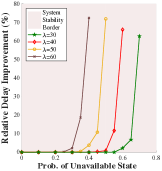
Refer to caption
(a) X-Z view
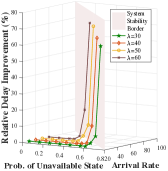
Refer to caption
(b) 3D view
Figure 6: Delay Performance vs Probability of Unavailable State.

In simulation, we investigate how W^^𝑊\hat{W} changes as probability of unavailable state (i.e., pnasubscript𝑝nap_{\text{na}}) increases from 00 to the largest value that ensures stability of the system under fixed arrival rate. We repeat the simulation for different arrival rates. From the results shown in Fig. 6a, we observe that for a certain arrival rate, benefits of the sub-6 GHz interface becomes more pronounced as the probability of unavailable state increases. For instance, for the arrival rate of λ=60𝜆60\lambda=60, there is up to 70%percent7070\% delay reduction using the integrated architecture paired with the threshold-based policy. Furthermore, in order to exhibit the excellent delay performance in heavy traffic scenarios, in Fig. 6 we introduce a system stability border which is a three dimensional plate that is expressed as λ=μsub-6+(1pna)μmm𝜆subscript𝜇sub-61subscript𝑝nasubscript𝜇mm\lambda=\mu_{\text{sub-6}}+(1-p_{\text{na}})\mu_{\text{mm}}. As shown in Fig. 6b, the sub-6 GHz interface becomes more beneficial as either the arrival rate or probability of unavailable state increases, i.e., heavy traffic scenarios.

V-C Comparison with MaxWeight Policy

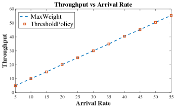
In this section, we investigate the performance of the threshold-type policy compared with the MaxWeight policy. From Fig. 5, we concluded that the optimal threshold is related to the arrival rate. Hence, for each value of λ𝜆\lambda, we use the corresponding optimal threshold. From Fig. 7, we note that the threshold-type policy achieves a better delay performance compared with the MaxWeight policy, while it provides a similar throughput performance. We note that the advantage of our threshold-type policy in delay performance over MaxWeight gets smaller when the arrival rate increases.
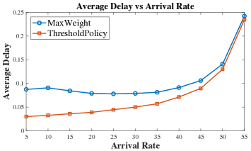
Refer to caption
(a) Delay Performance
Refer to caption
(b) Throughput Performance
Figure 7: Delay and throughput performance of our proposed threshold-type policy compared with MaxWeight policy.

VI Conclusion

In this paper, we considered an integrated sub-6 GHz – mmWave architecture wherein the sub-6 GHz is used as a fallback mechanism to combat blockage and intermittent nature of the mmWave communication. In this case, the arrival packets can be transmitted using the mmWave or sub-6 GHz interface or both. We investigated the optimal packet scheduling policy such that the expected total discounted delay and the average delay are minimized and showed that the optimal policy is of the threshold-type. Through numerical results, we further investigated the delay and throughput performance of our policy to demonstrate that the threshold-type policy in fact provides a much smaller delay compared with the MaxWeight policy, while it achieves a similar throughput performance.

Appendix A Proof of Theorem 1

Note that zero function (i.e., v=0𝑣0v=0) satisfies all properties in Theorem 1. Besides, it is known that for any function fV𝑓𝑉f\in V, limn(n)f=Jβsubscript𝑛superscript𝑛𝑓subscript𝐽𝛽\lim_{n\rightarrow\infty}\mathcal{L}^{(n)}f=J_{\beta}. Thus, in order to show that Jβsubscript𝐽𝛽J_{\beta} satisfies all properties in Theorem 1, we start with zero function and show that v𝑣\mathcal{L}v satisfies the properties if v𝑣v satisfies the properties in Theorem 1. For sake of exposition of the following proof, define K𝐬subscript𝐾𝐬K_{\mathbf{s}} as the set of admissible actions in state 𝐬Q𝐬𝑄\mathbf{s}\in Q.

Property (a): By the definition of operator \mathcal{L} (Eq. (11)), we show the result by respectively proving following inequalities:

(1)minu0v(u0(𝒜0(A1(𝐪))))minu0v(u0(𝒜0(Ah(𝐪))))(1)subscriptsubscript𝑢0𝑣subscript𝑢0subscript𝒜0subscript𝐴1𝐪subscriptsubscript𝑢0𝑣subscript𝑢0subscript𝒜0subscript𝐴𝐪\displaystyle\text{(1)}\ \min\limits_{u_{0}}v\big{(}u_{0}\left(\mathcal{A}_{0}\left(A_{1}\left(\mathbf{q}\right)\right)\right)\big{)}\leq\min\limits_{u_{0}}v\big{(}u_{0}\left(\mathcal{A}_{0}\left(A_{h}\left(\mathbf{q}\right)\right)\right)\big{)}
(2)minu1v(u1(𝒯(A1(𝐪))))minu1v(u1(𝒯(Ah(𝐪))))(2)subscriptsubscript𝑢1𝑣subscript𝑢1𝒯subscript𝐴1𝐪subscriptsubscript𝑢1𝑣subscript𝑢1𝒯subscript𝐴𝐪\displaystyle\text{(2)}\ \min\limits_{u_{1}}v\big{(}u_{1}\left(\mathcal{T}\left(A_{1}\left(\mathbf{q}\right)\right)\right)\big{)}\leq\min\limits_{u_{1}}v\big{(}u_{1}\left(\mathcal{T}\left(A_{h}\left(\mathbf{q}\right)\right)\right)\big{)}
(3)minu2v(u2(𝒟1(A1(𝐪))))minu2v(u2(𝒟1(Ah(𝐪))))(3)subscriptsubscript𝑢2𝑣subscript𝑢2subscript𝒟1subscript𝐴1𝐪subscriptsubscript𝑢2𝑣subscript𝑢2subscript𝒟1subscript𝐴𝐪\displaystyle\text{(3)}\ \min\limits_{u_{2}}v\big{(}u_{2}\left(\mathcal{D}_{1}\left(A_{1}\left(\mathbf{q}\right)\right)\right)\big{)}\leq\min\limits_{u_{2}}v\big{(}u_{2}\left(\mathcal{D}_{1}\left(A_{h}\left(\mathbf{q}\right)\right)\right)\big{)}
(4)minu3v(u3(𝒟2(A1(𝐪))))minu3v(u3(𝒟2(Ah(𝐪)))).(4)subscriptsubscript𝑢3𝑣subscript𝑢3subscript𝒟2subscript𝐴1𝐪subscriptsubscript𝑢3𝑣subscript𝑢3subscript𝒟2subscript𝐴𝐪\displaystyle\text{(4)}\ \min\limits_{u_{3}}v\big{(}u_{3}\left(\mathcal{D}_{2}\left(A_{1}\left(\mathbf{q}\right)\right)\right)\big{)}\leq\min\limits_{u_{3}}v\big{(}u_{3}\left(\mathcal{D}_{2}\left(A_{h}\left(\mathbf{q}\right)\right)\right)\big{)}.

(1): Use 𝐬1subscript𝐬1\mathbf{s}_{1} and 𝐬2subscript𝐬2\mathbf{s}_{2} to denote 𝒜0(A1(𝐪))=(q0,1,q1,l2)subscript𝒜0subscript𝐴1𝐪subscript𝑞01subscript𝑞1subscript𝑙2\mathcal{A}_{0}\left(A_{1}\left(\mathbf{q}\right)\right)=\left(q_{0},1,q_{1},l_{2}\right) and 𝒜0(Ah(𝐪))=(q0+1,0,q1,l2)subscript𝒜0subscript𝐴𝐪subscript𝑞010subscript𝑞1subscript𝑙2\mathcal{A}_{0}\left(A_{h}\left(\mathbf{q}\right)\right)=\left(q_{0}+1,0,q_{1},l_{2}\right), respectively. Then, in order to show (1), we only need to show that for each a2K𝐬2subscript𝑎2subscript𝐾subscript𝐬2a_{2}\in K_{\mathbf{s}_{2}}, there exists a1K𝐬1subscript𝑎1subscript𝐾subscript𝐬1a_{1}\in K_{\mathbf{s}_{1}} such that v(a2(𝐬2))v(a1(𝐬1))𝑣subscript𝑎2subscript𝐬2𝑣subscript𝑎1subscript𝐬1v(a_{2}(\mathbf{s}_{2}))\geq v(a_{1}(\mathbf{s}_{1})). Same logic will also be used in the following proof for other case s.

Generally, {Ah,A1}K𝐬2subscript𝐴subscript𝐴1subscript𝐾subscript𝐬2\{A_{h},A_{1}\}\subseteq K_{\mathbf{s}_{2}} and AhK𝐬1subscript𝐴subscript𝐾subscript𝐬1A_{h}\in K_{\mathbf{s}_{1}}. Then, we have

v(Ah(𝐬2))𝑣subscript𝐴subscript𝐬2\displaystyle v\left(A_{h}\left(\mathbf{s}_{2}\right)\right) (a)v(A1(𝐬2))=v(Ah(𝐬1)).superscript(a)absent𝑣subscript𝐴1subscript𝐬2𝑣subscript𝐴subscript𝐬1\displaystyle\stackrel{{\scriptstyle\text{(a)}}}{{\geq}}v\left(A_{1}\left(\mathbf{s}_{2}\right)\right)=v\left(A_{h}\left(\mathbf{s}_{1}\right)\right).

If l2=0subscript𝑙20l_{2}=0, then A2K𝐬2subscript𝐴2subscript𝐾subscript𝐬2A_{2}\in K_{\mathbf{s}_{2}} and ArK𝐬1subscript𝐴𝑟subscript𝐾subscript𝐬1A_{r}\in K_{\mathbf{s}_{1}}. Notice that Ar(𝐬1)=(q0,0,q1,1)subscript𝐴𝑟subscript𝐬1subscript𝑞00subscript𝑞11A_{r}\left(\mathbf{s}_{1}\right)=\left(q_{0},0,q_{1},1\right) by property (c). In the case, we obtain

v(A2(𝐬2))=v(Ar(𝐬1)).𝑣subscript𝐴2subscript𝐬2𝑣subscript𝐴𝑟subscript𝐬1v\left(A_{2}\left(\mathbf{s}_{2}\right)\right)=v\left(A_{r}\left(\mathbf{s}_{1}\right)\right).

If l2=0subscript𝑙20l_{2}=0 and q11subscript𝑞11q_{1}\geq 1, then ArA𝐬2subscript𝐴𝑟subscript𝐴subscript𝐬2A_{r}\in A_{\mathbf{s}_{2}} and we have

v(Ar(𝐬2))𝑣subscript𝐴𝑟subscript𝐬2\displaystyle v\left(A_{r}\left(\mathbf{s}_{2}\right)\right) (b)v(A2(𝐬2))=v(Ar(𝐬1)).superscript(b)absent𝑣subscript𝐴2subscript𝐬2𝑣subscript𝐴𝑟subscript𝐬1\displaystyle\stackrel{{\scriptstyle\text{(b)}}}{{\geq}}v\left(A_{2}\left(\mathbf{s}_{2}\right)\right)=v\left(A_{r}\left(\mathbf{s}_{1}\right)\right).

(2): Denote 𝒯(A1(𝐪))=(q01,0,q1+1,l2)𝒯subscript𝐴1𝐪subscript𝑞010subscript𝑞11subscript𝑙2\mathcal{T}\left(A_{1}\left(\mathbf{q}\right)\right)=\left(q_{0}-1,0,q_{1}+1,l_{2}\right) as 𝐬3subscript𝐬3\mathbf{s}_{3} and denote 𝒯(Ah(𝐪))=(q0,0,q1,l2)𝒯subscript𝐴𝐪subscript𝑞00subscript𝑞1subscript𝑙2\mathcal{T}\left(A_{h}\left(\mathbf{q}\right)\right)=\left(q_{0},0,q_{1},l_{2}\right) as 𝐬4subscript𝐬4\mathbf{s}_{4}. Generally, AhK𝐬3subscript𝐴subscript𝐾subscript𝐬3A_{h}\in K_{\mathbf{s}_{3}} and {Ah,A1}K𝐬4subscript𝐴subscript𝐴1subscript𝐾subscript𝐬4\{A_{h},A_{1}\}\subseteq K_{\mathbf{s}_{4}}. Thus, we have

v(Ah(𝐬4))𝑣subscript𝐴subscript𝐬4\displaystyle v\left(A_{h}\left(\mathbf{s}_{4}\right)\right) (a)v(A1(𝐬4))superscript(a)absent𝑣subscript𝐴1subscript𝐬4\displaystyle\stackrel{{\scriptstyle\text{(a)}}}{{\geq}}v\left(A_{1}\left(\mathbf{s}_{4}\right)\right)
(c)v(𝒯(q01,1,q1,l2))=v(Ah(𝐬3)).superscript(c)absent𝑣𝒯subscript𝑞011subscript𝑞1subscript𝑙2𝑣subscript𝐴subscript𝐬3\displaystyle\stackrel{{\scriptstyle\text{(c)}}}{{\geq}}v\left(\mathcal{T}\left(q_{0}-1,1,q_{1},l_{2}\right)\right)=v\left(A_{h}\left(\mathbf{s}_{3}\right)\right).

If l2=0subscript𝑙20l_{2}=0, then A2K𝐬4subscript𝐴2subscript𝐾subscript𝐬4A_{2}\in K_{\mathbf{s}_{4}} and ArK𝐬3subscript𝐴𝑟subscript𝐾subscript𝐬3A_{r}\in K_{\mathbf{s}_{3}}. Then, we obtain

v(A2(𝐬4))=v(Ar(𝐬3)).𝑣subscript𝐴2subscript𝐬4𝑣subscript𝐴𝑟subscript𝐬3v\left(A_{2}\left(\mathbf{s}_{4}\right)\right)=v\left(A_{r}\left(\mathbf{s}_{3}\right)\right).

If l2=0subscript𝑙20l_{2}=0 and q11subscript𝑞11q_{1}\geq 1, then ArK𝐬4subscript𝐴𝑟subscript𝐾subscript𝐬4A_{r}\in K_{\mathbf{s}_{4}} and we have

v(Ar(𝐬4))𝑣subscript𝐴𝑟subscript𝐬4\displaystyle v(A_{r}(\mathbf{s}_{4})) (b)v(A2(𝐬4))=v(Ar(𝐬3)).superscript(b)absent𝑣subscript𝐴2subscript𝐬4𝑣subscript𝐴𝑟subscript𝐬3\displaystyle\stackrel{{\scriptstyle\text{(b)}}}{{\geq}}v(A_{2}(\mathbf{s}_{4}))=v(A_{r}(\mathbf{s}_{3})).

(3): Denote 𝒟1(A1(𝐪))=(q01,1,(q11)+,l2)subscript𝒟1subscript𝐴1𝐪subscript𝑞011superscriptsubscript𝑞11subscript𝑙2\mathcal{D}_{1}\left(A_{1}\left(\mathbf{q}\right)\right)=\left(q_{0}-1,1,\left(q_{1}-1\right)^{+},l_{2}\right) as 𝐬5subscript𝐬5\mathbf{s}_{5} and denote 𝒟1(Ah(𝐪))=(q0,0,(q11)+,l2)subscript𝒟1subscript𝐴𝐪subscript𝑞00superscriptsubscript𝑞11subscript𝑙2\mathcal{D}_{1}\left(A_{h}\left(\mathbf{q}\right)\right)=\left(q_{0},0,\left(q_{1}-1\right)^{+},l_{2}\right) as 𝐬6subscript𝐬6\mathbf{s}_{6}. Generally, {Ah,A1}K𝐬6subscript𝐴subscript𝐴1subscript𝐾subscript𝐬6\{A_{h},A_{1}\}\subseteq K_{\mathbf{s}_{6}} and AhK𝐬5subscript𝐴subscript𝐾subscript𝐬5A_{h}\in K_{\mathbf{s}_{5}}. Then, we get

v(Ah(𝐬6))𝑣subscript𝐴subscript𝐬6\displaystyle v\left(A_{h}\left(\mathbf{s}_{6}\right)\right) (a)v(A1(𝐬6))=v(Ah(𝐬5)).superscript(a)absent𝑣subscript𝐴1subscript𝐬6𝑣subscript𝐴subscript𝐬5\displaystyle\stackrel{{\scriptstyle\text{(a)}}}{{\geq}}v\left(A_{1}\left(\mathbf{s}_{6}\right)\right)=v\left(A_{h}\left(\mathbf{s}_{5}\right)\right).

If l2=0subscript𝑙20l_{2}=0, then A2K𝐬6subscript𝐴2subscript𝐾subscript𝐬6A_{2}\in K_{\mathbf{s}_{6}} and ArK𝐬5subscript𝐴𝑟subscript𝐾subscript𝐬5A_{r}\in K_{\mathbf{s}_{5}}. Then, we have

v(A2(𝐬6))=v(Ar(𝐬5)).𝑣subscript𝐴2subscript𝐬6𝑣subscript𝐴𝑟subscript𝐬5v\left(A_{2}\left(\mathbf{s}_{6}\right)\right)=v\left(A_{r}\left(\mathbf{s}_{5}\right)\right).

If l2=0subscript𝑙20l_{2}=0 and (q11)+1superscriptsubscript𝑞111\left(q_{1}-1\right)^{+}\geq 1, then ArK𝐬6subscript𝐴𝑟subscript𝐾subscript𝐬6A_{r}\in K_{\mathbf{s}_{6}}. Thus, we get

v(Ar(𝐬6))𝑣subscript𝐴𝑟subscript𝐬6\displaystyle v\left(A_{r}\left(\mathbf{s}_{6}\right)\right) (b)v(A2(𝐬6))=v(Ar(𝐬5)).superscript(b)absent𝑣subscript𝐴2subscript𝐬6𝑣subscript𝐴𝑟subscript𝐬5\displaystyle\stackrel{{\scriptstyle\text{(b)}}}{{\geq}}v\left(A_{2}\left(\mathbf{s}_{6}\right)\right)=v\left(A_{r}\left(\mathbf{s}_{5}\right)\right).

(4): Denote 𝒟2(A1(𝐪))=(q01,1,q1,0)subscript𝒟2subscript𝐴1𝐪subscript𝑞011subscript𝑞10\mathcal{D}_{2}\left(A_{1}\left(\mathbf{q}\right)\right)=\left(q_{0}-1,1,q_{1},0\right) as 𝐬7subscript𝐬7\mathbf{s}_{7} and denote 𝒟2(Ah(𝐪))=(q0,0,q1,0)subscript𝒟2subscript𝐴𝐪subscript𝑞00subscript𝑞10\mathcal{D}_{2}\left(A_{h}\left(\mathbf{q}\right)\right)=\left(q_{0},0,q_{1},0\right) as 𝐬8subscript𝐬8\mathbf{s}_{8}. Generally, {Ah,A1,A2}K𝐬8subscript𝐴subscript𝐴1subscript𝐴2subscript𝐾subscript𝐬8\{A_{h},A_{1},A_{2}\}\subseteq K_{\mathbf{s}_{8}} and {Ah,Ar}K𝐬7subscript𝐴subscript𝐴𝑟subscript𝐾subscript𝐬7\{A_{h},A_{r}\}\subseteq K_{\mathbf{s}_{7}}. Then, we obtain

v(Ah(𝐬8))(a)v(A1(𝐬8))=v(Ah(𝐬7)),superscript(a)𝑣subscript𝐴subscript𝐬8𝑣subscript𝐴1subscript𝐬8𝑣subscript𝐴subscript𝐬7\displaystyle v\left(A_{h}\left(\mathbf{s}_{8}\right)\right)\stackrel{{\scriptstyle\text{(a)}}}{{\geq}}v\left(A_{1}\left(\mathbf{s}_{8}\right)\right)=v\left(A_{h}\left(\mathbf{s}_{7}\right)\right),
v(A2(𝐬8))=v(Ar(𝐬7)).𝑣subscript𝐴2subscript𝐬8𝑣subscript𝐴𝑟subscript𝐬7\displaystyle v\left(A_{2}\left(\mathbf{s}_{8}\right)\right)=v\left(A_{r}\left(\mathbf{s}_{7}\right)\right).

If q11subscript𝑞11q_{1}\geq 1, ArK𝐬8subscript𝐴𝑟subscript𝐾subscript𝐬8A_{r}\in K_{\mathbf{s}_{8}}, then we have

v(Ar(𝐬8))𝑣subscript𝐴𝑟subscript𝐬8\displaystyle v\left(A_{r}\left(\mathbf{s}_{8}\right)\right) (b)v(A2(𝐬8))=v(Ar(𝐬7)).superscript(b)absent𝑣subscript𝐴2subscript𝐬8𝑣subscript𝐴𝑟subscript𝐬7\displaystyle\stackrel{{\scriptstyle\text{(b)}}}{{\geq}}v\left(A_{2}\left(\mathbf{s}_{8}\right)\right)=v\left(A_{r}\left(\mathbf{s}_{7}\right)\right).

Therefore we conclude that v(A1(𝐪))v(Ah(𝐪))𝑣subscript𝐴1𝐪𝑣subscript𝐴𝐪\mathcal{L}v\left(A_{1}\left(\mathbf{q}\right)\right)\leq\mathcal{L}v\left(A_{h}\left(\mathbf{q}\right)\right).

Property (b): Notice that by property (c), Ar(𝐪)=(q0,0,q1,1)subscript𝐴𝑟𝐪subscript𝑞00subscript𝑞11A_{r}(\mathbf{q})=(q_{0},0,q_{1},1), if l1=1subscript𝑙11l_{1}=1; otherwise, Ar(𝐪)=(q0,0,q11,1)subscript𝐴𝑟𝐪subscript𝑞00subscript𝑞111A_{r}(\mathbf{q})=(q_{0},0,q_{1}-1,1).

As for the case l1=0subscript𝑙10l_{1}=0: the only thing for us to note is that if q1=1subscript𝑞11q_{1}=1, then 𝒟1(A2(𝐪))=(q01,0,0,1)subscript𝒟1subscript𝐴2𝐪subscript𝑞01001\mathcal{D}_{1}\left(A_{2}\left(\mathbf{q}\right)\right)=\left(q_{0}-1,0,0,1\right) and 𝒟1(Ar(𝐪))=(q0,0,0,1)subscript𝒟1subscript𝐴𝑟𝐪subscript𝑞0001\mathcal{D}_{1}\left(A_{r}\left(\mathbf{q}\right)\right)=\left(q_{0},0,0,1\right). Thus, by monotonicity property (e), we directly obtain that minu2v(u2(𝒟1(A2(𝐪))))minu2v(u2(𝒟1(Ar(𝐪))))subscriptsubscript𝑢2𝑣subscript𝑢2subscript𝒟1subscript𝐴2𝐪subscriptsubscript𝑢2𝑣subscript𝑢2subscript𝒟1subscript𝐴𝑟𝐪\min_{u_{2}}{v\left(u_{2}\left(\mathcal{D}_{1}\left(A_{2}\left(\mathbf{q}\right)\right)\right)\right)}\leq\min_{u_{2}}{v\left(u_{2}\left(\mathcal{D}_{1}\left(A_{r}\left(\mathbf{q}\right)\right)\right)\right)}. With this and similar argument in proof of property (a), we can obtain that for q01subscript𝑞01q_{0}\geq 1 and q11subscript𝑞11q_{1}\geq 1, v(A2(q0,0,q1,0))v(Ar(q0,0,q1,0))𝑣subscript𝐴2subscript𝑞00subscript𝑞10𝑣subscript𝐴𝑟subscript𝑞00subscript𝑞10\mathcal{L}v\left(A_{2}\left(q_{0},0,q_{1},0\right)\right)\leq\mathcal{L}v\left(A_{r}\left(q_{0},0,q_{1},0\right)\right).

As for the case l1=1subscript𝑙11l_{1}=1: the case can be proved with similar argument and logic in proof for property (a).

Property (c): The property can be easily shown with similar logic and argument in proof for property (a) and (b).

Property (d): With similar argument, we easily obtain that minu0v(u0(𝒜0(A1(𝐪))))minu0v(u0(𝒜0(A2(𝐪))))subscriptsubscript𝑢0𝑣subscript𝑢0subscript𝒜0subscript𝐴1𝐪subscriptsubscript𝑢0𝑣subscript𝑢0subscript𝒜0subscript𝐴2𝐪\min_{u_{0}}v\left(u_{0}\left(\mathcal{A}_{0}\left(A_{1}\left(\mathbf{q}\right)\right)\right)\right)\leq\min_{u_{0}}v\left(u_{0}\left(\mathcal{A}_{0}\left(A_{2}\left(\mathbf{q}\right)\right)\right)\right), where 𝐪=(q0,0,0,0)𝐪subscript𝑞0000\mathbf{q}=\left(q_{0},0,0,0\right). It remains to show

μpB1+paμmmB2+μsub-6B2subscript𝜇psubscript𝐵1subscript𝑝asubscript𝜇mmsubscript𝐵2subscript𝜇sub-6subscript𝐵2\displaystyle\mu_{\text{p}}B_{1}+p_{\text{a}}\mu_{\text{mm}}B_{2}+\mu_{\text{sub-6}}B_{2}
\displaystyle\leq μpB3+paμmmB3+μsub-6B4.subscript𝜇psubscript𝐵3subscript𝑝asubscript𝜇mmsubscript𝐵3subscript𝜇sub-6subscript𝐵4\displaystyle\mu_{\text{p}}B_{3}+p_{\text{a}}\mu_{\text{mm}}B_{3}+\mu_{\text{sub-6}}B_{4}. (28)

where

B1minu1v(u1(q01,0,1,0))subscript𝐵1subscriptsubscript𝑢1𝑣subscript𝑢1subscript𝑞01010\displaystyle B_{1}\triangleq\min_{u_{1}}v\left(u_{1}\left(q_{0}-1,0,1,0\right)\right)
B2minu2v(u2(q01,1,0,0))=minu3v(u3(q01,1,0,0))subscript𝐵2subscriptsubscript𝑢2𝑣subscript𝑢2subscript𝑞01100subscriptsubscript𝑢3𝑣subscript𝑢3subscript𝑞01100\displaystyle B_{2}\triangleq\min_{u_{2}}v\left(u_{2}\left(q_{0}-1,1,0,0\right)\right)=\min_{u_{3}}v\left(u_{3}\left(q_{0}-1,1,0,0\right)\right)
B3minu1v(u1(q01,0,0,1))=minu2v(u2(q01,0,0,1))subscript𝐵3subscriptsubscript𝑢1𝑣subscript𝑢1subscript𝑞01001subscriptsubscript𝑢2𝑣subscript𝑢2subscript𝑞01001\displaystyle B_{3}\triangleq\min_{u_{1}}v\left(u_{1}\left(q_{0}-1,0,0,1\right)\right)=\min_{u_{2}}v\left(u_{2}\left(q_{0}-1,0,0,1\right)\right)
B4minu3v(u3(q01,0,0,0)).subscript𝐵4subscriptsubscript𝑢3𝑣subscript𝑢3subscript𝑞01000\displaystyle B_{4}\triangleq\min_{u_{3}}v\left(u_{3}\left(q_{0}-1,0,0,0\right)\right).

Note that B4B1B2B3subscript𝐵4subscript𝐵1subscript𝐵2subscript𝐵3B_{4}\leq B_{1}\leq B_{2}\leq B_{3}, which can be shown via similar argument in previous proof.

  1. 1.

    Case that q0>1subscript𝑞01q_{0}>1: notice that by property (a) and (d), B4=v(q02,1,0,0)subscript𝐵4𝑣subscript𝑞02100B_{4}=v\left(q_{0}-2,1,0,0\right) and by property (a), B3=v(q02,1,0,1)subscript𝐵3𝑣subscript𝑞02101B_{3}=v\left(q_{0}-2,1,0,1\right).

    1. (a)

      If v(q01,1,0,0)<v(q02,1,0,1)𝑣subscript𝑞01100𝑣subscript𝑞02101v\left(q_{0}-1,1,0,0\right)<v\left(q_{0}-2,1,0,1\right), then B2=v(q01,1,0,0)<B3subscript𝐵2𝑣subscript𝑞01100subscript𝐵3B_{2}=v(q_{0}-1,1,0,0)<B_{3}. It implies that the sub-6 GHz interface is not preferable in the case. Then, B2B41μsub-6subscript𝐵2subscript𝐵41subscript𝜇sub-6B_{2}-B_{4}\leq\frac{1}{\mu_{\text{sub-6}}} Besides, since the least time that is required for an event to happen is min{1λ,1μp,1paμmm,1μsub-6}1𝜆1subscript𝜇p1subscript𝑝asubscript𝜇mm1subscript𝜇sub-6\min\left\{\frac{1}{\lambda},\frac{1}{\mu_{\text{p}}},\frac{1}{p_{\text{a}}\mu_{\text{mm}}},\frac{1}{\mu_{\text{sub-6}}}\right\}=min{1λ,1μp,1paμmm}1𝜆1subscript𝜇p1subscript𝑝asubscript𝜇mm\min\left\{\frac{1}{\lambda},\frac{1}{\mu_{\text{p}}},\frac{1}{p_{\text{a}}\mu_{\text{mm}}}\right\}, we have B3B2min{1λ,1μp,1paμmm}subscript𝐵3subscript𝐵21𝜆1subscript𝜇p1subscript𝑝asubscript𝜇mmB_{3}-B_{2}\geq\min\left\{\frac{1}{\lambda},\frac{1}{\mu_{\text{p}}},\frac{1}{p_{\text{a}}\mu_{\text{mm}}}\right\}. Therefore, we have

      μp(B1B3)+paμmm(B2B3)+μsub-6(B2B4)subscript𝜇psubscript𝐵1subscript𝐵3subscript𝑝asubscript𝜇mmsubscript𝐵2subscript𝐵3subscript𝜇sub-6subscript𝐵2subscript𝐵4\displaystyle\mu_{\text{p}}\left(B_{1}-B_{3}\right)+p_{\text{a}}\mu_{\text{mm}}\left(B_{2}-B_{3}\right)+\mu_{\text{sub-6}}\left(B_{2}-B_{4}\right)
      \displaystyle\leq (μp+paμmm)(B2B3)+μsub-6(B2B4)subscript𝜇psubscript𝑝asubscript𝜇mmsubscript𝐵2subscript𝐵3subscript𝜇sub-6subscript𝐵2subscript𝐵4\displaystyle\left(\mu_{\text{p}}+p_{\text{a}}\mu_{\text{mm}}\right)\left(B_{2}-B_{3}\right)+\mu_{\text{sub-6}}\left(B_{2}-B_{4}\right)
      \displaystyle\leq μsub-6μsub-6(μp+paμmm)min{1λ,1μp,1paμmm}0.subscript𝜇sub-6subscript𝜇sub-6subscript𝜇psubscript𝑝asubscript𝜇mm1𝜆1subscript𝜇p1subscript𝑝asubscript𝜇mm0\displaystyle\frac{\mu_{\text{sub-6}}}{\mu_{\text{sub-6}}}-\left(\mu_{\text{p}}+p_{\text{a}}\mu_{\text{mm}}\right)\min\left\{\frac{1}{\lambda},\frac{1}{\mu_{\text{p}}},\frac{1}{p_{\text{a}}\mu_{\text{mm}}}\right\}\leq 0.
    2. (b)

      If v(q01,1,0,0)v(q02,1,0,1)𝑣subscript𝑞01100𝑣subscript𝑞02101v\left(q_{0}-1,1,0,0\right)\geq v\left(q_{0}-2,1,0,1\right), which implies the sub-6 GHz interface should be utilized in the case, then B2=B3=v(q02,1,0,1)subscript𝐵2subscript𝐵3𝑣subscript𝑞02101B_{2}=B_{3}=v\left(q_{0}-2,1,0,1\right) and B1=v(q02,0,1,1)subscript𝐵1𝑣subscript𝑞02011B_{1}=v\left(q_{0}-2,0,1,1\right). For the best case, the smallest difference between B2subscript𝐵2B_{2} and B1subscript𝐵1B_{1} is 1μp1subscript𝜇p\frac{1}{\mu_{\text{p}}}. Besides, B3B41μsub-6subscript𝐵3subscript𝐵41subscript𝜇sub-6B_{3}-B_{4}\leq\frac{1}{\mu_{\text{sub-6}}}. Thus, inequality (28) holds.

  2. 2.

    Case that q0=1subscript𝑞01q_{0}=1: we have B2B41μp+1paμmmsubscript𝐵2subscript𝐵41subscript𝜇p1subscript𝑝asubscript𝜇mmB_{2}-B_{4}\leq\frac{1}{\mu_{\text{p}}}+\frac{1}{p_{\text{a}}\mu_{\text{mm}}} and B3B2min{1λ,1μp,1paμmm}subscript𝐵3subscript𝐵21𝜆1subscript𝜇p1subscript𝑝asubscript𝜇mmB_{3}-B_{2}\geq\min\left\{\frac{1}{\lambda},\frac{1}{\mu_{\text{p}}},\frac{1}{p_{\text{a}}\mu_{\text{mm}}}\right\}. Then, the remaining proof is the same as that in (1) for case q0>1subscript𝑞01q_{0}>1.

Property (e): Now we check monotonicity:

v(q0+1,l1,q1,l2)𝑣subscript𝑞01subscript𝑙1subscript𝑞1subscript𝑙2\displaystyle\mathcal{L}v\left(q_{0}+1,l_{1},q_{1},l_{2}\right)
=\displaystyle= (q0+l1+q1+l2+1)subscript𝑞0subscript𝑙1subscript𝑞1subscript𝑙21\displaystyle\left(q_{0}+l_{1}+q_{1}+l_{2}+1\right)
+βmin𝐮{λv(u0(𝒜0(q0+1,l1,q1,l2)))\displaystyle+\beta\min_{\mathbf{u}}\big{\{}\lambda v\left(u_{0}\left(\mathcal{A}_{0}\left(q_{0}+1,l_{1},q_{1},l_{2}\right)\right)\right)
+μpv(u1(𝒯(q0+1,l1,q1,l2)))subscript𝜇p𝑣subscript𝑢1𝒯subscript𝑞01subscript𝑙1subscript𝑞1subscript𝑙2\displaystyle+\mu_{\text{p}}v\left(u_{1}\left(\mathcal{T}\left(q_{0}+1,l_{1},q_{1},l_{2}\right)\right)\right)
+paμmmv(u2(𝒟1(q0+1,l1,q1,l2)))subscript𝑝asubscript𝜇mm𝑣subscript𝑢2subscript𝒟1subscript𝑞01subscript𝑙1subscript𝑞1subscript𝑙2\displaystyle+p_{\text{a}}\mu_{\text{mm}}v\left(u_{2}\left(\mathcal{D}_{1}\left(q_{0}+1,l_{1},q_{1},l_{2}\right)\right)\right)
+μsub-6v(u3(𝒟2(q0+1,l1,q1,l2)))}\displaystyle+\mu_{\text{sub-6}}v\left(u_{3}\left(\mathcal{D}_{2}\left(q_{0}+1,l_{1},q_{1},l_{2}\right)\right)\right)\big{\}}
(e)superscript(e)\displaystyle\stackrel{{\scriptstyle\text{(e)}}}{{\geq}} (q0+l1+q1+l2)+βmin𝐮{λv(u0(𝒜0(q0,l1,q1,l2)))\displaystyle\left(q_{0}+l_{1}+q_{1}+l_{2}\right)+\beta\min_{\mathbf{u}}\big{\{}\lambda v\left(u_{0}\left(\mathcal{A}_{0}\left(q_{0},l_{1},q_{1},l_{2}\right)\right)\right)
+μpv(u1(𝒯(q0,l1,q1,l2)))subscript𝜇p𝑣subscript𝑢1𝒯subscript𝑞0subscript𝑙1subscript𝑞1subscript𝑙2\displaystyle+\mu_{\text{p}}v\left(u_{1}\left(\mathcal{T}\left(q_{0},l_{1},q_{1},l_{2}\right)\right)\right)
+paμmmv(u2(𝒟1(q0,l1,q1,l2)))subscript𝑝asubscript𝜇mm𝑣subscript𝑢2subscript𝒟1subscript𝑞0subscript𝑙1subscript𝑞1subscript𝑙2\displaystyle+p_{\text{a}}\mu_{\text{mm}}v\left(u_{2}\left(\mathcal{D}_{1}\left(q_{0},l_{1},q_{1},l_{2}\right)\right)\right)
+μsub-6v(u3(𝒟2(q0,l1,q1,l2)))}\displaystyle+\mu_{\text{sub-6}}v\left(u_{3}\left(\mathcal{D}_{2}\left(q_{0},l_{1},q_{1},l_{2}\right)\right)\right)\big{\}}
=\displaystyle= v(q0,l1,q1,l2).𝑣subscript𝑞0subscript𝑙1subscript𝑞1subscript𝑙2\displaystyle\mathcal{L}v\left(q_{0},l_{1},q_{1},l_{2}\right).

Similarly, we can obtain that v(q0,l1,q1+1,l2)v(q0,l1,q1,l2)𝑣subscript𝑞0subscript𝑙1subscript𝑞11subscript𝑙2𝑣subscript𝑞0subscript𝑙1subscript𝑞1subscript𝑙2\mathcal{L}v\left(q_{0},l_{1},q_{1}+1,l_{2}\right)\geq\mathcal{L}v\left(q_{0},l_{1},q_{1},l_{2}\right), v(q0,1,q1,l2)v(q0,0,q1,l2)𝑣subscript𝑞01subscript𝑞1subscript𝑙2𝑣subscript𝑞00subscript𝑞1subscript𝑙2\mathcal{L}v\left(q_{0},1,q_{1},l_{2}\right)\geq\mathcal{L}v\left(q_{0},0,q_{1},l_{2}\right) and v(q0,l1,q1,1)v(q0,l1,q1,0)𝑣subscript𝑞0subscript𝑙1subscript𝑞11𝑣subscript𝑞0subscript𝑙1subscript𝑞10\mathcal{L}v\left(q_{0},l_{1},q_{1},1\right)\geq\mathcal{L}v\left(q_{0},l_{1},q_{1},0\right).

Appendix B Proof of Lemma 1

Note that Jβ0(x,q1,l2)=x+q1+l2subscriptsuperscript𝐽0𝛽𝑥subscript𝑞1subscript𝑙2𝑥subscript𝑞1subscript𝑙2J^{0}_{\beta}\left(x,q_{1},l_{2}\right)=x+q_{1}+l_{2} and Jβ0subscriptsuperscript𝐽0𝛽J^{0}_{\beta}\in\mathcal{F} obviously. By Eq. (16), it remains to show that Tβnsubscriptsuperscript𝑇𝑛𝛽T^{n}_{\beta}\in\mathcal{F} and then Jβn+1subscriptsuperscript𝐽𝑛1𝛽J^{n+1}_{\beta}\in\mathcal{F} given Jβnsubscriptsuperscript𝐽𝑛𝛽J^{n}_{\beta}\in\mathcal{F}. Before our proof, we provide some properties extended from Definition 2, which will be used in the following proof.

Extended properties from Definition 2:

2f(x,q1,1)f(x+1,q1,1)+f(x1,q1,1)2𝑓𝑥subscript𝑞11𝑓𝑥1subscript𝑞11𝑓𝑥1subscript𝑞11\displaystyle 2f\left(x,q_{1},1\right)\leq f\left(x+1,q_{1},1\right)+f\left(x-1,q_{1},1\right) (29)
2f(0,q1,1)f(1,q1,1)+f(0,q11,1)2𝑓0subscript𝑞11𝑓1subscript𝑞11𝑓0subscript𝑞111\displaystyle 2f\left(0,q_{1},1\right)\leq f\left(1,q_{1},1\right)+f\left(0,q_{1}-1,1\right) (30)
2f(0,q1,1)f(0,q1+1,1)+f(0,q11,1)2𝑓0subscript𝑞11𝑓0subscript𝑞111𝑓0subscript𝑞111\displaystyle 2f\left(0,q_{1},1\right)\leq f\left(0,q_{1}+1,1\right)+f\left(0,q_{1}-1,1\right) (31)
2f(x+1,q1,0)f(x+2,q1,0)+f(x,q1,0)2𝑓𝑥1subscript𝑞10𝑓𝑥2subscript𝑞10𝑓𝑥subscript𝑞10\displaystyle 2f\left(x+1,q_{1},0\right)\leq f\left(x+2,q_{1},0\right)+f\left(x,q_{1},0\right) (32)
2f(0,q1+1,0)f(0,q1,0)+f(0,q1+2,0)2𝑓0subscript𝑞110𝑓0subscript𝑞10𝑓0subscript𝑞120\displaystyle 2f\left(0,q_{1}+1,0\right)\leq f\left(0,q_{1},0\right)+f\left(0,q_{1}+2,0\right) (33)
f(x,q1,1)+f(x1,q1+1,1)𝑓𝑥subscript𝑞11𝑓𝑥1subscript𝑞111\displaystyle f\left(x,q_{1},1\right)+f\left(x-1,q_{1}+1,1\right)
f(x,q1+1,1)+f(x1,q1,1)absent𝑓𝑥subscript𝑞111𝑓𝑥1subscript𝑞11\displaystyle\ \ \ \ \ \ \ \ \ \ \ \ \ \ \leq f\left(x,q_{1}+1,1\right)+f\left(x-1,q_{1},1\right) (34)
f(0,q1+1,0)+f(0,q1+1,1)𝑓0subscript𝑞110𝑓0subscript𝑞111\displaystyle f\left(0,q_{1}+1,0\right)+f\left(0,q_{1}+1,1\right)
f(0,q1,1)+f(1,q1+1,0)absent𝑓0subscript𝑞11𝑓1subscript𝑞110\displaystyle\ \ \ \ \ \ \ \ \ \ \ \ \ \ \leq f\left(0,q_{1},1\right)+f\left(1,q_{1}+1,0\right) (35)
f(x+1,q1,0)+f(x,q1+1,0)𝑓𝑥1subscript𝑞10𝑓𝑥subscript𝑞110\displaystyle f\left(x+1,q_{1},0\right)+f\left(x,q_{1}+1,0\right)
f(x+1,q1+1,0)+f(x,q1,0)absent𝑓𝑥1subscript𝑞110𝑓𝑥subscript𝑞10\displaystyle\ \ \ \ \ \ \ \ \ \ \ \ \ \ \leq f\left(x+1,q_{1}+1,0\right)+f\left(x,q_{1},0\right) (36)

These properties can be obtained from combinations of certain equations in Definition 2. For lack of space, we take Eq. (29) for example, it is obtained by adding Eq. (17) with x𝑥x replaced by x1𝑥1x-1 and Eq. (21).

Given Jβnsuperscriptsubscript𝐽𝛽𝑛J_{\beta}^{n}\in\mathcal{F}, we first show that Tβnsubscriptsuperscript𝑇𝑛𝛽T^{n}_{\beta}\in\mathcal{F}.

  1. 1.

    For Eq. (6): If Tβn(x+2,q1,0)=Jβn(x+2,q1,0)subscriptsuperscript𝑇𝑛𝛽𝑥2subscript𝑞10subscriptsuperscript𝐽𝑛𝛽𝑥2subscript𝑞10T^{n}_{\beta}\left(x+2,q_{1},0\right)=J^{n}_{\beta}\left(x+2,q_{1},0\right), then

    Tβn(x+1,q1,0)+limit-fromsubscriptsuperscript𝑇𝑛𝛽𝑥1subscript𝑞10\displaystyle T^{n}_{\beta}\left(x+1,q_{1},0\right)+ Tβn(x+1,q1,1)subscriptsuperscript𝑇𝑛𝛽𝑥1subscript𝑞11\displaystyle T^{n}_{\beta}\left(x+1,q_{1},1\right)
    Def. 1superscriptDef. 1\displaystyle\stackrel{{\scriptstyle\text{Def. \ref{intermediate value}}}}{{\leq}} Jβn(x+1,q1,0)+Jβn(x+1,q1,1)subscriptsuperscript𝐽𝑛𝛽𝑥1subscript𝑞10subscriptsuperscript𝐽𝑛𝛽𝑥1subscript𝑞11\displaystyle J^{n}_{\beta}\left(x+1,q_{1},0\right)+J^{n}_{\beta}\left(x+1,q_{1},1\right)
    (17)superscript(17)\displaystyle\stackrel{{\scriptstyle\text{\eqref{A2_x}}}}{{\leq}} Jβn(x,q1,1)+Jβn(x+2,q1,0).subscriptsuperscript𝐽𝑛𝛽𝑥subscript𝑞11subscriptsuperscript𝐽𝑛𝛽𝑥2subscript𝑞10\displaystyle J^{n}_{\beta}\left(x,q_{1},1\right)+J^{n}_{\beta}\left(x+2,q_{1},0\right).

    If Tβn(x+2,q1,0)=Jβn(x+1,q1,1)subscriptsuperscript𝑇𝑛𝛽𝑥2subscript𝑞10subscriptsuperscript𝐽𝑛𝛽𝑥1subscript𝑞11T^{n}_{\beta}\left(x+2,q_{1},0\right)=J^{n}_{\beta}\left(x+1,q_{1},1\right), then

    Tβn(x+1,q1,0)+limit-fromsubscriptsuperscript𝑇𝑛𝛽𝑥1subscript𝑞10\displaystyle T^{n}_{\beta}\left(x+1,q_{1},0\right)+ Tβn(x+1,q1,1)subscriptsuperscript𝑇𝑛𝛽𝑥1subscript𝑞11\displaystyle T^{n}_{\beta}\left(x+1,q_{1},1\right)
    Def. 1superscriptDef. 1\displaystyle\stackrel{{\scriptstyle\text{Def. \ref{intermediate value}}}}{{\leq}} Jβn(x,q1,1)+Jβn(x+1,q1,1).subscriptsuperscript𝐽𝑛𝛽𝑥subscript𝑞11subscriptsuperscript𝐽𝑛𝛽𝑥1subscript𝑞11\displaystyle J^{n}_{\beta}\left(x,q_{1},1\right)+J^{n}_{\beta}\left(x+1,q_{1},1\right).

    Similarly, we can show that Eq. (18), (19) and (20) hold.

  2. 2.

    For Eq. (10): If Tβn(x,q1,0)=Jβn(x,q1,0)subscriptsuperscript𝑇𝑛𝛽𝑥subscript𝑞10subscriptsuperscript𝐽𝑛𝛽𝑥subscript𝑞10T^{n}_{\beta}\left(x,q_{1},0\right)=J^{n}_{\beta}\left(x,q_{1},0\right), then

    Tβn(x,q1,1)+limit-fromsubscriptsuperscript𝑇𝑛𝛽𝑥subscript𝑞11\displaystyle T^{n}_{\beta}\left(x,q_{1},1\right)+ Tβn(x+1,q1,0)subscriptsuperscript𝑇𝑛𝛽𝑥1subscript𝑞10\displaystyle T^{n}_{\beta}\left(x+1,q_{1},0\right)
    Def. 1superscriptDef. 1\displaystyle\stackrel{{\scriptstyle\text{Def. \ref{intermediate value}}}}{{\leq}} Jβn(x,q1,1)+Jβn(x+1,q1,0)subscriptsuperscript𝐽𝑛𝛽𝑥subscript𝑞11subscriptsuperscript𝐽𝑛𝛽𝑥1subscript𝑞10\displaystyle J^{n}_{\beta}\left(x,q_{1},1\right)+J^{n}_{\beta}\left(x+1,q_{1},0\right)
    (21)superscriptitalic-(21italic-)\displaystyle\stackrel{{\scriptstyle\eqref{supermodular1}}}{{\leq}} Jβn(x,q1,0)+Jβn(x+1,q1,1).subscriptsuperscript𝐽𝑛𝛽𝑥subscript𝑞10subscriptsuperscript𝐽𝑛𝛽𝑥1subscript𝑞11\displaystyle J^{n}_{\beta}\left(x,q_{1},0\right)+J^{n}_{\beta}\left(x+1,q_{1},1\right).

    If x1𝑥1x\geq 1 and Tβn(x,q1,0)=Jβn(x1,q1,1)subscriptsuperscript𝑇𝑛𝛽𝑥subscript𝑞10subscriptsuperscript𝐽𝑛𝛽𝑥1subscript𝑞11T^{n}_{\beta}\left(x,q_{1},0\right)=J^{n}_{\beta}\left(x-1,q_{1},1\right), then

    Tβn(x,q1,1)+Tβn(x+1,q1,0)subscriptsuperscript𝑇𝑛𝛽𝑥subscript𝑞11subscriptsuperscript𝑇𝑛𝛽𝑥1subscript𝑞10\displaystyle T^{n}_{\beta}\left(x,q_{1},1\right)+T^{n}_{\beta}\left(x+1,q_{1},0\right)
    Def. 12Jβn(x,q1,1)(29)Jβn(x1,q1,1)+Jβn(x+1,q1,1).superscriptDef. 1absent2subscriptsuperscript𝐽𝑛𝛽𝑥subscript𝑞11superscriptitalic-(29italic-)subscriptsuperscript𝐽𝑛𝛽𝑥1subscript𝑞11subscriptsuperscript𝐽𝑛𝛽𝑥1subscript𝑞11\displaystyle\stackrel{{\scriptstyle\text{Def. \ref{intermediate value}}}}{{\leq}}2J^{n}_{\beta}\left(x,q_{1},1\right)\stackrel{{\scriptstyle\eqref{extension1}}}{{\leq}}J^{n}_{\beta}\left(x-1,q_{1},1\right)+J^{n}_{\beta}\left(x+1,q_{1},1\right).

    If x=0𝑥0x=0, q11subscript𝑞11q_{1}\geq 1 and Tβn(0,q1,0)=Jβn(0,q11,1)subscriptsuperscript𝑇𝑛𝛽0subscript𝑞10subscriptsuperscript𝐽𝑛𝛽0subscript𝑞111T^{n}_{\beta}\left(0,q_{1},0\right)=J^{n}_{\beta}\left(0,q_{1}-1,1\right), then

    Tβn(0,q1,1)+Tβn(1,q1,0)subscriptsuperscript𝑇𝑛𝛽0subscript𝑞11subscriptsuperscript𝑇𝑛𝛽1subscript𝑞10\displaystyle T^{n}_{\beta}\left(0,q_{1},1\right)+T^{n}_{\beta}\left(1,q_{1},0\right)
    Def. 12Jβn(0,q1,1)(30)Jβn(0,q11,1)+Jβn(1,q1,1).superscriptDef. 1absent2subscriptsuperscript𝐽𝑛𝛽0subscript𝑞11superscript(30)subscriptsuperscript𝐽𝑛𝛽0subscript𝑞111subscriptsuperscript𝐽𝑛𝛽1subscript𝑞11\displaystyle\stackrel{{\scriptstyle\text{Def. \ref{intermediate value}}}}{{\leq}}2J^{n}_{\beta}\left(0,q_{1},1\right)\stackrel{{\scriptstyle\text{\eqref{extension2}}}}{{\leq}}J^{n}_{\beta}\left(0,q_{1}-1,1\right)+J^{n}_{\beta}\left(1,q_{1},1\right).
  3. 3.

    For Eq. (11): If Tβn(x,q1,0)=Jβn(x,q1,0)subscriptsuperscript𝑇𝑛𝛽𝑥subscript𝑞10subscriptsuperscript𝐽𝑛𝛽𝑥subscript𝑞10T^{n}_{\beta}\left(x,q_{1},0\right)=J^{n}_{\beta}\left(x,q_{1},0\right), then

    Tβn(x,q1,1)+limit-fromsubscriptsuperscript𝑇𝑛𝛽𝑥subscript𝑞11\displaystyle T^{n}_{\beta}\left(x,q_{1},1\right)+ Tβn(x,q1+1,0)subscriptsuperscript𝑇𝑛𝛽𝑥subscript𝑞110\displaystyle T^{n}_{\beta}\left(x,q_{1}+1,0\right)
    Def. 1superscriptDef. 1\displaystyle\stackrel{{\scriptstyle\text{Def. \ref{intermediate value}}}}{{\leq}} Jβn(x,q1,1)+Jβn(x,q1+1,0)subscriptsuperscript𝐽𝑛𝛽𝑥subscript𝑞11subscriptsuperscript𝐽𝑛𝛽𝑥subscript𝑞110\displaystyle J^{n}_{\beta}\left(x,q_{1},1\right)+J^{n}_{\beta}\left(x,q_{1}+1,0\right)
    (22)superscript(22)\displaystyle\stackrel{{\scriptstyle\text{\eqref{supermodular2}}}}{{\leq}} Jβn(x,q1,0)+Jβn(x,q1+1,1).subscriptsuperscript𝐽𝑛𝛽𝑥subscript𝑞10subscriptsuperscript𝐽𝑛𝛽𝑥subscript𝑞111\displaystyle J^{n}_{\beta}\left(x,q_{1},0\right)+J^{n}_{\beta}\left(x,q_{1}+1,1\right).

    If x1𝑥1x\geq 1 and Tβn(x,q1,0)=Jβn(x1,q1,1)subscriptsuperscript𝑇𝑛𝛽𝑥subscript𝑞10subscriptsuperscript𝐽𝑛𝛽𝑥1subscript𝑞11T^{n}_{\beta}\left(x,q_{1},0\right)=J^{n}_{\beta}\left(x-1,q_{1},1\right), then

    Tβn(x,q1,1)+limit-fromsubscriptsuperscript𝑇𝑛𝛽𝑥subscript𝑞11\displaystyle T^{n}_{\beta}\left(x,q_{1},1\right)+ Tβn(x,q1+1,0)subscriptsuperscript𝑇𝑛𝛽𝑥subscript𝑞110\displaystyle T^{n}_{\beta}\left(x,q_{1}+1,0\right)
    Def. 1superscriptDef. 1\displaystyle\stackrel{{\scriptstyle\text{Def. \ref{intermediate value}}}}{{\leq}} Jβn(x,q1,1)+Jβn(x1,q1+1,1)subscriptsuperscript𝐽𝑛𝛽𝑥subscript𝑞11subscriptsuperscript𝐽𝑛𝛽𝑥1subscript𝑞111\displaystyle J^{n}_{\beta}\left(x,q_{1},1\right)+J^{n}_{\beta}\left(x-1,q_{1}+1,1\right)
    (34)superscript(34)\displaystyle\stackrel{{\scriptstyle\text{\eqref{extension3}}}}{{\leq}} Jβn(x1,q1,1)+Jβn(x,q1+1,1).subscriptsuperscript𝐽𝑛𝛽𝑥1subscript𝑞11subscriptsuperscript𝐽𝑛𝛽𝑥subscript𝑞111\displaystyle J^{n}_{\beta}\left(x-1,q_{1},1\right)+J^{n}_{\beta}\left(x,q_{1}+1,1\right).

    If x=0𝑥0x=0, q11subscript𝑞11q_{1}\geq 1 and Tβn(0,q1,0)=Jβn(0,q11,1)subscriptsuperscript𝑇𝑛𝛽0subscript𝑞10subscriptsuperscript𝐽𝑛𝛽0subscript𝑞111T^{n}_{\beta}\left(0,q_{1},0\right)=J^{n}_{\beta}\left(0,q_{1}-1,1\right), then

    Tβn(0,q1,1)+Tβn(0,q1+1,0)subscriptsuperscript𝑇𝑛𝛽0subscript𝑞11subscriptsuperscript𝑇𝑛𝛽0subscript𝑞110\displaystyle T^{n}_{\beta}\left(0,q_{1},1\right)+T^{n}_{\beta}\left(0,q_{1}+1,0\right)
    Def. 12Jβn(0,q1,1)(31)Jβn(0,q11,1)+Jβn(0,q1+1,1).superscriptDef. 1absent2subscriptsuperscript𝐽𝑛𝛽0subscript𝑞11superscriptitalic-(31italic-)subscriptsuperscript𝐽𝑛𝛽0subscript𝑞111subscriptsuperscript𝐽𝑛𝛽0subscript𝑞111\displaystyle\stackrel{{\scriptstyle\text{Def. \ref{intermediate value}}}}{{\leq}}2J^{n}_{\beta}\left(0,q_{1},1\right)\stackrel{{\scriptstyle\eqref{extension4}}}{{\leq}}J^{n}_{\beta}\left(0,q_{1}-1,1\right)+J^{n}_{\beta}\left(0,q_{1}+1,1\right).
  4. 4.

    For Eq. (12): If Tβn(x+1,q1,l2)=Jβn(x+1,q1,l2)subscriptsuperscript𝑇𝑛𝛽𝑥1subscript𝑞1subscript𝑙2subscriptsuperscript𝐽𝑛𝛽𝑥1subscript𝑞1subscript𝑙2T^{n}_{\beta}\left(x+1,q_{1},l_{2}\right)=J^{n}_{\beta}\left(x+1,q_{1},l_{2}\right), then

    Tβn(x,q1,l2)Def. 1Jβn(x,q1,l2)(23)Jβn(x+1,q1,l2).superscriptDef. 1subscriptsuperscript𝑇𝑛𝛽𝑥subscript𝑞1subscript𝑙2subscriptsuperscript𝐽𝑛𝛽𝑥subscript𝑞1subscript𝑙2superscriptitalic-(23italic-)subscriptsuperscript𝐽𝑛𝛽𝑥1subscript𝑞1subscript𝑙2\displaystyle T^{n}_{\beta}\left(x,q_{1},l_{2}\right)\stackrel{{\scriptstyle\text{Def. \ref{intermediate value}}}}{{\leq}}J^{n}_{\beta}\left(x,q_{1},l_{2}\right)\stackrel{{\scriptstyle\eqref{mono1}}}{{\leq}}J^{n}_{\beta}\left(x+1,q_{1},l_{2}\right).

    If l2=0subscript𝑙20l_{2}=0 and Tβn(x+1,q1,0)=Jβn(x,q1,1)subscriptsuperscript𝑇𝑛𝛽𝑥1subscript𝑞10subscriptsuperscript𝐽𝑛𝛽𝑥subscript𝑞11T^{n}_{\beta}\left(x+1,q_{1},0\right)=J^{n}_{\beta}\left(x,q_{1},1\right), then

    Tβn(x,q1,0)Def. 1Jβn(x,q1,0)(25)Jβn(x,q1,1).superscriptDef. 1subscriptsuperscript𝑇𝑛𝛽𝑥subscript𝑞10subscriptsuperscript𝐽𝑛𝛽𝑥subscript𝑞10superscriptitalic-(25italic-)subscriptsuperscript𝐽𝑛𝛽𝑥subscript𝑞11\displaystyle T^{n}_{\beta}\left(x,q_{1},0\right)\stackrel{{\scriptstyle\text{Def. \ref{intermediate value}}}}{{\leq}}J^{n}_{\beta}\left(x,q_{1},0\right)\stackrel{{\scriptstyle\eqref{mono3}}}{{\leq}}J^{n}_{\beta}\left(x,q_{1},1\right).

    Similarly, we obtain Eq. (24) and Eq. (25).

Next, we show that Jβn+1subscriptsuperscript𝐽𝑛1𝛽J^{n+1}_{\beta}\in\mathcal{F}. According to Eq. (16), we show four terms, say λ𝜆\lambda, μpsubscript𝜇p\mu_{\text{p}}, μmmsubscript𝜇mm\mu_{\text{mm}} and μsub-6subscript𝜇sub-6\mu_{\text{sub-6}} terms, satisfy properties in Definition 2, respectively.

  1. 1.

    For Eq. (6): the difficulty falls in the μpsubscript𝜇p\mu_{\text{p}} and μsub-6subscript𝜇sub-6\mu_{\text{sub-6}} terms. For the μpsubscript𝜇p\mu_{\text{p}} term, the difficulty falls in the case with x=0𝑥0x=0, which can be proved with Eq. (35). For the μsub-6subscript𝜇sub-6\mu_{\text{sub-6}} term, Eq. (17) reduces to Eq. (32).

  2. 2.

    For Eq. (7): the λ𝜆\lambda term obviously holds. As for the μpsubscript𝜇p\mu_{\text{p}} term, the difficulty falls in the case with x=0𝑥0x=0. Actually, it reduces to Eq. (19). As for the μmmsubscript𝜇mm\mu_{\text{mm}} term, the difficulty falls in the case with q1=0subscript𝑞10q_{1}=0. In the case, Eq. (18) reduces to equality. As for μsub-6subscript𝜇sub-6\mu_{\text{sub-6}} term, Eq. (18) reduces to Eq. (36).

  3. 3.

    For Eq. (8): the λ𝜆\lambda and μpsubscript𝜇p\mu_{\text{p}} terms obviously hold. As for the μmmsubscript𝜇mm\mu_{\text{mm}} term, the difficulty falls in the case with q1=0subscript𝑞10q_{1}=0, where Tβn(0,0,0)Tβn(0,1,0)subscriptsuperscript𝑇𝑛𝛽000subscriptsuperscript𝑇𝑛𝛽010T^{n}_{\beta}(0,0,0)\leq T^{n}_{\beta}(0,1,0). In fact, the inequality holds by Eq. (24). As for the μsub-6subscript𝜇sub-6\mu_{\text{sub-6}} term, Eq. (19) reduces to Eq. (33).

  4. 4.

    For Eq. (9): the λ𝜆\lambda, μpsubscript𝜇p\mu_{\text{p}} with x1𝑥1x\geq 1, μmmsubscript𝜇mm\mu_{\text{mm}} with q11subscript𝑞11q_{1}\geq 1 and μsub-6subscript𝜇sub-6\mu_{\text{sub-6}} terms hold obviously. As for the μpsubscript𝜇p\mu_{\text{p}} with x=0𝑥0x=0 term, Eq. (20) reduces to an equation. As for the μmmsubscript𝜇mm\mu_{\text{mm}} with q1=0subscript𝑞10q_{1}=0 term, Eq. (20) reduces to Eq. (23) with q1=0subscript𝑞10q_{1}=0.

  5. 5.

    For Eq. (10): it is obvious that the λ𝜆\lambda, μpsubscript𝜇p\mu_{\text{p}} with x1𝑥1x\geq 1, and μmmsubscript𝜇mm\mu_{\text{mm}} terms hold. Notice that as for the μsub-6subscript𝜇sub-6\mu_{\text{sub-6}} term, Eq. (21) reduces to an equality. As for the μpsubscript𝜇p\mu_{\text{p}} term with x=0𝑥0x=0, Eq. (21) reduces to Eq. (22).

  6. 6.

    For Eq. (11): the difficulty falls in the μsub-6subscript𝜇sub-6\mu_{\text{sub-6}} and μmmsubscript𝜇mm\mu_{\text{mm}} with q1=0subscript𝑞10q_{1}=0 terms. For both of the cases, Eq. (22) reduces to an equality.

  7. 7.

    For Eq. (12): the only difficulty falls in the μpsubscript𝜇p\mu_{\text{p}} term with x=0𝑥0x=0, in which case, Eq. (23) reduces to Eq. (24) with x=0𝑥0x=0.

  8. 8.

    For Eq. (13): the only difficulty falls in the μmmsubscript𝜇mm\mu_{\text{mm}} term with q1=0subscript𝑞10q_{1}=0. In the case, Eq. (24) reduces to an equality.

  9. 9.

    For Eq. (14): the only difficulty falls in the μsub-6subscript𝜇sub-6\mu_{\text{sub-6}} term. Actually, in the case, Eq. (25) reduces to an equality.

Appendix C Proof of Lemma 2

According to Lemma 1, for each n𝑛n\in\mathbb{N}, Jβnsubscriptsuperscript𝐽𝑛𝛽J^{n}_{\beta} satisfies properties (17), (18), (19) and (35). It implies that for either the case x>0𝑥0x>0 or x=0𝑥0x=0, Jβn(x+1,q1,0)Jβn(x,q1,1)subscriptsuperscript𝐽𝑛𝛽𝑥1subscript𝑞10subscriptsuperscript𝐽𝑛𝛽𝑥subscript𝑞11J^{n}_{\beta}\left(x+1,q_{1},0\right)-J^{n}_{\beta}\left(x,q_{1},1\right) or Jβn(0,q1+1,0)Jβn(0,q1,1)subscriptsuperscript𝐽𝑛𝛽0subscript𝑞110subscriptsuperscript𝐽𝑛𝛽0subscript𝑞11J^{n}_{\beta}\left(0,q_{1}+1,0\right)-J^{n}_{\beta}\left(0,q_{1},1\right) increases as x+q1𝑥subscript𝑞1x+q_{1} increases (due to increase of x𝑥x or q1subscript𝑞1q_{1} or both). In other words, the difference between costs resulted from not-adding-to-sub-6 and adding-to-sub-6 increases as the number of packets in FastLane increases. It is known that Jβn(0,1,0)Jβn(1,0,0)Jβn(0,0,1)subscriptsuperscript𝐽𝑛𝛽010subscriptsuperscript𝐽𝑛𝛽100subscriptsuperscript𝐽𝑛𝛽001J^{n}_{\beta}\left(0,1,0\right)\leq J^{n}_{\beta}\left(1,0,0\right)\leq J^{n}_{\beta}\left(0,0,1\right), which means that it’s better to hold the packet in FastLane when there is only one packet in the system. As x+q1𝑥subscript𝑞1x+q_{1} increases, the difference becomes positive, which means that adding-to-sub-6 obtains priority. To sum up, there exists a certain threshold for the queue length of FastLane above which we should add a packet to the sub-6 GHz interface.

References

  • [1] Farooq Khan and Zhouyue Pi. mmWave mobile broadband (MMB): Unleashing the 3–300GHz spectrum. In 34th IEEE Sarnoff Symposium, 2011.
  • [2] Theodore S Rappaport, Shu Sun, Rimma Mayzus, Hang Zhao, Yaniv Azar, Kangping Wang, George N Wong, Jocelyn K Schulz, Mathew Samimi, and Felix Gutierrez. Millimeter wave mobile communications for 5G cellular: It will work! Access, IEEE, 1:335–349, 2013.
  • [3] Sanjib Sur, Ioannis Pefkianakis, Xinyu Zhang, and Kyu-Han Kim. Wifi-assisted 60 ghz wireless networks. In Proceedings of the 23rd Annual International Conference on Mobile Computing and Networking, pages 28–41. ACM, 2017.
  • [4] Yong Niu, Yong Li, Depeng Jin, Li Su, and Dapeng Wu. Blockage robust and efficient scheduling for directional mmwave wpans. IEEE Transactions on Vehicular Technology, 64(2):728–742, 2015.
  • [5] Zulkuf Genc, Umar H Rizvi, Ertan Onur, and Ignas Niemegeers. Robust 60 ghz indoor connectivity: is it possible with reflections? In Vehicular Technology Conference (VTC 2010-Spring), 2010 IEEE 71st, pages 1–5. IEEE, 2010.
  • [6] Sylvain Collonge, Gheorghe Zaharia, and G EL Zein. Influence of the human activity on wide-band characteristics of the 60 ghz indoor radio channel. IEEE Transactions on Wireless Communications, 3(6):2396–2406, 2004.
  • [7] Christopher Slezak, Vasilii Semkin, Sergey Andreev, Yevgeni Koucheryavy, and Sundeep Rangan. Empirical effects of dynamic human-body blockage in 60 ghz communications. arXiv preprint arXiv:1811.06139, 2018.
  • [8] Sanjib Sur, Vignesh Venkateswaran, Xinyu Zhang, and Parmesh Ramanathan. 60 ghz indoor networking through flexible beams: A link-level profiling. In ACM SIGMETRICS Performance Evaluation Review, volume 43, pages 71–84. ACM, 2015.
  • [9] Katsuyoshi Sato and Takeshi Manabe. Estimation of propagation-path visibility for indoor wireless lan systems under shadowing condition by human bodies. In Vehicular Technology Conference, 1998. VTC 98. 48th IEEE, volume 3, pages 2109–2113. IEEE, 1998.
  • [10] Morteza Hashemi, C Emre Koksal, and Ness B Shroff. Out-of-band millimeter wave beamforming and communications to achieve low latency and high energy efficiency in 5G systems. IEEE Transactions on Communications, 66(2):875–888, 2018.
  • [11] Sumit Singh, Federico Ziliotto, Upamanyu Madhow, Elizabeth M Belding, and Mark JW Rodwell. Millimeter wave wpan: Cross-layer modeling and multi-hop architecture. In INFOCOM 2007. 26th IEEE International Conference on Computer Communications. IEEE, pages 2336–2340. IEEE, 2007.
  • [12] Thomas Nitsche, Adriana B Flores, Edward W Knightly, and Joerg Widmer. Steering with eyes closed: mm-wave beam steering without in-band measurement. In Computer Communications (INFOCOM), IEEE Conference on, pages 2416–2424. IEEE, 2015.
  • [13] Anum Ali, NG Prelcic, and RW Heath. Estimating millimeter wave channels using out-of-band measurements. Information Theory and Applications Workshop (ITA), 2016.
  • [14] Morteza Hashemi, Ashutosh Sabharwal, C Emre Koksal, and Ness B Shroff. Efficient beam alignment in millimeter wave systems using contextual bandits. In IEEE INFOCOM 2018-IEEE Conference on Computer Communications, pages 2393–2401. IEEE, 2018.
  • [15] Morteza Hashemi, C Emre Koksal, and Ness B Shroff. Energy-efficient power and bandwidth allocation in an integrated sub-6 GHz–millimeter wave system. arXiv preprint arXiv:1710.00980, 2017.
  • [16] Ronald L. Larsen and Ashok K. Agrawala. Control of a heterogeneous two-server exponential queueing system. IEEE Transactions on Software Engineering, (4):522–526, 1983.
  • [17] Woei Lin and P Kumar. Optimal control of a queueing system with two heterogeneous servers. IEEE Transactions on Automatic control, 29(8):696–703, 1984.
  • [18] P WALRAND. A note on’optimal control of a queueing system with two heterogeneous serves. Systems and Control Letters, 4:131–134, 1984.
  • [19] Ger Koole. A simple proof of the optimality of a threshold policy in a two-server queueing system. Systems & Control Letters, 26(5):301–303, 1995.
  • [20] VV Rykov. Monotone control of queueing systems with heterogeneous servers. Queueing systems, 37(4):391–403, 2001.
  • [21] Ioannis Viniotis and Anthony Ephremides. Extension of the optimality of the threshold policy in heterogeneous multiserver queueing systems. IEEE Transactions on Automatic Control, 33(1):104–109, 1988.
  • [22] Erhun Özkan and Jeffrey P Kharoufeh. Optimal control of a two-server queueing system with failures. Probability in the Engineering and Informational Sciences, 28(4):489–527, 2014.
  • [23] Leandros Tassiulas and Anthony Ephremides. Stability properties of constrained queueing systems and scheduling policies for maximum throughput in multihop radio networks. IEEE transactions on automatic control, 37(12):1936–1948, 1992.
  • [24] Martin L Puterman. Markov decision processes: discrete stochastic dynamic programming. John Wiley & Sons, 2014.
  • [25] Steven A Lippman. Semi-markov decision processes with unbounded rewards. Management Science, 19(7):717–731, 1973.