Scalar Field Dark Matter Spectator During Inflation: The Effect of Self-interaction

Abstract

Nowadays cosmological inflation is the most accepted mechanism to explain the primordial seeds that led to the structure formation observed in the Universe. Current observations are in well agreement to initial adiabatic conditions, which imply that single-scalar-field inflation may be enough to describe the early Universe. However, there are several scenarios where the existence of more than a single field could be relevant during this period, for instance, the situation where the so-called spectator is present. Within the spectator scenario we can find the possibility that an ultra-light scalar field dark matter candidate could coexist with the inflaton. In this work we study this possibility where the additional scalar field could be free or self-interacting. We use isocurvature observations to constrain the free parameters of the model.

Inflation – Isocurvature – Scalar field – Dark Matter

I Introduction

It is well accepted that the primordial seeds of the structure formation in the Universe were generated by quantum fluctuations given a scalar field (SF) during an inflationary epoch. The simplest scenario where density perturbations are carried out by a single inflaton is preferred since the initial perturbations are nearly adiabatic const2 ; planck ; planck2 ; const3 ; const4 ; const5 . However the presence of any light field, other than the inflaton, could also fluctuate during inflation and contribute to the primordial density perturbations. Of particular interest is the possibility that this extra SF can be thought of as the dark matter component (DM). This scenario is usually known as the scalar field dark matter (SFDM) and assumes the DM is made of bosonic excitations of an ultra-light SF. The typical mass of this field in favor of astrophysical observations is found to be about $m\sim 10^{-22}eV/c^{2}$, which might include self-interaction.

The idea of scalar fields as DM began at the end of the last century (see for example Matos:1992qx ) and since then it has been rediscovered with different names, for instance Scalar Field Dark Matter Matos:1998vk , Fuzzy DM SF3 , Wave DM SF4 ; SF5 , Bose-Einstein Condensate DM SF6 or Ultra-light Axion DM SF7 ; SF8 , amongst many others. Nevertheless, the first systematic study of this hypothesis began in 1998 in Matos:1998vk . The purpose of this SFDM is to resolve the apparent conflict, with observations, that exhibits the cold dark matter (CDM) formed of weakly-interacting massive particles (WIMPS) LCDM1 ; LCDM2 . Some of the CDM weaknesses may appear at small-scales within galaxies, e.g. cuspy halo density profiles, overproduction of satellite dwarfs within the Local Group and many others, see for instance problem1 ; problem2 ; problem3 ; problem4 ; problem5 ). Since then, the SFDM model has been successfully tested by different probes; for a review on ultra-light SFDM see SF9 ; SF10 ; SF11 ; SF12 .

Despite several works about this model, it continues being unclear the mechanism that generated this ultra-light SFDM particle and the time it should have been produced. Some works in this direction consider the SFDM as an axion-like particle. In such studies the axion is understood as a free field that could be created before or after the inflationary era by the misalignment mechanism laldm . If it is created after inflation then the ultra-light SFDM particle could not account for the total amount of the DM because of the production of topological defects, whereas if it is produced during (or before) the inflationary era then it is plausible that the SFDM accounts for the total DM in the Universe. However, recent studies point out that constrictions coming from cosmological and astrophysical observations, in the free field model, are sometimes in tension between them. Then it has been postulated the possibility that the SFDM been self-interacting in order to solve such discrepancies. Therefore it is natural to question the consequences obtained if the self-interacting candidate is generated during the inflationary era. In this work we study such possibility. For simplicity we do not contemplate a mechanism of creation for this particle and we only consider the possibility that it was created during (or after) the inflationary period with a free or self-interacting potential. It is neccesary to mention that while this work was in progress, in reference ganaron it was studied the consecuences of having a spectator SFDM that at the end of inflation its potential remains dominated by the quartic term. However we have to stress-our that in this paper we consider the possible dynamycs that the SFDM could obtain during the inflationary era, obtaining in this way that the work in ganaron represents a particular case in our study.

The paper is organized as follows: First, in section II we review the basics of the inflationary scenario. Then in section III we present the standard observables used to constrain our models. Once the mathematical background and the observational constrictions are given, in section IV we analyze the possibility that an ultra-light (or self-interacting) SFDM was generated during the inflationary era. We provide some limits for the mass of the scalar field using isocurvature limits and compare them with current astrophysical and cosmological observations. Then we consider a self-interacting term for the SFDM and we also constrain its free parameters using observations. We mention how the self-interacting SFDM model can be helpful to select the inflationary potential that causes inflation. Finally in section V our conclusions are given.

II Inflationary scenario: SFDM as a spectator

This section provides a brief summary of the inflationary process for spectator-like SFs during inflation following twofields (see also infm for a more recent review). Throughout this paper we use natural units ($\hbar=c=1$).

A SF $\phi_{i}$ living during the inflationary era is thought to acquire quantum fluctuations with a primordial power spectrum measured at Hubble exit as

$$P_{\phi_{i}}\simeq\left(\frac{H_{*}}{2\pi}\right)^{2}.$$ (1)

Here and after quantities with subscript $*$ are evaluated at the Hubble exit. Assuming that within the inflationary era there exists several scalar fields, then it is convenient to work on a rotating basis by defining the adiabatic field $\sigma$ parallel to the trajectory of the field-space and the entropy fields $s_{i}$ perpendicular to the same trajectory. If the background trajectory is a straight-line that evolves in the direction of the field responsible for inflation, the scenario is therefore called the inflaton scenario (IS). In this case quantum fluctuations $\delta\sigma$ of the adiabatic field and $\delta s_{i}$ – also called spectator fields –, are frozen at Hubble exit and start evolving until they re-enter the horizon. Considering the case with only one extra SF, additional to the inflaton, then the primordial power spectrum is given by

$$P_{\sigma^{*}}(k)=P_{s^{*}}(k)\simeq\left(\frac{H_{*}}{2\pi}\right)^{2}.$$ (2)

On the other hand, the curvature and isocurvature perturbations are defined as

$$R\equiv\frac{H}{\dot{\sigma}}\delta\sigma,\ \ \ S=\frac{H}{\dot{\sigma}}\delta s.$$ (3)

Then the final power spectra, evaluated at the beginning of the radiation-domination era, are thus

$$P_{R}=P_{S}\simeq P|_{*},$$ (4)

where at linear order in slow-roll parameters

$$P|_{*}=\frac{1}{2\epsilon}\left(\frac{H_{*}}{2\pi M_{pl}}\right)^{2},$$ (5)

with $M_{pl}=1.221\times 10^{19}GeV$ being the Planck mass and

$$\epsilon\equiv\frac{M_{pl}^{2}}{2}\left(\frac{V_{,\sigma}}{V}\right)^{2}.$$

Here $V_{,\sigma}\equiv dV/d\sigma$.

Gravitational waves.- Given the fact that scalar and tensor perturbations are decoupled at linear order, the amplitude of the gravitational waves spectrum and the tensor-to-scalar ratio $r$, in the IS, preserve its values as in the case with no extra spectator fields during the inflationary process.

We can see then that the incorporation of these new fields during the IS will produce isocurvature perturbations. Such perturbations can be used to constrain the free parameters of our SFDM models as we will see in the following sections.

III Constraints on inflationary parameters

In the standard approximation the inflationary observables are given by the tensor-to-scalar ratio $r$, the spectral index for adiabatic perturbations $n_{R}$ and the amplitude for adiabatic perturbations $A_{r}^{2}$. The constraints of these parameters are quoted at the pivot scale $k_{0}=0.05Mpc^{-1}$ by const2 ; planck ; planck2 ; const3 ; const4 ; const5

$$A_{r}^{2}(k_{0})=(2.215^{+0.032}_{-0.079})\times 10^{-9},\ \ \ \text{at $68\%$ CL},$$ (6a)

$$r_{k_{0}}<0.064\ \ \ \text{at $95\%$ CL},$$ (6b)

$$n_{R}(k_{0})=0.968\pm 0.006.$$ (6c)

Using these measurements we are able to compute the value of the Hubble expansion rate during inflation $H_{*}$ as H1 ; H2

$$r=1.6\times 10^{-5}\left(\frac{H_{*}}{10^{12}GeV}\right)^{2}.$$ (7)

As we have noted before, if more than one SF is present during inflation we will obtain isocurvature perturbations generated by extra scalar fields perpendicular to the trajectory of the field-space. Parameterizing the isocurvature power spectrum for dark matter in terms of the curvature power $P_{R}(k)$, we have

$$P_{DM}(k)=\frac{\beta_{iso}(k)}{1-\beta_{iso}(k)}P_{R}(k),$$ (8)

where $P_{DM}=\braket{\delta\rho_{DM*}/\rho_{DM}}$, $\delta\rho_{DM*}$ are the isocurvature perturbations for the DM generated by extra scalar fields during inflation, $\rho_{DM}$ is the initial condition of DM and $\beta(k)\equiv P_{DM}/(P_{R}+P_{DM})$. The uncorrelated scale-invariant DM isocurvature is constrained by Planck data const2 ; const3 ; const4 ; const5 ; planck ; planck2 at pivot scale $k_{0}$ as

$$\beta_{iso}(k_{0})<0.038\ \ \ \text{at $95\%$ CL}.$$ (9)

Notice that isocurvature perturbations can be used to compute the inflationary scale, just by combining equations (6) to (9).

IV CONSTRAINING FREE AND SELF-INTERACTING ULTRA-LIGHT SFDM MODELS

In this section we assume the possibility that an ultra-light SFDM candidate coexists with the inflaton during the inflationary epoch. For this, we require that the SFDM candidate be a stable spectator field with negligible classical dynamics and energy density. Such scenario is reached by taking the inflaton scenario, i.e. within the field space, the evolution of the system is on the inflaton direction $\phi$ whereas the direction perpendicular to the trajectory corresponds to the SFDM $\psi$. Notice this requirement implies that our dark matter candidate evolves much slower than the inflaton and its density is smaller than the associated to the inflaton.

As we mentioned before, to constrain the free parameters of our model the isocurvature perturbations have to be taken into account. For this reason we review the cosmological history that a free and a self-interacting scalar field should have gone through the evolution of the Universe, to then match the present values of the field with those during the inflationary era and therefore use the isocurvature constrictions. We also make use of different cosmological and astrophysical constraints for each SFDM model in order to compare our results.

First of all let us recap the SFs equations. The dynamical evolution of any SF is governed by the Klein-Gordon (KG) equation

$$\Box\Psi-2\frac{dV}{d|\Psi|^{2}}\Psi=0.$$ (10)

where $V$ is the potential of the system and $\Box\equiv\nabla_{\mu}\nabla^{\mu}$ is the covariant d’Alambert operator. When a SF is complex then it is convenient to use the Madelung transformation madelung

$$\Psi=\eta\exp[i\theta],$$ (11)

where $\eta\equiv|\Psi|$ is the magnitude of field $\Psi$ and $\theta$ its phase. With this decomposition the KG equation splits up on its real and imaginary components as

$$\ddot{\eta}+3H\dot{\eta}+2\frac{dV}{d|\psi|^{2}}\eta-\omega^{2}\eta=0,$$ (12a)

$$\dot{\omega}\eta+(2\dot{\eta}+3H\eta)\omega=0,$$ (12b)

where $\omega=\dot{\theta}$ and we have defined $\dot{f}\equiv df/dt$. Eq. (12b) can be integrated exactly obtaining

$$a^{3}\eta^{2}\omega=Q,$$ (13)

where $Q$ is a charge of the SF related to the total number of particles SFphi42 ; charge1 ; SFphi41 ; charge3 ; charge4 . Plugging the last equation into (12a) we obtain that the radial component of the scalar field follows

$$\ddot{\eta}+3H\dot{\eta}+M^{2}\eta-\frac{Q^{2}}{\eta^{3}}=0.$$ (14)

The term containing $Q$ is given by the complex nature of the SF and is interpreted as a “centrifugal force” charge4 ; $M^{2}\equiv 2(dV/d|\psi|^{2})$ is seen as an effective mass term of the scalar field. Notice that if we assume $\Psi$ is the SFDM and we take $Q^{2}/\eta^{3}\ll 1$, by assuming the SFDM candidate fulfills the slow-roll condition during inflation, then the field $\eta$ will remain frozen with value $\eta_{i}$ until $H\sim M$. Here and for the rest of this work subindex $i$ means values right after inflation ends. Then, when $H\sim M$ the field will start evolving depending on the effective mass term. In order to get the slow-roll behavior of the SFDM it is necessary that $Q\simeq 0$, as explained in SFphi42 . On the other hand if $\Psi$ is the inflaton, $\phi$ it is usually considered as a real field, then in this case $\theta=Q=0$.

In this work we consider only situations where the general potential can be decomposed as $V(\phi,\psi)=\hat{V}(\phi)+V_{SFDM}(|\psi|^{2})$.

IV.1 Real ultra-light SFDM candidate

IV.1.1 Cosmological history

The possibility that an ultra-light SFDM candidate could coexist with the inflaton has been recently studied in SFrev2 considering a potential of the form

$$V(\phi,|\psi|^{2})=\hat{V}(\phi)+\frac{1}{2}m^{2}\psi^{2}.$$ (15)

and by fixing $Q=0$ for the SFDM in Eq. (14). Such study was performed by assuming the SFDM is an axion-like particle. However their results can be extrapolated for mostly any free SFDM candidate. For this particular potential we observe that $M^{2}=m^{2}$. As already mentioned when $H\gg m$ the term with $m^{2}$ in Eq. (12a) can be neglected. Bering in mind the field is slowly rolling during the inflationary era, we can neglect second derivatives in (12a), and thus the field $\psi$ remains frozen with its initial value given by the Hubble dragging during the early universe curvatonatractor . On the other hand, when the $m\sim H$ condition is approached the SFDM starts evolving and oscillates as a free field. During its oscillation phase the dependence of $\psi$ respect to the scale factor $a$ is $\psi\sim 1/a^{3/2}$, while its energy density behaves as $\rho_{\psi}\sim 1/a^{3}$ SFphi41 ; SFphi42 . So the scalar density of the SFDM can we written as

$$\rho_{\psi}=\left\{\begin{array}[]{ll}\frac{1}{2}m^{2}\psi_{i}^{2}&\text{when }H\gg m,\\ \frac{1}{2}m^{2}\psi_{i}^{2}\left(\frac{a_{osc}}{a}\right)^{3}&\text{when }H\ll m.\end{array}\right.$$ (16)

For typical masses of a SFDM candidate, $m\sim 10^{-22}eV$, the field started oscillating during the radiation-dominated Universe. During this period the Hubble parameter evolves in terms of the scale factor as $H\propto a^{-2}$, and the KG Eq. (12a) can be solved exactly in terms of $a$. In Ref. SFrev2 the initial conditions for the free case were obtained by using the evolution of the form (16) and taking into account that the entropy of the Universe is conserved. If the total amount of dark matter is made of SFDM particles they obtain

$$\psi_{i}^{2}\simeq\frac{10^{34}GeV^{2}}{0.6}\left(\frac{g_{*osc}}{3.36}\right)^{-3/4}\left(\frac{g_{s*osc}}{3.91}\right)\left(\frac{m}{10^{-22}eV}\right)^{-1/2}.$$ (17)

Here $g_{*osc}$ and $g_{s*osc}$ are the effective degrees of freedom associated to the total particles and to the entropy of the SFDM oscillations. In particular, for the ultra-light SFDM that started its oscillations during the radiation-dominated Universe we have $g_{*osc}=3.36$ and $g_{s*osc}=3.91$. Notice also that the above expression is not only fulfilled by an ultra-light SFDM, but in fact it is correct for whichever SFDM that started its oscillations during the radiation-dominated Universe.

IV.1.2 Constraints from isocurvature perturbations

For this case we demand the energy density contribution of the SFDM being small during inflation (DM dominates right after radiation-matter equality) and hence it is necessary that

$$\frac{m^{2}}{2}<\frac{\hat{V}(\phi)}{\psi_{i}^{2}}\simeq\frac{H^{2}_{*}M_{p}^{2}}{\psi_{i}^{2}},$$ (18)

where during inflation our field remains frozen at value $\psi_{i}$. Notice that for an ultra-light SFDM candidate ($m\sim 10^{-22}eV$) the above expression is fulfilled for most of the initial conditions given by $\psi_{i}$. On the other hand we can constrain isocurvature perturbations generated by a SFDM using Eq. (8) or equivalently (9). The analysis was performed in ref SFrev2 by noticing that we can re-express the primordial spectrum as $\delta\rho_{\psi}/\rho_{\psi}=2\delta\psi/\psi_{i}$ (since from Eq. (16) we have $\rho_{SFDM}\propto\psi^{2}$) which implies that $P_{SFDM}=4P_{\psi}/\psi_{i}^{2}$, where $P_{\psi}$ is given by Eq. (1) and $\psi_{i}$ by Eq. (17), and then compare it with $P_{DM}$ from Eq. (8). When such comparison is done they finally obtain the result

$$\frac{m}{10^{-22}\ eV}<\left(\frac{2\times 10^{-4}}{r}\right)^{2}.$$ (19)

Then the isocurvature restrictions allow us to constrain the mass parameter of the SFDM in terms of the tensor-to-scalar ratio measurements.

The above relation for the mass parameter must be in agreement with cosmological and astrophysical observations. We need to stress out that we cannot use all the constrictions in the literature since some of them consider different cosmological evolutions for the SFDM. For example in SFphi41 it was studied the CMB and the Big Bang Nucleosynthesis (BBN) by understanding the SFDM was generated right after inflation with a stiff-like equation of state ($p\simeq\rho$). Then, these kind of restrictions are not applicable to our model.

Other constraints.- We start with CMB constrictions. In reference constn1 the CMB was studied in the form of Planck temperature power spectrum, here they obtained $m\gtrsim 10^{-24}eV$. Considering the hydrodynamical representation of the SFDM model, Ref. constn2 suggests the SFDM’s quantum pressure as the origin of the offset between dark matter and ordinary matter in Abel 3827. For this purpose they required a mass $m\simeq 2\times 10^{-24}eV$. When the model is tested with the dynamics of dwarf spheroidal galaxies (dSphs) – Fornax and Sculpture–, in reference constn3 was obtained a mass constriction of $m<0.4\times 10^{-22}eV$ at $97.5\%$. The constriction obtained when the survival of the cold clump in Ursa and the distribution of globular clusters in Fornax is considered requires a mass $m\sim 0.3\ -\ 1\times 10^{-22}eV$ constn4 . Explaining the half-light mass in the ultra-faint dwarfs fits the mass term to be $m\sim 3.7\ -\ 5.6\times 10^{-22}eV$ constn5 . The model has also been constrained by observations of the reionization process. In constn6 , using N-body simulations and demanding an ionized fraction of HI of $50\%$ by $z=8$, was obtained the result of $m>2.6\times 10^{-23}eV$. Finally, using the Lyman-$\alpha$ forest flux power spectrum demands that the mass parameter fulfills $m\gtrsim 20-30\times 10^{-22}eV$ constn7 ; constn8 .

Fig. 1 displays the aforementioned constraints on a $m\ -\ r$ plane. In order to simplify the lecture of the figure we have only plotted the upper (lower) value for the constrictions that fit the mass of the SFDM with an upper (lower) limit. We have also added arrows that points out the region that remains valid for such constrictions. Firstly, the gray region is fulfilled by isocurvature observations (19). The dot-dashed black line corresponds to the equality values in Eq. (19). Then, the figure must be interpreted as follows: suppose we have measured a value for $r$. Notice that such value will intersect with the dot-dashed black line for a given mass $m_{max}$. Then, the masses allowed by the model must be those lower than $m_{max}$.

The region that fulfills observations obtained by CMB is specified in green, while the value provided by Abel 3827 is given by the dot-dashed red line. The region for dwarf spheroidal galaxies is indicated in blue, Ursa with Fornax in light blue, ultra-faint dwarfs in teal, reionization in purple and Lyman-$\alpha$ in orange. We notice that isocurvature perturbations cannot constrain observations of the dynamics of dSphs galaxies given that both provide an upper limit for the mass of the SFDM. However, the detectability of gravitational waves and the different constrictions by cosmological and astrophysical observations can be used to test the free model. For example, if we ignore by the moment the dynamics of dSphs galaxies and we would like to fulfill at least observations provided by CMB, we should not detect gravitational waves until $r\simeq 1.3\times 10^{-3}$ (fuchsia straight-line), while if we are interested on the rest of observations we should not detect gravitational waves until $r\lesssim 2.33\times 10^{-5}$ (gold straight-line).

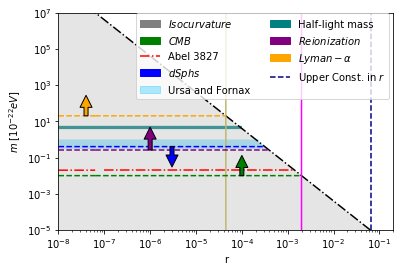
Figure 1: Isocurvature constraints for the SFDM candidate.

These results are important given that laldm demonstrated that an ultra-light axion-like dark matter candidate must be present during inflation. Then, if $r$ is detected in the near future, it could represent a strong constraint for the axion-like particle model. Notice that if we relax the mechanism under this particle is created or if we add an auto-interacting component, we should expect these restrictions be less effective to the model.

We also plotted the actual upper limit for $r$ in a navy blue dashed-line. By the moment this value is not very restrictive for the model since it represents an upper value for $r$. Nevertheless the information it provides is that masses smaller than $m_{upper}$ – the blue dashed-line and black dot-dashed-line intersection – are allowed by the data. However, masses bigger than $m_{upper}$ cannot be discarded since the only possible way to do it is if $r$ would be detected.

IV.2 Real Self-interacting SFDM Candidate

IV.2.1 Cosmological history

In this section a self-interacting SFDM with a positive interaction is considered. This scenario is described by the general potential

$$V(\phi,|\psi|^{2})=\hat{V}(\phi)+\frac{1}{2}m^{2}\psi^{2}+\frac{1}{4}\lambda\psi^{4},$$ (20)

and fixing again $Q=0$ for the SFDM in equation [14]. In what follows we omit the hat in the potential $\hat{V}(\phi)$ in order to make simpler the lecture of the article. Then, always that appears $V$ must be understood that we are referring to $\hat{V}$.

Notice that for this case $M^{2}=m^{2}+\lambda\psi^{2}$. As we have previously discussed the effective mass of the field after inflation remains constant at $M^{2}=m^{2}+\lambda\psi_{i}^{2}$ until $M\sim H$. Then, depending of each contribution to $M^{2}$, we can have two different dynamics.

Weakly self-interacting regime.- This limit is obtained when the constant term $m^{2}$ dominates, that is when

$$m^{2}\gg\lambda\psi_{i}^{2}.$$ (21)

In this regime it is possible to ignore the autointeracting term in Eq. (14) when the oscillations of the scalar field begins. However, by ignoring this term the field behaves as a free field and from (16) the field value always decreases. Therefore the autointeracting term never dominates and all the cosmological history remains the same as in the pure free SFDM scenario. In fact, thanks to the decreasing behavior of this scenario we can consider that this regime is fulfilled always that $m^{2}\geq\lambda\psi_{i}^{2}$ or equivalently when $\lambda\leq m^{2}/\psi_{i}^{2}$. If the SFDM oscillations start at the same time than in the free case (which is a good approximation since the effective mass of the SFDM is $M^{2}=m^{2}+\lambda\psi^{2}_{i}\leq 2m^{2}$), we observe from (17) that it should be satisfied that

$$\left(\frac{\lambda}{10^{-96}}\right)\leq 0.6\left(\frac{m}{10^{-22}eV}\right)^{5/2}.$$ (22)

In Fig. 2 we plot the weak limit obtained by our approximation. However this overestimates the maximum value of $\lambda$ since the dust-like behavior is obtained when the $\lambda$ term is completely negligible.

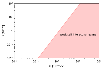
Figure 2: Weakly self-interacting regime

Strong self-interacting regime.- This scenario is obtained when

$$m^{2}\ll\lambda\psi_{i}^{2}.$$ (23)

Here the SFDM follows the dynamical equation (see equation (51) of appendix [A])

$$\frac{1}{\psi^{2}}-\frac{1}{\psi_{0}^{2}}=2\lambda\int_{\phi}^{\phi_{0}}\frac{d\phi}{V_{,\phi}},$$ (24)

where subindex $0$ means quantities at the beginning of the inflationary period. Notice that if the inflationary process does not last for long enough time –meaning that $\psi_{0}^{-2}$ is much smaller than the right hand side value of the above expression–, the SFDM remains frozen with value $\psi_{0}$, while if it lasts long enough time the SFDM reaches an attractor solution.

Attractor behavior of the SF during inflation.- In the strong self-interacting regime, and after enough time, the SFDM follows the attractor solution (52)

$$\psi_{att}=\left(2\lambda\int_{\phi}^{\phi_{0}}V^{-1}_{,\phi}d\phi\right)^{-1/2},$$ (25)

where $\phi_{0}$ is the value of the inflaton at the beginning of inflation. As we can see from the above expression, whether or not the SFDM reaches the attractor solutions depends entirely on the inflationary process and the value of the self-interacting term of the SFDM. In the above expression we can identify two possible branches:

• $\psi_{att}<m/\sqrt{\lambda}$

  The SFDM follows the attractor solution until $\psi\simeq m/\sqrt{\lambda}$. Then the field reaches $\psi_{i}=m/\sqrt{\lambda}$ for the rest of inflation. Notice that this value corresponds to the upper limit that the weakly self-interacting regime allows. Then the field starts evolving when $H\sim M\simeq m$ behaving as a free SF. In this way the constrictions given in the non-interacting case apply and the initial conditions are also fixed by $\psi_{i}$. Using both relations the $\lambda$ value is approximated

  $$\left(\frac{\lambda}{10^{-96}}\right)\simeq 0.6\left(\frac{g_{*osc}}{3.36}\right)^{3/4}\left(\frac{g_{s*osc}}{3.91}\right)^{-1}\left(\frac{m}{10^{-22}eV}\right)^{5/2}.$$ (26)

  Without lost of generality the mass term and the auto-interacting constant are rescaled by typical values, that is, the mass term is measured in units of $10^{-22}eV$ while the auto-interacting constant in terms of $10^{-96}$.
  

• $\psi_{att}>m/\sqrt{\lambda}$

  In this scenario the dynamics of the inflaton, given by (25), implies that the initial condition of the field after the inflationary period is

  $$\psi_{att}^{i}=\left(2\lambda\int_{\phi_{end}}^{\phi_{0}}V^{-1}_{,\phi}d\phi\right)^{-1/2},$$ (27)

  where $\phi_{end}$ is the value of the inflaton at the end of inflation. We need to stress out that this is the value of the field until its oscillation period starts (i.e. when $M\sim H$).

In this scenario and for $\psi_{att}>m/\sqrt{\lambda}$ (regardless of whether the scalar field reached the attractor behavior or not) we observe that at the time the SFDM starts its oscillations its effective mass is linear in the field. In that regime the scalar field evolves as $\psi\sim 1/a$ and its energy density as $\rho_{\psi}\sim 1/a^{4}$, behaving as radiation. Then, when $m^{2}\sim\lambda\psi_{t}^{2}$ the effective scalar field mass is now constant, obtaining the dust-like behavior already analyzed. Therefore, the history of the scalar field density is

$$\rho_{\psi}=\left\{\begin{array}[]{ll}\frac{1}{4}\lambda\psi_{i}^{4}&\text{when }H^{2}\gg\lambda\psi_{i}^{2}\\ \frac{1}{4}\lambda\psi_{i}^{4}\left(\frac{a_{osc}}{a}\right)^{4}&\text{when }H_{t}^{2}\leq\lambda\psi^{2}\leq H^{2}\\ \frac{1}{2}m^{2}\psi_{t}^{2}\left(\frac{a_{t}}{a}\right)^{3}&\text{when }H^{2}\leq m^{2}\ \text{and}\ \lambda\psi^{2}<m^{2}\end{array}\right.$$ (28)

Here sub-index $t$ means quantities measured at transition between radiation-like to dust-like behavior of the SFDM and

$$\psi_{i}^{2}=\left[\frac{2m^{2}}{\lambda}\psi_{t}^{2}\right]^{1/2}\left(\frac{a_{t}}{a_{osc}}\right)^{2}.$$ (29)

Notice that, for simplicity, we have taken an instantaneous transition between radiation-like to dust-like behaviors.

Since the auto-interacting KG equation cannot be solved exactly we work with approximated solutions. By using a pure approximated description of the system, SFphi42 obtained the relation (see its equation 80 and 86 and also SFphi41 )

$$\left(\frac{a_{t}}{a_{osc}}\right)^{2}=\frac{3}{7^{1/3}f^{2}(\frac{a_{s}}{r_{S}})},$$ (30a)

where

$$f(\sigma)=\frac{1}{s^{1/3}(1+4s)^{1/6}},$$ (30b)

with

$$s=\frac{4\sigma-1+\sqrt{(4\sigma-1)^{2}+12\sigma}}{6}.$$ (30c)

Additionally $r_{S}=2mG/c^{2}$ and $a_{s}=\hbar^{2}\lambda/4\pi m$. Then it follows that $a_{s}/r_{S}=\lambda M_{pl}^{2}/m^{2}$. Rearranging the expression in a more convenient way we have

$$\sigma\simeq 5.93\times 10^{2}\left(\frac{m}{10^{-22}eV}\right)^{-2}\left(\frac{\lambda}{10^{-96}}\right).$$ (31)

Notice that when $a_{t}/a_{osc}\simeq 1$, i.e. $3/(7^{1/3}f^{2}(\sigma))\sim 1$, there is no radiation-like epoch. This scenario should match with the non-interacting scenario that we present previously. Inserting Eq. (30a) into (29) yields to

$$\psi_{i}^{2}=\frac{3}{7^{1/3}f^{2}(\sigma)}\left[\frac{2m^{2}}{\lambda}\psi_{t}^{2}\right]^{1/2}.$$ (32)

The relation (32) matches the field at $\psi_{t}$ with its value right after inflation ends. Then if we obtain the value of $\psi_{t}$ by comparing with quantities at present, with the above expressions we can also obtain the value of $\psi_{i}$. On the other hand, notice that at $a_{t}$ the scalar field behaves as dust with an effective mass $M^{2}=m^{2}+\lambda\psi^{2}_{t}$. This implies that dust-like oscillations of the SF began a little before than in the non-interacting case. If we allow $m$ to start its dust-like behavior during the radiation-dominated Universe and using the fact that $m^{2}$ is about the same order that $\lambda\psi^{2}_{t}$, we get that such oscillations start during the same epoch than in the non-interacting case. In fact because the decreasing behavior of the SF during the dust-like period ($\psi\sim 1/a^{3/2}$) the auto-interacting term contribution quickly vanishes and then the dynamics of the field is described only by the mass term $m$. Thus, once the dust-like behavior starts, the dynamics is described similarly to the non-interacting case, in such case the condition (17) is fulfilled by the SF as well, but interchanging subindex $i$ with $t$.

IV.2.2 Constraints from isocurvature perturbations

As we have shown in the last section we have two different scenarios for this model: a weak self-interacting and a strong self-interacting. In the weak limit our SFDM behaves effectively as a free field without auto-interaction, and in such case the constrictions for the free field apply to this scenario as well. On the other hand when the auto-interacting term is big enough, the SFDM will have a new period with a behavior similar to a radiation-like fluid. In this way the constrictions we obtained before will not apply to this model anymore.

In the strong self-interacting regime, during the inflationary era, the SFDM follows the solution (24). The value the homogeneous field acquired after inflation depends on the amount of time the inflationary process takes place and then the condition $\psi_{att}\lessgtr m/\sqrt{\lambda}\equiv\psi_{t}$ –if the inflationary period is short, then the field $\psi$ remains frozen at value $\psi_{i}\simeq\psi_{0}$, while if it lasts long enough the SFDM reaches the attractor behavior (25)–. If the SFDM reaches the solution (25) and for $\psi_{att}<\psi_{t}$ the field follows the attractor solution until $\psi\simeq\psi_{t}$. Then the SFDM is frozen at that value and starts oscillating as a free field when $m\sim H$. We can constrain this scenario by noticing that it is the same case than the free one but with the initial condition $\psi_{i}=\psi_{t}$. Matching Eq. (17) with $\psi_{t}$ and making use of the constriction (19) we obtain

$$\left(\frac{\lambda}{10^{-96}}\right)\leq 0.6\left(\frac{2\times 10^{-4}}{r}\right)^{5}.$$ (33)

In Fig. 3 we have plotted the above condition that is valid during the strong self-interacting regime, when $\psi_{att}<\psi_{t}$. The pink region corresponds to the region allowed by isocurvature perturbations in this limit. As we observe the self-interacting term for this model can be constrained in a similar way than the mass parameter in the free case. This scenario must fulfill the relation (19) as well, since its cosmological evolution after inflation is only like a free SFDM.

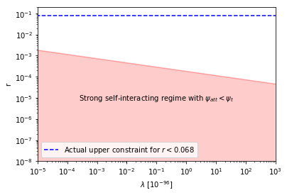
Figure 3: Isocurvature constraints for the strong self-interacting regime with $\psi_{att}<\psi_{t}$.

Additionally, in this scenario, the inflationary potential fulfills the condition

$$\left(\int^{\phi_{0}}_{\phi}V_{,\phi}^{-1}d\phi\right)^{-1/2}<\sqrt{2}m.$$ (34)

We can see that it is very difficult to obtain this relation for an ultra-light SFDM candidate. For example, if we consider a chaotic-like inflationary potential, $V(\phi)=\frac{1}{2}M_{inf}^{2}\phi^{2}$, the above conditions imply that

$$\left(\log\frac{\phi_{0}}{\phi}\right)^{-1/2}<\sqrt{2}\frac{m}{M_{inf}}.$$ (35)

However, for this potential the mass $M_{inf}$ of the inflaton that best matches the observations is of order $M_{inf}\sim 10^{12}GeV$ Liddle . If now we assume an ultra-light SFDM candidate with a mass $m\sim 10^{-22}eV$, given that the cosmological and astrophysical constrictions for this model are the same than in the free case and in this scenario it is necessary to obtain an ultra-light SFDM, the above conditions imply that the logarithmic part of the expression should be lower that $\sim 10^{-43}$. The inflationary behavior for a chaotic-like inflaton ends when $\phi_{end}\simeq 2M_{pl}$ curvatonatractor ; Liddle . Moreover as it is explained in curvatonatractor , the initial condition of the inflaton cannot be arbitrarily large since the stochastic behavior is significant for $\dot{\phi}H^{-1}<H/2\pi$. If the Universe starts when the inflaton escapes from this behavior we have that its initial condition should be

$$\phi_{0}\sim 10^{5}\times M_{pl}\left(\frac{10^{13}GeV}{M_{inf}}\right)^{1/2}.$$ (36)

where we can easily see that the condition given in (35) cannot be fulfilled. In fact if we insert the left part of (35) in equation (24) and by considering the above result and the fact that in this scenario the self-interacting term must be incredible small (see equation (33)) in order to fulfil cosmological and astrophysical constrictions, we can observe that the attractor behavior is not reached when it is assumed a chaotic-like inflationary potential. This implies that if a self-interacting SFDM candidate coexists with the inflaton, and that during the begining of the inflationary period it starts in the strong-field scenario, it should remain within the strong regime since their conditions are easier to satisfy.

If the SFDM reached the solution (25) and when $\psi_{att}>\psi_{t}$ we have that the field follows the attractor solution during all the inflationary period. Hence the initial condition for the SFDM is given by (27)

$$\psi_{att}^{i}=\left(2\lambda\int_{\phi_{end}}^{\phi_{0}}V^{-1}_{,\phi}d\phi\right)^{-1/2}.$$ (37)

Then the SFDM remains frozen at value $\psi_{att}^{i}$ until $M\sim H$ and starts oscillating with a quartic potential. In this scenario the SFDM density behaves as $\rho_{SFDM}\propto\psi^{4}$ and in such case we can write $\delta\rho_{\psi}/\rho_{\psi}=4\delta\psi/\psi_{i}$. Therefore the primordial isocurvature perturbations for a strong self-interacting SFDM is given by

$$P_{SFDM}(k)=\left(\frac{2H_{*}}{\pi\psi_{i}}\right)^{2}.$$ (38)

In the last section we showed the relation of the initial condition with the value of the field today. Using eqs. (32) and (17), with $g_{*osc}=3.36$ and $g_{s*osc}=3.91$ and appropriate units we obtain

$$r<\frac{1.172\times 10^{-4}}{7^{1/3}f^{2}(\sigma)}\left[\frac{2\left(\frac{m}{10^{-22}eV}\right)^{3/2}}{\left(\frac{\lambda}{10^{-96}}\right)}\right]^{1/2}.$$ (39)

Notice that the above relation is independent of whether the SFDM followed the attractor solution or not and therefore the result is general, always that the SFDM remains in the strong self-interacting regime at the end of inflation and its dust-like behavior started in the radiation dominated Universe.

Similarly to the free case, the above relation must be compared with observations in order to get constrictions for the strong self-interacting SFDM scenario.

Other constraints.- In constl1 it was studied the possibility that a SFDM candidate could be self-interacting. In their work they constrain the ratio $\Lambda\equiv m/\lambda^{1/4}$ to be $\Lambda\sim 1eV$ by analyzing the line-of-sight velocity dispersion for the eight dSphs satellites of the Milky Way (MW). This study was complementary to the ones done in SF6 ; constl3 ; constl4 ; constl5 where the SFDM model was studied by using rotational curves of the most Dark Matter dominated galaxies from different surveys and where they obtained the constriction $\Lambda\sim 2.6-2.9eV$. On the other hand, in constl6 the model was studied in a cosmological context by demanding that the SFDM candidate behaves as a dust-like component before the time of matter-radiation equality. In such work they obtain the result $\Lambda>0.8eV$. Finally, it was also possible to test the self-interacting scenario by considering the number of extra relativistic species at BBN. When such observations are confronted with the SFDM it is obtained that it must be fulfilled that $\Lambda\gtrsim 4eV$ (see constl3 ).

In Fig. 4 we have plotted contour levels of the numerical value of the right hand side of the relation (39). The grey region corresponds to values larger than $0.064$ which is the actual upper constraint on tensor-to-scalar ratio. This means that within that region we are certain that (39) is fulfilled and, by the moment, just this region is completely allowed by observations. With this in mind the plot should be understood as follows: let us suppose that in the near future we measure a value for $r$. Such value will coincide with a curve in Fig. 4. Then, the parameter space allowed by data should be the one where the contour levels are bigger than the detected value of $r$, while the one with smaller values in the contour levels must be discarded. Similar to the free case, if $r$ is not detected but it continues with an upper limit, this implies that regions with contour levels bigger than such upper value will be allowed by the data, however regions with smaller values can not be discarded until $r$ is detected.

The $\Lambda$ value that satisfies observations of dSph’s line-of-sight is given by the dot-dashed red line, while the region of parameters necessary for rotational curves is presented in blue. Similar to the plot for the free case (fig. 1) we plotted the cosmological constrictions in purple by drawing a curve that refers to the upper value of $\Lambda$ and an arrow that points out to the valid region from the constriction. We did the same for the observations for BBN but in color fuchsia. The white region corresponds to the weak limit. We can see from Fig. 4 that it is possible to fulfill observations for whichever value for the mass as long as the self-interacting constant is large enough. In other words, for a given mass, the measurement of $r$ can only constrain the self-interacting constant with a lower limit. Isocurvature observations (or equivalently observations on $r$) can also help to impose upper values from other kind of constrictions. As an example let us suppose that we want to be completely sure that the measurements obtained by rotational curves are fulfilled. Then, given the actual upper constraints in $r$, the only region of parameters that we can be sure that fulfills observations are the ones in the blue region that are also inside the gray region.

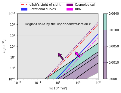
Figure 4: Isocurvature constraints for the strong self-interacting scenario with $\psi_{att}>\psi_{t}$.

Remark: This scenario is of special interest given that it is natural to avoid isocurvature perturbations when the auto-interacting term of the SF is big enough. Additionally, if the SFDM reached the attractor solution it is possible to justify the initial conditions for the SFDM model.

Similarly to the above description we can compute general constraints for the inflationary potential that should generate inflation on these kind of scenarios. First we have that

$$\left(\int^{\phi_{0}}_{\phi}V_{,\phi}^{-1}d\phi\right)^{-1/2}>\sqrt{2}m,$$ (40)

which is very easy to fulfill as we saw in the chaotic-like example. Using isocurvature constriction we also have

$$r<\frac{0.6\times 10^{40}}{\left(\frac{\lambda}{10^{-96}}\right)}\left(\frac{1}{\int_{\phi_{end}}^{\phi_{0}}V_{,\phi}^{-1}d\phi}\right),$$ (41)

that can be satisfied as far as the auto-interacting term and the integral are small enough; for example in the chaotic-like scenario by using (35) and (36) and taking $M_{inf}\simeq 10^{-6}M_{pl}$, we can obtain the constriction

$$\left(\frac{\lambda}{10^{-96}}\right)<\frac{0.3288\times 10^{84}}{r}.$$ (42)

that is easily satisfied for whichever value of $\lambda$ of our interest. If now we compare (27) and (32) we have

$$\left(\int_{\phi_{end}}^{\phi_{0}}V^{-1}_{,\phi}d\phi\right)^{-1}=\frac{6}{7^{1/3}f^{2}(\sigma)}\left(2m^{2}\lambda\psi_{t}^{2}\right)^{1/2}.$$ (43)

This relation is interpreted as follows: consider that the auto-interacting SFDM candidate coexists with the inflaton, and it reached the attractor solution (25), and suppose there are several measurements constraining the mass parameter $m$ as well as the auto-interacting parameter $\lambda$, therefore such constraints are translated into restrictions to the inflationary potential. In order to use the above expression to constraint inflationary potentials, we need to be sure that the term $\psi_{0}^{-2}$ can be ignored in (24) i.e. the right-hand side term in equation (24) is big enough compared with $\psi_{0}^{-2}$.

It is also necessary to be careful that the SFDM does not come to dominate the inflationary period. This is guarantee by demanding that

$$\frac{\lambda}{4}<\frac{H_{*}^{2}M_{pl}^{2}}{\psi_{i}^{4}},$$ (44)

or in terms of (37)

$$\lambda>\left(16H_{*}^{2}M_{pl}^{2}\left(\int_{\phi_{end}}^{\phi_{0}}V_{,\phi}^{-1}d\phi\right)^{2}\right)^{-1}.$$ (45)

Taking the chaotic-like example and using $H_{*}=10^{14}GeV$, we obtain the constriction

$$\frac{\lambda}{10^{-96}}>1.444\times 10^{77}.$$ (46)

Notice that the above expression requires $\lambda>10^{-19}$ and then by considering the cosmological and astrophysical constrictions ($\Lambda\sim O(1)eV$) we should have a mass parameter of order $m\sim 10^{-5}eV$. We have to stress out that (46) is obtained for a chaotic-like potential, then, depending on the inflationary potential we will have different limits allowed for the self-interacting scenario. On the other hand if Eq. (45) is not fulfilled and we remain in the strong-self interacting model it should be necessary to consider a two-field inflationary scenario where the SFDM could obtain a non-negligible dynamics during inflation.

IV.3 Complex SFDM generalization

As we have seen at the beginning of this section, when we consider a complex scalar field its dynamics is modified only by the centrifugal term (see eq. (14)). However as it was mentioned in SFphi42 such term does not affect the dynamics of the field at cosmological levels, obtaining then that a complex scalar field and a real scalar field have the same cosmological history in the Universe. In this way if we take that our complex SFDM fulfills slow-roll conditions during inflation then its constrictions for isocurvature perturbations must be the same than in the real field analogue.

V Discusions and conclusions

In this paper we have studied the possibility that a free or a self-interacting SFDM particle could coexist with the inflaton during inflation. In our assumptions we have considered the SFDM as a spectator in the inflationary process. Then, the SFDM contributes to the primordial spectrum by generating isocurvature perturbations. By using the actual upper constraints in the measurements of the tensor-to-scalar ratio $r$ was possible to test the free parameters for each model. As we discussed, at the moment it is difficult to rule-out some regions of parameters, however it could be possible if $r$ is measured soon.

Our main results are shown in figures 1 and 4. In Fig. 1 we have identified the masses allowed in the free model by isocurvature as well as cosmological and astrophysical observations. We obtained that in order to fulfill the constrictions imposed by CMB we should not detect gravitational waves until $r\simeq 1.3\times 10^{-3}$, while if we were interested in fulfilling all the observations, we should not detect gravitational waves until $r\lesssim 2.33\times 10^{-5}$. This last result is important given that the detectability of gravitational waves could represent a strong constriction for the free model. Analogously, in figure 4 we have plotted in a $m\ -\ \lambda$ plane the region of parameters for the strong-self-interacting model that are allowed by observations. We noticed that for a given mass of the SFDM it is always possible to avoid isocurvature constrictions and fit astrophysical and cosmological observations if a large enough self-interaction is added. Then we notice with this result that the addition of a self-interacting component to the SFDM seems to be a natural solution for the model given that is possible to fulfill naturally all the constrictions that the model has. On the other hand we explain how the SFDM spectator scenario could help to choose the inflationary potential responsible to produce the inflationary period.

VI Acknowledgments

We would like to thank Abril Súarez for discussions on this subject. This work was partially supported by CONACyT México under grants CB-2014-01 No. 240512, Project No. 269652 and Fronteras Project 281; Xiuhcoatl and Abacus clusters at Cinvestav, IPN; I0101/131/07 C-234/07 of the Instituto Avanzado de Cosmología (IAC) collaboration (http://www.iac.edu.mx/). TM is partially supported by Conacyt through the Fondo Sectorial de Investigación para la Educación, grant CB-2014-1, No. 240512. JAV acknowledges the support provided by FOSEC SEP-CONACYT Investigación Básica A1-S-21925, and UNAM-PAPIIT IA102219. LEP was supported by CONACyT México.

Appendix A The attractor behaviour for the SFDM candidate

In this appendix we comment about the attractor behaviour of the strong-self-interacting SFDM during inflation. For this purpose let us remember the dynamical equations that the Universe follows when it contains only two real scalar fields $\phi$ and $\psi$. In that case the Universe is described by the Friedmann and Klein-Gordon differential equations

$$H^{2}=\frac{1}{3M_{pl}^{2}}\left[\frac{1}{2}\dot{\phi}+\frac{1}{2}\dot{\psi}+V(\phi,\psi)\right],$$ (47a)

$$\ddot{\phi}_{i}+3H\dot{\phi}_{i}+V_{,\phi_{i}}=0$$ (47b)

where $\dot{\phi}_{i}\equiv d\phi_{i}/dt$, $V_{,\phi_{i}}\equiv dV/d\phi_{i}$, $M_{pl}=1.221\times 10^{19}GeV$ is the Planck mass and $\phi_{1,2}=\phi,\psi$. In what follows we consider the full potential $V(\phi,\psi)\simeq\hat{V}(\phi)+m^{2}\psi^{2}/2+\lambda\psi^{4}/4$.

In the IS it is assumed that the Universe is dominated by the inflaton and that it is slowly-rolling during that process, i.e. that the slow-roll parameters

$$\epsilon_{\phi}\equiv\frac{M_{pl}^{2}}{2}\left(\frac{V_{,\phi}}{V}\right)^{2},\ \ \ \ \eta_{\phi}\equiv M_{pl}^{2}\left(\frac{V_{,\phi\phi}}{V}\right)$$ (48a)

are small ($$\epsilon_{\phi}\ll 1 \eta_{\phi}\ll 1$$ and ). In that case the Friedmann equation and the Klein-Gordon equation associated to the inflaton are reduced to

$$H^{2}\simeq\frac{\hat{V}(\phi)}{3M_{pl}^{2}},$$ (48b)

$$3H\dot{\phi}+V_{,\phi}=0,$$ (48c)

while the dynamics for the SFDM continue being, in general, described by equation (47b).

A.1 Justifying the slow-roll condition for the SFDM candidate

In order to obtain a slowling-rolling SFDM during the inflationary process it is necessary that it fulfills a similar relation that the one by the inflaton, i.e. the slow-roll parameters associated for the SFDM $\epsilon_{\psi}$ and $\eta_{\psi}$ –defined in a similar way than in (48a)– being small ($\epsilon_{\psi},\eta_{\psi}\ll 1$). Considering that in the IS $V\simeq\hat{V}$ and from (48b) $\hat{V}\simeq 3M_{pl}^{2}H^{2}$ we obtain the slow-roll parameters for the SFDM can be written as

$$\epsilon_{\psi}\simeq\frac{1}{2}\left(\frac{\lambda\psi^{3}}{3M_{pl}H_{*}^{2}}\right)^{2},\ \ \ \ \eta_{\psi}\simeq\frac{\lambda\psi^{2}}{H_{*}^{2}}.$$ (49)

where, as mentioned before, $H_{*}$ is the hubble parameter measured at the epoch of inflation and we have considered that we are in the strong-self-interacting regime. Typically the self-interacting scenario is constrained by the ratio $m/\lambda^{1/4}\sim O(1)eV$ (see subsection IV.1.2 for more detail). As an example, notice that if we consider an ultra-light SFDM candidate with a mass of order $10^{-22}eV$ then the self-interaction should be extremely small $\lambda\sim 10^{-88}$. In that case we can observe that the slow-roll condition can be fulfilled for most of the values of the field $\psi$. However notice that the constraints in this self-interacting scenario allows the SFDM to obtain bigger masses with bigger self-interaction. Then our study is correct always that the slow-roll parameters (49) are small during inflation.

A.2 Attractor solution for the SFDM

The dynamic of the SFDM during inflation is described by equation (48c) but interchanging $\phi$ for $\psi$. In that case notice that both fields must follows the relation

$$\frac{d\psi}{V_{,\psi}}=\frac{d\phi}{V_{,\phi}}$$ (50)

In the strong-self-interacting regime (where $V_{,\psi}\simeq\lambda\psi^{3}$) the above equation results in

$$\frac{1}{\psi^{2}}-\frac{1}{\psi_{0}^{2}}=2\lambda\int_{\phi}^{\phi_{0}}\frac{d\phi}{V_{,\phi}}.$$ (51)

Then, after enough time $\psi$ becomes far smaller than $\psi_{0}$ and then the field reaches the attractor solution

$$\psi_{att}=\left(2\lambda\int_{\phi}^{\phi_{0}}V^{-1}_{,\phi}d\phi\right)^{-1/2},$$ (52)

Notice that the time needed to obtain the attractor behavior for the SFDM is described by the inflationary potential and the self-interaction parameter. Then, the attractor behavior is reached more quickly for the SFDM models with large self-interaction compared to models with small self-interaction. As an example notice that when the SFDM has an extremely small self-interaction and if the inflationary period does not last for a long time, the attractor behavior is not reached and then the dynamics is described by (51). In fact if the self-interaction is extremely small we can approximate $\psi_{end}\sim\psi_{0}$, where $\psi_{end}$ is the value of $\psi$ at the end of inflation.

References

- (1) ]P. A. R. Ade et al. (Planck), Planck 2013 results. XXII. Constraints on inflation, Astron. Astrophys. 571 (2014), A22, arXiv:1303.5082.
- (2) P. A. R. Ade et al. (Planck), Planck 2015 results. XX. Constraints on inflation, arXiv:1502.02114.
- (3) P. A. R. Ade et al. (Planck), Planck 2018 results. X. Constraints on inflation, arXiv:1807.06211.
- (4) D. Barkats et al. (BICEP1), Degree-Scale CMB Polarization Measurements from Three Years of BICEP1 Data, Astrophys. J. 783, 67 (2014), arXiv:1310.1422.
- (5) P. A. R. Ade et al. (BICEP2, Planck), A Joint Analysis of BICEP2/Keck Array and Planck Data, Phys. Rev. Lett. 114 (2015), 101301, arXiv:1502.00612.
- (6) P. A. R. Ade et al. (BICEP2, Keck Array), BICEP2/Keck Array VI: Improved Constraints On Cosmology and Foregrounds When Adding 95 GHz Data From Keck Array, Phys. Rev. Lett. 116 (2016), 031302, arXiv:1510.09217.
- (7) T. Matos and J. A. Nieto, Topics on Kaluza-Klein Theory, Rev. Mex. Fis. 39 (1993), S81.
- (8) T. Matos and F. S. Guzman, Scalar fields as dark matter in spiral galaxies, Class. Quant. Grav. 17 (2000) L9, arXiv:gr-qc/9810028.
- (9) Hu W., Barkana R., Gruzinov A., Fuzzy Cold Dark Matter: The Wave Properties of Ultralight Particles, Physical Review Letters 85 (2000), 1158.
- (10) Bray H., On Dark Matter, Spiral Galaxies, and the Axioms of General Relativity, AMS Contemporary Mathematics Volume. 2013;599(Geometric Analysis, Mathematical Relativity, and Nonlinear Partial Differential Equations), 2010, arXiv:1004.4016.
- (11) Schive H.-Y., Chiueh T., Broadhurst T., Cosmic Structure as the Quantum Interference of a Coherent Dark Wave, Nature Phys. 10 ( 2014a), 496, arXiv:1406.6586.
- (12) Böhmer C. G., Harko T., Can dark matter be a Bose-Einstein condensate?, J. Cosmology Astropart. Phys. 6 (2007), 025, arXiv:0705.4158.
- (13) Marsh D. J. E., Ferreira P. G., Ultra-Light Scalar Fields and the Growth of Structure in the Universe, Phys. Rev. D 82 (2010), 103528, arXiv:1009.3501 [hep-ph].
- (14) Membrado M., Pacheco A. F., Sañudo J., Hartree solutions for the self-Yukawian boson sphere, Phys.Rev. A 39 (1989), 4207.
- (15) Peebles P. J. E., Large-scale background temperature and mass fluctuations due to scale-invariant primeval perturbations, ApJ 263 (1982), L1.
- (16) White S. D. M., Frenk C. S., Davis M., Clusters, Filaments, and Voids in a Universe Dominated by Cold Dark Matter, ApJ 313 (1987), 505.
- (17) Bullock J. S., Boylan-Kolchin M., Small-Scale Challenges to the ?cDM Paradigm, ARAA, 55 (2017), 343, arXiv:1707.04256v1.
- (18) Clowe D., Bradac M., Gonzalez A. H., A Direct Empirical Proof of the Existence of Dark Matter , ApJ 648 (2006), L109, arXiv:astro-ph/0608407.
- (19) Klypin A., Kravtsov A. V., Valenzuela O. Where Are the Missing Galactic Satellites?, ApJ 522 (1999), 82, arXiv:astro-ph/9901240.
- (20) Moore B., Ghigna S., Governato F., Lake G., Quinn T., Stadel J. and Tozzi P., Dark Matter Substructure within Galactic Halos , ApJ 524 (1999), L19, arXiv:astro-ph/9907411.
- (21) Penny S., Conselice C. J., De Rijcke S. and Held E., Hubble Space Telescope survey of the Perseus ClusterI. The structure and dark matter content of cluster dwarf spheroidals, MNRAS 393 (2009), 1054, arXiv:0811.3197.
- (22) J. Magaña and T. Matos, Journal of Physics: Conference Series, Volume 378, conference 1.
- (23) A. Suárez, V. H. Robles, and T. Matos, A Review on the Scalar Field Bose-Einstein Condensate Dark Matter Model, Astrophys. Space Sci. Proc. 38 (2014), 107, arXiv: 1302.0903.
- (24) Marsh D. J. E., Axion cosmology, Phys. Rep. 643 (2016), 1, arXiv:1510.07633 [astro-ph.CO].
- (25) L. Hui, J. P. Ostriker, S. Tremaine, and E. Witten, Ultralight scalars as cosmological dark matter, Phys. Rev. D 95 (2017), 043541, arXiv:1610.08297.
- (26) L. Visinelli, Light axion-like dark matter must be present during inflation, Phys. Rev. D 96 (2017), 023013, arXiv:1703.08798.
- (27) Tommi Markkanen, Arttu Rajantie, and Tommi Tenkanen, Spectator dark matter, Phys. Rev. D 98, 123532 – (2018), arXiv:1811.02586
- (28) Christian T. Byrnes, David Wands, Curvature and isocurvature perturbations from two-field inflation in a slow-roll expansion, Phys.Rev. D 74 (2006), 043529, arXiv:astro-ph/0605679v3.
- (29) J. Alberto Vázquez, Luis E. Padilla, Tonatiuh Matos, Inflationary Cosmology: From Theory to Observations, arXiv:1810.09934.
- (30) D. Lyth, A bound on inflationary energy density from the isotropy of the microwave background, Physics Letters B 147 (1984), 403.
- (31) D. H. Lyth and E. D. Stewart, Constraining the inflationary energy scale from axion cosmology, Physics Letters B 283 (1992), 189.
- (32) E. Madelung, Quantum Theory in Hydrodynamical Form , Zeit. F. Phys. 40 (1927), 322.
- (33) B. Li, T. Rindler-Daller, and P.R. Shapiro, Cosmological constraints on Bose-Einstein-condensed scalar field dark matter, Phys. Rev. D 89 (2014), 083536, arXiv:1310.6061.
- (34) A. Suárez and P. H. Chavanis, Cosmological evolution of a complex scalar field with repulsive or attractive self-interaction, Phys. Rev. D 95 (2017), 063515, arXiv:1608.08624.
- (35) A. Suárez and P.H. Chavanis, Hydrodynamic representation of the Klein-Gordon-Einstein equations in the weak field limit: I. General formalism and perturbations analysis, Phys. Rev. D 92 (2015), 023510, arXiv:1503.07437.
- (36) A. Arbey, J. Lesgourgues and P. Salati, Cosmological constraints on quintessential halos, Phys. Rev. D 65 (2002), 083514, arXiv:astro-ph/0112324.
- (37) J-A. Gu and W-Y. P. Hwang, Can the quintessence be a complex scalar field?, Phys. Lett. B 517 (2001), 1, arXiv:astro-ph/0105099.
- (38) V.A. Belinsky, L.P. Grishchuk, I.M. Khalatnikov and Ya.B. Zeldovich, Inflationary stages in cosmological models with a scalar field, Phys. Lett. B 155(1985), 232.
- (39) T. Piran and R.M. Williams, Inflation in universes with a massive scalar field, Phys. Lett. B 163 (1985), 331.
- (40) T. Kobayashi, R. Murgia, A. De Simone, V. Irs̃ic̃, and M. Viel, Lyman-? constraints on ultralight scalar dark matter: Implications for the early and late universe, Phys. Rev. D 96 (2017), 123514, arXiv:1708.00015.
- (41) K. Harigaya, M. Ibe, M. Kawasaki and T. T. Yanagida, Non-Gaussianity from Attractor Curvaton, Phys. Rev. D 87 (2013), 063514, arXiv:1211.3535.
- (42) Hlozek R., Grin D., Marsh D. J. E., Ferreira P. G., A search for ultra-light axions using precision cosmological data, Phys. Rev. D 91 (2015), 103512, arXiv:1410.2896.
- (43) Paredes A., Michinel H., Interference of Dark Matter Solitons and Galactic Offsets, Physics of the Dark Universe 12 (2016), 50, arXiv:1512.05121.
- (44) A. X. Gonzáles-Morales, D.J.E. Marsh, J. Peñarrubia, and L. Ureña-López, Unbiased constraints on ultralight axion mass from dwarf spheroidal galaxies, Mon. Not. Roy. Astron. Soc. 472 (2017), 1346, arXiv:1609.05856.
- (45) Lora V., Magaña J., Bernal A., Sánchez-Salcedo F. J., Grebel E. K., On the mass of ultra-light bosonic dark matter from galactic dynamics, J. Cosmology Astropart. Phys. 2 (2012), 11, arXiv:1110.2684v2.
- (46) Calabrese E., Spergel D. N., Ultra-light dark matter in ultra-faint dwarf galaxies, MNRAS 460 (2016), 4397, arXiv:1603.07321.
- (47) Sarkar A., Mondal R., Das S., Sethi S. K., Bharadwaj S., Marsh D. J. E., 2016, J. Cosmology Astropart. Phys., 4, 012.
- (48) Armengaud E., Palanque-Delabrouille N., Yèche C., Marsh D. J. E., Baur J., Constraining the mass of light bosonic dark matter using SDSS Lyman- forest, Mon. Not. Roy. Astron. Soc. 471 (2017), 4, arXiv:1703.09126.
- (49) Irs̃ic̃ V., Viel M., Haehnelt M. G., Bolton J. S., Becker G. D., First constraints on fuzzy dark matter from Lyman- forest data and hydrodynamical simulations, Phys. Rev. Lett. 119 (2017), 3, arXiv:1703.04683.
- (50) D. H. Lyth and A. R. Liddle, The primordial density perturbation; cosmology inflation and the origin of structure , 2009, Cambridge University Press.
- (51) Diez-Tejedor A., Gonzáles-Morales A. X., Profumo S., Dwarf spheroidal galaxies and Bose-Einstein condensate dark matter, Phys. Rev. D 90 (2014), 043517, arXiv:1404.1054.
- (52) A. Arbey, J. Lesgourgues and P. Salati, Galactic Halos of Fluid Dark Matter, Phys. Rev. D 68 (2003), 023511, arXiv:astro-ph/0301533.
- (53) T. Harko, Bose-Einstein condensation of dark matter solves the core/cusp problem, JCAP 1105 (2011), 022, arXiv:1105.2996.
- (54) V.H. Robles and T. Matos, Flat Central Density Profile and Constant DM Surface Density in Galaxies from Scalar Field Dark Matter, Mon. Not. Roy. Astron. Soc. 422 (2012), 282, arXiv:1201.3032.
- (55) A. Arbey, J. Lesgourgues and P. Salati, Cosmological constraints on quintessential halos, Phys. Rev. D 65 (2002), 083514, arXiv:astro-ph/0112324.