A nonlinear thermomechanical formulation for anisotropic volume and surface continua

Reza Ghaffari111Corresponding author, email: ghaffari@aices.rwth-aachen.de and Roger A. Sauer222Email: sauer@aices.rwth-aachen.de

Aachen Institute for Advanced Study in Computational Engineering Science (AICES),
RWTH Aachen University, Templergraben 55, 52056 Aachen, Germany

  Abstract: A thermomechanical, polar continuum formulation under finite strains is proposed for anisotropic materials using a multiplicative decomposition of the deformation gradient. First, the kinematics and conservation laws for three dimensional, polar and non-polar continua are obtained. Next, these kinematics are connected to their corresponding counterparts for surface continua based on Kirchhoff-Love kinematics. Likewise, the conservation laws for Kirchhoff-Love shells are derived from their three dimensional counterparts. From this, the weak forms are obtained for three dimensional non-polar continua and Kirchhoff-Love shells. These formulations are expressed in tensorial form so that they can be used in both curvilinear and Cartesian coordinates. They can be used to model anisotropic crystals and soft biological materials, and they can be extended to other field equations, like Maxwell’s equations to model thermo-electro-magneto-mechanical materials.
Keywords: Anisotropic crystals; soft biological materials; three dimensional polar continua; Kirchhoff-Love shells; nonlinear continuum mechanics; thermoelasticity.
 

List of important symbols

$\mathbf{1}$ identity tensor in $\mathbb{R}^{3}$
$\boldsymbol{A}_{\alpha}$ co-variant tangent vectors of $\mathcal{S}_{0}$ at point $\boldsymbol{X}_{\!\text{s}}$ ; $\alpha=1,2$
$\boldsymbol{a}_{\alpha}$ co-variant tangent vectors of $\mathcal{S}$ at point $\boldsymbol{x}_{\text{s}}$ ; $\alpha=1,2$
$\boldsymbol{\mathfrak{a}}_{\alpha}$ co-variant tangent vectors of $\mathcal{S}_{\text{T}}$ at point $\boldsymbol{\mathfrak{X}}_{\text{s}}$ ; $\alpha=1,2$
$\boldsymbol{A}^{\alpha}$ contra-variant tangent vectors of $\mathcal{S}_{0}$ at point $\boldsymbol{X}_{\!\text{s}}$ ; $\alpha=1,2$
$\boldsymbol{a}^{\alpha}$ contra-variant tangent vectors of $\mathcal{S}$ at point $\boldsymbol{x}_{\text{s}}$ ; $\alpha=1,2$
$\boldsymbol{\mathfrak{a}}^{\alpha}$ contra-variant tangent vectors of $\mathcal{S}_{\text{T}}$ at point $\boldsymbol{\mathfrak{X}}_{\text{s}}$ ; $\alpha=1,2$
$A_{\alpha\beta}$ co-variant metric of $\mathcal{S}_{0}$ at point $\boldsymbol{X}_{\!\text{s}}$ ; $\alpha,\beta=1,2$
$a_{\alpha\beta}$ co-variant metric of $\mathcal{S}$ at point $\boldsymbol{x}_{\text{s}}$ ; $\alpha,\beta=1,2$
$\mathfrak{a}_{\alpha\beta}$ co-variant metric of $\mathcal{S}_{\text{T}}$ at point $\boldsymbol{\mathfrak{X}}_{\text{s}}$ ; $\alpha,\beta=1,2$
$A^{\alpha\beta}$ contra-variant metric of $\mathcal{S}_{0}$ at point $\boldsymbol{X}_{\!\text{s}}$ ; $\alpha,\beta=1,2$
$a^{\alpha\beta}$ contra-variant metric of $\mathcal{S}$ at point $\boldsymbol{x}_{\text{s}}$ ; $\alpha,\beta=1,2$
$\mathcal{B}_{0}$, $\mathcal{B}_{\text{T}}$, $\mathcal{B}$ reference, intermediate, current configuration of three dimensional continua
$b_{0\,\alpha\beta}$ co-variant curvature tensor components of $\mathcal{S}_{0}$ at point $\boldsymbol{X}_{\!\text{s}}$ ; $\alpha,\beta=1,2$
$b_{\alpha\beta}$ co-variant curvature tensor components of $\mathcal{S}$ at point $\boldsymbol{x}_{\text{s}}$ ; $\alpha,\beta=1,2$
$b_{0}^{\alpha\beta}$ contra-variant curvature tensor components of $\mathcal{S}_{0}$ at point $\boldsymbol{X}_{\!\text{s}}$ ; $\alpha,\beta=1,2$
$b^{\alpha\beta}$ contra-variant curvature tensor components of $\mathcal{S}$ at point $\boldsymbol{x}_{\text{s}}$ ; $\alpha,\beta=1,2$
$\boldsymbol{b}_{0}$ curvature tensor of $\mathcal{S}_{0}$ at point $\boldsymbol{X}_{\!\text{s}}$
$\boldsymbol{b}$ curvature tensor of $\mathcal{S}$ at point $\boldsymbol{x}_{\text{s}}$
$\boldsymbol{\mathfrak{b}}$ curvature tensor of $\mathcal{S}_{\text{T}}$ at point $\boldsymbol{\mathfrak{X}}_{\text{s}}$
$\boldsymbol{b}^{\flat\lhd}$ pull back of $\boldsymbol{b}$, i.e. $\boldsymbol{b}^{\flat\lhd}=\boldsymbol{F}_{\!\text{s}}^{\text{T}}\,\boldsymbol{b}\,\boldsymbol{F}_{\!\text{s}}$
$\boldsymbol{\mathfrak{b}}^{\flat\lhd(\boldsymbol{F}_{\!\text{sT}})}$ pull back of $\boldsymbol{\mathfrak{b}}$, i.e. $\boldsymbol{\mathfrak{b}}^{\flat\lhd(\boldsymbol{F}_{\!\text{sT}})}=\boldsymbol{F}_{\!\text{sT}}^{\text{T}}\,\boldsymbol{\mathfrak{b}}\,\boldsymbol{F}_{\!\text{sT}}$
$\boldsymbol{c}$ body force couple (per unit mass)
$\boldsymbol{C}_{\text{s}}$ surface right Cauchy–Green tensor
${\boldsymbol{C}}$, ${\boldsymbol{C}}_{\text{e}}$, ${\boldsymbol{C}}_{\text{T}}$ right Cauchy–Green tensor and its elastic and thermal part
$\accentset{\circledast}{\boldsymbol{C}}$, $\accentset{\circledast}{\boldsymbol{C}}_{\!\text{e}}$, $\accentset{\circledast}{\boldsymbol{C}}_{\!\text{T}}$ surface right Cauchy–Green tensor and its elastic and thermal part
$\accentset{\ast}{\boldsymbol{C}}$, $\accentset{\ast}{\boldsymbol{C}}_{\!\text{e}}$, $\accentset{\ast}{\boldsymbol{C}}_{\!\text{T}}$ in-plane surface right Cauchy–Green tensor and its elastic and thermal part
${\mathbb{C}}$ elasticity tensor
${\mathbb{C}}^{\text{L}}$ elasticity tensor (with rearranged order of components)
${\boldsymbol{d}}$ rate of deformation
${\Gamma}_{0\,ij}^{k}$ ($\Gamma_{\text{s}0\,\alpha\beta}^{\gamma}$) Christoffel symbols of the second kind of $\mathcal{B}_{0}$ ($\mathcal{S}_{0}$) ; $i,j,k=1,2,3$ ($\alpha,\beta=1,2$)
${\Gamma}_{ij}^{k}$ ($\Gamma_{\text{s}\,\alpha\beta}^{\gamma}$) Christoffel symbols of the second kind of $\mathcal{B}$ ($\mathcal{S}$) ; $i,j,k=1,2,3$ ($\alpha,\beta=1,2$)
$\mathrm{d}A$ ($\mathrm{d}a$) differential surface element on $\mathcal{S}_{0}$ ($\mathcal{S}$)
$\mathrm{d}S$ ($\mathrm{d}s$) differential surface element on $\mathcal{B}_{0}$ ($\mathcal{B}$)
$\mathrm{d}m$ differential mass element
$\mathrm{d}V$ ($\mathrm{d}v$) differential volume element in $\mathcal{B}_{0}$ ($\mathcal{B}$)
$\mathrm{d}l$ differential line element on $\mathcal{S}$
$\delta\bullet$ variation of $\bullet$
$\delta_{ij},\delta^{i}_{j},\delta_{i}^{j}$ Kronecker delta ; $i,j=1,2,3$
${\boldsymbol{e}}^{(n)}$ generalized Eulerian strain
${\boldsymbol{E}}^{(n)}$ generalized Lagrangian strain
${\boldsymbol{\mathcal{E}}}$ permutation tensor
$\boldsymbol{f}$ body force (per unit mass)
${\boldsymbol{F}}$, ${\boldsymbol{F}}_{\!\text{e}}$, ${\boldsymbol{F}}_{\!\text{T}}$ deformation gradient and its elastic and thermal part
$\boldsymbol{F}_{\!\text{s}}$ in-plane surface deformation gradient of $\mathcal{S}$, i.e. $\boldsymbol{F}_{\!\text{s}}=\accentset{\ast}{\boldsymbol{F}}(\xi=0)$
$\accentset{0}{\boldsymbol{F}}$ surface deformation gradient of $\mathcal{S}$, i.e. $\accentset{0}{\boldsymbol{F}}=\accentset{\circledast}{\boldsymbol{F}}(\xi=0)$
$\accentset{\ast}{\boldsymbol{F}}$, $\accentset{\ast}{\boldsymbol{F}}_{\!\text{e}}$, $\accentset{\ast}{\boldsymbol{F}}_{\!\text{T}}$ in-plane surface deformation gradient of $\accentset{\circledast}{\mathcal{S}}$ and its elastic and thermal part
$\accentset{\circledast}{\boldsymbol{F}}$, $\accentset{\circledast}{\boldsymbol{F}}_{\!\text{e}}$, $\accentset{\circledast}{\boldsymbol{F}}_{\!\text{T}}$ surface deformation gradient of $\accentset{\circledast}{\mathcal{S}}$ and its elastic and thermal part
$\boldsymbol{G}_{i}$ co-variant tangent vectors of $\mathcal{B}_{0}$ at point ${\boldsymbol{X}}$; $i=1,2,3$
$\boldsymbol{g}_{i}$ co-variant tangent vectors of $\mathcal{B}$ at point ${\boldsymbol{x}}$; $i=1,2,3$
$\boldsymbol{\mathfrak{g}}_{i}$ co-variant tangent vectors of $\mathcal{B}_{\text{T}}$ at point $\boldsymbol{\mathfrak{X}}$; $i=1,2,3$
$\accentset{\circledast}{\boldsymbol{G}}_{\alpha}$ co-variant tangent vectors of $\accentset{\circledast}{\mathcal{S}}_{0}$ at point $\accentset{\circledast}{\boldsymbol{X}}$; $\alpha=1,2$
$\accentset{\circledast}{\boldsymbol{g}}_{\alpha}$ co-variant tangent vectors of $\accentset{\circledast}{\mathcal{S}}$ at point $\accentset{\circledast}{\boldsymbol{x}}$; $\alpha=1,2$
$\accentset{\circledast}{\boldsymbol{\mathfrak{g}}}_{\alpha}$ co-variant tangent vectors of $\accentset{\circledast}{\mathcal{S}}_{\text{T}}$ at point $\accentset{\circledast}{\boldsymbol{\mathfrak{X}}}$; $\alpha=1,2$
$\boldsymbol{G}^{i}$ contra-variant tangent vectors of $\mathcal{B}_{0}$ at point ${\boldsymbol{X}}$; $i=1,2,3$
$\boldsymbol{g}^{i}$ contra-variant tangent vectors of $\mathcal{B}$ at point ${\boldsymbol{x}}$; $i=1,2,3$
$\boldsymbol{\mathfrak{g}}^{i}$ contra-variant tangent vectors of $\mathcal{B}_{\text{T}}$ at point $\boldsymbol{\mathfrak{X}}$; $i=1,2,3$
$\accentset{\circledast}{\boldsymbol{G}}^{\alpha}$ contra-variant tangent vectors of $\accentset{\circledast}{\mathcal{S}}_{0}$ at point $\accentset{\circledast}{\boldsymbol{X}}$; $\alpha=1,2$
$\accentset{\circledast}{\boldsymbol{g}}^{\alpha}$ contra-variant tangent vectors of $\accentset{\circledast}{\mathcal{S}}$ at point $\accentset{\circledast}{\boldsymbol{x}}$; $\alpha=1,2$
$\accentset{\circledast}{\boldsymbol{\mathfrak{g}}}^{\alpha}$ contra-variant tangent vectors of $\accentset{\circledast}{\mathcal{S}}_{\text{T}}$ at point $\accentset{\circledast}{\boldsymbol{\mathfrak{X}}}$; $\alpha=1,2$
$G_{ij}$ co-variant metric of $\mathcal{B}_{0}$ at point ${\boldsymbol{X}}$; $i,j=1,2,3$
$g_{ij}$ co-variant metric of $\mathcal{B}$ at point ${\boldsymbol{x}}$; $i,j=1,2,3$
$\mathfrak{g}_{ij}$ co-variant metric of $\mathcal{B}_{\text{T}}$ at point $\boldsymbol{\mathfrak{X}}$; $i,j=1,2,3$
$\accentset{\circledast}{G}_{\alpha\beta}$ co-variant metric of $\accentset{\circledast}{\mathcal{S}}_{0}$ at point $\accentset{\circledast}{\boldsymbol{X}}$; $\alpha,\beta=1,2$
$\accentset{\circledast}{g}_{\alpha\beta}$ co-variant metric of $\accentset{\circledast}{\mathcal{S}}$ at point $\accentset{\circledast}{\boldsymbol{x}}$; $\alpha,\beta=1,2$
$G^{ij}$ contra-variant metric of $\mathcal{B}_{0}$ at point ${\boldsymbol{X}}$; $i,j=1,2,3$
$g^{ij}$ contra-variant metric of $\mathcal{B}$ at point ${\boldsymbol{x}}$; $i,j=1,2,3$
$H_{0}$ mean curvature of $\mathcal{S}_{0}$ at $\boldsymbol{X}_{\!\text{s}}$
$H$ mean curvature of $\mathcal{S}$ at $\boldsymbol{x}_{\text{s}}$
${\boldsymbol{H}}$ $:={\boldsymbol{F}}_{\!\text{T},T}^{-\text{T}}\,{\boldsymbol{C}}\,{\boldsymbol{F}}_{\!\text{T}}^{-\text{T}}$
$\boldsymbol{i}$ surface identity tensor on $\mathcal{S}$
$\boldsymbol{I}$ surface identity tensor on $\mathcal{S}_{0}$
$J_{\text{s}}$ area change between $\mathcal{S}_{0}$ and $\mathcal{S}$
$J_{\text{sT}}$ area change between $\mathcal{S}_{0}$ and $\mathcal{S}_{\text{T}}$
${J}$ volume change between $\mathcal{B}_{0}$ and $\mathcal{B}$
${J}_{\text{T}}$ volume change between $\mathcal{B}_{0}$ and $\mathcal{B}_{\text{T}}$, i.e. ${J}_{\text{T}}={\det}\,{\boldsymbol{F}}_{\!\text{T}}$
${\boldsymbol{k}}$ conductivity tensor
$\kappa_{0}$ ($\kappa$) Gaussian curvature of $\mathcal{S}_{0}$ ($\mathcal{S}$) at $\boldsymbol{X}_{\!\text{s}}$ ($\boldsymbol{x}_{\text{s}}$)
$\kappa_{0\,1}$, $\kappa_{0\,2}$ principal curvatures of $\mathcal{S}_{0}$ at $\boldsymbol{X}_{\!\text{s}}$
$\kappa_{1}$, $\kappa_{2}$ principal curvatures of $\mathcal{S}$ at $\boldsymbol{x}_{\text{s}}$
$\boldsymbol{\kappa}$ curvature change relative to intermediate configuration
$\kappa_{\alpha\beta}$ co-variant components of curvature change relative to intermediate configuration
$\mathcal{K}$ total kinetic energy
$\accentset{\circledast}{\boldsymbol{l}}$ rate of deformation of $\accentset{\circledast}{\mathcal{S}}$
$\accentset{0}{\boldsymbol{l}}$ rate of deformation of $\mathcal{S}$, i.e. $\accentset{0}{\boldsymbol{l}}=\accentset{\circledast}{\boldsymbol{l}}(\xi=0)$
${\boldsymbol{l}}$, ${\boldsymbol{l}}_{\text{e}}$, ${\boldsymbol{l}}_{\text{T}}$ rate of deformation of $\mathcal{B}$ and its elastic and thermal part
$\lambda_{1}$, $\lambda_{2}$ principal surface stretches of $\mathcal{S}$ at $\boldsymbol{x}$
$\lambda_{3}$, $\lambda_{3\,\text{e}}$, $\lambda_{3\,\text{T}}$ stretch along $\boldsymbol{n}$ and its elastic and thermal part
$m_{\nu}$, $m_{\tau}$ bending moment components acting at $\boldsymbol{x}_{\text{s}}\in\partial\mathcal{S}$
$M^{\alpha\beta}$ contra-variant bending moment components
$M^{\alpha\beta}_{0}$ $=J\,M^{\alpha\beta}$
$\boldsymbol{m}_{\text{s}}$ surface moment vector acting at $\boldsymbol{x}_{\text{s}}\in\partial\mathcal{S}$
${\boldsymbol{m}}$ moment vector acting at ${\boldsymbol{x}}\in\partial\mathcal{B}$
$\boldsymbol{\mu}_{\text{s}}$ surface moment tensor
$\bar{\boldsymbol{\mu}}_{\text{s}}$ rotated surface moment tensor, i.e. $\bar{\boldsymbol{\mu}}_{\text{s}}^{\text{T}}=\boldsymbol{n}\times\boldsymbol{\mu}_{\text{s}}^{\text{T}}$
${\bar{\boldsymbol{\mu}}}$ moment tensor
${\bar{\boldsymbol{\mu}}}_{0}$ two-point form of the moment tensor, i.e. ${\bar{\boldsymbol{\mu}}}_{0}={J}\,\boldsymbol{F}_{\!\text{s}}^{-1}\,{\bar{\boldsymbol{\mu}}}$
$\boldsymbol{\mu}_{\text{s}}^{\lhd\sharp}$ pull back of the surface moment tensor, i.e. $\boldsymbol{\mu}_{\text{s}}^{\lhd\sharp}=\boldsymbol{F}_{\!\text{s}}^{-1}\,\boldsymbol{\mu}_{\text{s}}\boldsymbol{F}_{\!\text{s}}^{-\text{T}}$
$N^{\alpha\beta}$ total, contra-variant, in-plane stress components
$\boldsymbol{N}$ surface normal of $\mathcal{S}_{0}$ at $\boldsymbol{X}_{\!\text{s}}$
$\boldsymbol{n}$ surface normal of $\mathcal{S}$ at $\boldsymbol{x}_{\text{s}}$
$\boldsymbol{n}_{\text{T}}$ surface normal of $\mathcal{S}_{\text{T}}$ at $\boldsymbol{\mathfrak{X}}_{\text{s}}$
$\boldsymbol{\mathcal{V}}$ normal vector on $\partial\mathcal{S}_{0}$ or $\partial\mathcal{B}_{0}$
$\nu$ normal vector on $\partial\mathcal{S}$ or $\partial\mathcal{B}$
${\boldsymbol{v}}$ velocity vector
$\mbox{\boldmath$\tau$}_{\!\text{v}}$ tangent vector on $\partial\mathcal{S}$, i.e. $\mbox{\boldmath$\tau$}_{\!\text{v}}=\boldsymbol{n}\times\mbox{\boldmath$\nu$}$
${u}$ ($u_{\text{s}}$) internal energy per unit mass, functional for $\mathcal{B}$ ($\mathcal{S}$)
$\mathcal{U}$ total internal energy
$\xi^{i}$ ($\xi^{\alpha}$) convective coordinates on $\mathcal{B}$ ($\mathcal{S}$); $i=1,2,3$ ($\alpha=1,2$)
$\xi$ thickness coordinate
${\psi}$ ($\psi_{\text{s}}$) Helmholtz free energy per unit mass, functional for $\mathcal{B}$ ($\mathcal{S}$)
${\boldsymbol{P}}$ first Piola-Kirchhoff stress tensor
$\mathcal{P}_{\text{ext}}$ total rate of external mechanical power
${\boldsymbol{q}}$ heat flux vector
${\boldsymbol{Q}}$ pull back of heat flux vector, i.e. ${\boldsymbol{Q}}={\boldsymbol{q}}\,{J}\,{\boldsymbol{F}}^{-\text{T}}$
$\mathcal{Q}$ total rate of heat input
$r$ heat source per unit mass
${\rho}_{0}$ ($\rho_{\text{s0}}$) density $\mathcal{B}_{0}$ ($\mathcal{S}_{0}$) at ${\boldsymbol{X}}$ ($\boldsymbol{X}_{\!\text{s}}$)
${\rho}$ ($\rho_{\text{s}}$) density $\mathcal{B}$ ($\mathcal{S}$) at ${\boldsymbol{x}}$ ($\boldsymbol{x}_{\text{s}}$)
$s_{\text{s}}$ entropy per unit of mass, functional for $\mathcal{S}$
${s}$ entropy per unit of mass, functional for $\mathcal{B}$
$S^{\alpha}$ contra-variant, out-of-plane shear stress components of the Kirchhoff-Love shell
$\boldsymbol{S}_{\text{s}}$ surface second Piola-Kirchhoff stress tensor
${\boldsymbol{S}}$ second Piola-Kirchhoff stress tensor
${\boldsymbol{S}}_{\text{T}}$ pushed forward of ${\boldsymbol{S}}$, i.e. ${\boldsymbol{S}}_{\text{T}}=1/{J}_{\text{T}}\,{\boldsymbol{F}}_{\!\text{T}}\,{\boldsymbol{S}}\,{\boldsymbol{F}}_{\!\text{T}}^{\text{T}}$
$\mathcal{S}_{0}$ reference configuration of the mid-surface
$\mathcal{S}$ current configuration of the mid-surface
$\accentset{\circledast}{\mathcal{S}}$ current configuration of the surface through thickness
$\sigma$ Cauchy stress tensor
$\mbox{\boldmath$\sigma$}_{\text{KL}}$ Cauchy stress tensor of the Kirchhoff-Love shell
$\mbox{\boldmath$\sigma$}_{\text{s}}$ surface Cauchy stress tensor, i.e. $\mbox{\boldmath$\sigma$}_{\text{s}}=\boldsymbol{F}_{\!\text{s}}\,\mbox{\boldmath$\sigma$}_{\text{s}}^{\sharp\lhd}\,\boldsymbol{F}_{\!\text{s}}^{\text{T}}$
$\mbox{\boldmath$\sigma$}_{\text{s}}^{\sharp\lhd}$ pull back of $\mbox{\boldmath$\sigma$}_{\text{s}}$, i.e. $\mbox{\boldmath$\sigma$}_{\text{s}}^{\sharp\lhd}=\displaystyle 2\boldsymbol{F}_{\!\text{sT}}^{-1}\rho_{\text{s0}}\frac{\partial{\psi_{\text{s}}}}{\partial{\boldsymbol{C}_{\text{se}}}}\boldsymbol{F}_{\!\text{sT}}^{-\text{T}}$
$\sigma^{\alpha\beta}$ contra-variant components of $\mbox{\boldmath$\sigma$}_{\text{s}}$ ; $\alpha,\beta=1,2$
$t_{0}$ reference shell thickness
$t$ current shell thickness
$T$ absolute temperature
${\boldsymbol{t}}_{0}$ traction acting on the boundary $\partial\mathcal{B}_{0}$ normal to $\boldsymbol{\mathcal{V}}$
${\boldsymbol{t}}$ traction acting on the boundary $\partial\mathcal{B}$ normal to $\nu$
$\boldsymbol{t}_{\text{s}}$ traction acting on the boundary $\partial\mathcal{S}$ normal to $\nu$
$\tau^{\alpha\beta}$ contra-variant components of the Kirchhoff stress tensor, i.e. $\tau^{\alpha\beta}=J\sigma^{\alpha\beta}$ ; $\alpha,\beta=1,2$
${\boldsymbol{w}}$ spin of $\mathcal{B}$
${\boldsymbol{w}}^{\bowtie}$ angular-velocity vector, i.e. axial vector of ${\boldsymbol{w}}$
$\boldsymbol{X}_{\!\text{s}}$ reference position of a surface point on $\mathcal{S}_{0}$
$\boldsymbol{x}_{\text{s}}$ current position of a surface point on $\mathcal{S}$
$\boldsymbol{\mathfrak{X}}_{\text{s}}$ intermediate position of a surface point on $\mathcal{S}_{\text{T}}$
$\accentset{\circledast}{\boldsymbol{X}}$ reference position of a surface point on $\accentset{\circledast}{\mathcal{S}}_{0}$
$\accentset{\circledast}{\boldsymbol{x}}$ current position of a surface point on $\accentset{\circledast}{\mathcal{S}}$
$\accentset{\circledast}{\boldsymbol{\mathfrak{X}}}$ intermediate position of a surface point on $\accentset{\circledast}{\mathcal{S}}_{{\text{T}}}$
${\boldsymbol{X}}$ reference position of a point in $\mathcal{B}_{0}$
${\boldsymbol{x}}$ current position of a point in $\mathcal{B}$
$\boldsymbol{\mathfrak{X}}$ intermediate position of a point in $\mathcal{B}_{\text{T}}$

1 Introduction

Thermomechanical formulations for thin-walled structures have many applications. Examples from technology are sheet metal forming [1], gas turbine blades [2], cooling systems for circuit boards [3], fatigue of transistors [4], batteries [5], solar cells [6]. Examples from nature are lipid membranes [7] and leaves [8].
These problems can be modeled as three dimensional (3D)333By “3D continua” we mean 3D volumetric continua as opposed to surface continua. or surface continua. The latter can be used to avoid the high computational costs of volumetric finite element formulations (FE), especially if they are described by Kirchhoff-Love shell kinematics. Anisotropic hyperelastic [9, 10, 11, 12, 13, 14], viscoelastic [15, 16, 17, 18, 19] and plastic [20, 21, 22, 23, 24, 25, 26, 27, 28] constitutive laws are well developed for volumetric continua. These material models need to be adapted to their surface counterparts in order to be used in membrane and shell formulations. Therefore the kinematics of surface and volumetric continua need to be connected to extract these sufrace material models. Steigmann [29, 30] derives a membrane and Koiter shell formulation from 3D nonlinear elasticity. Tepole et al. [31] and Roohbakhshan et al. [32] utilize a projection method to extract a membrane constitutive law from the anisotropic 3D biomaterial model of Gasser et al. [33]. This projection method is extended to extract a shell formulation for composite materials and biological tissues by Roohbakhshan and Sauer [34, 35].
There are different approaches to formulate the kinematics of deforming continua in a thermomechanical framework. The total deformation can be additively or multiplicatively decomposed into thermal and mechanical parts. The additive decomposition is widely used in the linear regime [36]. The linear formulation can be extended to a nonlinear one by using the multiplicative decomposition introduced by Kröner [37], Besseling [38] and Lee [39] for plasticity (see A for a discussion on the limitations of the additive decomposition). The multiplicative decomposition of the deformation gradient is used in the current work.
3D thermomechanical formulations are well developed. Steinmann [40] presents a spatial and material framework of thermo-hyper-elastodynamics. Vujošević and Lubarda [41] propose a finite strain, thermoelasticity formulation based on the multiplicative decomposition of the deformation gradient. Constitutive laws for thermoelastic, elastoplastic and biomechanical materials are discussed by Lubarda [42]. The strong ellipticity condition should be satisfied for the stability of material models [43, p. 258] and [44]. The stability and convexity of thermomechanical constitutive laws are considered by Šilhavý [45] and Lubarda [46, 47]. Miehe et al. [48] propose a thermoviscoplasticity framework based on the multiplicative decomposition of elastic and plastic deformations, logarithmic strain and linear, isotropic, thermal expansion.
Membrane and shell formulations tend to have a much lower computational cost in comparison with volumetric formulations. Gurtin and Murdoch [49] propose a tensorial continuum theory for surface continua coupled to bulk continua. Green and Naghdi [50] propose a thermomechanical shell formulation based on Cosserat surfaces. The temperature variation through the thickness is included, and the surface kinematics are connected to their 3D counterparts. However, the multiplicative decomposition of the deformation gradient and the effects of the thermal deformation gradient on the curvature are not considered in their work. Miehe and Apel [51] propose an isotropic elastoplastic solid-shell formulation and compare the additive and multiplicative decompositions of strains. Sahu et al. [7] propose an irreversible thermomechanical shell formulation for lipid membranes. Since those are usually subjected to isothermal conditions, Sahu et al. [7] do not consider the temperature variation, thermal expansion and heat conduction through the thickness. Steigmann [29, 52, 30] investigates the strong ellipticity and stability condition for membrane, shell and volumetric material models.
A shell formulation can be developed based on rotational or rotation-free formulations. Simo and Fox [53] propose a rotation-based, geometrically exact, shell model based on inextensible one-director and Cosserat surfaces. Simo et al. [54] extend the mentioned theory to consider the thickness variation under loading. Rotation-free Kirchhoff-Love and Reissner-Mindlin shell formulations have been proposed based on subdivision surfaces [55, 56, 57]. Kiendl et al. [58] propose a rotation-free, Kirchhoff-Love shell formulation using isogeometric analysis [59]. The formulation of Kiendl et al. [58] is extended for multi patches and nonlinear materials by Kiendl et al. [60, 61], respectively. Duong et al. [62] propose a rotation-free shell formulation based on the curvilinear membranes and shell formulations of Sauer et al. [63] and Sauer and Duong [64]. Schöllhammer and Fries [65] propose a Kirchhoff-Love shell theory based on tangential differential calculus without the introduction of a local coordinate system. See also Duong et al. [62] and Schöllhammer and Fries [65] for recent reviews of shell formulations.
A FE formulation is proposed by Jeffers [66] for heat transfer through shells. FE shell formulations for functionally graded materials are proposed by Reddy and Chin [67], El-Abbasi and Meguid [68], Cinefra et al. [69] and Kar and Panda [70]. Harmel et al. [71] use hybrid finite element discretizations that combine isogeometric and Lagrangian interpolations for accurate and efficient thermal simulations.
Thermomechanical problems can be solved computationally either by monolithic or by splitting methods. In a monolithic approach, which tends to be more robust, the mechanical and thermal parts are assembled in a single matrix and solved together. In splitting methods, the problem is divided into mechanical and thermal parts and each part is solved separately and the results are exchanged between partitions. For the partitioning, either isothermal or adiabatic splits444The adiabatic split becomes the isentropic split if there is no dissipation [72]. can be used. The latter method can be shown to be unconditionally stable [72, 73].
The condition number and accuracy of the numerical method is affected by the discretization method. The influence of the discretization on the condition number of heat conduction problems is investigated by Surana and Orth [74, 75] for shells, and by Ling and Surana [76] for axisymmetric problems. Furthermore, the temperature and flux discontinuity should be considered in the modeling of interfaces [77, 78, 79].
Sauer et al. [80] present the multiplicative decomposition of the surface deformation gradient and examine its consequences on the kinematics, balance laws and constitutive relations of curved surfaces. Their formulation uses a direct surface description in curvilinear coordinates that is not necessarily connected to an underlying 3D volumetric formulation. Their examples consider isotropic material behavior. The present formulation, on the other hand, considers the derivation of surface formulations from 3D theories using a tensorial description and accounting for anisotropic material behavior. In the current work, the kinematics of two and three dimensional continua are connected for nonisothermal materials. This connection can be used to extract membrane and shell material models from their 3D counterparts. In addition, it can be used to extend available isothermal membrane and shell material models [81, 82] to non-isothermal constitutive laws.
The highlights of the current work are:

  • 1.

    The balance laws for surface and 3D continua are connected. So the extraction of the surface constitutive laws from their 3D counterparts becomes clearer.

  • 2.

    A multiplicative decomposition is used to obtain a new nonlinear thermomechanical shell formulation.

  • 3.

    Anisotropy is considered in the thermal expansion, conductivity and Helmholtz free energy.

  • 4.

    The formulation can be used to describe coupled, nonlinear thermomechanical behavior of 2D and 3D crystals, and anisotropic biological materials.

  • 5.

    The proposed thermomechanical formulation is suitable for an extension to a new thermo-electro-magneto-mechanical formulation for surface and 3D continua based on the works of Green and Naghdi [83], Chatzigeorgiou et al. [84], Baghdasaryan and Mikilyan [85], Dorfmann and Ogden [86], Mehnert et al. [87].

  • 6.

    It can be used in the simulation of anisotropic thermal conductivity in printed circuit boards such as discussed in Dede et al. [88, 89].

The remainder of this paper is organized as follows: Different descriptions of tensorial quantities and three tensorial products are introduced in Sec. 2. In Sec. 3, the kinematics and equilibrium relations of a 3D anisotropic polar continua are obtained in curvilinear coordinates. Sec. 3 is closed with simplified anisotropic non-polar continua. In Sec. 4, the Kirchhoff-Love shell formulation is obtained from the proposed 3D formulation. In Sec. 5, the evolution of material symmetry groups and constitutive laws for heat transfer are discussed, and some examples of the Helmholtz free energy are presented. The paper is concluded in Sec. 6.

2 Different description of tensors

In this section, some preliminary descriptions for tensorial objects in the reference and current configurations are discussed. The push forward and pull back operators are introduced for co-variant, contra-variant, and mixed tensors. Further, three tensorial products are introduced. These descriptions and tensorial products are used in the next sections for the development of a thermomechanical formulation. Tensors related to surface continua are indicated555$\bullet$” is a placeholder for general tensorial quantities. by $\bullet_{\text{s}}$ while tensors related to three dimensional continua have no additional subscript. Tensors related to the intermediate configuration are written in Gothic font. The tangent vectors of three dimensional continua and of the shell mid-surface are denoted by $\boldsymbol{G}_{i}$ and $\boldsymbol{A}_{\alpha}$ in the reference configuration and $\boldsymbol{A}_{\alpha}$ and $\boldsymbol{g}_{i}$ in the current configuration. Here, Latin and Greek indexes run from 1 to 3 and 1 to 2, respectively.
The co-variant and contra-variant descriptions for the general vector $\boldsymbol{u}$ in the reference configuration $\mathcal{B}_{0}$ and the general vector $\boldsymbol{v}$ in the current configuration $\mathcal{B}$ are defined as666$\mathcal{B}_{0}$ and $\mathcal{B}$ are the reference and current configuration, see Sec. 3 for details. [43, 90, 91, 92, 93, 94]

$$\begin{array}[]{lllll}\displaystyle{\boldsymbol{u}}^{\sharp}\!\!\!&:=&\!\!\!\displaystyle u^{i}\,\boldsymbol{G}_{i}~{},~{}~{}\displaystyle{\boldsymbol{v}}^{\sharp}\!\!\!&:=&\!\!\!\displaystyle v^{i}\,\boldsymbol{g}_{i}~{},\\[8.53581pt] \displaystyle{\boldsymbol{u}}^{\flat}\!\!\!&:=&\!\!\!\displaystyle u_{i}\,\boldsymbol{G}^{i}~{},~{}~{}\displaystyle{\boldsymbol{v}}^{\flat}\!\!\!&:=&\!\!\!\displaystyle v_{i}\,\boldsymbol{g}^{i}~{},\end{array}$$ (1)

where

$$\begin{array}[]{lllll}\displaystyle u^{i}\!\!\!&=&\!\!\!\displaystyle{\boldsymbol{u}}\cdot\boldsymbol{G}^{i}~{},~{}~{}\displaystyle v^{i}\!\!\!&=&\!\!\!\displaystyle{\boldsymbol{v}}\cdot\boldsymbol{g}^{i}~{},\\[8.53581pt] \displaystyle u_{i}\!\!\!&=&\!\!\!\displaystyle{\boldsymbol{u}}\cdot\boldsymbol{G}_{i}~{},~{}~{}\displaystyle v_{i}\!\!\!&=&\!\!\!\displaystyle{\boldsymbol{v}}\cdot\boldsymbol{g}_{i}~{},\end{array}$$ (2)

are the contra-variant and co-variant components of ${\boldsymbol{u}}$ and ${\boldsymbol{v}}$. The co-variant, contra-variant and mixed tensors for the general second order tensors $\boldsymbol{U}~{}\text{in}~{}\mathcal{B}_{0}$ and $\boldsymbol{V}~{}\text{in}~{}\mathcal{B}$ are defined as

$$\begin{array}[]{lllll}\displaystyle{\boldsymbol{U}}^{\sharp}\!\!\!&:=&\!\!\!\displaystyle U^{ij}\,\boldsymbol{G}_{i}\otimes\boldsymbol{G}_{j}~{},~{}~{}\displaystyle{\boldsymbol{V}}^{\sharp}\!\!\!&:=&\!\!\!\displaystyle V^{ij}\,\boldsymbol{g}_{i}\otimes\boldsymbol{g}_{j}~{},\\[8.53581pt] \displaystyle{\boldsymbol{U}}^{\flat}\!\!\!&:=&\!\!\!\displaystyle U_{ij}\,\boldsymbol{G}^{i}\otimes\boldsymbol{G}^{j}~{},~{}~{}\displaystyle{\boldsymbol{V}}^{\flat}\!\!\!&:=&\!\!\!\displaystyle V_{ij}\,\boldsymbol{g}^{i}\otimes\boldsymbol{g}^{j}~{},\\[8.53581pt] \displaystyle{\boldsymbol{U}}^{\backslash}\!\!\!&:=&\!\!\!\displaystyle U^{i}_{~{}j}\,\boldsymbol{G}_{i}\otimes\boldsymbol{G}^{j}~{},~{}~{}\displaystyle{\boldsymbol{V}}^{\backslash}\!\!\!&:=&\!\!\!\displaystyle V^{i}_{~{}j}\,\boldsymbol{g}_{i}\otimes\boldsymbol{g}^{j}~{},\\[8.53581pt] \displaystyle{\boldsymbol{U}}^{/}\!\!\!&:=&\!\!\!\displaystyle U_{i}^{~{}j}\,\boldsymbol{G}^{i}\otimes\boldsymbol{G}_{j}~{},~{}~{}\displaystyle{\boldsymbol{V}}^{/}\!\!\!&:=&\!\!\!\displaystyle V_{i}^{j}\,\boldsymbol{g}^{i}\otimes\boldsymbol{g}_{j}~{},\end{array}$$ (3)

where

$$\begin{array}[]{lllll}\displaystyle U^{ij}\!\!\!&=&\!\!\!\boldsymbol{G}^{i}\cdot{\boldsymbol{U}}\,\boldsymbol{G}^{j}~{},~{}~{}V^{ij}\!\!\!&=&\!\!\!\boldsymbol{g}^{i}\cdot{\boldsymbol{V}}\,\boldsymbol{g}^{j}~{},\\[8.53581pt] \displaystyle U_{ij}\!\!\!&=&\!\!\!\boldsymbol{G}_{i}\cdot{\boldsymbol{U}}\,\boldsymbol{G}_{j}~{},~{}~{}V_{ij}\!\!\!&=&\!\!\!\boldsymbol{g}_{i}\cdot{\boldsymbol{V}}\,\boldsymbol{g}_{j}~{},\\[8.53581pt] \displaystyle U^{i}_{~{}j}\!\!\!&=&\!\!\!\displaystyle\boldsymbol{G}^{i}\cdot{\boldsymbol{U}}\,\boldsymbol{G}_{j}~{},~{}~{}\displaystyle V^{i}_{~{}j}\!\!\!&=&\!\!\!\displaystyle\boldsymbol{g}^{i}\cdot{\boldsymbol{V}}\,\boldsymbol{g}_{j}~{},\\[8.53581pt] \displaystyle\displaystyle U_{i}^{~{}j}\!\!\!&=&\!\!\!\displaystyle\,\boldsymbol{G}_{i}\cdot{\boldsymbol{U}}\,\boldsymbol{G}^{j}~{},~{}~{}\displaystyle V_{i}^{j}\!\!\!&=&\!\!\!\displaystyle\,\boldsymbol{g}_{i}\cdot{\boldsymbol{V}}\,\boldsymbol{g}^{j}~{},\end{array}$$ (4)

are the contra-variant, co-variant and mixed components of ${\boldsymbol{U}}$ and ${\boldsymbol{V}}$. Further, $\boldsymbol{G}^{i}$ and $\boldsymbol{g}^{i}$ are the tangent and dual vectors in the reference and current configuration (see Sec. 3 for their definition). The components of surface tensors can be defined similarly, e.g. $\boldsymbol{U}_{\!\text{s}}^{\sharp}=U^{\alpha\beta}\,\boldsymbol{A}_{\alpha}\otimes\boldsymbol{A}_{\beta}$ with $U^{\alpha\beta}=\boldsymbol{A}^{\alpha}\cdot\boldsymbol{U}\cdot\boldsymbol{A}^{\beta}$. The vectors and tensors defined in Eq. (1) and (3) are just different expressions of the same objects, i.e.  ${\boldsymbol{u}}={\boldsymbol{u}}^{\sharp}={\boldsymbol{u}}^{\flat}$, ${\boldsymbol{v}}={\boldsymbol{v}}^{\sharp}={\boldsymbol{v}}^{\flat}$, ${\boldsymbol{U}}={\boldsymbol{U}}^{\sharp}={\boldsymbol{U}}^{\flat}={\boldsymbol{U}}^{\backslash}={\boldsymbol{U}}^{/}$ and ${\boldsymbol{V}}={\boldsymbol{V}}^{\sharp}={\boldsymbol{V}}^{\flat}={\boldsymbol{V}}^{\backslash}={\boldsymbol{V}}^{/}$. The importance of these descriptions becomes clear when the push forward and pull back operators are defined. The push forward operators for different forms of ${\boldsymbol{U}}$ are defined as

$$\begin{array}[]{lllll}\displaystyle{\boldsymbol{U}}^{\sharp\rhd}\!\!\!&:=&\!\!\!\displaystyle{\boldsymbol{F}}\,{\boldsymbol{U}}^{\sharp}\,{\boldsymbol{F}}^{\text{T}}\!\!\!&=&\!\!\!U^{ij}\,\boldsymbol{g}_{i}\otimes\boldsymbol{g}_{j}~{},\\[8.53581pt] \displaystyle{\boldsymbol{U}}^{\flat\rhd}\!\!\!&:=&\!\!\!\displaystyle{\boldsymbol{F}}^{-\text{T}}\,{\boldsymbol{U}}^{\flat}\,{\boldsymbol{F}}^{-1}\!\!\!&=&\!\!\!U_{ij}\,\boldsymbol{g}^{i}\otimes\boldsymbol{g}^{j}~{},\\[8.53581pt] \displaystyle{\boldsymbol{U}}^{\backslash\rhd}\!\!\!&:=&\!\!\!\displaystyle{\boldsymbol{F}}\,{\boldsymbol{U}}^{\backslash}\,{\boldsymbol{F}}^{-1}\!\!\!&=&\!\!\!U^{i}_{~{}j}\,\boldsymbol{g}_{i}\otimes\boldsymbol{g}^{j}~{},\\[8.53581pt] \displaystyle{\boldsymbol{U}}^{/\rhd}\!\!\!&:=&\!\!\!\displaystyle{\boldsymbol{F}}^{-\text{T}}\,{\boldsymbol{U}}^{/}\,{\boldsymbol{F}}^{\text{T}}\!\!\!&=&\!\!\!U_{i}^{~{}j}\,\boldsymbol{g}^{i}\otimes\boldsymbol{g}_{j}~{},\end{array}$$ (5)

and the pull back operators for different forms of ${\boldsymbol{V}}$ are defined as

$$\begin{array}[]{lllll}\displaystyle{\boldsymbol{V}}^{\sharp\lhd}\!\!\!&:=&\!\!\!\displaystyle{\boldsymbol{F}}^{-1}\,{\boldsymbol{V}}^{\sharp}\,{\boldsymbol{F}}^{-\text{T}}\!\!\!&=&\!\!\!V^{ij}\,\boldsymbol{G}_{i}\otimes\boldsymbol{G}_{j}~{},\\[8.53581pt] \displaystyle{\boldsymbol{V}}^{\flat\lhd}\!\!\!&:=&\!\!\!\displaystyle{\boldsymbol{F}}^{\text{T}}\,{\boldsymbol{V}}^{\flat}\,{\boldsymbol{F}}\!\!\!&=&\!\!\!V_{ij}\,\boldsymbol{G}^{i}\otimes\boldsymbol{G}^{j}~{},\\[8.53581pt] \displaystyle{\boldsymbol{V}}^{\backslash\lhd}\!\!\!&:=&\!\!\!\displaystyle{\boldsymbol{F}}^{-1}\,{\boldsymbol{V}}^{\backslash}\,{\boldsymbol{F}}\!\!\!&=&\!\!\!V^{i}_{~{}j}\,\boldsymbol{G}_{i}\otimes\boldsymbol{G}^{j}~{},\\[8.53581pt] \displaystyle{\boldsymbol{V}}^{/\lhd}\!\!\!&:=&\!\!\!\displaystyle{\boldsymbol{F}}^{\text{T}}\,{\boldsymbol{V}}^{/}\,{\boldsymbol{F}}^{-\text{T}}\!\!\!&=&\!\!\!V_{i}^{j}\,\boldsymbol{G}^{i}\otimes\boldsymbol{G}_{j}~{},\end{array}$$ (6)

where ${\boldsymbol{F}}$ is the gradient deformation (see Sec. 3 for details). It should be noted that the different forms of the push forward of ${\boldsymbol{U}}$ as well as the different forms for the pull back of ${\boldsymbol{V}}$, are not equal in general, i.e.  ${\boldsymbol{U}}^{\sharp\rhd}\neq{\boldsymbol{U}}^{\flat\rhd}\neq{\boldsymbol{U}}^{\backslash\rhd}\neq{\boldsymbol{U}}^{/\rhd}$ and ${\boldsymbol{V}}^{\sharp\rhd}\neq{\boldsymbol{V}}^{\flat\rhd}\neq{\boldsymbol{V}}^{\backslash\rhd}\neq{\boldsymbol{V}}^{/\rhd}$. ${\boldsymbol{F}}$ and its transpose, inverse and transpose-inverse can be written as [95]

$$\begin{array}[]{l}\displaystyle{\boldsymbol{F}}=\boldsymbol{g}_{i}\otimes\boldsymbol{G}^{i}~{},~{}~{}{\boldsymbol{F}}^{\text{T}}=\boldsymbol{G}^{i}\otimes\boldsymbol{g}_{i}~{},~{}~{}{\boldsymbol{F}}^{-1}=\boldsymbol{G}_{i}\otimes\boldsymbol{g}^{i}~{},~{}~{}{\boldsymbol{F}}^{-\text{T}}=\displaystyle\boldsymbol{g}^{i}\otimes\boldsymbol{G}_{i}~{}.\end{array}$$ (7)

In Eq. (6) and (7), the push forward and pull back are defined using ${\boldsymbol{F}}$. They can also be defined with other two-point tensors. The push forward and pull back with the general two-point tensor $\bullet$ are indicated by superscripts $\displaystyle\rhd(\bullet)$ and $\displaystyle\lhd(\bullet)$. Furthermore, similar transformations can be defined for surface objects by replacing the deformation gradient ${\boldsymbol{F}}$ with the surface deformation gradient $\boldsymbol{F}_{\!\text{s}}$ (see Secs. 4.4.4, 4.4.5 and 4.5).
The multiplication operators777Kintzel and Başar [96] and Kintzel [94] use $\times$ instead of $\oplus$. $\otimes$ , $\oplus$ and $\boxtimes$ are defined for two second order tensors ${\boldsymbol{A}}$ and ${\boldsymbol{B}}$ as

$$\begin{array}[]{lll}{\boldsymbol{A}}\otimes{\boldsymbol{B}}\!\!\!&:=&\!\!\!A^{ij}\,B^{kl}\,\boldsymbol{G}_{i}\otimes\boldsymbol{G}_{j}\otimes\boldsymbol{G}_{k}\otimes\boldsymbol{G}_{l}~{},\\ {\boldsymbol{A}}\oplus{\boldsymbol{B}}\!\!\!&:=&\!\!\!A^{ij}\,B^{kl}\,\boldsymbol{G}_{i}\otimes\boldsymbol{G}_{k}\otimes\boldsymbol{G}_{l}\otimes\boldsymbol{G}_{j}=A^{il}\,B^{jk}\,\boldsymbol{G}_{i}\otimes\boldsymbol{G}_{j}\otimes\boldsymbol{G}_{k}\otimes\boldsymbol{G}_{l}~{},\\ {\boldsymbol{A}}\boxtimes{\boldsymbol{B}}\!\!\!&:=&\!\!\!A^{ij}\,B^{kl}\,\boldsymbol{G}_{i}\otimes\boldsymbol{G}_{k}\otimes\boldsymbol{G}_{j}\otimes\boldsymbol{G}_{l}=A^{ik}\,B^{jl}\,\boldsymbol{G}_{i}\otimes\boldsymbol{G}_{j}\otimes\boldsymbol{G}_{k}\otimes\boldsymbol{G}_{l}~{}.\end{array}$$ (8)

The second derivative of a scaler function can then be written as

$$\begin{array}[]{lll}\displaystyle{\mathbb{C}}^{\mathrm{L}}\!\!\!&:=&\!\!\!\displaystyle\frac{\partial^{2}{{\psi}}}{\partial{\boldsymbol{C}}\oplus\partial{\boldsymbol{C}}}=\frac{\partial^{2}{{\psi}}}{\partial{C_{ij}}\partial{C_{kl}}}\,\boldsymbol{G}_{i}\otimes\boldsymbol{G}_{k}\otimes\boldsymbol{G}_{l}\otimes\boldsymbol{G}_{j}~{},\end{array}$$ (9)

or

$$\begin{array}[]{lll}\displaystyle{\mathbb{C}}\!\!\!&:=&\!\!\!\displaystyle\frac{\partial^{2}{{\psi}}}{\partial{\boldsymbol{C}}\otimes\partial{\boldsymbol{C}}}=\frac{\partial^{2}{{\psi}}}{\partial{C_{ij}}\partial{C_{kl}}}\,\boldsymbol{G}_{i}\otimes\boldsymbol{G}_{j}\otimes\boldsymbol{G}_{k}\otimes\boldsymbol{G}_{l}~{}.\end{array}$$ (10)

${\mathbb{C}}$ and $\displaystyle\bigl{(}{\mathbb{C}}^{\mathrm{L}}\bigr{)}^{\text{R}}$ are connected by [96]

$$\begin{array}[]{lll}{\mathbb{C}}\!\!\!&:=&\!\!\!\displaystyle\bigl{(}{\mathbb{C}}^{\mathrm{L}}\bigr{)}^{\text{R}}=\bigl{(}C^{\mathrm{L}\,ijkl}\,\boldsymbol{G}_{i}\otimes\boldsymbol{G}_{j}\otimes\boldsymbol{G}_{k}\otimes\boldsymbol{G}_{l}\bigr{)}^{\text{R}}=C^{\mathrm{L}\,iklj}\,\boldsymbol{G}_{i}\otimes\boldsymbol{G}_{j}\otimes\boldsymbol{G}_{k}\otimes\boldsymbol{G}_{l}~{},\end{array}$$ (11)

where $C^{\mathrm{L}\,iklj}$ can be written as

$$\begin{array}[]{lll}C^{\mathrm{L}\,iklj}\!\!\!&=&\!\!\!\boldsymbol{G}^{i}\otimes\boldsymbol{G}^{j}:{\mathbb{C}}:\boldsymbol{G}^{k}\otimes\boldsymbol{G}^{l}~{}.\end{array}$$ (12)

The rearrangement operators $(\bullet)^{\text{R}}$ and $(\bullet)^{\text{L}}$ cancel each other, i.e.

$$\begin{array}[]{lll}\left[(\bullet)^{\text{R}}\right]^{\text{L}}=\left[(\bullet)^{\text{L}}\right]^{\text{R}}\!\!\!&=&\!\!\!(\bullet)~{}.\end{array}$$ (13)

For different products of ${\boldsymbol{A}}$ and ${\boldsymbol{B}}$, $(\dots)^{\text{R}}$ can be written as [82]

$$\begin{array}[]{lll}({\boldsymbol{A}}\oplus{\boldsymbol{B}})^{\text{R}}\!\!\!&=&\!\!\!{\boldsymbol{A}}\otimes{\boldsymbol{B}}~{},\\[5.69054pt] ({\boldsymbol{A}}\otimes{\boldsymbol{B}})^{\text{R}}\!\!\!&=&\!\!\!{\boldsymbol{A}}\boxtimes{\boldsymbol{B}}^{\text{T}}~{},\\[5.69054pt] ({\boldsymbol{A}}\boxtimes{\boldsymbol{B}})^{\text{R}}\!\!\!&=&\!\!\!{\boldsymbol{A}}\oplus{\boldsymbol{B}}^{\text{T}}~{}.\end{array}$$ (14)

The derivative of a tensor with respect to another tensor can be written as

$$\begin{array}[]{lll}\displaystyle\frac{\partial{\boldsymbol{A}}}{\partial{\boldsymbol{B}}}\!\!\!&:=&\!\!\!\displaystyle\frac{\partial A^{ij}}{\partial B_{kl}}\,\boldsymbol{G}_{i}\otimes\boldsymbol{G}_{j}\otimes\boldsymbol{G}_{k}\otimes\boldsymbol{G}_{l}~{},\end{array}$$ (15)

or

$$\begin{array}[]{lll}\displaystyle\frac{\partial{\boldsymbol{A}}}{\oplus\partial{\boldsymbol{B}}}\!\!\!&:=&\!\!\!\displaystyle\frac{\partial A^{ij}}{\partial B_{kl}}\,\boldsymbol{G}_{i}\otimes\boldsymbol{G}_{k}\otimes\boldsymbol{G}_{l}\otimes\boldsymbol{G}_{j}~{},\end{array}$$ (16)

and they are connected by

$$\begin{array}[]{lll}\displaystyle\frac{\partial{\boldsymbol{A}}}{\partial{\boldsymbol{B}}}\!\!\!&=&\!\!\!\displaystyle\left(\displaystyle\frac{\partial{\boldsymbol{A}}}{\oplus\partial{\boldsymbol{B}}}\right)^{\text{R}}~{}.\end{array}$$ (17)

3 3D volumetric continua

In this section, the kinematics of deforming 3D continua are discussed in a curvilinear coordinate system. Then, the conservation laws are obtained for 3D anisotropic polar continua. Finally, the relations are simplified for anisotropic non-polar thermoelastic materials.

3.1 Curvilinear description of deforming 3D continua

The parametric description of a 3D continua in the reference and current configuration can be written as

$$\begin{array}[]{lllll}{\boldsymbol{X}}\!\!\!&=&\!\!\!{\boldsymbol{X}}(\xi^{i})~{},\quad{\boldsymbol{x}}\!\!\!&=&\!\!\!{\boldsymbol{x}}(\xi^{i},t)~{},\end{array}$$ (18)

where $\xi^{i}$ are the curvilinear parametric coordinates and $t$ denotes time. The tangent vectors are then given by

$$\begin{array}[]{lllll}\boldsymbol{G}_{i}\!\!\!&=&\!\!\!\displaystyle{\boldsymbol{X}}_{\!,i}~{},\quad\boldsymbol{g}_{i}\!\!\!&=&\!\!\!\displaystyle{\boldsymbol{x}}_{,i}~{}.\end{array}$$ (19)

where $\bullet_{,i}=\partial\bullet/\partial\xi^{i}$ is the parametric derivative of $\bullet$. The co-variant metric of the reference and current configuration is defined by the inner product of the tangent vectors by

$$\begin{array}[]{lllll}G_{ij}\!\!\!&=&\!\!\!\boldsymbol{G}_{i}\cdot\boldsymbol{G}_{j}~{},\quad g_{ij}\!\!\!&=&\!\!\!\boldsymbol{g}_{i}\cdot\boldsymbol{g}_{j}~{},\end{array}$$ (20)

and the contra-variant metric is connected to the co-variant metric by

$$\begin{array}[]{lllll}G^{ij}\!\!\!&=&\!\!\![G_{ij}]^{-1}~{},\quad g^{ij}\!\!\!&=&\!\!\![g_{ij}]^{-1}~{},\end{array}$$ (21)

where $[\bullet]^{-1}$ is the inverse operator and $[\bullet]$ indicates the component matrix of $\bullet$. The dual vectors are connected to the tangent vectors by

$$\begin{array}[]{lllll}\boldsymbol{G}^{i}\!\!\!&=&\!\!\!G^{ij}\,\boldsymbol{G}_{j}~{},\quad\boldsymbol{g}^{i}\!\!\!&=&\!\!\!g^{ij}\,\boldsymbol{g}_{j}~{},\end{array}$$ (22)

and the inner product of the tangent and dual vectors are

$$\begin{array}[]{lllll}\delta_{i}^{j}\!\!\!&=&\!\!\!\boldsymbol{G}_{i}\cdot\boldsymbol{G}^{j}~{},\quad\delta_{i}^{j}\!\!\!&=&\!\!\!\boldsymbol{g}_{i}\cdot\boldsymbol{g}^{j}~{},\end{array}$$ (23)

where $\delta_{i}^{j}$ is Kronecker delta. The 3D identity tensor $\boldsymbol{1}$ can be written as

$$\begin{array}[]{lllllllll}\boldsymbol{1}\!\!\!&=&\!\!\!G_{ij}\,\boldsymbol{G}^{i}\otimes\boldsymbol{G}^{j}\!\!\!&=&\!\!\!G^{ij}\,\boldsymbol{G}_{i}\otimes\boldsymbol{G}_{j}\!\!\!&=&\!\!\!\boldsymbol{G}^{i}\otimes\boldsymbol{G}_{i}\!\!\!&=&\!\!\!\boldsymbol{G}_{i}\otimes\boldsymbol{G}^{i}\\ \end{array}$$ (24)

and

$$\begin{array}[]{lllllllll}\boldsymbol{1}\!\!\!&=&\!\!\!g_{ij}\,\boldsymbol{g}^{i}\otimes\boldsymbol{g}^{j}\!\!\!&=&\!\!\!g^{ij}\,\boldsymbol{g}_{i}\otimes\boldsymbol{g}_{j}\!\!\!&=&\!\!\!\boldsymbol{g}^{i}\otimes\boldsymbol{g}_{i}\!\!\!&=&\!\!\!\boldsymbol{g}_{i}\otimes\boldsymbol{g}^{i}~{},\end{array}$$ (25)

such that ${\boldsymbol{U}}=\boldsymbol{1}\cdot{\boldsymbol{U}}={\boldsymbol{U}}\cdot\boldsymbol{1}$ and ${\boldsymbol{V}}=\boldsymbol{1}\cdot{\boldsymbol{V}}={\boldsymbol{V}}\cdot\boldsymbol{1}$. The gradient operator for a general scalar, vector (first order tensor) and second order tensor in the reference and current configuration are

$$\begin{array}[]{lllll}{\text{Grad}}\,\Phi\!\!\!&:=&\!\!\!\Phi_{,i}\,\boldsymbol{G}^{i}~{},\\[8.53581pt] {\text{Grad}}\,{\boldsymbol{u}}\!\!\!&:=&\!\!\!{\boldsymbol{u}}_{,j}\otimes\boldsymbol{G}^{j}\!\!\!&=&\!\!\!u^{i}_{\|j}\,\boldsymbol{G}_{i}\otimes\boldsymbol{G}^{j}~{},\\[8.53581pt] {\text{Grad}}\,{\boldsymbol{U}}\!\!\!&:=&\!\!\!{\boldsymbol{U}}_{\!,k}\otimes\boldsymbol{G}^{k}\!\!\!&=&\!\!\!U^{ij}_{~{}\|k}\,\boldsymbol{G}_{i}\otimes\boldsymbol{G}_{j}\otimes\boldsymbol{G}^{k}{}\\ \end{array}$$ (26)

and

$$\begin{array}[]{lllll}{\text{grad}}\,\Phi\!\!\!&:=&\!\!\!\Phi_{,i}\,\boldsymbol{g}^{i}~{},\\[8.53581pt] {\text{grad}}\,{\boldsymbol{v}}\!\!\!&:=&\!\!\!{\boldsymbol{v}}_{,j}\otimes\boldsymbol{g}^{j}\!\!\!&=&\!\!\!v^{i}_{|j}\,\boldsymbol{g}_{i}\otimes\boldsymbol{g}^{j}~{},\\[8.53581pt] {\text{grad}}\,{\boldsymbol{V}}\!\!\!&:=&\!\!\!{\boldsymbol{V}}_{\!,k}\otimes\boldsymbol{g}^{k}\!\!\!&=&\!\!\!V^{ij}_{~{}~{}|k}\,\boldsymbol{g}_{i}\otimes\boldsymbol{g}_{j}\otimes\boldsymbol{g}^{k}~{},\\ \end{array}$$ (27)

where “$\|$” and “$|$” are the 3D co-variant derivatives in the reference and current configuration, defined by [97]

$$\begin{array}[]{lll}u^{i}_{\|j}\!\!\!&:=&\!\!\!u^{i}_{,j}+u^{k}\,{\Gamma}_{0\,kj}^{i}~{},\\[8.53581pt] U^{ij}_{~{}\,\|k}\!\!\!&:=&\!\!\!U^{ij}_{~{}\,,k}+U^{lj}\,{\Gamma}_{0\,lk}^{i}+U^{il}\,{\Gamma}_{0\,lk}^{j}~{},\\[8.53581pt] v^{i}_{|j}\!\!\!&:=&\!\!\!v^{i}_{,j}+v^{k}\,{\Gamma}_{kj}^{i}~{},\\[8.53581pt] V^{ij}_{~{}~{}|k}\!\!\!&:=&\!\!\!V^{ij}_{~{}~{},k}+V^{lj}\,{\Gamma}_{lk}^{i}+V^{il}\,{\Gamma}_{lk}^{j}~{}.\\[8.53581pt] \end{array}$$ (28)

Here, ${\Gamma}_{ij}^{k}$ and ${\Gamma}_{0\,ij}^{k}$ are the 3D Christoffel symbols of the second kind in the reference and current configuration, defined as

$$\begin{array}[]{lll}{\Gamma}_{0\,ij}^{k}\!\!\!&:=&\!\!\!\boldsymbol{G}_{i,j}\cdot\boldsymbol{G}^{k}{}\end{array}$$ (29)

and

$$\begin{array}[]{lll}{\Gamma}_{ij}^{k}\!\!\!&:=&\!\!\!\boldsymbol{g}_{i,j}\cdot\boldsymbol{g}^{k}~{}.\end{array}$$ (30)

The 3D co-variant derivative of the tangent and dual vector, and the metric in the reference and current configuration are zero (Ricci’s theorem [97, p. 54]), i.e.

$$\begin{array}[]{llllll}\boldsymbol{G}_{i\|j}\!\!\!&=&\!\!\!\boldsymbol{G}_{i,j}-\boldsymbol{G}_{l}\,{\Gamma}_{0\,ij}^{l}=\boldsymbol{0}~{},&\boldsymbol{G}^{i}_{\|j}\!\!\!&=&\!\!\!\boldsymbol{G}^{i}_{,j}+\boldsymbol{G}^{l}\,{\Gamma}_{0\,lj}^{i}=\boldsymbol{0}~{},\\[8.53581pt] G_{ij\|k}\!\!\!&=&\!\!\!0~{},&G^{ij}_{~{}\|k}\!\!\!&=&\!\!\!0\end{array}$$ (31)

and

$$\begin{array}[]{llllll}\boldsymbol{g}_{i|j}\!\!\!&=&\!\!\!\boldsymbol{g}_{i,j}-\boldsymbol{g}_{l}\,{\Gamma}_{ij}^{l}=\boldsymbol{0}~{},&\boldsymbol{g}^{i}_{|j}\!\!\!&=&\!\!\!\boldsymbol{g}^{i}_{,j}+\boldsymbol{g}^{l}\,{\Gamma}_{lj}^{i}=\boldsymbol{0}~{},\\[8.53581pt] g_{ij|k}\!\!\!&=&\!\!\!0~{},&g^{ij}_{~{}\,|k}\!\!\!&=&\!\!\!0~{}.\end{array}$$ (32)

Using Ricci’s theorem, the 3D co-variant derivative can be represented in other arrangements of indices, e.g.

$$\begin{array}[]{lll}\displaystyle U_{ij\|}^{~{}~{}~{}k}\!\!\!&=&\!\!\!\displaystyle G_{il}\,G_{jm}\,G^{kn}\,U^{lm}_{~{}~{}\|n}~{},\\[8.53581pt] \displaystyle V_{ij|}^{~{}~{}k}\!\!\!&=&\!\!\!\displaystyle g_{il}\,g_{jm}\,g^{kn}\,V^{lm}_{~{}~{}~{}|n}~{},\end{array}$$ (33)

where $U_{ij\|}^{~{}~{}~{}k}$ and $V_{ij|}^{~{}~{}k}$ are the contra-variant derivatives. These transformations can be used to define other expressions of the gradient operator. The divergence of a vector and a second order tensor are defined by

$$\begin{array}[]{llllll}{\text{Div}}\,\boldsymbol{u}\!\!\!&:=&\!\!\!\boldsymbol{u}_{,j}\cdot\boldsymbol{G}^{j}=u^{i}_{\|i}~{},&{\text{div}}\,\boldsymbol{v}\!\!\!&:=&\!\!\!\boldsymbol{v}_{,j}\cdot\boldsymbol{g}^{j}=v^{i}_{|i}~{},\\[8.53581pt] {\text{Div}}\,\boldsymbol{U}\!\!\!&:=&\!\!\!\boldsymbol{U}_{\!,j}\cdot\boldsymbol{G}^{j}=U^{ij}_{~{}\|j}\,\boldsymbol{G}_{i}~{},&{\text{div}}\,\boldsymbol{V}\!\!\!&:=&\!\!\!\boldsymbol{V}_{\!,j}\cdot\boldsymbol{g}^{j}=V^{ij}_{~{}~{}|j}\,\boldsymbol{g}_{i}~{}.\\[8.53581pt] \end{array}$$ (34)

With this, the divergence theorem can be used to transfer a domain integral to a boundary integral as

$$\begin{array}[]{lll}\displaystyle\int_{\partial\mathcal{B}_{0}}{{\boldsymbol{u}}\cdot\boldsymbol{\mathcal{V}}\,\mathrm{d}S}\!\!\!&=&\!\!\!\displaystyle\int_{\mathcal{B}_{0}}{{\text{Div}}\,{\boldsymbol{u}}\,\mathrm{d}V}~{},\\[8.53581pt] \displaystyle\int_{\partial\mathcal{B}_{0}}{{\boldsymbol{U}}\,\boldsymbol{\mathcal{V}}\,\mathrm{d}S}\!\!\!&=&\!\!\!\displaystyle\int_{\mathcal{B}_{0}}{{\text{Div}}\,{\boldsymbol{U}}\,\mathrm{d}V{}}\\[8.53581pt] \end{array}$$ (35)

and

$$\begin{array}[]{lll}\displaystyle\int_{\partial\mathcal{B}}{{\boldsymbol{v}}\cdot\mbox{\boldmath$\nu$}\,\mathrm{d}s}\!\!\!&=&\!\!\!\displaystyle\int_{\mathcal{B}}{{\text{div}}\,{\boldsymbol{v}}\,\mathrm{d}v}~{},\\[8.53581pt] \displaystyle\int_{\partial\mathcal{B}}{{\boldsymbol{V}}\,\mbox{\boldmath$\nu$}\,\mathrm{d}s}\!\!\!&=&\!\!\!\displaystyle\int_{\mathcal{B}}{{\text{div}}\,{\boldsymbol{V}}\,\mathrm{d}v}~{},\\[8.53581pt] \end{array}$$ (36)

where $\mathcal{B}_{0}$ and $\mathcal{B}$ are the reference and current configuration of 3D continua and $\partial\mathcal{B}_{0}$ and $\partial\mathcal{B}$ are their corresponding boundaries. $\boldsymbol{\mathcal{V}}$ and $\nu$ are the normal unit vectors on $\partial\mathcal{B}_{0}$ and $\partial\mathcal{B}$.

3.2 Kinematics of deformation

Next, the kinematics of deformation is discussed. An intermediate configuration $\mathcal{B}_{\text{T}}$ is introduced888The deformation of the intermediate configuration can be incompatible [98]., and the reference, intermediate and current configuration $\mathcal{B}_{0}$, $\mathcal{B}_{\text{T}}$ and $\mathcal{B}$ are connected (see Fig. 1).

Refer to caption
Figure 1: Multiplicative deformation decomposition of 3D volumetric continua. $\mathcal{B}_{0}$, $\mathcal{B}_{\text{T}}$ and $\mathcal{B}$ are the reference, intermediate and current configuration and their corresponding tangent vectors are $\boldsymbol{G}_{i}$, $\boldsymbol{\mathfrak{g}}_{i}$ and $\boldsymbol{g}_{i}$. ${\boldsymbol{F}}$, ${\boldsymbol{F}}_{\!\text{T}}$ and ${\boldsymbol{F}}_{\!\text{e}}$ are the total, thermal and elastic deformation gradient.

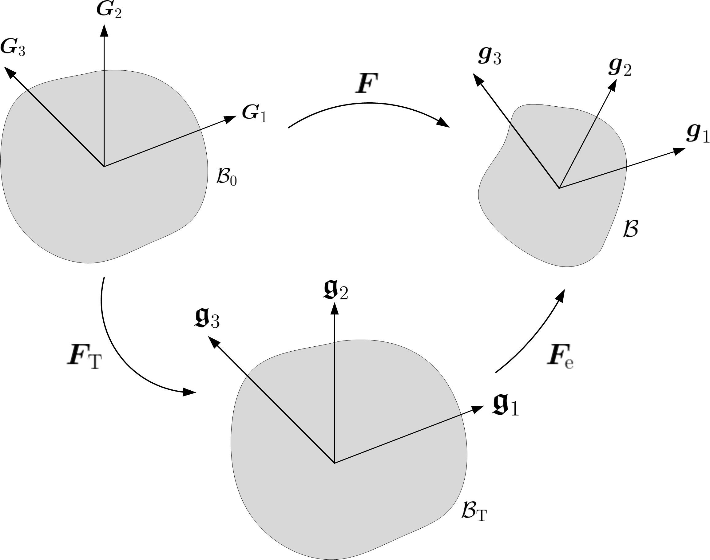
An additive decomposition of the strain should not be used in finite deformations, unless the logarithmic strain is used (see A). The limitation of the additive decomposition of strains is resolved by using a multiplicative decomposition of the deformation gradient. $\mathcal{B}_{0}$ is mapped to $\mathcal{B}$ by ${\boldsymbol{x}}={\boldsymbol{\varphi}}({\boldsymbol{X}})$ and the deformation gradient can be written as (see also Eq. (7))

$$\begin{array}[]{lll}{\boldsymbol{F}}\!\!\!&=&\!\!\!\displaystyle\frac{\partial{{\boldsymbol{x}}}}{\partial{{\boldsymbol{X}}}}=\frac{\partial{{\boldsymbol{x}}}}{\partial{\xi^{i}}}\otimes\frac{\partial{\xi^{i}}}{\partial{{\boldsymbol{X}}}}=\boldsymbol{g}_{i}\otimes~{}\boldsymbol{G}^{i}~{}.\end{array}$$ (37)

It pushes forward the differential line $\mathrm{d}{\boldsymbol{X}}$ to $\mathrm{d}{\boldsymbol{x}}$ as

$$\begin{array}[]{lll}\mathrm{d}{\boldsymbol{x}}\!\!\!&=&\!\!\!\displaystyle{\boldsymbol{F}}\,\mathrm{d}{\boldsymbol{X}}~{},\end{array}$$ (38)

and hence pushes forward $\boldsymbol{G}_{i}$ to $\boldsymbol{g}_{i}$ as

$$\begin{array}[]{lll}\boldsymbol{g}_{i}\!\!\!&=&\!\!\!\displaystyle{\boldsymbol{F}}\,\boldsymbol{G}_{i}~{}.\end{array}$$ (39)

The deformation gradient ${\boldsymbol{F}}$ can be decomposed into the elastic and thermal parts ${\boldsymbol{F}}_{\!\text{e}}$ and ${\boldsymbol{F}}_{\!\text{T}}$ as

$$\begin{array}[]{lll}\displaystyle{\boldsymbol{F}}\!\!\!&=&\!\!\!\displaystyle{\boldsymbol{F}}_{\!\text{e}}\,{\boldsymbol{F}}_{\!\text{T}}~{}.\end{array}$$ (40)

${\boldsymbol{F}}_{\!\text{T}}$ pushes forward $\mathrm{d}\boldsymbol{X}$ to $\mathrm{d}\boldsymbol{\mathfrak{X}}$ as

$$\begin{array}[]{lll}\mathrm{d}\boldsymbol{\mathfrak{X}}\!\!\!&=&\!\!\!{\boldsymbol{F}}_{\!\text{T}}\,\mathrm{d}{\boldsymbol{X}}~{},\end{array}$$ (41)

and hence pushes forward $\boldsymbol{G}_{i}$ to $\boldsymbol{\mathfrak{g}}_{i}$ as

$$\begin{array}[]{lll}\boldsymbol{\mathfrak{g}}_{i}\!\!\!&=&\!\!\!{\boldsymbol{F}}_{\!\text{T}}\,\boldsymbol{G}_{i}~{},\end{array}$$ (42)

where $\mathrm{d}\boldsymbol{\mathfrak{X}}$ and $\boldsymbol{\mathfrak{g}}_{i}$ are the differential line and the tangent vectors of $\mathcal{B}_{\text{T}}$, respectively, and $\boldsymbol{\mathfrak{g}}_{i}$ are defined as

$$\begin{array}[]{lll}\boldsymbol{\mathfrak{g}}_{i}\!\!\!&:=&\!\!\!\boldsymbol{\mathfrak{X}}_{,i}~{}.\end{array}$$ (43)

${\boldsymbol{F}}_{\!\text{e}}$ pushes forward $\mathrm{d}\boldsymbol{\mathfrak{X}}$ to $\mathrm{d}\boldsymbol{x}$ as

$$\begin{array}[]{lll}\mathrm{d}{\boldsymbol{x}}\!\!\!&=&\!\!\!{\boldsymbol{F}}_{\!\text{e}}\,\mathrm{d}\boldsymbol{\mathfrak{X}}~{},\end{array}$$ (44)

and hence pushes forward $\boldsymbol{\mathfrak{g}}_{i}$ to $\boldsymbol{g}_{i}$ as

$$\begin{array}[]{lll}\boldsymbol{g}_{i}\!\!\!&=&\!\!\!{\boldsymbol{F}}_{\!\text{e}}\,\boldsymbol{\mathfrak{g}}_{i}~{}.\end{array}$$ (45)

The right Cauchy-Green deformation tensor ${\boldsymbol{C}}$ and its thermal, ${\boldsymbol{C}}_{\text{T}}$, and elastic, ${\boldsymbol{C}}_{\text{e}}$, parts can be defined as

$$\begin{array}[]{lll}{\boldsymbol{C}}\!\!\!&:=&\!\!\!{\boldsymbol{F}}^{\text{T}}\,{\boldsymbol{F}}={\boldsymbol{F}}_{\!\text{T}}^{\text{T}}\,{\boldsymbol{C}}_{\text{e}}\,{\boldsymbol{F}}_{\!\text{T}}~{},\\[8.53581pt] {\boldsymbol{C}}_{\text{T}}\!\!\!&:=&\!\!\!{\boldsymbol{F}}_{\!\text{T}}^{\text{T}}\,{\boldsymbol{F}}_{\!\text{T}}~{},\\[8.53581pt] {\boldsymbol{C}}_{\text{e}}\!\!\!&:=&\!\!\!{\boldsymbol{F}}_{\!\text{e}}^{\text{T}}\,{\boldsymbol{F}}_{\!\text{e}}~{}.\end{array}$$ (46)

The spatial velocity gradient ${\boldsymbol{l}}$ can be written as

$$\begin{array}[]{lll}\displaystyle{\boldsymbol{l}}\!\!\!&=&\!\!\!\displaystyle\frac{\partial{{\boldsymbol{v}}}}{\partial{{\boldsymbol{x}}}}=\frac{\partial{{\boldsymbol{v}}}}{\partial{{\boldsymbol{X}}}}\,\frac{\partial{{\boldsymbol{X}}}}{\partial{{\boldsymbol{x}}}}=\dot{{\boldsymbol{F}}}\,{\boldsymbol{F}}^{-1}~{},\end{array}$$ (47)

where $\dot{\bullet}$ denotes the material time derivative of $\bullet$, i.e.

$$\begin{array}[]{lll}\displaystyle\dot{\bullet}\!\!\!&=&\!\!\!\displaystyle\frac{\text{D}\bullet}{\text{D}t}=\left.\frac{\partial{\bullet}}{\partial{t}}\right|_{{\boldsymbol{X}}=\text{fixed}}~{},\end{array}$$ (48)

and the velocity ${\boldsymbol{v}}$ is the material time derivative of ${\boldsymbol{x}}$, i.e. ${\boldsymbol{v}}=\dot{{\boldsymbol{x}}}$. ${\boldsymbol{l}}$ can be decomposed into a symmetric (the rate of deformation tensor ${\boldsymbol{d}}$) and skew symmetric (the spin tensor ${\boldsymbol{w}}$) part as

$$\begin{array}[]{lll}\displaystyle{\boldsymbol{l}}\!\!\!&=&\!\!\!\displaystyle{\boldsymbol{d}}+{\boldsymbol{w}}~{}.\end{array}$$ (49)

It can also be written in terms of the elastic and thermal velocity gradients ${\boldsymbol{l}}_{\text{e}}$ and ${\boldsymbol{l}}_{\text{T}}$ as

$$\begin{array}[]{lll}{\boldsymbol{l}}\!\!\!&=&\!\!\!{\boldsymbol{l}}_{\text{e}}+{\boldsymbol{F}}_{\!\text{e}}\,{\boldsymbol{l}}_{\text{T}}\,{\boldsymbol{F}}_{\!\text{e}}^{-1}~{},\end{array}$$ (50)

with

$$\begin{array}[]{lll}{\boldsymbol{l}}_{\text{e}}\!\!\!&=&\!\!\!\dot{{\boldsymbol{F}}}_{\text{e}}\,{\boldsymbol{F}}_{\!\text{e}}^{-1}~{},\end{array}$$ (51)
$$\begin{array}[]{lll}{\boldsymbol{l}}_{\text{T}}\!\!\!&=&\!\!\!\dot{{\boldsymbol{F}}}_{\text{T}}\,{\boldsymbol{F}}_{\!\text{T}}^{-1}~{}.\end{array}$$ (52)

The angular-velocity vector999Axial vector of ${\boldsymbol{w}}$. ${\boldsymbol{w}}^{\bowtie}$ and spin ${\boldsymbol{w}}$ can be connected by [99, 95, 98]

$$\begin{array}[]{lll}{\boldsymbol{w}}^{\bowtie}\!\!\!&=&\!\!\!\displaystyle\frac{1}{2}{\text{curl}}\,{\boldsymbol{v}}=\frac{1}{2}{\boldsymbol{\mathcal{E}}}:\left({\text{grad}}\,{\boldsymbol{v}}\right)^{\text{T}}=\frac{1}{2}{\boldsymbol{\mathcal{E}}}:{\boldsymbol{l}}^{\text{T}}=\frac{1}{2}{\boldsymbol{\mathcal{E}}}:{\boldsymbol{w}}^{\text{T}}~{},\end{array}$$ (53)
$$\begin{array}[]{lll}{\boldsymbol{w}}^{\text{T}}\!\!\!&=&\!\!\!{\boldsymbol{w}}^{\bowtie}\cdot{\boldsymbol{\mathcal{E}}}~{},\end{array}$$ (54)

where ${\boldsymbol{\mathcal{E}}}$ is the 3D permutation (or alternating or Levi-Civita) tensor [95, 72] and it can be written in Cartesian coordinates as

$$\begin{array}[]{lll}{\boldsymbol{\mathcal{E}}}\!\!\!&=&\!\!\!\mathcal{E}^{ijk}\,\boldsymbol{e}_{i}\otimes\boldsymbol{e}_{j}\otimes\boldsymbol{e}_{k}=\mathcal{E}_{ijk}\,\boldsymbol{e}^{i}\otimes\boldsymbol{e}^{j}\otimes\boldsymbol{e}^{k}~{},\end{array}$$ (55)

with

$$\begin{array}[]{lll}\mathcal{E}_{ijk}=\mathcal{E}^{ijk}\!\!\!&=&\!\!\!\left\{\begin{array}[]{l l}1{}{}{}&;~{}~{}~{}\mathrm{if}~{}~{}~{}i,~{}j,~{}k~{}\text{is even permutation of 1, 2, 3}~{},\\ -1{}{}{}&;~{}~{}~{}\mathrm{if}~{}~{}~{}i,~{}j,~{}k~{}\text{is odd permutation of 1, 2, 3}~{},\\ 0{}{}{}&;~{}~{}~{}\mathrm{else}~{},\end{array}\right.\end{array}$$ (56)

where $\boldsymbol{e}_{i}=\boldsymbol{e}^{i}$ are the Cartesian basis vectors. The following relation can be used to express the cross product of two vectors ${\boldsymbol{u}}$ and ${\boldsymbol{v}}$101010See Başar and Weichert [95] and Bonet and Wood [98].

$$\begin{array}[]{lll}{\boldsymbol{u}}\times{\boldsymbol{v}}\!\!\!&=&\!\!\!{\boldsymbol{\mathcal{E}}}:({\boldsymbol{u}}\otimes{\boldsymbol{v}})~{},\end{array}$$ (57)

where $\times$ denotes the cross product. The curl of ${\boldsymbol{v}}$ can then be written as [100, 95]

$$\begin{array}[]{lll}{\text{curl}}\,{\boldsymbol{v}}\!\!\!&:=&\!\!\!v_{i|j}\,\boldsymbol{g}^{j}\times\boldsymbol{g}^{i}={\boldsymbol{\mathcal{E}}}:\left({\text{grad}}\,{\boldsymbol{v}}\right)^{\text{T}}~{}.\end{array}$$ (58)

A volume element of the reference configuration $\mathrm{d}V$ can be connected to its counterpart in the current configuration $\mathrm{d}v$ by

$$\begin{array}[]{lll}\displaystyle{J}\!\!\!&:=&\!\!\!\displaystyle\frac{\mathrm{d}v}{\mathrm{d}V}={\det}{\boldsymbol{F}}~{},\end{array}$$ (59)

where the determinant is defined as

$$\begin{array}[]{lll}\displaystyle{\det}\bullet\!\!\!&:=&\!\!\!\displaystyle\frac{[(\bullet\cdot\boldsymbol{y}_{1})\times(\bullet\cdot\boldsymbol{y}_{2})]\cdot(\bullet\cdot\boldsymbol{y}_{3})}{[\boldsymbol{y}_{1}\times\boldsymbol{y}_{2}]\cdot\boldsymbol{y}_{3}}~{},\end{array}$$ (60)

for three non-coplanar vectors $\boldsymbol{y}_{i}$. The surface element in the reference and current configuration are connected by Nanson’s formula [98]

$$\begin{array}[]{lll}\mbox{\boldmath$\nu$}\,\mathrm{d}s\!\!\!&=&\!\!\!{J}\,{\boldsymbol{F}}^{-\text{T}}\cdot\boldsymbol{\mathcal{V}}\,\mathrm{d}S~{}.\end{array}$$ (61)

3.3 Conservation laws

Here, the global and local form of the conservation of mass, linear momentum, angular momentum, and the first and second law of thermodynamics are stated.

3.3.1 Mass balance

Assuming mass conservation and using Eq. (59), the mass balance in the reference and current configuration can be connected by

$$\begin{array}[]{lll}\displaystyle\int_{\mathcal{B}}{\mathrm{d}m}\!\!\!&=&\!\!\!\displaystyle\int_{\mathcal{B}}{{\rho}\,\mathrm{d}v}=\int_{\mathcal{B}_{0}}{{\rho}\,{J}\,\mathrm{d}V}=\int_{\mathcal{B}_{0}}{{\rho}_{0}\,\mathrm{d}V}~{}.\end{array}$$ (62)

where ${\rho}_{0}$ and ${\rho}$ are the mass density of the reference and current configuration. Hence, the local relation for the conservation of mass is

$$\begin{array}[]{lll}{\rho}_{0}\!\!\!&=&\!\!\!{J}\,{\rho}~{}.\end{array}$$ (63)

3.3.2 Linear momentum balance

The linear momentum balance can be written as

$$\begin{array}[]{lll}\displaystyle\frac{\text{D}}{\text{D}t}{\int_{\mathcal{B}}{{\rho}\,{\boldsymbol{v}}\,\mathrm{d}v}}\!\!\!&=&\!\!\!\displaystyle\int_{\partial_{{\boldsymbol{t}}}\mathcal{B}}{{\boldsymbol{t}}\,\mathrm{d}s}+\int_{\mathcal{B}}{{\rho}\,\boldsymbol{f}\,\mathrm{d}v}~{},\end{array}$$ (64)

where $\boldsymbol{f}$ and ${\boldsymbol{v}}$ are the body force per unit mass and the velocity, respectively. ${\boldsymbol{t}}$ and $\partial_{{\boldsymbol{t}}}\mathcal{B}$ are the traction (force per unit area) and its corresponding boundary. Using the divergence theorem and Cauchy’s formula

$$\begin{array}[]{lll}{\boldsymbol{t}}={\mbox{\boldmath$\sigma$}}^{\text{T}}\,\mbox{\boldmath$\nu$}~{},\end{array}$$ (65)

Eq. (64) can be written in its local current form as

$$\begin{array}[]{lll}\displaystyle{\rho}\,\dot{\boldsymbol{v}}\!\!\!&=&\!\!\!\displaystyle{\text{div}}\,{\mbox{\boldmath$\sigma$}}^{\text{T}}+{\rho}\,\boldsymbol{f}{}\end{array}$$ (66)

and in its local reference form as

$$\begin{array}[]{lll}\displaystyle{\rho}_{0}\,\dot{\boldsymbol{v}}\!\!\!&=&\!\!\!\displaystyle{\text{Div}}\,{\boldsymbol{P}}^{\text{T}}+{\rho}_{0}\,\boldsymbol{f}~{}.\end{array}$$ (67)

Using Eq. (61), the 3D first Piola Kirchhoff stress tensor ${\boldsymbol{P}}$ can be obtained from

$$\begin{array}[]{lll}\displaystyle\int_{\partial_{\boldsymbol{t}}\mathcal{B}}{{\boldsymbol{t}}\,\mathrm{d}s}\!\!\!&=&\!\!\!\displaystyle\int_{\partial_{{\boldsymbol{t}}_{0}}\mathcal{B}}{{\boldsymbol{t}}_{0}\,\mathrm{d}S}~{},\end{array}$$ (68)

as

$$\begin{array}[]{lll}\displaystyle{\boldsymbol{P}}\!\!\!&=&\!\!\!\displaystyle{J}{\boldsymbol{F}}^{-1}\,{\mbox{\boldmath$\sigma$}}~{},\end{array}$$ (69)

where ${\boldsymbol{t}}_{0}={\boldsymbol{P}}^{\text{T}}\,\boldsymbol{\mathcal{V}}$. The 3D second Piola Kirchhoff stress is defined as

$$\begin{array}[]{lll}\displaystyle{\boldsymbol{S}}\!\!\!&:=&\!\!\!\displaystyle{\boldsymbol{P}}\,{\boldsymbol{F}}^{-\text{T}}={J}\,{\boldsymbol{F}}^{-1}\,{\mbox{\boldmath$\sigma$}}\,{\boldsymbol{F}}^{-\text{T}}~{}.\end{array}$$ (70)

3.3.3 Angular momentum balance

If there is no spin angular momentum (intrinsic angular momentum) in continua, the angular momentum balance can be written as [99, p. 218]

$$\begin{array}[]{lll}\displaystyle\frac{\text{D}}{\text{D}t}{\int_{\mathcal{B}}{{\boldsymbol{x}}\times{\rho}\,{\boldsymbol{v}}\,\mathrm{d}v}}\!\!\!&=&\!\!\!\displaystyle\int_{\mathcal{B}}{{\rho}\,\left[{\boldsymbol{x}}\times\,\boldsymbol{f}\,+\boldsymbol{c}\right]\,\mathrm{d}v}+\int_{\partial_{{\boldsymbol{t}}}\mathcal{B}}{\left[{\boldsymbol{x}}\times{\boldsymbol{t}}+{\boldsymbol{m}}\right]\,\mathrm{d}s}~{},\end{array}$$ (71)

where $\boldsymbol{c}$ is the body force couple (per unit mass) and ${\boldsymbol{m}}$ is the traction couple (per unit current area). Eq. (71) can be simplified using $\boldsymbol{v}\times\boldsymbol{v}=\mathbf{0}$,111111$\bar{\bullet}$ is used to distinguish between $\bar{\boldsymbol{\mu}}_{\text{s}}$ and $\boldsymbol{\mu}_{\text{s}}$ ($\bar{\boldsymbol{\mu}}_{\text{s}}^{\text{T}}=\boldsymbol{n}\times\boldsymbol{\mu}_{\text{s}}^{\text{T}}$, see 4.4.3).

$$\begin{array}[]{lll}{\boldsymbol{m}}={\bar{\boldsymbol{\mu}}}^{\text{T}}\,\mbox{\boldmath$\nu$}~{},\end{array}$$ (72)

and121212${\boldsymbol{v}}$ and ${\boldsymbol{V}}$ are two general first and second order tensors. [72, p. 54]

$$\begin{array}[]{lll}{\text{div}}({\boldsymbol{v}}\times{\boldsymbol{V}})\!\!\!&=&\!\!\!{\boldsymbol{v}}\times{\text{div}}\,{\boldsymbol{V}}+{\boldsymbol{\mathcal{E}}}:\left[\text{grad}\,({\boldsymbol{v}})\,{\boldsymbol{V}}^{\text{T}}\right]~{},\end{array}$$ (73)

as

$$\begin{array}[]{lll}\displaystyle{\int_{\mathcal{B}}{{\boldsymbol{x}}\times{\rho}\,\dot{{\boldsymbol{v}}}\,\mathrm{d}v}}\!\!\!&=&\!\!\!\displaystyle\int_{\mathcal{B}}{{\rho}\,\left[{\boldsymbol{x}}\times\,\boldsymbol{f}\,+\boldsymbol{c}\right]\,\mathrm{d}v}+\int_{\mathcal{B}}{\left[{\boldsymbol{x}}\times{\text{div}}\,{\mbox{\boldmath$\sigma$}}^{\text{T}}+{\boldsymbol{\mathcal{E}}}:{\mbox{\boldmath$\sigma$}}+{\text{div}}\,{\bar{\boldsymbol{\mu}}}^{\mathrm{T}}\right]\,\mathrm{d}v}~{}.\end{array}$$ (74)

Here, ${\bar{\boldsymbol{\mu}}}$ is the moment tensor that is analogous to the Cauchy stress tensor. Using Eq. (66), this relation can be simplified and written in its local form as

$$\begin{array}[]{lll}{\text{div}}\,{\bar{\boldsymbol{\mu}}}^{\text{T}}+{\rho}\,\boldsymbol{c}+{\boldsymbol{\mathcal{E}}}:{\mbox{\boldmath$\sigma$}}\!\!\!&=&\!\!\!\mathbf{0}~{}.\end{array}$$ (75)

See [99, p. 220] for the componentwise expression of Eq. (75) in Cartesian coordinates. If ${\bar{\boldsymbol{\mu}}}$ and $\boldsymbol{c}$ are zero, ${\mbox{\boldmath$\sigma$}}^{\text{T}}={\mbox{\boldmath$\sigma$}}$ follows.

3.3.4 The first law of thermodynamics

The energy balance in its integral form for 3D continua can be written as

$$\begin{array}[]{lll}\displaystyle\frac{\text{D}}{\text{D}t}\left(\mathcal{K}+\mathcal{U}\right)\!\!\!&=&\!\!\!\displaystyle\mathcal{P}_{\text{ext}}+\mathcal{Q}~{},\end{array}$$ (76)

where $\mathcal{K}$ , $\mathcal{U}$ , $\mathcal{P}_{\text{ext}}$ and $\mathcal{Q}$ are the kinetic energy, internal energy, rate of external mechanical power and rate of heat input that can be written as [99, p. 220]

$$\begin{array}[]{lll}\displaystyle\mathcal{K}\!\!\!&=&\!\!\!\displaystyle\int_{\mathcal{B}}{\frac{1}{2}{\rho}\,{\boldsymbol{v}}\cdot{\boldsymbol{v}}\,\mathrm{d}v}~{},\end{array}$$ (77)
$$\begin{array}[]{lll}\displaystyle\mathcal{U}\!\!\!&=&\!\!\!\displaystyle\int_{\mathcal{B}}{{\rho}\,{u}\,\mathrm{d}v}~{},\end{array}$$ (78)
$$\begin{array}[]{lll}\mathcal{P}_{\text{ext}}\!\!\!&=&\!\!\!\displaystyle\int_{\mathcal{B}}{{\rho}\,\left[\,\boldsymbol{f}\cdot{\boldsymbol{v}}+\boldsymbol{c}\cdot{\boldsymbol{w}}^{\bowtie}\right]\,\mathrm{d}v}+\int_{\partial_{{\boldsymbol{t}}{\boldsymbol{m}}}\mathcal{B}}{\left[{\boldsymbol{t}}\cdot{\boldsymbol{v}}+{\boldsymbol{m}}\cdot{\boldsymbol{w}}^{\bowtie}\right]\,\mathrm{d}s}~{},\end{array}$$ (79)
$$\begin{array}[]{lll}\mathcal{Q}\!\!\!&=&\!\!\!\displaystyle\int_{\mathcal{B}}{{\rho}\,r\,\mathrm{d}v}-\int_{\partial_{{\boldsymbol{q}}}\mathcal{B}}{{\boldsymbol{q}}\cdot\mbox{\boldmath$\nu$}\,\mathrm{d}s}~{},\end{array}$$ (80)

where ${\boldsymbol{w}}^{\bowtie}$ is defined in Eq. (53). Here, ${\boldsymbol{q}}$, $r$ and ${u}$ are the heat flux vector per unit area, heat source and internal energy per unit mass, respectively. Using these relations, Eq. (76) can be written as

$$\begin{array}[]{lll}\displaystyle\int_{\mathcal{B}}{{\rho}\,\dot{{\boldsymbol{v}}}\cdot{\boldsymbol{v}}\,\mathrm{d}v}+\int_{\mathcal{B}}{{\rho}\,\dot{{u}}\,\mathrm{d}v}\!\!\!&=&\!\!\!\displaystyle\int_{\mathcal{B}}{{\rho}\,\left[\,\boldsymbol{f}\cdot{\boldsymbol{v}}+\boldsymbol{c}\cdot{\boldsymbol{w}}^{\bowtie}\right]\,\mathrm{d}v}+\int_{\partial_{{\boldsymbol{t}}{\boldsymbol{m}}}\mathcal{B}}{\left[{\boldsymbol{t}}\cdot{\boldsymbol{v}}+{\boldsymbol{m}}\cdot{\boldsymbol{w}}^{\bowtie}\right]\,\mathrm{d}s}\\[11.38109pt] \!\!\!&+&\!\!\!\displaystyle\int_{\mathcal{B}}{{\rho}\,r\,\mathrm{d}v}-\int_{\partial_{{\boldsymbol{q}}}\mathcal{B}}{{\boldsymbol{q}}\cdot\mbox{\boldmath$\nu$}\,\mathrm{d}s}~{}.\end{array}$$ (81)

Using the divergence theorem, and Eqs. (65), (66) and (72), $\mathcal{P}_{\text{ext}}$ can be written as

$$\begin{array}[]{lll}\mathcal{P}_{\text{ext}}\!\!\!&=&\!\!\!\displaystyle\int_{\mathcal{B}}{\left[\left({\text{div}}\,{\mbox{\boldmath$\sigma$}}^{\text{T}}+{\rho}\,\boldsymbol{f}\right)\cdot{\boldsymbol{v}}+{\mbox{\boldmath$\sigma$}}^{\text{T}}:{\boldsymbol{l}}+\left({\text{div}}\,{\bar{\boldsymbol{\mu}}}^{\text{T}}+{\rho}\,\boldsymbol{c}\right)\cdot{\boldsymbol{w}}^{\bowtie}+{\bar{\boldsymbol{\mu}}}^{\text{T}}:{\text{grad}}\,{\boldsymbol{w}}^{\bowtie}\right]\,\mathrm{d}v}~{}.\end{array}$$ (82)

Using this relation and Eq. (75), Eq. (81) can be rewritten as

$$\begin{array}[]{lll}\displaystyle\int_{\mathcal{B}}{{\rho}\,\dot{{u}}\,\mathrm{d}v}\!\!\!&=&\!\!\!\displaystyle\int_{\mathcal{B}}{\left[{\mbox{\boldmath$\sigma$}}^{\text{T}}:{\boldsymbol{l}}-{\boldsymbol{w}}^{\bowtie}\cdot{\boldsymbol{\mathcal{E}}}:{\mbox{\boldmath$\sigma$}}+{\bar{\boldsymbol{\mu}}}^{\text{T}}:{\text{grad}}\,{\boldsymbol{w}}^{\bowtie}+{\rho}\,r-{\text{div}}\,{\boldsymbol{q}}\right]\,\mathrm{d}v}~{}.\end{array}$$ (83)

Next, $\sigma$ is decomposed into symmetric and skew symmetric parts as

$$\begin{array}[]{lll}{\mbox{\boldmath$\sigma$}}\!\!\!&=&\!\!\!{\mbox{\boldmath$\sigma$}}_{\text{sym}}+{\mbox{\boldmath$\sigma$}}_{\text{skew}}~{}.\end{array}$$ (84)

Substituting this relation and Eq. (54) into ${\mbox{\boldmath$\sigma$}}^{\text{T}}:{\boldsymbol{l}}$ results in

$$\begin{array}[]{lll}{\mbox{\boldmath$\sigma$}}^{\text{T}}:{\boldsymbol{l}}\!\!\!&=&\!\!\!{\mbox{\boldmath$\sigma$}}_{\text{sym}}^{\text{T}}:{\boldsymbol{d}}+{\mbox{\boldmath$\sigma$}}_{\text{skew}}^{\text{T}}:{\boldsymbol{w}}\\[11.38109pt] \!\!\!&=&\!\!\!{\mbox{\boldmath$\sigma$}}_{\text{sym}}^{\text{T}}:{\boldsymbol{d}}+{\boldsymbol{w}}^{\bowtie}\cdot{\boldsymbol{\mathcal{E}}}:{\mbox{\boldmath$\sigma$}}~{}.\end{array}$$ (85)

Using this relation, Eq. (83) can be simplified as

$$\begin{array}[]{lll}\displaystyle\int_{\mathcal{B}}{\left({\rho}\,\dot{{u}}-{\mbox{\boldmath$\sigma$}}^{\text{T}}_{\text{sym}}:{\boldsymbol{d}}-{\bar{\boldsymbol{\mu}}}^{\text{T}}:{\text{grad}}\,{\boldsymbol{w}}^{\bowtie}-{\rho}\,r+{\text{div}}\,{\boldsymbol{q}}\right)\,\mathrm{d}v}\!\!\!&=&\!\!\!0~{},\end{array}$$ (86)

so that its local form becomes

$$\begin{array}[]{lll}\displaystyle{\rho}\,\dot{{u}}-{\mbox{\boldmath$\sigma$}}^{\text{T}}_{\text{sym}}:{\boldsymbol{d}}-{\bar{\boldsymbol{\mu}}}^{\text{T}}:{\text{grad}}\,{\boldsymbol{w}}^{\bowtie}-{\rho}\,r+{\text{div}}\,{\boldsymbol{q}}\!\!\!&=&\!\!\!0~{}.\end{array}$$ (87)

An alternative form for Eq. (86) can be obtained by using the divergence theorem, Eq. (65), (66), (72), (75) and (81). This gives

$$\begin{array}[]{lll}\displaystyle\int_{\mathcal{B}}{{\rho}\,\dot{{u}}\,\mathrm{d}v}\!\!\!&=&\!\!\!\displaystyle\int_{\mathcal{B}}{\left[{\mbox{\boldmath$\sigma$}}^{\text{T}}:{\boldsymbol{l}}+{\text{div}}\,\left({\boldsymbol{w}}^{\bowtie}\cdot{\bar{\boldsymbol{\mu}}}^{\text{T}}\right)+{\rho}\,\left(r+\boldsymbol{c}\cdot{\boldsymbol{w}}^{\bowtie}\right)-{\text{div}}\,{\boldsymbol{q}}\right]\,\mathrm{d}v}~{},\end{array}$$ (88)

or in local form

$$\begin{array}[]{lll}{\rho}\,\dot{{u}}-{\mbox{\boldmath$\sigma$}}^{\text{T}}:{\boldsymbol{l}}-{\text{div}}\,\left({\boldsymbol{w}}^{\bowtie}\cdot{\bar{\boldsymbol{\mu}}}^{\text{T}}\right)-{\rho}\,\left(r+\boldsymbol{c}\cdot{\boldsymbol{w}}^{\bowtie}\right)+{\text{div}}\,{\boldsymbol{q}}\!\!\!&=&\!\!\!0~{}.\end{array}$$ (89)

The first law in the reference configuration can be written as

$$\begin{array}[]{lll}{\rho}_{0}\,\dot{{u}}-{\boldsymbol{P}}^{\text{T}}:\dot{{\boldsymbol{F}}}-{\text{Div}}\,\left({\boldsymbol{w}}^{\bowtie}\cdot{\bar{\boldsymbol{\mu}}}^{\text{T}}_{0}\right)-{\rho}_{0}\,\left(r+\boldsymbol{c}\cdot{\boldsymbol{w}}^{\bowtie}\right)+{\text{Div}}\,{\boldsymbol{Q}}\!\!\!&=&\!\!\!0~{}.\end{array}$$ (90)

From

$$\begin{array}[]{lll}\displaystyle\int_{\partial_{{\boldsymbol{q}}}\mathcal{B}_{0}}{{\boldsymbol{Q}}\cdot\boldsymbol{\mathcal{V}}\,\mathrm{d}S}\!\!\!&=&\!\!\!\displaystyle\int_{\partial_{{\boldsymbol{q}}}\mathcal{B}}{{\boldsymbol{q}}\cdot\mbox{\boldmath$\nu$}\,\mathrm{d}s}=\int_{\partial_{{\boldsymbol{q}}}\mathcal{B}_{0}}{{\boldsymbol{q}}\,{J}{\boldsymbol{F}}^{-\text{T}}\,\boldsymbol{\mathcal{V}}\,\mathrm{d}S}~{},\end{array}$$ (91)

the relationship between ${\boldsymbol{Q}}$ and ${\boldsymbol{q}}$ is found as

$$\begin{array}[]{lll}{\boldsymbol{Q}}\!\!\!&=&\!\!\!{\boldsymbol{q}}\,{J}\,{\boldsymbol{F}}^{-\text{T}}~{},\end{array}$$ (92)

and from

$$\begin{array}[]{lll}\displaystyle\int_{\partial_{{\boldsymbol{m}}}\mathcal{B}_{0}}{{\boldsymbol{w}}^{\bowtie}\cdot{\bar{\boldsymbol{\mu}}}^{\text{T}}_{0}\,\boldsymbol{\mathcal{V}}\,\mathrm{d}S}\!\!\!&=&\!\!\!\displaystyle\int_{\partial_{{\boldsymbol{m}}}\mathcal{B}}{{\boldsymbol{w}}^{\bowtie}\cdot{\bar{\boldsymbol{\mu}}}^{\text{T}}\,\mbox{\boldmath$\nu$}\,\mathrm{d}s}=\int_{\partial_{{\boldsymbol{m}}}\mathcal{B}_{0}}{{\boldsymbol{w}}^{\bowtie}\cdot{\bar{\boldsymbol{\mu}}}^{\text{T}}\,{J}{\boldsymbol{F}}^{-\text{T}}\,\boldsymbol{\mathcal{V}}\,\mathrm{d}S}~{},\end{array}$$ (93)

the relationship between ${\bar{\boldsymbol{\mu}}}_{0}$ and ${\bar{\boldsymbol{\mu}}}$ is found as

$$\begin{array}[]{lll}\displaystyle{\bar{\boldsymbol{\mu}}}_{0}\!\!\!&=&\!\!\!\displaystyle{J}\,{\boldsymbol{F}}^{-1}{\bar{\boldsymbol{\mu}}}~{}.\end{array}$$ (94)

3.3.5 The second law of thermodynamics

Here, the second law of thermodynamics in form of the Clausius-Duhem inequality is obtained. Then, the Clausius-Planck inequality for the case of non-negative internal dissipation is derived from the Clausius-Duhem inequality. It should be emphasized that “the truth of the Clausius-Planck inequality should not be assumed. Rather, it can sometimes be proved to hold as a theorem” [101]. The second law of thermodynamics can be written in the integral form as

$$\begin{array}[]{lll}\displaystyle\frac{\text{D}}{\text{D}t}\int_{\mathcal{B}}{{\rho}\,{s}\,\mathrm{d}v}\geq\displaystyle\int_{\mathcal{B}}{{\rho}\,\frac{r}{T}\,\mathrm{d}v}-\int_{\partial_{q}\mathcal{B}}{\frac{{\boldsymbol{q}}\cdot\mbox{\boldmath$\nu$}}{T}\,\mathrm{d}s}\end{array}$$ (95)

and in the local form as

$$\begin{array}[]{lll}\displaystyle{\rho}\,\dot{{s}}-{\rho}\,\frac{r}{T}+{\text{div}}\left(\frac{{\boldsymbol{q}}}{T}\right)\geq 0~{},\end{array}$$ (96)

where ${s}$ is the entropy (per mass) and $T$ is the absolute temperature in Kelvin. Using the latter relation and Eq. (87), the Clausius-Duhem inequality can be obtained as

$$\begin{array}[]{lll}\displaystyle{\rho}\,T\,\dot{{s}}-{\rho}\,\dot{{u}}+{\mbox{\boldmath$\sigma$}}_{\text{sym}}^{\text{T}}:{\boldsymbol{d}}+{\bar{\boldsymbol{\mu}}}^{\text{T}}:{\text{grad}}\,{\boldsymbol{w}}^{\bowtie}-\frac{1}{T}{\boldsymbol{q}}\cdot{\text{grad}}(T)\geq 0~{}.\end{array}$$ (97)

Alternatively, by using Eq. (89), it can be written in the current configuration as

$$\begin{array}[]{lll}\displaystyle{\rho}\,T\,\dot{{s}}-{\rho}\,\dot{{u}}+{\mbox{\boldmath$\sigma$}}^{\text{T}}:{\boldsymbol{l}}+{\text{div}}\,\left({\boldsymbol{w}}^{\bowtie}\cdot{\bar{\boldsymbol{\mu}}}^{\text{T}}\right)+{\rho}\,\boldsymbol{c}\cdot{\boldsymbol{w}}^{\bowtie}-\frac{1}{T}{\boldsymbol{q}}\cdot{\text{grad}}(T)\geq 0~{},\end{array}$$ (98)

and in the reference configuration as

$$\begin{array}[]{lll}\displaystyle{\rho}_{0}\,T\,\dot{{s}}-{\rho}_{0}\,\dot{{u}}+{\boldsymbol{P}}^{\text{T}}:\dot{{\boldsymbol{F}}}+{\text{Div}}\,\left({\boldsymbol{w}}^{\bowtie}\cdot{\bar{\boldsymbol{\mu}}}_{0}^{\text{T}}\right)+{\rho}_{0}\,\boldsymbol{c}\cdot{\boldsymbol{w}}^{\bowtie}-\frac{1}{T}{\boldsymbol{Q}}\cdot{\text{Grad}}(T)\geq 0~{},\end{array}$$ (99)

This relation includes the rate of the local and conductive entropy production $\gamma_{\text{loc}}$ and $\gamma_{\text{con}}$ that can be written as

$$\begin{array}[]{lll}\displaystyle\gamma_{\text{loc}}\!\!\!&=&\!\!\!\displaystyle{\rho}\,\dot{{s}}-{\rho}\,\frac{r}{T}+\frac{1}{T}{\text{div}}({\boldsymbol{q}})={\rho}\,\dot{{s}}-\frac{{\rho}\,\dot{{u}}}{T}+\frac{1}{T}\left[{\mbox{\boldmath$\sigma$}}^{\text{T}}:{\boldsymbol{l}}+{\text{div}}\,\left({\boldsymbol{w}}^{\bowtie}\cdot{\bar{\boldsymbol{\mu}}}^{\text{T}}\right)+{\rho}\,\boldsymbol{c}\cdot{\boldsymbol{w}}^{\bowtie}\right]~{},\\[8.53581pt] \displaystyle\gamma_{\text{con}}\!\!\!&=&\!\!\!\displaystyle-\frac{1}{T^{2}}{\boldsymbol{q}}\cdot{\text{grad}}\,T~{}.\end{array}$$ (100)

The Clausius-Planck inequality requires that $\gamma_{\text{loc}}\geq 0$ and $\gamma_{\text{con}}\geq 0$ [102, 103].

3.4 3D non-polar continua

If the body force couple $\boldsymbol{c}$ and traction moment ${\boldsymbol{m}}$ are assumed to be zero, the local conservation laws can be summarized as

$$\begin{array}[]{c}\displaystyle{\rho}_{0}={J}\,{\rho}~{}.\\ \displaystyle{\rho}_{0}\,\dot{{\boldsymbol{v}}}={\text{Div}}\,{\boldsymbol{P}}^{\text{T}}+{\rho}_{0}\,\boldsymbol{f}~{},\\ \displaystyle{\mbox{\boldmath$\sigma$}}={\mbox{\boldmath$\sigma$}}^{\text{T}}~{},\\ \displaystyle{\rho}_{0}\,\dot{{u}}=\frac{1}{2}{\boldsymbol{S}}:\dot{{\boldsymbol{C}}}+{\rho}_{0}\,r-{\text{Div}}\,{\boldsymbol{Q}}~{},\\ \displaystyle{\rho}_{0}\,T\,\dot{{s}}-{\rho}_{0}\,\dot{{u}}+\frac{1}{2}{\boldsymbol{S}}:\dot{{\boldsymbol{C}}}-\frac{1}{T}{\boldsymbol{Q}}\cdot{\text{Grad}}(T)\geq 0~{}.\end{array}$$ (101)

It is more convenient to write the second law of thermodynamics in terms of the Helmholtz free energy per mass

$$\begin{array}[]{lll}{\psi}\!\!\!&=&\!\!\!{u}-T\,{s}~{},\end{array}$$ (102)

which has the time derivative

$$\begin{array}[]{lll}\dot{{\psi}}\!\!\!&=&\!\!\!\dot{{u}}-\dot{T}\,{s}-T\,\dot{{s}}~{}.\end{array}$$ (103)

Substitution of this relation into Eq. (101) results in

$$\begin{array}[]{lll}\displaystyle\frac{1}{2}{\boldsymbol{S}}:\dot{{\boldsymbol{C}}}-{\rho}_{0}\left(\dot{{\psi}}+\dot{T}\,{s}\right)-\frac{1}{T}{\boldsymbol{Q}}\cdot{\text{Grad}}(T)\geq 0~{}.\end{array}$$ (104)

${\psi}$ can be considered as a function of ${\boldsymbol{C}}_{\!\text{e}}$ and $T$ or ${\boldsymbol{C}}$ and $T$. First, the former one is considered,

$$\begin{array}[]{lll}{\psi}\!\!\!&=&\!\!\!{\psi}\left({\boldsymbol{C}}_{\!\text{e}},T\right)~{},\end{array}$$ (105)

so that its time derivative is

$$\begin{array}[]{lll}\dot{{\psi}}\!\!\!&=&\!\!\!\displaystyle\frac{\partial{{\psi}}}{\partial{{\boldsymbol{C}}_{\!\text{e}}}}:\dot{{\boldsymbol{C}}}_{\!\text{e}}+\frac{\partial{{\psi}}}{\partial{T}}\dot{T}~{}.\end{array}$$ (106)

Using the time derivative of Eq. (46.1), it can be shown that

$$\begin{array}[]{lll}\dot{{\boldsymbol{C}}}_{\!\text{e}}\!\!\!&=&\!\!\!{\boldsymbol{F}}^{-\text{T}}_{\!\text{T}}\,\dot{{\boldsymbol{C}}}\,{\boldsymbol{F}}^{-1}_{\!\text{T}}+\left({\boldsymbol{H}}+{\boldsymbol{H}}^{\text{T}}\right)\,\dot{T}~{},\end{array}$$ (107)

with

$$\begin{array}[]{lll}{\boldsymbol{H}}\!\!\!&:=&\!\!\!{\boldsymbol{F}}^{-\text{T}}_{\!\text{T}\,,T}\,{\boldsymbol{C}}\,{\boldsymbol{F}}^{-1}_{\!\text{T}}~{}.\end{array}$$ (108)

Here, $(\bullet)_{,T}$ indicates the partial derivative with respect to the absolute temperature. Substituting these relations into Eq. (104) results in

$$\begin{array}[]{lll}\displaystyle\left(\frac{1}{2}{\boldsymbol{S}}-{\boldsymbol{F}}^{-1}_{\!\text{T}}{\rho}_{0}\frac{\partial{{\psi}}}{\partial{{\boldsymbol{C}}_{\!\text{e}}}}{\boldsymbol{F}}^{-\text{T}}_{\!\text{T}}\right):\dot{{\boldsymbol{C}}}-{\rho}_{0}\left(\frac{\partial{{\psi}}}{\partial{{\boldsymbol{C}}_{\!\text{e}}}}:\left({\boldsymbol{H}}+{\boldsymbol{H}}^{\text{T}}\right)+\frac{\partial{{\psi}}}{\partial{T}}+{s}\right)\dot{T}-\frac{1}{T}{\boldsymbol{Q}}\cdot{\text{Grad}}(T)\geq 0~{}.\end{array}$$ (109)

The latter relation should be positive for all admissible states of the continua. So the final relations for ${\boldsymbol{S}}$ and ${s}$ can be obtained as

$$\begin{array}[]{lll}\displaystyle\displaystyle{\boldsymbol{S}}\!\!\!&=&\!\!\!\displaystyle 2{\rho}_{0}\,{\boldsymbol{F}}_{\text{T}}^{-1}\,\frac{\partial{{\psi}}}{\partial{{\boldsymbol{C}}_{\!\text{e}}}}\,{\boldsymbol{F}}_{\text{T}}^{-\text{T}}~{}.\end{array}$$ (110)

and

$$\begin{array}[]{lll}\displaystyle{s}\!\!\!&=&\!\!\!\displaystyle-\frac{\partial{{\psi}}}{\partial{T}}-\frac{\partial{{\psi}}}{\partial{{\boldsymbol{C}}_{\!\text{e}}}}:\left({\boldsymbol{H}}+{\boldsymbol{H}}^{\text{T}}\right)~{}.\end{array}$$ (111)

Furthermore, a Mandel type stress in the intermediate configuration can be obtained by pushing forward (see Eq. (5)) ${\boldsymbol{S}}$ by ${\boldsymbol{F}}_{\text{T}}$ (denoted by $\rhd(\boldsymbol{F}_{\text{T}})$) as

$$\begin{array}[]{lll}\displaystyle\displaystyle{\boldsymbol{S}}_{\text{T}}\!\!\!&:=&\!\!\!\displaystyle\frac{1}{{J}_{\text{T}}}\,\boldsymbol{S}^{\sharp\rhd(\boldsymbol{F}_{\!\text{T}})}=\frac{1}{{J}_{\text{T}}}\,{\boldsymbol{F}}_{\!\text{T}}\,{\boldsymbol{S}}\,{\boldsymbol{F}}^{\text{T}}_{\!\text{T}}=\frac{2{\rho}_{0}}{{J}_{\text{T}}}\,\frac{\partial{{\psi}}}{\partial{{\boldsymbol{C}}_{\!\text{e}}}}~{},\end{array}$$ (112)

where ${J}_{\text{T}}$ is

$$\begin{array}[]{lll}{J}_{\text{T}}\!\!\!&=&\!\!\!{\det}\,{\boldsymbol{F}}_{\!\text{T}}~{}.\end{array}$$ (113)

Using the obtained relations for ${\boldsymbol{S}}$ and ${s}$, Eq. (101) can then be simplified as

$$\begin{array}[]{lll}\displaystyle{\rho}_{0}\,T\,\dot{{s}}={\rho}_{0}\,{r}-{\text{Div}}\,{\boldsymbol{Q}}~{}.\end{array}$$ (114)

If ${\psi}={\psi}\left({\boldsymbol{C}},T\right)$, another set of relations can be obtained for ${\boldsymbol{S}}$ and ${s}$, i.e. [72]

$$\begin{array}[]{lll}\displaystyle{\boldsymbol{S}}\!\!\!&=&\!\!\!\displaystyle\left(2{\rho}_{0}\,\frac{\partial{{\psi}}}{\partial{{\boldsymbol{C}}}}\right)_{\dot{T}=0},\\[8.53581pt] s\!\!\!&=&\!\!\!\displaystyle-\left(\frac{\partial{{\psi}}}{\partial{T}}\right)_{\dot{{\boldsymbol{C}}}=0}~{}.\end{array}$$ (115)

These relations are more simpler than the previous ones. However, the zero stress condition under pure thermal deformation should be satisfied by ${\psi}$. For ${\psi}={\psi}\left({\boldsymbol{C}},T\right)$, the zero stress condition causes difficulties in the development of material models, and isothermal functional forms should be modified to resolve this issue. But it is straight forward for the case of ${\psi}({\boldsymbol{C}}_{\!\text{e}},T)$, where the classical functional can be used (by replacement of ${\boldsymbol{C}}$ by ${\boldsymbol{C}}_{\!\text{e}}$). The temperature dependence is for example included by considering material parameters to be temperature dependent.

3.5 Weak forms of 3D non-polar continua

The weak form of the equilibrium relation can be obtained by its multiplication of an admissible variation $\delta\boldsymbol{x}$ and integration over the domain as

$$\begin{array}[]{lll}\displaystyle\int_{\mathcal{B}}{{\rho}\,\delta{\boldsymbol{x}}\cdot\dot{{\boldsymbol{v}}}\,\mathrm{d}v}\!\!\!&=&\!\!\!\displaystyle\int_{\mathcal{B}}{\delta{\boldsymbol{x}}\cdot{\text{div}}\,{\mbox{\boldmath$\sigma$}}\,\mathrm{d}v}+\int_{\mathcal{B}}{{\rho}\,\delta{\boldsymbol{x}}\cdot\boldsymbol{f}\,\mathrm{d}v}~{},~{}\forall~{}\delta{\boldsymbol{x}}\in\mathcal{V}~{},\end{array}$$ (116)

where $\mathcal{V}$ is the space of admissible variations. Eq. (116) can be simplified by the divergence theorem as

$$\begin{array}[]{lll}\displaystyle\int_{\mathcal{B}}{{\text{grad}}\,(\delta{\boldsymbol{v}}):{\mbox{\boldmath$\sigma$}}\,\mathrm{d}v}+\int_{\mathcal{B}}{{\rho}\,\delta{\boldsymbol{x}}\cdot\dot{{\boldsymbol{v}}}\,\mathrm{d}v}\!\!\!&=&\!\!\!\displaystyle\int_{\partial_{\boldsymbol{t}}\mathcal{B}}{\delta{\boldsymbol{x}}\cdot{\boldsymbol{t}}\,\mathrm{d}s}+\int_{\mathcal{B}}{{\rho}\,\delta{\boldsymbol{x}}\cdot\boldsymbol{f}\,\mathrm{d}v}~{},~{}\forall~{}\delta{\boldsymbol{x}}\in\mathcal{V}~{}.\end{array}$$ (117)

Similarly, by multiplication of an admissible variation $\delta\theta$ and use of the divergence theorem, the weak form of the energy equilibrium can be written as

$$\begin{array}[]{lll}\displaystyle\int_{\mathcal{B}}{\delta\theta\,{\rho}\,T\,\dot{{s}}\,\mathrm{d}v}\!\!\!&=&\!\!\!\displaystyle\int_{\mathcal{B}}{{\text{grad}}(\delta\theta)\cdot{\boldsymbol{q}}\,\mathrm{d}v}+\int_{\mathcal{B}}{\delta\theta\,{\rho}\,r\,\mathrm{d}v}-\int_{\partial_{\boldsymbol{q}}\mathcal{B}}{\delta\theta\,{\boldsymbol{q}}\cdot\mbox{\boldmath$\nu$}\,\mathrm{d}s}~{},~{}\forall~{}\delta\theta\in\mathcal{V}~{}.\end{array}$$ (118)

4 Surface continua

In this section, the kinematics and balance laws for surface continua are obtained as a special case of 3D continua.

4.1 Curvilinear description of deforming surfaces

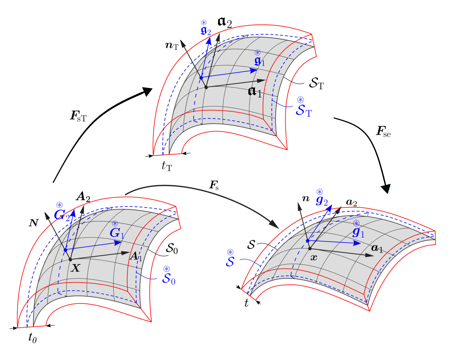
The parametric description of the mid-surface in the reference and the current configuration can be written as (see Fig. 2)

Refer to caption
Figure 2: Multiplicative deformation decomposition of layered surface continua. $\mathcal{S}_{0}$, $\mathcal{S}_{\text{T}}$ and $\mathcal{S}$ denote the mid-surface in reference, intermediate and current configuration and their corresponding tangent vectors are $\boldsymbol{A}_{i}$, $\boldsymbol{\mathfrak{a}}_{i}$ and $\boldsymbol{a}_{i}$. $\overset{\circledast}{\mathcal{S}}_{0}$, $\overset{\circledast}{\mathcal{S}}_{\text{T}}$ and $\overset{\circledast}{\mathcal{S}}$ are the reference, intermediate and current configuration of shell layers (through the thickness) and their corresponding tangent vectors are $\overset{\circledast}{\boldsymbol{g}}_{i}$, $\overset{\circledast}{\boldsymbol{\mathfrak{g}}}_{i}$ and $\overset{\circledast}{\boldsymbol{G}}_{i}$. $\boldsymbol{F}_{\!\text{s}}$, $\boldsymbol{F}_{\!\text{sT}}$ and $\boldsymbol{F}_{\!\text{se}}$ are total, thermal and elastic surface deformation gradients.
$$\begin{array}[]{lllll}\boldsymbol{X}_{\!\text{s}}\!\!\!&=&\!\!\!\displaystyle\boldsymbol{X}_{\!\text{s}}(\xi^{\alpha})~{},\quad\boldsymbol{x}_{\text{s}}\!\!\!&=&\!\!\!\displaystyle\boldsymbol{x}_{\text{s}}(\xi^{\alpha},t)~{},\end{array}$$ (119)

where $\xi^{\alpha}$ are convective coordinates and the corresponding tangent vectors are

$$\begin{array}[]{lllll}\boldsymbol{A}_{\alpha}\!\!\!&=&\!\!\!\displaystyle\frac{\partial{\boldsymbol{X}_{\!\text{s}}}}{\partial{\xi^{\alpha}}}~{},\quad\boldsymbol{a}_{\alpha}\!\!\!&=&\!\!\!\displaystyle\frac{\partial{\boldsymbol{x}_{\text{s}}}}{\partial{\xi^{\alpha}}}~{}.\end{array}$$ (120)

Next, the co-variant metric is obtained by the inner product, i.e.

$$\begin{array}[]{lllll}A_{\alpha\beta}\!\!\!&=&\!\!\!\boldsymbol{A}_{\alpha}\cdot\boldsymbol{A}_{\beta}~{},\quad a_{\alpha\beta}\!\!\!&=&\!\!\!\boldsymbol{a}_{\alpha}\cdot\boldsymbol{a}_{\beta}~{}.\end{array}$$ (121)

The contra-variant metric is the inverse of the co-variant metric, i.e.

$$\begin{array}[]{lllll}[A^{\alpha\beta}]\!\!\!&=&\!\!\![A_{\alpha\beta}]^{-1}~{},\quad[a^{\alpha\beta}]\!\!\!&=&\!\!\![a_{\alpha\beta}]^{-1}~{}.\end{array}$$ (122)

The dual tangent vectors can then be defined as

$$\begin{array}[]{lllll}\boldsymbol{A}^{\alpha}\!\!\!&:=&\!\!\!A^{\alpha\beta}\,\boldsymbol{A}_{\beta}~{},\quad\boldsymbol{a}^{\alpha}\!\!\!&:=&\!\!\!a^{\alpha\beta}\,\boldsymbol{a}_{\beta}~{}.\end{array}$$ (123)

The unit normal vector of the surface in its reference and current configuration can then be written as

$$\begin{array}[]{lllll}\boldsymbol{N}\!\!\!&=&\!\!\!\displaystyle\frac{\boldsymbol{A}_{1}\times\boldsymbol{A}_{2}}{\|\boldsymbol{A}_{1}\times\boldsymbol{A}_{2}\|}~{},\quad\boldsymbol{n}\!\!\!&=&\!\!\!\displaystyle\frac{\boldsymbol{a}_{1}\times\boldsymbol{a}_{2}}{\|\boldsymbol{a}_{1}\times\boldsymbol{a}_{2}\|}~{}.\end{array}$$ (124)

The 3D identity tensor $\boldsymbol{1}$ can be written as

$$\begin{array}[]{l}\boldsymbol{1}=\boldsymbol{I}+\boldsymbol{N}\otimes\boldsymbol{N}=\boldsymbol{i}+\boldsymbol{n}\otimes\boldsymbol{n}~{},\end{array}$$ (125)

where $\boldsymbol{I}$ and $\boldsymbol{i}$ are the surface identity tensors in the reference and current configuration that can be written as

$$\begin{array}[]{lll}\boldsymbol{I}\!\!\!&=&\!\!\!A_{\alpha\beta}\,\boldsymbol{A}^{\alpha}\otimes\boldsymbol{A}^{\beta}=A^{\alpha\beta}\,\boldsymbol{A}_{\alpha}\otimes\boldsymbol{A}_{\beta}=\boldsymbol{A}^{\alpha}\otimes\boldsymbol{A}_{\alpha}=\boldsymbol{A}_{\alpha}\otimes\boldsymbol{A}^{\alpha}~{},\end{array}$$ (126)
$$\begin{array}[]{lll}\boldsymbol{i}\!\!\!&=&\!\!\!a_{\alpha\beta}\,\boldsymbol{a}^{\alpha}\otimes\boldsymbol{a}^{\beta}=a^{\alpha\beta}\,\boldsymbol{a}_{\alpha}\otimes\boldsymbol{a}_{\beta}=\boldsymbol{a}^{\alpha}\otimes\boldsymbol{a}_{\alpha}=\boldsymbol{a}_{\alpha}\otimes\boldsymbol{a}^{\alpha}~{}.\end{array}$$ (127)

The surface gradient operator for a general scalar, surface vector and surface tensor131313Surface vectors and tensors have only in-plane components. in the reference and current configuration are

$$\begin{array}[]{lll}\displaystyle\text{Grad}_{\text{s}}\,\Phi\!\!\!&:=&\!\!\!\displaystyle\Phi_{,\alpha}\,\boldsymbol{A}^{\alpha}~{},\\[8.53581pt] \displaystyle\text{Grad}_{\text{s}}\,\boldsymbol{u}_{\text{s}}\!\!\!&:=&\!\!\!\displaystyle\boldsymbol{u}_{\text{s}\,,\beta}\otimes\boldsymbol{A}^{\beta}=u^{\alpha}_{;;\beta}\,\boldsymbol{A}_{\alpha}\otimes\boldsymbol{A}^{\beta}~{},\\[8.53581pt] \displaystyle\text{Grad}_{\text{s}}\,\boldsymbol{U}_{\!\text{s}}\!\!\!&:=&\!\!\!\displaystyle\boldsymbol{U}_{\!\text{s}\,,\gamma}\otimes\boldsymbol{A}^{\gamma}=U^{\alpha\beta}_{~{}~{};;\gamma}\,\boldsymbol{A}_{\alpha}\otimes\boldsymbol{A}_{\beta}\otimes\boldsymbol{A}^{\gamma}{}\\ \end{array}$$ (128)

and

$$\begin{array}[]{lll}\displaystyle\text{grad}_{\text{s}}\,\Phi\!\!\!&:=&\!\!\!\displaystyle\Phi_{,\alpha}\,\boldsymbol{a}^{\alpha}~{},\\[8.53581pt] \displaystyle\text{grad}_{\text{s}}\,\boldsymbol{v}_{\text{s}}\!\!\!&:=&\!\!\!\displaystyle\boldsymbol{v}_{\!\text{s}\,,\beta}\otimes\boldsymbol{a}^{\beta}=v^{\alpha}_{~{};\beta}\,\boldsymbol{a}_{\alpha}\otimes\boldsymbol{a}^{\beta}~{},\\[8.53581pt] \displaystyle\text{grad}_{\text{s}}\,\boldsymbol{V}_{\!\text{s}}\!\!\!&:=&\!\!\!\displaystyle\boldsymbol{V}_{\!\text{s}\,,\gamma}\otimes\boldsymbol{a}^{\gamma}=V^{\alpha\beta}_{~{}~{}~{};\gamma}\,\boldsymbol{a}_{\alpha}\otimes\boldsymbol{a}_{\beta}\otimes\boldsymbol{a}^{\gamma}~{},\\ \end{array}$$ (129)

where “;;” and “;” are the co-variant derivatives in the reference and current configuration. They are defined as [97]

$$\begin{array}[]{lll}u^{\alpha}_{;;\beta}\!\!\!&:=&\!\!\!u^{\alpha}_{,\beta}+u^{\gamma}\,\Gamma_{\text{s}0\,\gamma\beta}^{\alpha}~{},\\[8.53581pt] \displaystyle U^{\alpha\beta}_{~{}~{};;\gamma}\!\!\!&:=&\!\!\!\displaystyle U^{\alpha\beta}_{~{}~{},\gamma}+U^{\delta\beta}\,\Gamma_{\text{s}0\,\delta\gamma}^{\alpha}+U^{\alpha\delta}\,\Gamma_{\text{s}0\,\delta\gamma}^{\beta}~{},\\[8.53581pt] v^{\alpha}_{;\beta}\!\!\!&:=&\!\!\!v^{\alpha}_{,\beta}+v^{\gamma}\,\Gamma_{\text{s}\,\gamma\beta}^{\alpha}~{},\\[8.53581pt] V^{\alpha\beta}_{~{}~{}~{};\gamma}\!\!\!&:=&\!\!\!V^{\alpha\beta}_{~{}~{}~{},\gamma}+V^{\delta\beta}\,\Gamma_{\text{s}\,\delta\gamma}^{\alpha}+V^{\alpha\delta}\,\Gamma_{\text{s}\,\delta\gamma}^{\beta}~{},\end{array}$$ (130)

where the surface Christoffel symbols, $\Gamma_{\text{s}0\,\alpha\beta}^{\gamma}$ and $\Gamma_{\text{s}\,\alpha\beta}^{\gamma}$, are defined as

$$\begin{array}[]{lllll}\Gamma_{\text{s}0\,\alpha\beta}^{\gamma}\!\!\!&:=&\!\!\!\boldsymbol{A}_{\alpha,\beta}\cdot\boldsymbol{A}^{\gamma}~{},\quad\Gamma_{\text{s}\,\alpha\beta}^{\gamma}\!\!\!&:=&\!\!\!\boldsymbol{a}_{\alpha,\beta}\cdot\boldsymbol{a}^{\gamma}~{}.\end{array}$$ (131)

The co-variant derivative of the surface tangent and dual tangent vector are defined as [97]

$$\begin{array}[]{llllll}\boldsymbol{A}_{\alpha;;\beta}\!\!\!&:=&\!\!\!\boldsymbol{A}_{\alpha,\beta}-\boldsymbol{A}_{\gamma}\,\Gamma_{\text{s}0\,\alpha\beta}^{\gamma}~{},&\boldsymbol{A}^{\alpha}_{;;\beta}\!\!\!&:=&\!\!\!\boldsymbol{A}^{\alpha}_{,\beta}+\boldsymbol{A}^{\gamma}\,\Gamma_{\text{s}0\,\gamma\beta}^{\alpha}~{},\\[8.53581pt] \boldsymbol{a}_{\alpha;\beta}\!\!\!&:=&\!\!\!\boldsymbol{a}_{\alpha,\beta}-\boldsymbol{a}_{\gamma}\,\Gamma_{\text{s}\,\alpha\beta}^{\gamma}~{},&\boldsymbol{a}^{\alpha}_{;\beta}\!\!\!&:=&\!\!\!\boldsymbol{a}^{\alpha}_{,\beta}+\boldsymbol{a}^{\gamma}\,\Gamma_{\text{s}\,\gamma\beta}^{\alpha}~{}.\end{array}$$ (132)

Similar to the 3D case, see Eqs. (31) and (32), the co-variant derivative of the metric tensor in the reference and current configuration are zero, i.e. [64]

$$\begin{array}[]{l}A_{\alpha\beta;;\gamma}=0~{},\quad A^{\alpha\beta}_{~{}~{};;\gamma}=0~{},\quad a_{\alpha\beta;\gamma}=0~{},\quad a^{\alpha\beta}_{~{}~{};\gamma}=0~{},\end{array}$$ (133)

so that the contra-variant derivatives follow as

$$\begin{array}[]{lllll}U_{\alpha\beta;;}^{~{}~{}~{}\gamma}\!\!\!&=&\!\!\!A_{\alpha\delta}\,A_{\beta\xi}\,A^{\gamma\eta}\,U^{\delta\xi}_{~{}~{};;\eta}~{},\quad V_{\alpha\beta;}^{~{}~{}\gamma}\!\!\!&=&\!\!\!a_{\alpha\delta}\,a_{\beta\xi}\,a^{\gamma\eta}\,V^{\delta\xi}_{~{}~{};\eta}~{}.\end{array}$$ (134)

Furthermore, the surface divergence of a surface vector and a surface second order tensor is defined as

$$\begin{array}[]{lllllllllll}\text{Div}_{\text{s}}\,\boldsymbol{u}_{\text{s}}\!\!\!&:=&\!\!\!u^{\alpha}_{;;\alpha}~{},&\text{div}_{\text{s}}\,\boldsymbol{v}_{\text{s}}\!\!\!&:=&\!\!\!v^{\alpha}_{;\alpha}~{},\quad\text{Div}_{\text{s}}\,\boldsymbol{U}_{\!\text{s}}\!\!\!&:=&\!\!\!U^{\alpha\beta}_{~{}~{};;\beta}\,\boldsymbol{a}_{\alpha}~{},&\text{div}_{\text{s}}\,\boldsymbol{V}_{\!\text{s}}\!\!\!&:=&\!\!\!V^{\alpha\beta}_{~{}~{};\beta}\,\boldsymbol{a}_{\alpha}~{}.\\[8.53581pt] \end{array}$$ (135)

Using Ricci’s theorem (Eqs. (31) and (32)), it can be shown that

$$\begin{array}[]{lllll}\boldsymbol{A}_{\alpha\|\beta}\!\!\!&=&\!\!\!\boldsymbol{A}_{\alpha;;\beta}-\boldsymbol{N}\,\Gamma^{3}_{0~{}\alpha\beta}=0~{},\quad\boldsymbol{a}_{\alpha|\beta}\!\!\!&=&\!\!\!\boldsymbol{a}_{\alpha;\beta}-\boldsymbol{n}\,\Gamma^{3}_{\alpha\beta}=0~{},\end{array}$$ (136)

where the co-variant components of the curvature tensor are defined by

$$\begin{array}[]{lllll}b_{0\,\alpha\beta}\!\!\!&:=&\!\!\!\Gamma^{3}_{0~{}\alpha\beta}:=\boldsymbol{N}\cdot\boldsymbol{A}_{\alpha,\beta}=\boldsymbol{N}\cdot\boldsymbol{A}_{\alpha;;\beta}~{},\quad b_{\alpha\beta}\!\!\!&:=&\!\!\!\Gamma^{3}_{\alpha\beta}:=\boldsymbol{n}\cdot\boldsymbol{a}_{\alpha,\beta}=\boldsymbol{n}\cdot\boldsymbol{a}_{\alpha;\beta}~{},\end{array}$$ (137)

and Gauss’ formula can be written as

$$\begin{array}[]{lllll}\boldsymbol{A}_{\alpha;;\beta}\!\!\!&=&\!\!\!b_{0\,\alpha\beta}\,\boldsymbol{N}~{},\quad\boldsymbol{a}_{\alpha;\beta}\!\!\!&=&\!\!\!b_{\alpha\beta}\,\boldsymbol{n}~{}.\end{array}$$ (138)

Using differentiation of $\boldsymbol{N}\cdot\boldsymbol{A}_{\alpha}=0$, $\boldsymbol{N}\cdot\boldsymbol{N}=1$ and their counterparts in the current configuration, it can be shown that

$$\begin{array}[]{lllllllll}\Gamma^{3}_{0\,3\beta}\!\!\!&=&\!\!\!0~{},\quad\Gamma^{3}_{3\beta}\!\!\!&=&\!\!\!0~{},\quad\Gamma^{\beta}_{0\,3\alpha}\!\!\!&=&\!\!\!-b^{\beta}_{0~{}\alpha}~{},\quad\Gamma^{\beta}_{3\alpha}\!\!\!&=&\!\!\!-b^{\beta}_{\alpha}~{}.\end{array}$$ (139)

Using these relations, Weingarten’s formula can be obtained as

$$\begin{array}[]{lllll}\boldsymbol{N}_{\!,\alpha}\!\!\!&=&\!\!\!-b^{\beta}_{0\,\alpha}\,\boldsymbol{A}_{\beta}~{},\quad\boldsymbol{n}_{,\alpha}\!\!\!&=&\!\!\!-b^{\beta}_{\alpha}\,\boldsymbol{a}_{\beta}~{},\end{array}$$ (140)

or based on the gradient operator as

$$\begin{array}[]{lllll}\displaystyle-\text{Grad}_{\text{s}}\,\boldsymbol{N}=b_{0\,\alpha\beta}\,\boldsymbol{A}^{\alpha}\otimes\boldsymbol{A}^{\beta}\!\!\!&:=&\!\!\!\boldsymbol{b}_{0}~{},\quad\displaystyle-\text{grad}_{\text{s}}\,\boldsymbol{n}=b_{\alpha\beta}\,\boldsymbol{a}^{\alpha}\otimes\boldsymbol{a}^{\beta}\!\!\!&:=&\!\!\!\boldsymbol{b}~{},\end{array}$$ (141)

which allows us to identify the curvature tensors as the surface gradient of the surface normals. The contra-variant components of $\boldsymbol{b}_{0}$ and $\boldsymbol{b}$ can be obtained as

$$\begin{array}[]{lllll}b^{\alpha\beta}_{0}\!\!\!&=&\!\!\!A^{\alpha\gamma}\,b_{0\,\gamma\delta}\,A^{\delta\beta}~{},\quad b^{\alpha\beta}\!\!\!&=&\!\!\!a^{\alpha\gamma}\,b_{\gamma\delta}\,a^{\delta\beta}~{}.\end{array}$$ (142)

The mean and Gaussian curvatures $H_{0}$ and $\kappa_{0}$ ($H$ and $\kappa$) of the reference (current) configuration are defined as

$$\begin{array}[]{l}H_{0}:=\displaystyle\frac{1}{2}\boldsymbol{b}_{0}:\boldsymbol{I}=\frac{1}{2}b^{\alpha}_{0\,\alpha}~{},~{}H:=\displaystyle\frac{1}{2}\boldsymbol{b}:\boldsymbol{i}=\frac{1}{2}b^{\alpha}_{\alpha}~{},\end{array}$$ (143)
$$\begin{array}[]{l}\kappa_{0}:=\displaystyle\det(\boldsymbol{b}_{0})=\frac{\det[b_{0\,\alpha\beta}]}{\det[A_{\gamma\delta}]}~{},~{}\kappa:=\displaystyle\det(\boldsymbol{b})=\frac{\det[b_{\alpha\beta}]}{\det[a_{\gamma\delta}]}~{},\end{array}$$ (144)

where the surface determinant for a general surface tensor $\boldsymbol{T}_{\text{s}}=T_{\alpha\beta}\,\boldsymbol{l}^{\alpha}\otimes\boldsymbol{k}^{\beta}$ is defined as141414$\boldsymbol{l}^{\alpha}$ and $\boldsymbol{k}^{\beta}$ are general base vectors, e.g. $\boldsymbol{a}^{\alpha}$ and $\boldsymbol{A}^{\alpha}$.

$$\begin{array}[]{lll}\displaystyle\text{det}_{\text{s}}\,\boldsymbol{T}_{\text{s}}\!\!\!&:=&\!\!\!\displaystyle\frac{[(\boldsymbol{T}_{\text{s}}\cdot\boldsymbol{y}_{1})\times(\boldsymbol{T}_{\text{s}}\cdot\boldsymbol{y}_{2})]\cdot\boldsymbol{y}_{4}}{[\boldsymbol{y}_{1}\times\boldsymbol{y}_{2}]\cdot\boldsymbol{y}_{3}}~{},\end{array}$$ (145)

where $\boldsymbol{y}_{1}$ and $\boldsymbol{y}_{2}$ lie in the surface spanned by $\boldsymbol{k}^{\beta}$, i.e. they do not have any out of plane components and are not parallel to each other, and $\boldsymbol{y}_{3}$ is the unit normal vector to the surface. $\boldsymbol{y}_{4}$ is the unit normal vector to the plane spanned by $\boldsymbol{l}^{\alpha}$. A similar definition of the determinant of surface tensors can be found in Javili et al. [104]. Alternative to Eq. (143), the mean and Gaussian curvatures can be defined from the principal curvatures $\kappa_{\alpha}$ as

$$\begin{array}[]{l}H_{0}=\displaystyle\frac{1}{2}(\kappa_{0\,1}+\kappa_{0\,2})~{},~{}H=\displaystyle\frac{1}{2}(\kappa_{1}+\kappa_{2})~{},\end{array}$$ (146)
$$\begin{array}[]{l}\kappa_{0}=\displaystyle\kappa_{0\,1}\,\kappa_{0\,2}~{},~{}\kappa=\displaystyle\kappa_{1}\,\kappa_{2}~{},\end{array}$$ (147)

where $\kappa_{0\,\alpha}$ and $\kappa_{\alpha}$ are the eigenvalues of matrix $[b_{0\,\alpha\beta}\,A^{\beta\gamma}]$ and $[b_{\alpha\beta}\,a^{\beta\gamma}]$, respectively.
Assuming Kirchhoff-Love kinematics, the position of a point on the shell layers $\accentset{\circledast}{\mathcal{S}}_{0}$ and $\accentset{\circledast}{\mathcal{S}}$ can be written as

$$\begin{array}[]{lllll}\accentset{\circledast}{\boldsymbol{X}}\!\!\!&:=&\!\!\!\boldsymbol{X}_{\!\text{s}}+\xi\,\boldsymbol{N}~{},\quad\accentset{\circledast}{\boldsymbol{x}}\!\!\!&:=&\!\!\!\boldsymbol{x}_{\text{s}}+\xi\,\lambda_{3}\,\boldsymbol{n}~{},\end{array}$$ (148)

where $\xi$ is the thickness coordinate and $\lambda_{3}$ is the stretch in the direction of the surface normal. The tangent vectors of $\accentset{\circledast}{\boldsymbol{X}}$ and $\accentset{\circledast}{\boldsymbol{x}}$ follow as

$$\begin{array}[]{lll}\displaystyle\accentset{\circledast}{\boldsymbol{G}}_{\alpha}\!\!\!&:=&\!\!\!\displaystyle\frac{\partial{\accentset{\circledast}{\boldsymbol{X}}}}{\partial{\xi^{\alpha}}}=\boldsymbol{A}_{\alpha}-\xi\,b_{0\,\alpha}^{\gamma}\,\boldsymbol{A}_{\gamma}=\boldsymbol{A}_{\alpha}-\xi\,b_{0\,\alpha\gamma}\,\boldsymbol{A}^{\gamma}~{},\end{array}$$ (149)
$$\begin{array}[]{lll}\displaystyle\accentset{\circledast}{\boldsymbol{g}}_{\alpha}\!\!\!&:=&\!\!\!\displaystyle\frac{\partial{\accentset{\circledast}{\boldsymbol{x}}}}{\partial{\xi^{\alpha}}}=\boldsymbol{a}_{\alpha}-\xi\,b_{\alpha}^{\gamma}\,\boldsymbol{a}_{\gamma}=\boldsymbol{a}_{\alpha}-\xi\,\lambda_{3}\,b_{\alpha\gamma}\,\boldsymbol{a}^{\gamma}~{},\end{array}$$ (150)

and their corresponding metric up to leading order in $\xi$ are151515Assuming $\lambda_{3}\simeq 1$.

$$\begin{array}[]{lllll}\accentset{\circledast}{\boldsymbol{G}}_{\alpha\beta}\!\!\!&:=&\!\!\!\accentset{\circledast}{\boldsymbol{G}}_{\alpha}\cdot\accentset{\circledast}{\boldsymbol{G}}_{\beta}\simeq A_{\alpha\beta}-2\xi\,b_{0\,\alpha\beta}~{},\quad\accentset{\circledast}{\boldsymbol{g}}_{\alpha\beta}\!\!\!&:=&\!\!\!\accentset{\circledast}{\boldsymbol{g}}_{\alpha}\cdot\accentset{\circledast}{\boldsymbol{g}}_{\beta}\simeq a_{\alpha\beta}-2\xi\,b_{\alpha\beta}~{}.\end{array}$$ (151)

4.2 Kinematics of surface deformation

The deformation gradient of layer $\accentset{\circledast}{\mathcal{S}}$ follows from Eq. (38) as

$$\begin{array}[]{lll}\accentset{\circledast}{\boldsymbol{F}}\!\!\!&=&\!\!\!\displaystyle\frac{\partial{\accentset{\circledast}{\boldsymbol{x}}}}{\partial{\accentset{\circledast}{\boldsymbol{X}}}}=\accentset{\ast}{\boldsymbol{F}}+\lambda_{3}\,\boldsymbol{n}\otimes\boldsymbol{N}~{},\end{array}$$ (152)

and it transforms $\mathrm{d}\accentset{\circledast}{\boldsymbol{X}}$ to $\mathrm{d}\accentset{\circledast}{\boldsymbol{x}}$ as

$$\begin{array}[]{lll}\mathrm{d}\accentset{\circledast}{\boldsymbol{x}}\!\!\!&=&\!\!\!\displaystyle\accentset{\circledast}{\boldsymbol{F}}\,\mathrm{d}\accentset{\circledast}{\boldsymbol{X}}~{}.\end{array}$$ (153)

The in-plane part of $\accentset{\circledast}{\boldsymbol{F}}$, $\accentset{\ast}{\boldsymbol{F}}$, can be written based on the tangent vectors as

$$\begin{array}[]{lll}\accentset{\ast}{\boldsymbol{F}}\!\!\!&=&\!\!\!\displaystyle\frac{\partial{\accentset{\circledast}{\boldsymbol{x}}}}{\partial{\xi^{\alpha}}}\otimes\frac{\partial{\xi^{\alpha}}}{\partial{\accentset{\circledast}{\boldsymbol{X}}}}=\accentset{\circledast}{\boldsymbol{g}}_{\alpha}\otimes~{}\accentset{\circledast}{\boldsymbol{G}}^{\alpha}~{},\end{array}$$ (154)

and it transforms $\accentset{\circledast}{\boldsymbol{G}}_{\alpha}$ as

$$\begin{array}[]{lll}\accentset{\circledast}{\boldsymbol{g}}_{\alpha}\!\!\!&=&\!\!\!\displaystyle\accentset{\circledast}{\boldsymbol{F}}\,\accentset{\circledast}{\boldsymbol{G}}_{\alpha}=\accentset{\ast}{\boldsymbol{F}}\,\accentset{\circledast}{\boldsymbol{G}}_{\alpha}~{}.\end{array}$$ (155)

The mid-surface deformation gradient (i.e. for layer $\mathcal{S}$) is defined as

$$\begin{array}[]{lll}\displaystyle\accentset{0}{\boldsymbol{F}}\!\!\!&:=&\!\!\!\displaystyle\accentset{\circledast}{\boldsymbol{F}}(\xi=0)=\boldsymbol{F}_{\!\text{s}}+\lambda_{3}\,\boldsymbol{n}\otimes\boldsymbol{N}~{},\end{array}$$ (156)

where $\boldsymbol{F}_{\!\text{s}}=\accentset{\ast}{\boldsymbol{F}}(\xi=0)$ is the in-plane deformation gradient of the mid-surface, i.e.

$$\begin{array}[]{lll}\boldsymbol{F}_{\!\text{s}}\!\!\!&=&\!\!\!\boldsymbol{a}_{\alpha}\otimes\boldsymbol{A}^{\alpha}~{}.\end{array}$$ (157)

The deformation gradient $\accentset{\circledast}{\boldsymbol{F}}$ can be decomposed into thermal and elastic parts $\accentset{\circledast}{\boldsymbol{F}}_{\!\text{T}}$ and $\accentset{\circledast}{\boldsymbol{F}}_{\!\text{e}}$ as

$$\begin{array}[]{lll}\displaystyle\accentset{\circledast}{\boldsymbol{F}}\!\!\!&=&\!\!\!\displaystyle\accentset{\circledast}{\boldsymbol{F}}_{\!\text{e}}\,\accentset{\circledast}{\boldsymbol{F}}_{\!\text{T}}~{}.\end{array}$$ (158)

$\accentset{\circledast}{\boldsymbol{F}}_{\!\text{T}}$ pushes forward $\mathrm{d}\accentset{\circledast}{\boldsymbol{X}}$ to the intermediate configuration as

$$\begin{array}[]{lll}\mathrm{d}\accentset{\circledast}{\boldsymbol{\mathfrak{X}}}\!\!\!&=&\!\!\!\accentset{\circledast}{\boldsymbol{F}}_{\!\text{T}}\,\mathrm{d}\accentset{\circledast}{\boldsymbol{X}}~{}.\end{array}$$ (159)

The tangent vectors in the intermediate configuration $\accentset{\circledast}{\boldsymbol{\mathfrak{g}}}_{\alpha}$ are

$$\begin{array}[]{lll}\accentset{\circledast}{\boldsymbol{\mathfrak{g}}}_{\alpha}\!\!\!&=&\!\!\!\accentset{\circledast}{\boldsymbol{\mathfrak{X}}}_{,\alpha}~{}.\end{array}$$ (160)

$\accentset{\circledast}{\boldsymbol{F}}_{\!\text{e}}$ and $\accentset{\circledast}{\boldsymbol{F}}_{\!\text{T}}$ are

$$\begin{array}[]{lll}\accentset{\circledast}{\boldsymbol{F}}_{\!\text{e}}\!\!\!&=&\!\!\!\accentset{\ast}{\boldsymbol{F}}_{\!\text{e}}+\lambda_{\text{e}\,3}\,\boldsymbol{n}\otimes\boldsymbol{n}_{\text{T}}~{},\end{array}$$ (161)
$$\begin{array}[]{lll}\accentset{\circledast}{\boldsymbol{F}}_{\!\text{T}}\!\!\!&=&\!\!\!\accentset{\ast}{\boldsymbol{F}}_{\!\text{T}}+\lambda_{\text{T}\,3}\,\boldsymbol{n}_{\text{T}}\otimes\boldsymbol{N}~{},\end{array}$$ (162)

where $\lambda_{\text{e}\,3}$ and $\lambda_{\text{T}\,3}$ are the elastic and thermal parts of the stretch in the thickness direction, and $\boldsymbol{n}_{\text{T}}$ is the unit normal vector of the surface in the intermediate configuration. The surface right Cauchy-Green deformation tensor $\accentset{\circledast}{\boldsymbol{C}}$ and its thermal and elastic part $\accentset{\circledast}{\boldsymbol{C}}_{\!\text{T}}$ and $\accentset{\circledast}{\boldsymbol{C}}_{\!\text{e}}$ are

$$\begin{array}[]{lll}\accentset{\circledast}{\boldsymbol{C}}\!\!\!&=&\!\!\!\accentset{\circledast}{\boldsymbol{F}}^{\text{T}}\,\accentset{\circledast}{\boldsymbol{F}}=\accentset{\circledast}{\boldsymbol{F}}_{\!\text{T}}^{\text{T}}\,\accentset{\circledast}{\boldsymbol{C}}_{\!\text{e}}\,\accentset{\circledast}{\boldsymbol{F}}_{\!\text{T}}~{},\\[8.53581pt] \accentset{\circledast}{\boldsymbol{C}}_{\!\text{T}}\!\!\!&=&\!\!\!\accentset{\circledast}{\boldsymbol{F}}_{\!\text{T}}^{\text{T}}\,\accentset{\circledast}{\boldsymbol{F}}_{\!\text{T}}=\accentset{\ast}{\boldsymbol{C}}_{\!\text{T}}+\lambda_{\text{T}\,3}^{2}\,\boldsymbol{N}\otimes\boldsymbol{N}~{},\\[8.53581pt] \accentset{\circledast}{\boldsymbol{C}}_{\!\text{e}}\!\!\!&=&\!\!\!\accentset{\circledast}{\boldsymbol{F}}_{\!\text{e}}^{\text{T}}\,\accentset{\circledast}{\boldsymbol{F}}_{\!\text{e}}=\accentset{\ast}{\boldsymbol{C}}_{\!\text{e}}+\lambda_{\text{e}\,3}^{2}\,\boldsymbol{n}_{\text{T}}\otimes\boldsymbol{n}_{\text{T}}~{},\end{array}$$ (163)

where $\accentset{\circledast}{\boldsymbol{C}}_{\!\text{T}}$ and $\accentset{\circledast}{\boldsymbol{C}}_{\!\text{e}}$ are

$$\begin{array}[]{lll}\accentset{\ast}{\boldsymbol{C}}_{\!\text{T}}\!\!\!&=&\!\!\!\accentset{\ast}{\boldsymbol{F}}_{\!\text{T}}^{\text{T}}\,\accentset{\ast}{\boldsymbol{F}}_{\!\text{T}}=\accentset{\circledast}{\mathfrak{g}}_{\alpha\beta}\accentset{\circledast}{\boldsymbol{G}}^{\alpha}\otimes\accentset{\circledast}{\boldsymbol{G}}^{\beta}~{},\end{array}$$ (164)
$$\begin{array}[]{lll}\accentset{\ast}{\boldsymbol{C}}_{\!\text{e}}\!\!\!&=&\!\!\!\accentset{\ast}{\boldsymbol{F}}_{\!\text{e}}^{\text{T}}\,\accentset{\ast}{\boldsymbol{F}}_{\!\text{e}}=\accentset{\circledast}{g}_{\alpha\beta}\,\accentset{\circledast}{\boldsymbol{\mathfrak{g}}}^{\alpha}\otimes\accentset{\circledast}{\boldsymbol{\mathfrak{g}}}^{\beta}~{},\end{array}$$ (165)

with $\accentset{\circledast}{\mathfrak{g}}_{\alpha\beta}=\accentset{\circledast}{\boldsymbol{\mathfrak{g}}}_{\alpha}\cdot\accentset{\circledast}{\boldsymbol{\mathfrak{g}}}_{\beta}$. The velocity gradient $\accentset{\circledast}{\boldsymbol{l}}$ can be written as

$$\begin{array}[]{lll}\displaystyle\accentset{\circledast}{\boldsymbol{l}}\!\!\!&:=&\!\!\!\displaystyle\dot{\accentset{\circledast}{\boldsymbol{F}}}\,\accentset{\circledast}{\boldsymbol{F}}^{-1}=\dot{\accentset{\circledast}{g}}_{\alpha}\otimes\accentset{\circledast}{\boldsymbol{g}}^{\alpha}+\dot{\boldsymbol{n}}\otimes\boldsymbol{n}+\frac{\dot{\lambda}_{3}}{\lambda_{3}}\,\boldsymbol{n}\otimes\boldsymbol{n}~{}.\end{array}$$ (166)

The velocity gradient of the mid-surface is $\accentset{0}{\boldsymbol{l}}=\accentset{\circledast}{\boldsymbol{l}}(\xi=0)$. For the mid-surface in the intermediate configuration, the tangent vectors can be written as161616$\boldsymbol{F}_{\!\text{sT}}$ and $\boldsymbol{F}_{\!\text{se}}$ are such that $\boldsymbol{F}_{\!\text{s}}=\boldsymbol{F}_{\!\text{se}}\,\boldsymbol{F}_{\!\text{sT}}$.

$$\begin{array}[]{lll}\boldsymbol{\mathfrak{a}}_{\alpha}\!\!\!&=&\!\!\!\boldsymbol{F}_{\!\text{sT}}\,\boldsymbol{A}_{\alpha}~{},\end{array}$$ (167)

and the curvature tensor as

$$\begin{array}[]{lll}\boldsymbol{\mathfrak{b}}\!\!\!&=&\!\!\!-\text{grad}_{\text{T}}\,\boldsymbol{n}_{\text{T}}=\mathfrak{b}_{\alpha\beta}\,\boldsymbol{\mathfrak{a}}^{\alpha}\otimes\boldsymbol{\mathfrak{a}}^{\beta}~{},\end{array}$$ (168)

where $\mathfrak{b}_{\alpha\beta}$ is

$$\begin{array}[]{lllll}\mathfrak{b}_{\alpha\beta}\!\!\!&=&\!\!\!\boldsymbol{\mathfrak{a}}_{\alpha,\beta}\cdot\boldsymbol{n}_{\text{T}}~{}\quad\text{with}\quad\boldsymbol{\mathfrak{a}}_{\alpha,\beta}\!\!\!&=&\!\!\!\boldsymbol{F}_{\!\text{sT},\beta}\,\boldsymbol{A}_{\alpha}+\boldsymbol{F}_{\!\text{sT}}\,\boldsymbol{A}_{\alpha,\beta}~{}.\end{array}$$ (169)

The curvature change relative to the intermediate configuration is

$$\begin{array}[]{lll}\boldsymbol{\kappa}\!\!\!&=&\!\!\!\boldsymbol{b}^{\flat\lhd}-\boldsymbol{\mathfrak{b}}^{\flat\lhd(\boldsymbol{F}_{\text{T}})}=k_{\alpha\beta}\,\boldsymbol{A}^{\alpha}\otimes\boldsymbol{A}^{\beta}~{},\end{array}$$ (170)

with

$$\begin{array}[]{lllllll}\kappa_{\alpha\beta}\!\!\!&=&\!\!\!b_{\alpha\beta}-\mathfrak{b}_{\alpha\beta}~{},\quad\boldsymbol{b}^{\flat\lhd}\!\!\!&=&\!\!\!\boldsymbol{F}_{\!\text{s}}^{\text{T}}\,\boldsymbol{b}\,\boldsymbol{F}_{\!\text{s}}~{},\quad\boldsymbol{\mathfrak{b}}^{\flat\lhd(\boldsymbol{F}_{\text{T}})}\!\!\!&=&\!\!\!\boldsymbol{F}_{\!\text{sT}}^{\text{T}}\,\boldsymbol{\mathfrak{b}}\,\boldsymbol{F}_{\!\text{sT}}~{}.\end{array}$$ (171)

The local area change between the reference and current configuration can is given by

$$\begin{array}[]{lll}J_{\text{s}}\!\!\!&:=&\!\!\!\displaystyle\frac{\partial{a}}{\partial{A}}=\text{det}_{\text{s}}\,\boldsymbol{F}_{\!\text{s}}~{}.\end{array}$$ (172)

4.3 Surface stress and moment tensors

The Cauchy stress tensor of the Kirchhoff-Love shell formulation, $\mbox{\boldmath$\sigma$}_{\text{KL}}$, and the 3D Stress tensor $\sigma$ can be connected by replacing $\sigma$ by $\mbox{\boldmath$\sigma$}_{\text{KL}}/t$, where $t$ is the current thickness of the shell171717$\lambda_{3,i}$ is neglected in the current work (for example see Eq. (151)). The contribution of this term is included in Cirak and Ortiz [56]. Furthermore, for Kirchhoff-Love shells, $\sigma^{33}=\sigma^{3\alpha}=0$. $\mbox{\boldmath$\sigma$}_{\text{KL}}$ can be obtained from $\sigma$ such that the energy of 3D and surface continua is equal, see Roohbakhshan and Sauer [35].. $\mbox{\boldmath$\sigma$}_{\text{KL}}$ (force per length) can be written as

$$\begin{array}[]{lll}\mbox{\boldmath$\sigma$}_{\text{KL}}\!\!\!&=&\!\!\!N^{\alpha\beta}\,\boldsymbol{a}_{\alpha}\otimes\boldsymbol{a}_{\beta}+S^{\alpha}\,\boldsymbol{a}_{\alpha}\otimes\boldsymbol{n}~{},\end{array}$$ (173)

Similar to replacing $\sigma$ by $\mbox{\boldmath$\sigma$}_{\text{KL}}$, the moment vector ${\boldsymbol{m}}$ is replaced by $\boldsymbol{m}_{\text{s}}/t$. $\boldsymbol{m}_{\text{s}}$ can be written as

$$\begin{array}[]{lll}\boldsymbol{m}_{\text{s}}\!\!\!&=&\!\!\!\bar{\boldsymbol{\mu}}_{\text{s}}^{\text{T}}\,\mbox{\boldmath$\nu$}~{},\end{array}$$ (174)

where $\bar{\boldsymbol{\mu}}_{\text{s}}$ has only in-plane components and can be written as

$$\begin{array}[]{lll}\bar{\boldsymbol{\mu}}_{\text{s}}\!\!\!&=&\!\!\!\bar{\mu}^{\alpha\beta}\,\boldsymbol{a}_{\alpha}\otimes\boldsymbol{a}_{\beta}~{},\end{array}$$ (175)

so $\bar{\boldsymbol{\mu}}_{\text{s}}$ can be written based on any set of in-plane vectors that are non-parallel. It is common to write $\bar{\boldsymbol{\mu}}_{\text{s}}$ as Sauer and Duong [64]

$$\begin{array}[]{lll}\bar{\boldsymbol{\mu}}_{\text{s}}^{\text{T}}=\boldsymbol{n}\times\boldsymbol{\mu}_{\text{s}}^{\text{T}}~{},\end{array}$$ (176)

where $\boldsymbol{\mu}_{\text{s}}$ is

$$\begin{array}[]{lll}\boldsymbol{\mu}_{\text{s}}\!\!\!&=&\!\!\!-M^{\alpha\beta}\,\boldsymbol{a}_{\alpha}\otimes\boldsymbol{a}_{\beta}~{},\end{array}$$ (177)

which can be used to write $\bar{\boldsymbol{\mu}}_{\text{s}}$ as

$$\begin{array}[]{lll}\bar{\boldsymbol{\mu}}_{\text{s}}^{\text{T}}\!\!\!&=&\!\!\!M^{\alpha\beta}\,(\boldsymbol{a}_{\beta}\times\boldsymbol{n})\otimes\boldsymbol{a}_{\alpha}~{}.\end{array}$$ (178)

$\boldsymbol{a}_{\beta}\times\boldsymbol{n}$ is perpendicular to $\boldsymbol{n}$ and it can be expressed in terms of the tangent and normal vector to the boundary, $\mbox{\boldmath$\tau$}_{\!\text{v}}$ and $\nu$, as

$$\begin{array}[]{lll}\boldsymbol{a}_{\beta}\times\boldsymbol{n}\!\!\!&=&\!\!\!\tau_{\beta}\,\mbox{\boldmath$\nu$}-\nu_{\beta}\,\mbox{\boldmath$\tau$}_{\!\text{v}}~{}\quad\text{with}\quad\tau_{\beta}=\mbox{\boldmath$\tau$}_{\!\text{v}}\cdot\boldsymbol{a}_{\beta}~{};~{}\nu_{\beta}=\mbox{\boldmath$\nu$}\cdot\boldsymbol{a}_{\beta}~{},\end{array}$$ (179)

where the following relations has been used

$$\begin{array}[]{lll}\boldsymbol{a}_{\beta}=\tau_{\beta}\,\mbox{\boldmath$\tau$}_{\!\text{v}}+\nu_{\beta}\,\mbox{\boldmath$\nu$}~{},\end{array}$$ (180)
$$\begin{array}[]{l}\mbox{\boldmath$\tau$}_{\!\text{v}}\times\boldsymbol{n}=\mbox{\boldmath$\nu$}~{};~{}\mbox{\boldmath$\nu$}\times\boldsymbol{n}=-\mbox{\boldmath$\tau$}_{\!\text{v}}~{}.\end{array}$$ (181)

Using Eq. (179), it can be shown that

$$\begin{array}[]{lll}\bar{\mu}^{\alpha\beta}\,\boldsymbol{a}_{\beta}\!\!\!&=&\!\!\!M^{\alpha\beta}\,(\tau_{\beta}\,\mbox{\boldmath$\nu$}-\nu_{\beta}\,\mbox{\boldmath$\tau$}_{\!\text{v}})~{}.\end{array}$$ (182)

$\bar{\mu}^{\alpha\beta}$ can be obtained by multiplying both sides of Eq. (182) by $\boldsymbol{a}^{\gamma}$, giving

$$\begin{array}[]{lll}\bar{\mu}^{\alpha\beta}\!\!\!&=&\!\!\!M^{\alpha\gamma}\,\left(\tau_{\,\gamma}\,\nu^{\beta}-\nu_{\gamma}\,\tau^{\beta}\right)~{},\end{array}$$ (183)

where $\tau^{\beta}=\mbox{\boldmath$\tau$}_{\!\text{v}}\cdot\boldsymbol{a}^{\beta}$ and $\nu^{\beta}=\mbox{\boldmath$\nu$}\cdot\boldsymbol{a}^{\beta}$. Furthermore, $\boldsymbol{m}_{\text{s}}$ can be written in terms of $\nu$ and $\mbox{\boldmath$\tau$}_{\!\text{v}}$ as

$$\begin{array}[]{lll}\boldsymbol{m}_{\text{s}}\!\!\!&=&\!\!\!\bar{\boldsymbol{\mu}}_{\text{s}}^{\text{T}}\,\mbox{\boldmath$\nu$}=m_{\nu}\,\mbox{\boldmath$\nu$}+m_{\tau}\,\mbox{\boldmath$\tau$}_{\!\text{v}}~{},\end{array}$$ (184)

where $m_{\nu}$ and $m_{\tau}$ are

$$\begin{array}[]{lll}m_{\nu}\!\!\!&=&\!\!\!M^{\alpha\beta}\,\nu_{\alpha}\,\tau_{\beta}~{},\\ m_{\tau}\!\!\!&=&\!\!\!-M^{\alpha\beta}\,\nu_{\alpha}\,\nu_{\beta}~{}.\end{array}$$ (185)

4.4 Conservation laws for surface continua

Sahu et al. [7] and Sauer et al. [80] develop a thermomechanical Kirchhoff-Love shell formulation directly from the surface balance laws. Here on the other hand, the conservation laws for surface continua are derived as a special case of their 3D counterparts.

4.4.1 Mass balance

Using Eq. (63), ${J}=\lambda_{3}\,J_{\text{s}}$, $t=t_{0}\,\lambda_{3}$, and

$$\begin{array}[]{lll}\rho_{\text{s0}}\!\!\!&:=&\!\!\!{\rho}_{0}\,t_{0}~{},\\ \rho_{\text{s}}\!\!\!&:=&\!\!\!\displaystyle{\rho}\,t=\frac{{\rho}_{0}}{\lambda_{3}\,J_{\text{s}}}\,t_{0}\,\lambda_{3}=\frac{{\rho}_{0}}{J_{\text{s}}}\,t_{0}=\frac{\rho_{\text{s0}}}{J_{\text{s}}}~{},\end{array}$$ (186)

the mass conservation law for a surface continua can be written as

$$\begin{array}[]{lll}\rho_{\text{s0}}\!\!\!&=&\!\!\!\rho_{\text{s}}\,J_{\text{s}}~{},\end{array}$$ (187)

where $\rho_{\text{s0}}$ and $\rho_{\text{s}}$ are the surface density in the reference and current configuration.

4.4.2 Linear momentum balance

The surface linear momentum balance can be obtained directly from 3D linear momentum balance. Substituting relation $\rho_{\text{s}}:={\rho}\,t$ and replacing $\sigma$ by $\mbox{\boldmath$\sigma$}_{\text{KL}}/t$ within the 3D linear momentum balance, i.e. Eq. (66), the momentum balance for surface continua is181818The body force $\boldsymbol{f}$ is force per unit mass, so this quantity is the same for surface and volume continua, i.e. $\boldsymbol{f}_{\!\text{s}}={\boldsymbol{f}}$.

$$\begin{array}[]{lll}{\text{div}}\,\mbox{\boldmath$\sigma$}^{\text{T}}_{\text{KL}}+\rho_{\text{s}}\,\boldsymbol{f}\!\!\!&=&\!\!\!\rho_{\text{s}}\,\dot{\boldsymbol{v}}~{}.\end{array}$$ (188)

Using ${\text{div}}\,\mbox{\boldmath$\sigma$}^{\text{T}}_{\text{KL}}=\mbox{\boldmath$\sigma$}^{\text{T}}_{\text{KL},k}\cdot\boldsymbol{a}^{k}=\sigma^{ji}_{\text{KL}|j}\,\boldsymbol{a}_{i}$ and $\boldsymbol{a}_{3}=\boldsymbol{a}^{3}=\boldsymbol{n}$, ${\text{div}}\,\mbox{\boldmath$\sigma$}^{\text{T}}_{\text{KL}}$ can be written

$$\begin{array}[]{lll}\sigma^{ji}_{\text{KL}|j}\boldsymbol{a}_{i}\!\!\!&=&\!\!\!\left[\sigma^{ji}_{\text{KL},j}+\sigma^{li}_{\text{KL}}\,\Gamma^{j}_{lj}+\sigma^{jl}_{\text{KL}}\,\Gamma^{i}_{lj}\right]\boldsymbol{a}_{i}~{}.\end{array}$$ (189)

Using $\sigma^{3\alpha}_{\text{KL}}=0$, $\boldsymbol{a}_{3}\cdot\boldsymbol{a}^{\gamma}=0$, $\Gamma^{3}_{3\alpha}=0$, $\Gamma^{3}_{\alpha\beta}=b_{\alpha\beta}$ and $\Gamma^{\alpha}_{3\beta}=-b^{\alpha}_{\beta}$, Eq. (189) can be simplified as

$$\begin{array}[]{lll}{\text{div}}\,\mbox{\boldmath$\sigma$}^{\text{T}}_{\text{KL}}\!\!\!&=&\!\!\!\left[\sigma^{\beta\alpha}_{\text{KL}\,;\beta}+\sigma^{\beta 3}_{\text{KL}}\,\Gamma^{\alpha}_{3\beta}\right]\boldsymbol{a}_{\alpha}+\left[\sigma^{\beta 3}_{\text{KL}\,;\beta}+\sigma^{\alpha\beta}_{\text{KL}}\,\Gamma^{3}_{\beta\alpha}\right]\boldsymbol{a}_{3}\\[8.53581pt] \!\!\!&=&\!\!\!\left[N^{\beta\alpha}_{~{}~{};\beta}-b^{\alpha}_{\gamma}\,S^{\gamma}\right]\boldsymbol{a}_{\alpha}+\bigm{[}S^{\gamma}_{~{};\gamma}+b_{\alpha\gamma}\,N^{\alpha\gamma}\bigm{]}\boldsymbol{n}~{}.\end{array}$$ (190)

Sauer and Duong [64] obtain this relation directly from the linear momentum balance for surfaces, while it is obtained here from the corresponding 3D balance law.

4.4.3 Angular momentum balance

Assuming $\boldsymbol{c}=\mathbf{0}$, the angular momentum balance for surface continua requires191919The body force couple ${\boldsymbol{c}}$ is force per unit mass, so this quantity is the same for surface and volume continua, i.e. $\boldsymbol{c}_{\text{s}}={\boldsymbol{c}}$.

$$\begin{array}[]{lll}{\text{div}}\,\bar{\boldsymbol{\mu}}_{\text{s}}^{\text{T}}+{\boldsymbol{\mathcal{E}}}:\mbox{\boldmath$\sigma$}_{\text{KL}}\!\!\!&=&\!\!\!\mathbf{0}~{}.\end{array}$$ (191)

Using Eqs. (73) and (177), it can be simplified into

$$\begin{array}[]{lll}\boldsymbol{a}_{\alpha}\times\left[\left(N^{\alpha\beta}-b_{\gamma}^{\beta}\,M^{\gamma\alpha}\right)\boldsymbol{a}_{\beta}+\left(S^{\alpha}+M^{\beta\alpha}_{~{}~{};\beta}\right)\boldsymbol{n}\right]=\mathbf{0}~{}.\end{array}$$ (192)

This will always hold if and only if

$$\begin{array}[]{lll}\sigma^{\alpha\beta}\!\!\!&=&\!\!\!N^{\alpha\beta}-b_{\gamma}^{\beta}\,M^{\gamma\alpha}\end{array}$$ (193)

is symmetric and

$$\begin{array}[]{lll}S^{\alpha}\!\!\!&=&\!\!\!-M^{\beta\alpha}_{~{}~{};\beta}~{}.\end{array}$$ (194)

See Sauer and Duong [64] for an alternative proof.

4.4.4 Energy balance

Using the relations for $\accentset{0}{\boldsymbol{l}}$ and ${\boldsymbol{\mathcal{E}}}$ given in Eqs. (277) and (53), it can be shown that

$$\begin{array}[]{lllll}\boldsymbol{w}^{\bowtie}\!\!\!&:=&\!\!\!\displaystyle\frac{1}{2}{\boldsymbol{\mathcal{E}}}:\accentset{0}{\boldsymbol{l}}^{\text{T}}&=&\displaystyle\frac{1}{2}\left(w_{\alpha\beta}\,\boldsymbol{a}^{\alpha}\times\boldsymbol{a}^{\beta}-\dot{\boldsymbol{n}}\times\boldsymbol{n}+\boldsymbol{n}\times\dot{\boldsymbol{n}}+\frac{\dot{\lambda}_{3}}{\lambda_{3}}\,\boldsymbol{n}\times\boldsymbol{n}\right)\\[8.53581pt] &&&=&\displaystyle\frac{1}{2}\left(w_{\alpha\beta}\,\boldsymbol{a}^{\alpha}\times\boldsymbol{a}^{\beta}+2\boldsymbol{n}\times\dot{\boldsymbol{n}}\right)~{},\end{array}$$ (195)

where $w_{\alpha\beta}$ is given in Eq. (272). This relation and the following identity for the quadruple product

$$\begin{array}[]{lll}({\boldsymbol{a}}\times{\boldsymbol{b}})\cdot({\boldsymbol{c}}\times{\boldsymbol{d}})=({\boldsymbol{a}}\cdot{\boldsymbol{c}})({\boldsymbol{b}}\cdot{\boldsymbol{d}})-({\boldsymbol{a}}\cdot{\boldsymbol{d}})({\boldsymbol{b}}\cdot{\boldsymbol{c}})\end{array}$$ (196)

can be used to obtained the relation

$$\begin{array}[]{lll}\boldsymbol{w}^{\bowtie}\cdot\bar{\boldsymbol{\mu}}_{\text{s}}^{\text{T}}\!\!\!&=&\!\!\!\boldsymbol{w}^{\bowtie}\cdot\boldsymbol{n}\times\boldsymbol{\mu}_{\text{s}}^{\text{T}}\\[8.53581pt] \!\!\!&=&\!\!\!\displaystyle-(\dot{\boldsymbol{n}}\cdot\boldsymbol{a}_{\beta})\,M^{\alpha\beta}\boldsymbol{a}_{\alpha}=\dot{\boldsymbol{n}}\cdot\boldsymbol{\mu}_{\text{s}}^{\text{T}}~{}.\end{array}$$ (197)

Using Eqs. (6), (173), (193), (194), and the relations for $w_{\alpha}$, $\accentset{0}{\boldsymbol{l}}$, $\dot{a}_{\alpha\beta}$, $\dot{b}_{\alpha\beta}$ in Eqs. (271), (277), (278) and (279), it can be shown that

$$\begin{array}[]{lll}\mbox{\boldmath$\sigma$}^{\text{T}}_{\text{KL}}:\accentset{0}{\boldsymbol{l}}\!\!\!&=&\!\!\!N^{\alpha\beta}\,w_{\alpha\beta}-S^{\alpha}\dot{\boldsymbol{n}}\cdot\boldsymbol{a}_{\alpha}\\[8.53581pt] \!\!\!&=&\!\!\!\sigma^{\alpha\beta}\,w_{\alpha\beta}+b^{\beta}_{\gamma}\,M^{\gamma\alpha}\,w_{\alpha\beta}-M^{\beta\alpha}_{~{}~{};\beta}\,w_{\alpha}\\[8.53581pt] \!\!\!&=&\!\!\!\displaystyle\frac{1}{2}\sigma^{\alpha\beta}\,\left(w_{\alpha\beta}+w_{\beta\alpha}\right)+M^{\mu\alpha}\left(w_{\alpha\beta}\,b^{\beta}_{\mu}+w_{\alpha;\mu}\right)-\left(M^{\beta\alpha}\,w_{\alpha}\right)_{;\beta}\\[8.53581pt] \!\!\!&=&\!\!\!\displaystyle\frac{1}{2}\sigma^{\alpha\beta}\,\dot{a}_{\alpha\beta}+M^{\beta\alpha}\,\dot{b}_{\alpha\beta}-\left(M^{\beta\alpha}\boldsymbol{a}_{\alpha}\cdot\,w_{\lambda}\,\boldsymbol{a}^{\lambda}\right)_{;\beta}\\[8.53581pt] \!\!\!&=&\!\!\!\displaystyle\frac{1}{2}\mbox{\boldmath$\sigma$}_{\text{s}}^{\sharp\lhd}:\dot{\boldsymbol{C}}-\boldsymbol{\mu}_{\text{s}}^{\sharp\lhd}:\dot{\boldsymbol{b}}^{\flat\lhd}-\text{div}_{\text{s}}\left(\dot{\boldsymbol{n}}\cdot\boldsymbol{\mu}_{\text{s}}^{\text{T}}\right)~{},\end{array}$$ (198)

where $\mbox{\boldmath$\sigma$}_{\text{s}}^{\sharp\lhd}$ and $\boldsymbol{\mu}_{\text{s}}^{\sharp\lhd}$ are obtained by using the pull back operator (see Eq. (6)) as

$$\begin{array}[]{lll}\displaystyle\mbox{\boldmath$\sigma$}_{\text{s}}^{\sharp\lhd}\!\!\!&=&\!\!\!\displaystyle\boldsymbol{F}_{\!\text{s}}^{-1}\,\mbox{\boldmath$\sigma$}_{\text{s}}\,\boldsymbol{F}_{\!\text{s}}^{-\text{T}}=\sigma^{\alpha\beta}\,\boldsymbol{A}_{\alpha}\otimes\boldsymbol{A}_{\beta}~{}~{}\text{with}~{}\mbox{\boldmath$\sigma$}_{\text{s}}=\sigma^{\alpha\beta}\,\boldsymbol{a}_{\alpha}\otimes\boldsymbol{a}_{\beta}~{},\end{array}$$ (199)
$$\begin{array}[]{lll}\displaystyle\boldsymbol{\mu}_{\text{s}}^{\sharp\lhd}\!\!\!&=&\!\!\!\displaystyle\boldsymbol{F}^{-1}\,\boldsymbol{\mu}_{\text{s}}\,\boldsymbol{F}^{-\text{T}}=-M^{\alpha\beta}\,\boldsymbol{A}_{\alpha}\otimes\boldsymbol{A}_{\beta}~{}~{}\text{with}~{}\boldsymbol{\mu}_{\text{s}}=-M^{\alpha\beta}\,\boldsymbol{a}_{\alpha}\otimes\boldsymbol{a}_{\beta}~{}.\end{array}$$ (200)

The following relation for the surface energy balance can be obtained by substituting Eqs. (198) and (197) into Eq. (89), as202020The heat source ${r}$ is force per unit mass, so this quantity is the same for surface and volume continua, i.e. $r_{\text{s}}={r}$

$$\begin{array}[]{lll}\displaystyle\rho_{\text{s}}\,\dot{u}_{\text{s}}-\rho_{\text{s}}\,r-\frac{1}{2}\,\mbox{\boldmath$\sigma$}_{\text{s}}^{\sharp\lhd}:\dot{\boldsymbol{C}}_{\text{s}}+\boldsymbol{\mu}_{\text{s}}^{\sharp\lhd}:\dot{\boldsymbol{b}}^{\flat\lhd}+t\,{\text{div}}\,\accentset{\circledast}{\boldsymbol{q}}\!\!\!&=&\!\!\!0~{}.\end{array}$$ (201)

Using the relations for stress and bending tensor from 4.4.5, the energy balance can be written as

$$\begin{array}[]{lll}\displaystyle\rho_{\text{s}}\,T\,\dot{s}_{\text{s}}=\rho_{\text{s}}\,r-t\,{\text{div}}\,\accentset{\circledast}{\boldsymbol{q}}~{}.\end{array}$$ (202)

4.4.5 The second law of thermodynamics

Using Eqs. (198), (197) and (98), the second law of thermodynamics for surface continua can be written as

$$\begin{array}[]{lll}\displaystyle\rho_{\text{s}}\,T\,\dot{s}_{\text{s}}-\rho_{\text{s}}\,\dot{u}_{\text{s}}+\frac{1}{2}\,\mbox{\boldmath$\sigma$}_{\text{s}}^{\sharp\lhd}:\dot{\boldsymbol{C}}_{\text{s}}-\boldsymbol{\mu}_{\text{s}}^{\sharp\lhd}:\dot{\boldsymbol{b}}^{\flat\lhd}-\frac{t}{T}\accentset{\circledast}{\boldsymbol{q}}\cdot{\text{grad}}(T)\geq 0~{}.\end{array}$$ (203)

The surface Helmholtz energy per unit mass is defined as

$$\begin{array}[]{lll}\psi_{\text{s}}\!\!\!&:=&\!\!\!u_{\text{s}}-T\,s_{\text{s}}~{},\end{array}$$ (204)

and its time derivative is

$$\begin{array}[]{lll}\dot{\psi_{\text{s}}}\!\!\!&=&\!\!\!\dot{u}_{\text{s}}-\dot{T}\,s_{\text{s}}-T\,\dot{s}_{\text{s}}~{}.\end{array}$$ (205)

Using the previous relation, Eq. (203) can be simplified as

$$\begin{array}[]{lll}\displaystyle\frac{1}{2}\,\mbox{\boldmath$\sigma$}_{\text{s}}^{\sharp\lhd}:\dot{\boldsymbol{C}}_{\text{s}}-\boldsymbol{\mu}_{\text{s}}^{\sharp\lhd}:\dot{\boldsymbol{b}}^{\flat\lhd}-\rho_{\text{s}}\left(\dot{\psi_{\text{s}}}+\dot{T}\,s_{\text{s}}\right)-\frac{t}{T}\accentset{\circledast}{\boldsymbol{q}}\cdot{\text{grad}}(T)\geq 0~{}.\end{array}$$ (206)

It is assumed that $\psi_{\text{s}}$ can be written as

$$\begin{array}[]{lll}\psi_{\text{s}}\!\!\!&=&\!\!\!\psi_{\text{s}}\left(\boldsymbol{C}_{\text{se}},\boldsymbol{\kappa},T\right)~{},\end{array}$$ (207)

so that its time derivative is

$$\begin{array}[]{lll}\dot{\psi}_{\text{s}}\!\!\!&=&\!\!\!\displaystyle\frac{\partial{\psi}}{\partial{\boldsymbol{C}_{\text{se}}}}:\dot{\boldsymbol{C}}_{\text{se}}+\frac{\partial{\psi}}{\partial{\boldsymbol{\kappa}}}:\dot{\boldsymbol{\kappa}}+\frac{\partial{\psi}}{\partial{T}}\dot{T}~{}.\end{array}$$ (208)

Using the time derivative of Eq. (163.1), it can be shown that

$$\begin{array}[]{lll}\dot{\boldsymbol{C}}_{\text{se}}\!\!\!&=&\!\!\!\boldsymbol{F}_{\!\text{sT}}^{-\text{T}}\,\dot{\boldsymbol{C}}_{\text{s}}\,\boldsymbol{F}_{\!\text{sT}}^{-1}+\left(\boldsymbol{H}_{\text{s}}+\boldsymbol{H}_{\text{s}}^{\text{T}}\right)\,\dot{T}~{},\end{array}$$ (209)

with

$$\begin{array}[]{lll}\boldsymbol{H}_{\text{s}}\!\!\!&=&\!\!\!\boldsymbol{F}_{\!\text{sT},T}^{-\text{T}}\,\boldsymbol{C}_{\text{s}}\,\boldsymbol{F}_{\!\text{sT}}^{-1}~{},\end{array}$$ (210)

and

$$\begin{array}[]{lll}\dot{\boldsymbol{\kappa}}\!\!\!&=&\!\!\!\dot{\boldsymbol{b}}^{\flat\lhd}-\dot{\boldsymbol{\mathfrak{b}}}^{\flat\lhd}~{}.\end{array}$$ (211)

Substituting these relations into Eq. (203) results in

$$\begin{array}[]{lll}\displaystyle\left(\frac{1}{2}\mbox{\boldmath$\sigma$}_{\text{s}}^{\sharp\lhd}-\boldsymbol{F}_{\!\text{sT}}^{-1}\rho_{\text{s}}\frac{\partial{\psi}}{\partial{\boldsymbol{C}_{\text{se}}}}\boldsymbol{F}_{\!\text{sT}}^{-\text{T}}\right):\dot{\boldsymbol{C}}_{\text{s}}-\left(\boldsymbol{\mu}_{\text{s}}^{\sharp\lhd}+\frac{\partial{\psi_{\text{s}}}}{\partial{\boldsymbol{k}}}\right):\dot{\boldsymbol{b}}^{\flat\lhd}\\[8.53581pt] -\displaystyle\rho_{\text{s}}\left(\frac{\partial{\psi_{\text{s}}}}{\partial{\boldsymbol{C}_{\text{se}}}}:\left(\boldsymbol{H}_{\text{s}}+\boldsymbol{H}_{\text{s}}^{\text{T}}\right)-\frac{\partial{\psi_{\text{s}}}}{\partial{\boldsymbol{k}}}:\boldsymbol{\mathfrak{b}}^{\flat\lhd}_{,T}+\frac{\partial{\psi_{\text{s}}}}{\partial{T}}+s_{\text{s}}\right)\dot{T}-\frac{t}{T}\accentset{\circledast}{\boldsymbol{q}}\cdot{\text{grad}}(T)\geq 0~{}.\end{array}$$ (212)

The final relation for $\mbox{\boldmath$\sigma$}_{\text{s}}^{\sharp\lhd}$, $\boldsymbol{\mu}_{\text{s}}^{\sharp\lhd}$ and $s_{\text{s}}$ can be obtained as

$$\begin{array}[]{lll}\displaystyle\mbox{\boldmath$\sigma$}_{\text{s}}^{\sharp\lhd}\!\!\!&=&\!\!\!\displaystyle 2\boldsymbol{F}_{\!\text{sT}}^{-1}\rho_{\text{s}}\frac{\partial{\psi_{\text{s}}}}{\partial{\boldsymbol{C}_{\text{se}}}}\boldsymbol{F}_{\!\text{sT}}^{-\text{T}}~{},\end{array}$$ (213)
$$\begin{array}[]{lll}\displaystyle\boldsymbol{\mu}_{\text{s}}^{\sharp\lhd}\!\!\!&=&\!\!\!\displaystyle-\frac{\partial{\psi_{\text{s}}}}{\partial{\boldsymbol{\kappa}}}\end{array}$$ (214)

and

$$\begin{array}[]{lll}\displaystyle s_{\text{s}}\!\!\!&=&\!\!\!\displaystyle-\frac{\partial{\psi_{\text{s}}}}{\partial{\boldsymbol{C}_{\text{se}}}}:\left(\boldsymbol{H}_{\text{s}}+\boldsymbol{H}_{\text{s}}^{\text{T}}\right)+\frac{\partial{\psi_{\text{s}}}}{\partial{\boldsymbol{\kappa}}}:\boldsymbol{\mathfrak{b}}^{\flat\lhd}_{,T}-\frac{\partial{\psi_{\text{s}}}}{\partial{T}}~{}.\end{array}$$ (215)

With the equations of Sec. 4.4, the thermomechanical Kirchhoff-Love shell formulation of Sahu et al. [7] is extended by including the multiplicative decomposition of the deformation gradient and the heat transfer through the shell thickness. Further, the shell formulation of Sahu et al. [7] is a componentwise formulation, while the current work considers a tensorial formulation.

4.5 Weak forms

Following Sauer and Duong [64], the weak form of the equilibrium equation can be obtained as

$$\begin{array}[]{lll}\displaystyle\int_{\mathcal{S}}{\rho_{\text{s}}\,\delta\boldsymbol{x}_{\text{s}}\cdot\dot{\boldsymbol{v}}_{\text{s}}\,\mathrm{d}a}\!\!\!&=&\!\!\!\displaystyle\int_{\mathcal{S}}{\delta\boldsymbol{x}_{\text{s}}\cdot{\text{div}}\,\mbox{\boldmath$\sigma$}^{\text{T}}_{\text{KL}}\,\mathrm{d}a}+\int_{\mathcal{S}}{\rho_{\text{s}}\,\delta\boldsymbol{x}_{\text{s}}\cdot\boldsymbol{b}\,\mathrm{d}a}~{},~{}\forall~{}\delta\boldsymbol{x}\in\mathcal{V}~{}.\end{array}$$ (216)

Using the divergence theorem and $\boldsymbol{t}_{\text{s}}=\mbox{\boldmath$\sigma$}^{\text{T}}_{\text{KL}}\,\mbox{\boldmath$\nu$}$, this can be rewritten as

$$\begin{array}[]{lll}\displaystyle\int_{\mathcal{S}}{\text{grad}_{\text{s}}\,(\delta\boldsymbol{x}_{\text{s}}):\mbox{\boldmath$\sigma$}^{\text{T}}_{\text{KL}}\,\mathrm{d}a}+\int_{\mathcal{S}}{\rho_{\text{s}}\,\delta\boldsymbol{x}_{\text{s}}\cdot\dot{\boldsymbol{v}}_{\text{s}}\,\mathrm{d}a}\!\!\!&=&\!\!\!\displaystyle\int_{\partial_{\boldsymbol{t}}\mathcal{S}}{\delta\boldsymbol{x}_{\text{s}}\cdot\boldsymbol{t}_{\text{s}}\,\mathrm{d}l}+\int_{\mathcal{S}}{\rho_{\text{s}}\,\delta\boldsymbol{x}_{\text{s}}\cdot\boldsymbol{b}\,\mathrm{d}a}~{},~{}\forall~{}\delta\boldsymbol{x}\in\mathcal{V}~{}.\end{array}$$ (217)

It can be shown that

$$\begin{array}[]{lll}\displaystyle M^{\beta\alpha}_{~{}~{};\beta}\,\boldsymbol{a}_{\alpha}\cdot\delta\boldsymbol{n}\!\!\!&=&\!\!\!\displaystyle(M^{\beta\alpha}\,\boldsymbol{a}_{\alpha}\cdot\delta\boldsymbol{n})_{;\beta}-M^{\beta\alpha}\,(\boldsymbol{a}_{\alpha}\cdot\delta\boldsymbol{n})_{;\beta}\\[8.53581pt] \!\!\!&=&\!\!\!\displaystyle-\text{div}_{\text{s}}(\delta\boldsymbol{n}\cdot\boldsymbol{\mu}_{\text{s}}^{\text{T}})-M^{\beta\alpha}\,[\boldsymbol{a}_{\alpha;\beta}\cdot\delta\boldsymbol{n}+\boldsymbol{a}_{\alpha}\cdot\delta\boldsymbol{n}_{;\beta}]\\[8.53581pt] \!\!\!&=&\!\!\!\displaystyle-\text{div}_{\text{s}}(\delta\boldsymbol{n}\cdot\boldsymbol{\mu}_{\text{s}}^{\text{T}})-M^{\beta\alpha}\,\boldsymbol{a}_{\alpha}\cdot\delta\boldsymbol{n}_{,\beta}\end{array}$$ (218)

where $\boldsymbol{a}_{\alpha;\beta}\cdot\delta\boldsymbol{n}=0$ is used. Using the latter relation, (173), (193), (194)), Weingarten $\boldsymbol{a}_{,\alpha}=-b^{\beta}_{\alpha}\,\boldsymbol{a}_{\beta}$ and $\delta\boldsymbol{a}_{\alpha}\cdot\boldsymbol{n}=-\boldsymbol{a}_{\alpha}\cdot\delta\boldsymbol{n}$, the relation $\text{grad}_{\text{s}}\,(\delta\boldsymbol{x}):\mbox{\boldmath$\sigma$}^{\text{T}}_{\text{KL}}$ can be written as

$$\begin{array}[]{lll}\displaystyle\text{grad}_{\text{s}}\,(\delta\boldsymbol{x}_{\text{s}}):\mbox{\boldmath$\sigma$}^{\text{T}}_{\text{KL}}\!\!\!&=&\!\!\!\delta\boldsymbol{x}_{\text{s}\,,\eta}\otimes\boldsymbol{a}^{\eta}:(N^{\alpha\beta}\,\boldsymbol{a}_{\beta}\otimes\boldsymbol{a}_{\alpha}+S^{\alpha}\,\boldsymbol{n}\otimes\boldsymbol{a}_{\alpha})=N^{\alpha\beta}\,\boldsymbol{a}_{\beta}\cdot\delta\boldsymbol{a}_{\alpha}+S^{\alpha}\,\boldsymbol{n}\cdot\delta\boldsymbol{a}_{\alpha}\\[8.53581pt] \!\!\!&=&\!\!\!\sigma^{\alpha\beta}\,\delta\boldsymbol{a}_{\alpha}\cdot\boldsymbol{a}_{\beta}+b^{\beta}_{\gamma}\,M^{\gamma\alpha}\,\delta\boldsymbol{a}_{\alpha}\cdot\boldsymbol{a}_{\beta}-M^{\beta\alpha}_{~{}~{};\beta}\,\boldsymbol{n}\cdot\delta\boldsymbol{a}_{\alpha}\\[8.53581pt] \!\!\!&=&\!\!\!\displaystyle\frac{1}{2}\sigma^{\alpha\beta}\,\delta a_{\alpha\beta}-M^{\beta\alpha}\,\delta\boldsymbol{a}_{\alpha}\cdot\boldsymbol{n}_{,\beta}+M^{\beta\alpha}_{~{}~{};\beta}\,\delta\boldsymbol{n}\cdot\boldsymbol{a}_{\alpha}\\[8.53581pt] \!\!\!&=&\!\!\!\displaystyle\frac{1}{2}\,\mbox{\boldmath$\sigma$}_{\text{s}}^{\sharp\lhd}:\delta{\boldsymbol{C}_{\text{s}}}-M^{\beta\alpha}\,(\delta\boldsymbol{a}_{\alpha}\cdot\boldsymbol{n}_{,\beta}+\,\boldsymbol{a}_{\alpha}\cdot\delta\boldsymbol{n}_{;\beta})-\text{div}_{\text{s}}(\delta\boldsymbol{n}\cdot\boldsymbol{\mu}_{\text{s}}^{\text{T}})\\[8.53581pt] \!\!\!&=&\!\!\!\displaystyle\frac{1}{2}\,\mbox{\boldmath$\sigma$}_{\text{s}}^{\sharp\lhd}:\delta{\boldsymbol{C}_{\text{s}}}-\boldsymbol{\mu}_{\text{s}}^{\sharp\lhd}:\delta{\boldsymbol{b}}^{\flat\lhd}-\text{div}_{\text{s}}(\delta\boldsymbol{n}\cdot\boldsymbol{\mu}_{\text{s}}^{\text{T}})~{},\end{array}$$ (219)

where $\delta b_{\alpha\beta}=\delta\boldsymbol{a}_{\alpha}\cdot\boldsymbol{n}_{,\beta}+\,\boldsymbol{a}_{\alpha}\cdot\delta\boldsymbol{n}_{;\beta}$ is used. Using the latter relation, the mechanical weak form can be written as

$$\begin{array}[]{lll}G_{\text{in}}+G_{\text{int}}=G_{\text{ext}}~{},\end{array}$$ (220)

with

$$\begin{array}[]{lll}G_{\text{in}}\!\!\!&=&\!\!\!\displaystyle\int_{\mathcal{S}}{\rho\,\delta\boldsymbol{x}_{\text{s}}\cdot\dot{\boldsymbol{v}}_{\text{s}}\,\mathrm{d}a}~{},\end{array}$$ (221)
$$\begin{array}[]{lll}G_{\text{int}}\!\!\!&=&\!\!\!\displaystyle\int_{\mathcal{S}}{\frac{1}{2}\,\mbox{\boldmath$\sigma$}_{\text{s}}^{\sharp\lhd}:\delta\boldsymbol{C}_{\text{s}}\,\mathrm{d}a}-\int_{\mathcal{S}}{\boldsymbol{\mu}_{\text{s}}^{\sharp\lhd}:\delta{\boldsymbol{b}}^{\flat\lhd}\,\mathrm{d}a}\end{array}$$ (222)

and

$$\begin{array}[]{lll}G_{\text{ext}}\!\!\!&=&\!\!\!\displaystyle\int_{\mathcal{S}}{\rho_{\text{s}}\,\delta\boldsymbol{x}_{\text{s}}\cdot\boldsymbol{f}\,\mathrm{d}a}+\int_{\partial_{\boldsymbol{t}}\mathcal{S}}{\delta\boldsymbol{x}_{\text{s}}\cdot\boldsymbol{t}_{\text{s}}\,\mathrm{d}l}+\int_{\partial_{\boldsymbol{m}}\mathcal{S}}{\delta\boldsymbol{n}\cdot\boldsymbol{\mu}_{\text{s}}^{\text{T}}\cdot\mbox{\boldmath$\nu$}\,\mathrm{d}l}~{}.\end{array}$$ (223)

Multiplying Eq. (202) by an admissible test function, $\delta\theta$, the weak form of the energy balance can be written as

$$\begin{array}[]{lll}\displaystyle\int_{\mathcal{S}}{\delta\theta\,\rho_{\text{s}}\,T\,\dot{s}_{\text{s}}\,\mathrm{d}a}\!\!\!&=&\!\!\!\displaystyle\int_{\mathcal{B}}{{\text{grad}}(\delta\theta)\cdot\accentset{\circledast}{\boldsymbol{q}}\,\mathrm{d}v}+\int_{\mathcal{S}}{\delta\theta\,\rho_{\text{s}}\,r\,\mathrm{d}a}-\int_{\partial_{\boldsymbol{q}}\mathcal{B}}{\delta\theta\,\accentset{\circledast}{\boldsymbol{q}}\cdot\mbox{\boldmath$\nu$}\,\mathrm{d}s}~{},~{}\forall~{}\delta\theta\in\mathcal{V}~{}.\end{array}$$ (224)

In B, the tensorial form for the linearization of the surface objects $J_{\text{s}}$, $\boldsymbol{C}_{\text{s}}^{-1}$, $H$, $\kappa$ and $\boldsymbol{b}^{\flat\lhd}$ ($b^{\alpha\beta}$) are given. They can be used to linearize the weak forms without considering any specific coordinate system and thus generalize the curvilinear FE formulation of Duong et al. [62]. If out-of-plane heat transfer is neglected, Eq. (224) reduces to

$$\begin{array}[]{lll}\displaystyle\int_{\mathcal{S}}{\delta\theta\,\rho_{\text{s}}\,T\,\dot{s}_{\text{s}}\,\mathrm{d}a}\!\!\!&=&\!\!\!\displaystyle\int_{\mathcal{S}}{\text{grad}_{\text{s}}(\delta\theta)\cdot\boldsymbol{q}_{\text{s}}\,\mathrm{d}s}+\int_{\mathcal{S}}{\delta\theta\,\rho_{\text{s}}\,r\,\mathrm{d}a}-\int_{\partial_{\boldsymbol{q}}\mathcal{S}}{\delta\theta\,\boldsymbol{q}_{\text{s}}\cdot\mbox{\boldmath$\nu$}\,\mathrm{d}l}~{},~{}\forall~{}\delta\theta\in\mathcal{V}~{}.\end{array}$$ (225)

However, if the temperature variation through the thickness has a major effect, the shell either needs to be discretized across the thickness or the temperature variation needs to be approximated by polynomials, see Surana and Orth [74].

5 Constitutive laws

In this section, lattice and material symmetry are discussed. Then, the evolution of symmetry groups is considered. Next, the constitutive laws for the heat flux and stress are discussed. Finally, two examples of the Helmholtz free energy are given for 3D and shell continua.

5.1 Lattice and material symmetry

A symmetry group of a crystal lattice is the set of all operations that leave the lattice indistinguishable from its initial configuration [105]. The material symmetry group (the symmetry for physical properties such as the strain energy density) can have more symmetry operators than the crystal lattice [106, 107]. The Neumann principle mentions that “The symmetry elements of any physical property of a crystal must include the symmetry elements of the point group of the crystal” [108, p. 20] (see [106] in German). For example, the symmetry group of cubic crystals does not apply enough constraints on their constitutive laws in order to make them isotropic. However, optical properties of cubic crystals are isotropic and it means that the optical properties have higher symmetry than the lattice [108, p. 20]. These symmetry operators can be combined into structural tensors and these structural tensors can be used in the development of constitutive laws [109, 110, 111, 93]. The lattice structure does not change for different temperatures and the crystal types do not depend on the temperature, if phase transformations are excluded. So, the thermal expansion of lattices does not change the lattice structure and structural tensors of constitutive laws for crystals [108, p. 106-107].

5.2 Evolution of the symmetry group

If the preferred directions of a material, i.e. the directions of anisotropy, transform with the total deformation gradient, these directions are the material direction212121I.e. the anisotropic directions in the reference and current configuration, ${\boldsymbol{y}}_{0}$ and ${\boldsymbol{y}}$, are connected by ${\boldsymbol{y}}={\boldsymbol{F}}\,{\boldsymbol{y}}_{0}$.. For example, the fiber directions in composite materials are material directions. In crystal plasticity, the plastic deformation gradient does not change the preferred directions222222Unless twining occurs [112, 113, 114].. Only the elastic deformation gradient changes the lattice direction. Hence their preferred directions are not material directions. Assuming the preferred direction are the material direction, Reese [115] and Reese and Vladimirov [116] push forward the preferred direction and normalize it. Structural tensors in the intermediate configuration are needed for the development of material models. Structural tensors in the reference and intermediate configuration can be defined as

$$\begin{array}[]{lll}{\boldsymbol{L}}_{0I}\!\!\!&=&\!\!\!{\boldsymbol{y}}_{0}\otimes{\boldsymbol{y}}_{0}~{},\end{array}$$ (226)
$$\begin{array}[]{lll}{\boldsymbol{L}}_{\text{T}}\!\!\!&=&\!\!\!{\boldsymbol{y}}_{\text{T}}\otimes{\boldsymbol{y}}_{\text{T}}~{},\end{array}$$ (227)

where ${\boldsymbol{y}}_{0}$ and ${\boldsymbol{y}}_{\text{T}}$ are the normalized preferred directions, e.g. the fiber directions in fiber-reinforced composite materials, in the reference and intermediate configuration and are connected by

$$\begin{array}[]{lll}{\boldsymbol{y}}_{\text{T}}\!\!\!&=&\!\!\!\displaystyle\frac{{\boldsymbol{F}}_{\!\text{T}}\,{\boldsymbol{y}}_{0}}{\|{\boldsymbol{F}}_{\!\text{T}}\,{\boldsymbol{y}}_{0}\|}~{}.\end{array}$$ (228)

Cuomo and Fagone [25] use a similar approach without normalization. Sansour et al. [117] investigate the co-variant, contra-variant and mixed forms of the push forward for $\boldsymbol{L}_{0}$. These forms are defined as

$$\begin{array}[]{lllll}\displaystyle{\boldsymbol{L}}^{\sharp\rhd({\boldsymbol{F}}_{\!\text{T}})}_{\text{T}}\!\!\!&:=&\!\!\!\displaystyle{\boldsymbol{F}}_{\!\text{T}}\,{\boldsymbol{L}}^{\sharp}_{0}\,{\boldsymbol{F}}^{\text{T}}_{\!\text{T}}\!\!\!&=&\!\!\!L^{ij}_{0}\,\boldsymbol{\mathfrak{g}}_{i}\otimes\boldsymbol{\mathfrak{g}}_{j}~{},\\[8.53581pt] \displaystyle{\boldsymbol{L}}^{\flat\rhd({\boldsymbol{F}}_{\!\text{T}})}_{\text{T}}\!\!\!&:=&\!\!\!\displaystyle{\boldsymbol{F}}^{-\text{T}}_{\!\text{T}}\,{\boldsymbol{L}}^{\flat}_{0}\,{\boldsymbol{F}}^{-1}_{\!\text{T}}\!\!\!&=&\!\!\!L_{0\,ij}\,\boldsymbol{\mathfrak{g}}^{i}\otimes\boldsymbol{\mathfrak{g}}^{j}~{},\\[8.53581pt] \displaystyle{\boldsymbol{L}}^{\backslash\rhd({\boldsymbol{F}}_{\!\text{T}})}_{\text{T}}\!\!\!&:=&\!\!\!\displaystyle{\boldsymbol{F}}_{\text{T}}\,{\boldsymbol{L}}^{\backslash}_{0}\,{\boldsymbol{F}}^{-1}_{\text{T}}\!\!\!&=&\!\!\!L^{i}_{0\,j}\,\boldsymbol{\mathfrak{g}}_{i}\otimes\boldsymbol{\mathfrak{g}}^{j}~{},\end{array}$$ (229)

where $L^{ij}_{0}$, $L_{0\,ij}$ and $L^{i}_{0\,j}$ are the co-variant, contra-variant and mixed components of ${\boldsymbol{L}}_{0}$. Schröder et al. [118], Eidel and Gruttmann [119], Sansour et al. [120, 121], Dean et al. [122] and Dean et al. [123] use structural tensors of the reference configuration. The angle between the preferred directions for composite materials can change. Gong et al. [124] consider the change of angles between preferred directions for woven composites (see also Peng et al. [125], Alsayednoor et al. [126] ).

5.3 Thermal expansion

Thermal expansion of anisotropic materials can be experimentally measured [127]. For example, ${\boldsymbol{F}}_{\!\text{T}}$ can be written as [128]

$$\begin{array}[]{lll}{\boldsymbol{F}}_{\text{T}}\!\!\!&=&\!\!\!\displaystyle e^{{\boldsymbol{\alpha}}(\theta-\theta_{0})}~{},\end{array}$$ (230)

where $\theta_{0}$ is a reference temperature, and ${\boldsymbol{\alpha}}$ is a second order tensor that is related to thermal expansion232323For monoclinic crystals, ${\boldsymbol{\alpha}}$ can be written in matrix form as $\alpha_{ij}=\left[\begin{array}[]{ccc}\alpha_{11}&0&\alpha_{31}\\ 0&\alpha_{22}&0\\ \alpha_{31}&0&\alpha_{33}\\ \end{array}\right]~{},$ where $\alpha_{ij}$ are the material constants [108, 129]. and can depend on temperature. If ${\boldsymbol{\alpha}}$ is temperature independent, $\dot{{\boldsymbol{F}}}_{\text{T}}$ can be written as

$$\begin{array}[]{lll}\dot{{\boldsymbol{F}}}_{\text{T}}\!\!\!&=&\!\!\!\dot{\theta}\,{\boldsymbol{\alpha}}\,{\boldsymbol{F}}_{\text{T}}=\dot{\theta}\,{\boldsymbol{F}}_{\text{T}}\,{\boldsymbol{\alpha}}~{},\end{array}$$ (231)

where the latter relation is obtained by the coaxiality of ${\boldsymbol{\alpha}}$ and ${\boldsymbol{F}}_{\!\text{T}}$ (see Başar and Weichert [95] for coaxiality). Wang et al. [129] obtain anisotropic thermal expansion of monoclinic potassium lutetium tungstate single crystals (see Nye [108] for the structure of thermal expansion for other crystals).

5.4 Heat flux

The thermal conductivity tensor ${\boldsymbol{k}}$ should contain the symmetry group of the lattice. The symmetric and skew symmetric parts of the heat conductivity tensor are denoted in the following as ${\boldsymbol{k}}_{\text{sym}}$ and ${\boldsymbol{k}}_{\text{skew}}$. There is strong evidence that the thermal conductivity should be a symmetric tensor, but this can not be mathematically proven. This is discussed in the following.
First, ${\boldsymbol{k}}_{\text{skew}}$ cancels out in the Clausius-Planck inequality and does not contribute to entropy generation. Using Fourier’s law and Eq. (100.2), it can be proven that ${\boldsymbol{k}}_{\text{skew}}$ does not play role in entropy generation, i.e.

$$\begin{array}[]{lll}\gamma_{\text{con}}\!\!\!&=&\!\!\!\displaystyle\frac{1}{T^{2}}{\boldsymbol{k}}:{\text{grad}}\,T\otimes{\text{grad}}\,T=\frac{1}{T^{2}}{\boldsymbol{k}}_{\text{sym}}:{\text{grad}}\,T\otimes{\text{grad}}\,T~{},\end{array}$$ (232)

and ${\boldsymbol{k}}_{\text{skew}}$ also cancels out in the first law of thermodynamics for homogenous materials, i.e. ${\text{div}}\,{\boldsymbol{q}}$ in Eq. (89) can be written as

$$\begin{array}[]{lll}\displaystyle{\text{div}}\,{\boldsymbol{q}}\!\!\!&=&\!\!\!\displaystyle{\boldsymbol{k}}:\frac{\partial^{2}{T}}{\partial{\boldsymbol{x}}\,\partial{\boldsymbol{x}}}+{\text{div}}\,({\boldsymbol{k}})\cdot{\text{grad}}\,T={\boldsymbol{k}}_{\text{sym}}:\frac{\partial^{2}{T}}{\partial{\boldsymbol{x}}\,\partial{\boldsymbol{x}}}~{},\end{array}$$ (233)

where the symmetry of $\partial^{2}\,T/\partial\,\boldsymbol{x}\,\partial\,\boldsymbol{x}$ and homogeneity (${\text{div}}\,({\boldsymbol{k}})=0$) are used. Casimir [130] (see also de Groot and Mazur [131], Mazur and de Groot [132]) shows that ${\text{div}}\,({\boldsymbol{k}}-{\boldsymbol{k}}^{\text{T}})=0$ by using Onsager’s principle [133, 134]242424Onsager’s principle is not true if magnetic and Coriolis forces exist. Furthermore, based on Onsager’s principle, the heat flow should be the time derivative of a thermodynamical state variable and this statement is not true. Onsager’s principle is not correctly applied in the original work of Onsager [133, 134] but in the corrected work by Casimir [130].. So, ${\boldsymbol{k}}_{\text{skew}}$ does not effect the first law of thermodynamics even for nonhomogeneous materials. If the heat conductivity of vacuum is considered to be zero, then the heat conductivity tensor will be symmetric [130].
Second, a pure ${\boldsymbol{k}}_{\text{skew}}$ results in a spiral heat flux (see Nye [108, p. 205-207] and Powers [135]), but a spiral heat flux has not been observed experimentally [136, 137, 138]. It should be emphasized that zero heat conductivity in vacuum can not be proven and it is an assumption252525See Mazur [139], Truesdell [140], Verhás [141], Cimmelli et al. [142] for a discussion on the validity of Onsager’s principle in Onsager [133, 134] and Casimir [130].. The thermal heat conductivity tensor can vary with strain [143].

5.4.1 Heat conduction laws

In this section, different heat conduction laws are discussed. Fourier’s law can be written as [144, 145]

$$\begin{array}[]{lll}\displaystyle{\boldsymbol{q}}\!\!\!&:=&\!\!\!\displaystyle-{\boldsymbol{k}}\,{\text{grad}}\,T~{}.\end{array}$$ (234)

Thermomechanical formulations based on Fourier’s law are coupled problems of hyperbolic and parabolic types. The influence of the temperature variation reaches the entire continua instantly and disturbances propagates with infinite speed [146]. This issue can be resolved by considering more advanced heat transformation laws and considering a finite speed for propagation of thermal disturbances. Lord and Shulman [147] extend Fourier’s law by including a relaxation time. The Lord-Shulman model can be written as

$$\begin{array}[]{lll}\displaystyle{\boldsymbol{q}}\!\!\!&:=&\!\!\!\displaystyle-{\boldsymbol{C}}_{\text{rt}}\,\accentset{\circ}{{\boldsymbol{q}}}-{\boldsymbol{k}}\,{\text{grad}}\,T~{},\end{array}$$ (235)

where ${\boldsymbol{C}}_{\text{rt}}$ is a second order tensor related to the relaxation time and the thermal propagation speed. $\accentset{\circ}{{\boldsymbol{q}}}$ is a suitable objective rate of the heat flux. This rate can be considered as the material time derivative [148], or the convected differentiation [149, 150] as suggested by Oldroyd [151] for time dependent material constitutive laws. The convected differentiation is defined as

$$\begin{array}[]{lll}\displaystyle\frac{\mathfrak{d}{\boldsymbol{q}}}{\mathfrak{d}t}\!\!\!&:=&\!\!\!\displaystyle\frac{\partial{{\boldsymbol{q}}}}{\partial{t}}+\left(\boldsymbol{v}\cdot{\text{grad}}\right){\boldsymbol{q}}-{\text{grad}}(\boldsymbol{v})\cdot{\boldsymbol{q}}+{\text{div}}(\boldsymbol{v})\,{\boldsymbol{q}}~{},\end{array}$$ (236)

Green and Lindsay [152] propose another model by introducing the thermodynamic temperature [153]

$$\begin{array}[]{lll}\displaystyle T^{\diamond}\!\!\!&:=&\!\!\!\displaystyle T+t_{1}\left[\dot{T}+b_{1}\,(T-T_{0})\,\dot{T}+b_{2}\,\dot{T}^{2}\right]~{},\end{array}$$ (237)

where $t_{1}$, $b_{1}$ and $b_{2}$ are material constants. $T$ is replaced by $T^{\diamond}$ in the balance laws and Helmholtz free energy. This model is based on an extension of works by Müller [154] and Green and Laws [155]. The Lord-Shulman model does not change the balance laws, so the calibration of the material parameters and the numerical implementation are easier than Green and Laws [155]. See Chandrasekharaiah [156] and Hetnarski and Eslami [146] for a comparison of the models of Green and Laws [155] and Lord and Shulman [147].

5.4.2 Heat radiation

The heat flux due to radiation ${\boldsymbol{q}}_{\text{r}}$ can be written as [145]

$$\begin{array}[]{lll}\displaystyle{\boldsymbol{q}}_{\text{r}}\cdot\mbox{\boldmath$\nu$}\!\!\!&:=&\!\!\!\displaystyle-\epsilon\,\sigma\,T^{4}_{\text{s}}+q_{\text{rec}}~{},\end{array}$$ (238)

where $T_{\text{s}}$ is the surface temperature in Kelvin, $\epsilon$ is emissivity and $\sigma$ is Stefan-Boltzmann constant. $q_{\text{rec}}$ is the amount of heat flux that is received by radiation. It can be written as

$$\begin{array}[]{lll}\displaystyle q_{\text{rec}}\!\!\!&:=&\!\!\!\displaystyle F_{\text{geo}}\,\epsilon\,\sigma\,T^{4}_{\text{ref}}~{},\end{array}$$ (239)

where $T_{\text{ref}}$ is a reference temperature and $F_{\text{geo}}$ is a coefficient related to the surface geometry. $F_{\text{geo}}$ becomes unity for two parallel infinite flat plates or an enclosed continuum by another continuum. The heat flux due to radiation can also occur between two points of a single body. See Arpaci [157], Reddy [158], Nikishkov [159], Lienhard [145] and Nithiarasu et al. [160] for more discussion.

5.4.3 Heat transfer

Heat transfer between a surface and its environment ${\boldsymbol{q}}_{\text{h}}$ can be written as [145]

$$\begin{array}[]{lll}\displaystyle{\boldsymbol{q}}_{\text{h}}\cdot\mbox{\boldmath$\nu$}\!\!\!&:=&\!\!\!\displaystyle-h\left(T-T_{\text{ref}}\right)~{},\end{array}$$ (240)

where $h$ is the heat transfer coefficient and $T_{\text{ref}}$ is the environment temperature.

5.5 Examples of the Helmholtz free energy

The Helmholtz free energy for 3D continua can be written as

$$\begin{array}[]{lll}\displaystyle{\psi}\!\!\!&=&\!\!\!\displaystyle{\psi}_{\text{e}}({\boldsymbol{C}}_{\text{e}},T)+{\psi}_{\text{T}}(T)~{}.\end{array}$$ (241)

For example, ${\psi}_{\text{e}}$ can be written as [161]

$$\begin{array}[]{lll}\displaystyle{\psi}_{\text{e}}\!\!\!&=&\!\!\!\displaystyle\frac{1}{{\rho}_{0}}\left[\frac{{\mu}}{2}\,\left(\mathrm{tr}\,\left({\boldsymbol{C}}_{\text{e}}\right)-3\right)-{\mu}\,\ln{J}_{\text{e}}+\frac{{\lambda}}{2}\,\left(\ln{J}_{\text{e}}\right)^{2}\right]~{},\end{array}$$ (242)

where ${\boldsymbol{C}}_{\text{e}}$ is the elastic part of the right Cauchy–Green deformation tensor and ${J}_{\text{e}}={\det}\,{\boldsymbol{C}}_{\text{e}}$. ${\mu}$ and ${\lambda}$ are material constants and can be functions of temperature, e.g. [162]

$$\begin{array}[]{lll}{\mu}\!\!\!&=&\!\!\!\displaystyle\mu_{0}\,e^{-c_{2}(T-T_{\text{ref}})}~{},\end{array}$$ (243)

and ${\psi}_{\text{T}}$ can be written as [72, 163]

$$\begin{array}[]{lll}\displaystyle{\psi}_{\text{T}}\!\!\!&=&\!\!\!\displaystyle\frac{c_{1}}{{\rho}_{0}}\,\left[(T-T_{0})-T\,\ln\,\left(\frac{T}{T_{0}}\right)\right]~{}.\end{array}$$ (244)

Here, $T_{\text{ref}}$ is the reference temperature and $\mu_{0}$ is the reference shear modulus, i.e. the shear modulus at $T_{\text{ref}}$, and $c_{1}$ and $c_{2}$ are material constants. The second Piola-Kirchhoff and entropy can be computed using Eqs. (110) and (111), respectively. The Helmholtz free energy for 2D continua can be written as

$$\begin{array}[]{lll}\displaystyle\psi_{\text{s}}\!\!\!&=&\!\!\!\displaystyle\psi_{\text{se}}(\boldsymbol{C}_{\text{se}},\boldsymbol{\kappa},T)+\psi_{\text{sT}}(T)~{},\end{array}$$ (245)

with the elastic part262626Zimmermann et al. [164] use the alternative form $c_{3}\,(b_{\alpha\beta}-b_{0\,\alpha\beta})(A^{\alpha\gamma}\,b_{\gamma\delta}\,A^{\delta\beta}-b^{\alpha\beta}_{0})$ for the bending part of the Helmholtz free energy .

$$\begin{array}[]{lll}\displaystyle\psi_{\text{se}}\!\!\!&=&\!\!\!\displaystyle\frac{1}{\rho_{\text{s0}}}\left[\frac{K}{4}\left(J_{\text{se}}^{2}-1-2\ln J_{\text{se}}\right)+\frac{\mu}{2}\left(\frac{\mathrm{tr}\,(\boldsymbol{C}_{\text{se}})}{J_{\text{se}}}-2\right)\right]+c_{3}\,\boldsymbol{\kappa}:\boldsymbol{\kappa}~{},\end{array}$$ (246)

and thermal part [163]

$$\begin{array}[]{lll}\displaystyle\psi_{\text{sT}}\!\!\!&=&\!\!\!\displaystyle\frac{c_{1}}{\rho_{\text{s0}}}\,\left[(T-T_{0})-T\,\ln\,\left(\frac{T}{T_{0}}\right)\right]~{},\end{array}$$ (247)

where $\mu$ and $K$ can be a function of the temperature, and $c_{1}$ and $c_{3}$ are material constants. $\mbox{\boldmath$\sigma$}^{\sharp\lhd}$, $\mu^{\sharp\lhd}$ and $s$ can be computed from Eqs. (213), (214) and (215), see B.

6 Conclusion

A thermomechanical formulation for polar continua under large deformations is derived. It is based on the multiplicative decomposition of the deformation gradient. The proposed formulation for three dimensional polar continua is simplified to three dimensional non-polar continua and Kirchhoff-Love shells. The shell formulation is developed in a tensorial form that is suitable for numerical implementation in both curvilinear and Cartesian coordinates. All formulations consider anisotropic constitutive laws. The weak forms are derived for three dimensional, non-polar continua and Kirchhoff-Love shells.
Several aspects of the linearization and discretization of the weak forms are open issues. Special attention is needed for the temperature discretization through the thickness since it drastically changes the condition number of the problem [75]. The numerical results and condition number of the different splitting operators should be considered and compared with a monolithic approach. Analytical benchmark solutions are needed for a validation of the numerical implementation.

Acknowledgement

Financial support from the German Research Foundation (DFG) through grant GSC 111 is gratefully acknowledged. The authors would also like to thank Mr. Amin Rahmati for helpful discussions.

Appendix A Strain measures

The additive decomposition of finite strain is only possible for a logarithmic strain. Otherwise the multiplicative decomposition of the deformation gradient is needed for finite strains. The generalized Lagrangian and Eulerian strain can be written as [165]

$$\begin{array}[]{lll}{\boldsymbol{E}}^{(n)}\!\!\!&=&\!\!\!\displaystyle\frac{1}{n}\left[\left({\boldsymbol{F}}^{\text{T}}\,{\boldsymbol{F}}\right)^{\frac{n}{2}}-\boldsymbol{1}\right]=\frac{1}{n}\left[{\boldsymbol{U}}^{n}-\boldsymbol{1}\right]{}\end{array}$$ (248)

and

$$\begin{array}[]{lll}{\boldsymbol{e}}^{(n)}\!\!\!&=&\!\!\!\displaystyle\frac{1}{n}\left[\left({\boldsymbol{F}}\,{\boldsymbol{F}}^{\text{T}}\right)^{\frac{n}{2}}-\boldsymbol{1}\right]=\frac{1}{n}\left[{\boldsymbol{V}}^{n}-\boldsymbol{1}\right]~{}.\end{array}$$ (249)

The Green-Lagrange $\boldsymbol{E}^{(2)}$ and Almansi strain $\boldsymbol{e}^{(-2)}$ are

$$\begin{array}[]{lll}{\boldsymbol{E}}^{(2)}\!\!\!&=&\!\!\!\displaystyle\frac{1}{2}\left[\left({\boldsymbol{F}}^{\text{T}}\,{\boldsymbol{F}}\right)-\boldsymbol{1}\right]=\frac{1}{2}\left[{\boldsymbol{U}}^{2}-\boldsymbol{1}\right]{}\end{array}$$ (250)

and

$$\begin{array}[]{lll}{\boldsymbol{e}}^{(-2)}\!\!\!&=&\!\!\!\displaystyle\frac{1}{2}\left[\boldsymbol{1}-\left({\boldsymbol{F}}\,{\boldsymbol{F}}^{\text{T}}\right)^{-1}\right]=\frac{1}{2}\left[\boldsymbol{1}-{\boldsymbol{V}}^{-2}\right]~{}.\end{array}$$ (251)

The Lagrangian and Eulerian Hencky strain can be obtained for $n=0$ as

$$\begin{array}[]{lll}{\boldsymbol{E}}^{(0)}\!\!\!&=&\!\!\!\displaystyle\lim_{n\to 0}\frac{1}{n}\left[\exp{(n\,\ln{\boldsymbol{U}})}-\boldsymbol{1}\right]=\ln({\boldsymbol{U}}){}\end{array}$$ (252)

and

$$\begin{array}[]{lll}{\boldsymbol{e}}^{(0)}\!\!\!&=&\!\!\!\displaystyle\lim_{n\to 0}\frac{1}{n}\left[\exp{(n\,\ln{\boldsymbol{V}})}-\boldsymbol{1}\right]=\ln({\boldsymbol{V}}){}\end{array}$$ (253)

where L’Hôpital’s rule is used. For two consecutive deformation gradients of ${\boldsymbol{F}}_{1}$ and ${\boldsymbol{F}}_{2}$ such that ${\boldsymbol{F}}={\boldsymbol{F}}_{2}\,{\boldsymbol{F}}_{1}$, ${\boldsymbol{E}}^{(n)}={\boldsymbol{E}}^{(n)}_{1}+{\boldsymbol{E}}^{(n)}_{2}$ is true only if the logarithmic strain $n=0$ is used. Here, $\boldsymbol{E}^{(n)}_{i}$ is defined as

$$\begin{array}[]{lll}{\boldsymbol{E}}^{(n)}_{i}\!\!\!&:=&\!\!\!\displaystyle\frac{1}{n}\left[\left({\boldsymbol{F}}^{\text{T}}_{i}\,{\boldsymbol{F}}_{i}\right)^{\frac{n}{2}}-\boldsymbol{1}\right]~{}.\end{array}$$ (254)

It means that the logarithmic strain can be additively decomposed for finite deformations [166]. $\boldsymbol{E}^{(n)}$, for $n\neq 0$, can be written as

$$\begin{array}[]{lll}\displaystyle{\boldsymbol{E}}^{(n)}\!\!\!&=&\!\!\!\displaystyle\left({\boldsymbol{F}}^{\text{T}}_{1}\right)^{\frac{n}{2}}\,{\boldsymbol{E}}^{(n)}_{2}\,\left({\boldsymbol{F}}_{1}\right)^{\frac{n}{2}}+{\boldsymbol{E}}^{(n)}_{1}~{}.\end{array}$$ (255)

A similar relation can be obtained if ${\boldsymbol{F}}_{1}$ and ${\boldsymbol{F}}_{2}$ are assumed to be the thermal and elastic deformation gradients. The Green-Lagrange strain can be decomposed additively if ${\boldsymbol{F}}_{1}\simeq\boldsymbol{1}$. The logarithmic strain facilitates the development of material models, but the numerical implementation is complicated [82]. A similar discussion can be provided for the decomposition of surface strain measures. This multiplicative formulation can be generalized to thermoplasticity as [128]

$$\begin{array}[]{lll}{\boldsymbol{F}}\!\!\!&=&\!\!\!{\boldsymbol{F}}_{\text{e}}\,{\boldsymbol{F}}_{\text{p}}\,{\boldsymbol{F}}_{\text{T}}~{},\end{array}$$ (256)

where ${\boldsymbol{F}}_{\text{p}}$ is the plastic deformation gradient272727The alternative decomposition ${\boldsymbol{F}}={\boldsymbol{F}}_{\text{e}}\,{\boldsymbol{F}}_{\text{T}}\,{\boldsymbol{F}}_{\text{p}}$ can also be used [167, 168]. See Wang et al. [169] for including the phase transformation deformation gradient ${\boldsymbol{F}}_{\text{pt}}$ as ${\boldsymbol{F}}={\boldsymbol{F}}_{\text{e}}\,{\boldsymbol{F}}_{\text{pt}}\,{\boldsymbol{F}}_{\text{T}}$..

Appendix B Linearization of surface objects

Here, the tensorial derivatives of surface objects are obtained, so the componentwise derivatives of Sauer and Duong [64] is avoided. Hence, the linearization can be used in a curvilinear or Cartesian system. The derivative of $J_{\text{s}}$ and $\boldsymbol{C}_{\text{s}}^{-1}$ with respect to $\boldsymbol{C}_{\text{s}}$ can be written as

$$\begin{array}[]{lll}\displaystyle\frac{\partial{J_{\text{s}}}}{\partial{\boldsymbol{C}_{\text{s}}}}\!\!\!&=&\!\!\!\displaystyle\frac{\partial{\sqrt{\det{\boldsymbol{C}_{\text{s}}}}}}{\partial{\boldsymbol{C}_{\text{s}}}}=\frac{J_{\text{s}}}{2}\boldsymbol{C}_{\text{s}}^{-\text{T}}=\frac{J_{\text{s}}}{2}\boldsymbol{C}_{\text{s}}^{-1}~{},\end{array}$$ (257)

and

$$\begin{array}[]{lll}\displaystyle\frac{\partial\boldsymbol{C}_{\text{s}}^{-1}}{\oplus\partial\boldsymbol{C}_{\text{s}}}\!\!\!&=&\!\!\!\displaystyle-\frac{1}{2}\left(\boldsymbol{C}_{\text{s}}^{-1}\otimes\boldsymbol{C}_{\text{s}}^{-1}+\boldsymbol{C}_{\text{s}}^{-1}\boxtimes\boldsymbol{C}_{\text{s}}^{-1}\right)~{}.\end{array}$$ (258)

To obtain the derivative of $H$, it is written as

$$\begin{array}[]{lll}\displaystyle H\!\!\!&=&\!\!\!\displaystyle\frac{1}{2}\mathrm{tr}\,(\boldsymbol{b})=\frac{1}{2}\boldsymbol{b}:\boldsymbol{i}=\frac{1}{2}b_{\alpha\beta}\,\boldsymbol{a}^{\alpha}\otimes\boldsymbol{a}^{\beta}:a^{\gamma\delta}\,\boldsymbol{a}_{\gamma}\otimes\boldsymbol{a}_{\delta}=\frac{1}{2}\boldsymbol{b}^{\flat\lhd}:\boldsymbol{C}_{\text{s}}^{-1}~{},\end{array}$$ (259)

with

$$\begin{array}[]{lll}\displaystyle\boldsymbol{b}^{\flat\lhd}\!\!\!&=&\!\!\!b_{\alpha\beta}\,\boldsymbol{A}^{\alpha}\otimes\boldsymbol{A}^{\beta}~{}.\end{array}$$ (260)

The derivatives of $H$ with respect to $\boldsymbol{C}_{\text{s}}$ and $\boldsymbol{b}^{\flat\lhd}$ are

$$\begin{array}[]{lll}\displaystyle\frac{\partial{H}}{\partial{\boldsymbol{C}_{\text{s}}}}\!\!\!&=&\!\!\!\displaystyle\frac{1}{2}\boldsymbol{b}^{\flat\lhd}\bullet\circ\left[-\frac{1}{2}\left(\boldsymbol{C}_{\text{s}}^{-1}\otimes\boldsymbol{C}_{\text{s}}^{-1}+\boldsymbol{C}_{\text{s}}^{-1}\boxtimes\boldsymbol{C}_{\text{s}}^{-1}\right)\right]=-\frac{1}{2}\boldsymbol{b}^{\sharp\lhd}~{},\end{array}$$ (261)
$$\begin{array}[]{lll}\displaystyle\frac{\partial{H}}{\partial{\boldsymbol{b}^{\flat\lhd}}}\!\!\!&=&\!\!\!\displaystyle\frac{1}{2}\boldsymbol{C}_{\text{s}}^{-1}~{},\end{array}$$ (262)

with

$$\begin{array}[]{lll}\boldsymbol{b}^{\sharp\lhd}\!\!\!&=&\!\!\!b^{\alpha\beta}\,\boldsymbol{A}_{\alpha}\otimes\boldsymbol{A}_{\beta}=\boldsymbol{C}_{\text{s}}^{-1}\,\boldsymbol{b}^{\flat\lhd}\,\boldsymbol{C}_{\text{s}}^{-1}~{}.\end{array}$$ (263)

Similarly, $\kappa$ can be written as

$$\begin{array}[]{lll}\kappa\!\!\!&=&\!\!\!\det(\boldsymbol{b})=\det\big{(}b_{\alpha\beta}\,\boldsymbol{a}^{\alpha}\otimes\boldsymbol{a}^{\beta}\big{)}=\det\left(b_{\alpha\beta}\,\boldsymbol{F}_{\!\text{s}}^{-\text{T}}\boldsymbol{A}^{\alpha}\otimes\boldsymbol{A}^{\beta}\,\boldsymbol{F}_{\!\text{s}}^{-1}\right)=\det\left(\boldsymbol{F}_{\!\text{s}}^{-\text{T}}\,\boldsymbol{b}^{\flat\lhd}\,\boldsymbol{F}_{\!\text{s}}^{-1}\right)\\[11.38109pt] \!\!\!&=&\!\!\!\det\big{(}\boldsymbol{b}^{\flat\lhd}\big{)}\det\big{(}\boldsymbol{C}_{\text{s}}^{-1}\big{)}~{},\end{array}$$ (264)

and its derivatives with respect to $\boldsymbol{C}_{\text{s}}$ and $\boldsymbol{b}^{\flat\lhd}$ are

$$\begin{array}[]{lll}\displaystyle\frac{\partial{\kappa}}{\partial{\boldsymbol{C}_{\text{s}}}}=\kappa_{|\boldsymbol{C}_{\text{s}}}\!\!\!&=&\!\!\!\displaystyle-\kappa\,\boldsymbol{C}_{\text{s}}^{-1}~{},\end{array}$$ (265)
$$\begin{array}[]{lll}\displaystyle\frac{\partial{\kappa}}{\partial{\boldsymbol{b}^{\flat\lhd}}}=\kappa_{|\boldsymbol{b}^{\flat\lhd}}\!\!\!&=&\!\!\!\displaystyle\kappa\,\boldsymbol{b}^{\flat\lhd-1}~{}.\end{array}$$ (266)

Finally, the derivatives of $\boldsymbol{b}^{\sharp\lhd}$ with respect to $\boldsymbol{C}_{\text{s}}$ and $\boldsymbol{b}^{\flat\lhd}$ are

$$\begin{array}[]{lll}\displaystyle\frac{\partial\boldsymbol{b}^{\sharp\lhd}}{\oplus\partial\boldsymbol{C}_{\text{s}}}\!\!\!&=&\!\!\!\displaystyle-\frac{1}{2}\left(\boldsymbol{C}_{\text{s}}^{-1}\otimes\boldsymbol{b}^{\sharp\lhd}+\boldsymbol{C}_{\text{s}}^{-1}\boxtimes\boldsymbol{b}^{\sharp\lhd}+\boldsymbol{b}^{\sharp\lhd}\otimes\boldsymbol{C}_{\text{s}}^{-1}+\boldsymbol{b}^{\sharp\lhd}\boxtimes\boldsymbol{C}_{\text{s}}^{-1}\right)~{},\end{array}$$ (267)
$$\begin{array}[]{lll}\displaystyle\frac{\partial\boldsymbol{b}^{\sharp\lhd}}{\oplus\partial\boldsymbol{b}^{\flat\lhd}}\!\!\!&=&\!\!\!\displaystyle\frac{1}{2}\left(\boldsymbol{C}_{\text{s}}^{-1}\otimes\boldsymbol{C}_{\text{s}}^{-1}+\boldsymbol{C}_{\text{s}}^{-1}\boxtimes\boldsymbol{C}_{\text{s}}^{-1}\right)~{}.\end{array}$$ (268)

Appendix C Time derivatives of surfaces objects

The material time derivatives of the tangent vectors can be written as (see Bower [170, p. 657-681], Sahu et al. [7] or Wriggers [161])

$$\begin{array}[]{lll}\displaystyle\frac{\text{D}\boldsymbol{a}_{\alpha}}{\text{D}t}\!\!\!&=&\!\!\!\displaystyle\frac{\partial{\boldsymbol{v}}}{\partial{\xi^{\alpha}}}=\frac{\partial{v^{i}}}{\partial{\xi^{\alpha}}}+v^{i}\frac{\partial{\boldsymbol{g}_{i}}}{\partial{\xi^{\alpha}}}=\frac{\partial{v^{i}}}{\partial{\xi^{\alpha}}}\,\boldsymbol{g}_{i}+v^{i}\Gamma^{k}_{i\alpha}\boldsymbol{g}_{k}\\[11.38109pt] \!\!\!&=&\!\!\!w_{\alpha}^{~{}\beta}\,\boldsymbol{a}_{\beta}+w_{\alpha}\boldsymbol{n}\\[11.38109pt] \!\!\!&=&\!\!\!w_{\alpha\beta}\,\boldsymbol{a}^{\beta}+w_{\alpha}\boldsymbol{n}~{},\end{array}$$ (269)

with

$$\begin{array}[]{lll}w_{\alpha}^{~{}\beta}\!\!\!&=&\!\!\!v^{\beta}_{;\alpha}-v\,b^{\beta}_{\alpha}~{},\end{array}$$ (270)
$$\begin{array}[]{lll}w_{\alpha}\!\!\!&=&\!\!\!v^{\lambda}\,b_{\lambda\alpha}+v_{,\alpha}~{},\end{array}$$ (271)
$$\begin{array}[]{lll}w_{\alpha\beta}\!\!\!&=&\!\!\!w_{\alpha}^{~{}\mu}\,a_{\mu\beta}~{}.\end{array}$$ (272)

Taking the time derivative of $\boldsymbol{a}_{\alpha}\cdot\boldsymbol{n}=0$ and $\boldsymbol{n}\cdot\boldsymbol{n}$ results in

$$\begin{array}[]{lll}\dot{\boldsymbol{n}}\cdot\boldsymbol{a}_{\alpha}=-\dot{\boldsymbol{a}}_{\alpha}\cdot\boldsymbol{n}~{},\end{array}$$ (273)
$$\begin{array}[]{lll}\dot{\boldsymbol{n}}\cdot\boldsymbol{n}=0~{},\end{array}$$ (274)

where $\dot{\boldsymbol{n}}\cdot\boldsymbol{n}=0$ indicates that $\dot{\boldsymbol{n}}$ has no out of plane components, so

$$\begin{array}[]{lll}\dot{\boldsymbol{n}}=-\boldsymbol{a}^{\alpha}\otimes\boldsymbol{n}\cdot\dot{\boldsymbol{a}}_{\alpha}=-w_{\alpha}\,\boldsymbol{a}^{\alpha}=-w^{\alpha}\,\boldsymbol{a}_{\alpha}~{},\end{array}$$ (275)
$$\begin{array}[]{lll}w^{\alpha}\!\!\!&=&\!\!\!w_{\beta}\,a^{\beta\alpha}~{}.\end{array}$$ (276)

The velocity gradient for the mid-surface $\accentset{0}{\boldsymbol{l}}$ can be written as

$$\begin{array}[]{lll}\displaystyle\accentset{0}{\boldsymbol{l}}=\displaystyle\dot{\accentset{0}{\boldsymbol{F}}}\,{\accentset{0}{\boldsymbol{F}}}^{-1}\!\!\!&=&\!\!\!\displaystyle\dot{\boldsymbol{a}}_{\alpha}\otimes\boldsymbol{a}^{\alpha}+\frac{\dot{\lambda}_{3}}{\lambda_{3}}\,\boldsymbol{n}\otimes\boldsymbol{n}+\,\dot{\boldsymbol{n}}\otimes\boldsymbol{n}\\[8.53581pt] \!\!\!&=&\!\!\!\displaystyle w_{\alpha\beta}\,\boldsymbol{a}^{\beta}\otimes\boldsymbol{a}^{\alpha}+w_{\alpha}\boldsymbol{n}\otimes\boldsymbol{a}^{\alpha}+\,\dot{\boldsymbol{n}}\otimes\boldsymbol{n}+\frac{\dot{\lambda}_{3}}{\lambda_{3}}\,\boldsymbol{n}\otimes\boldsymbol{n}\\[8.53581pt] \!\!\!&=&\!\!\!\displaystyle w_{\alpha\beta}\,\boldsymbol{a}^{\beta}\otimes\boldsymbol{a}^{\alpha}-\boldsymbol{n}\otimes\dot{\boldsymbol{n}}+\,\dot{\boldsymbol{n}}\otimes\boldsymbol{n}+\frac{\dot{\lambda}_{3}}{\lambda_{3}}\,\boldsymbol{n}\otimes\boldsymbol{n}~{}.\end{array}$$ (277)

Furthermore, $\dot{a}_{\alpha\beta}$ and $\dot{b}_{\alpha\beta}$ can be written as

$$\begin{array}[]{lll}\dot{a}_{\alpha\beta}\!\!\!&=&\!\!\!\dot{\boldsymbol{a}}_{\alpha}\cdot\boldsymbol{a}_{\beta}+\boldsymbol{a}_{\alpha}\cdot\dot{\boldsymbol{a}}_{\beta}=w_{\alpha\beta}+w_{\beta\alpha}~{},\end{array}$$ (278)
$$\begin{array}[]{lll}\dot{b}_{\alpha\beta}\!\!\!&=&\!\!\!\displaystyle\dot{\boldsymbol{a}}_{\alpha;\beta}\cdot\boldsymbol{n}+\boldsymbol{a}_{\alpha;\beta}\cdot\dot{\boldsymbol{n}}\\[8.53581pt] \!\!\!&=&\!\!\!w_{\alpha}^{~{}\gamma}\,b_{\gamma\beta}+w_{\alpha;\beta}=w_{\alpha\gamma}\,b^{\gamma}_{\beta}+w_{\alpha;\beta}~{}.\end{array}$$ (279)

References

  • Bergman and Oldenburg [2004] G. Bergman, M. Oldenburg, A finite element model for thermomechanical analysis of sheet metal forming, Int. J. Numer. Methods Eng. 59 (2004) 1167–1186.
  • Witek and Stachowicz [2016] L. Witek, F. Stachowicz, Modal analysis of the turbine blade at complex thermomechanical loads, Strength Mater. 48 (2016) 474–480.
  • Hu et al. [2017] B. Hu, Z. Zeng, W. Shao, Q. Ma, H. Ren, H. Li, L. Ran, Z. Li, Novel cooling technology to reduce thermal impedance and thermomechanical stress for SiC application, in: 2017 IEEE Applied Power Electronics Conference and Exposition (APEC), 2017, pp. 3063–3067.
  • Zeanh et al. [2008] A. Zeanh, O. Dalverny, M. Karama, E. Woirgard, S. Azzopardi, A. Bouzourene, J. Casual, M. Mermet-Guyennet, Thermomechanical modelling and reliability study of an IGBT module for an aeronautical application, in: EuroSimE 2008 - International Conference on Thermal, Mechanical and Multi-Physics Simulation and Experiments in Microelectronics and Micro-Systems, 2008, pp. 1–7.
  • Guo et al. [2010] G. Guo, B. Long, B. Cheng, S. Zhou, P. Xu, B. Cao, Three-dimensional thermal finite element modeling of lithium-ion battery in thermal abuse application, J. Power Sources 195 (2010) 2393–2398.
  • Eitner et al. [2011] U. Eitner, S. Kajari-Schröder, M. Köntges, H. Altenbach, Thermal Stress and Strain of Solar Cells in Photovoltaic Modules, in: H. Altenbach, V. A. Eremeyev (Eds.), Shell-like Structures: Non-classical Theories and Applications, Springer Berlin Heidelberg, Berlin, Heidelberg, 2011, pp. 453–468.
  • Sahu et al. [2017] A. Sahu, R. A. Sauer, K. K. Mandadapu, Irreversible thermodynamics of curved lipid membranes, Phys. Rev. E 96 (2017) 042409.
  • Xiao and Chen [2011] H. Xiao, X. Chen, Modeling and simulation of curled dry leaves, Soft Matter 7 (2011) 10794–10802.
  • Holzapfel et al. [2000] G. A. Holzapfel, T. C. Gasser, R. W. Ogden, A new constitutive framework for arterial wall mechanics and a comparative study of material models, J. Elast. 61 (2000) 1–48.
  • Einstein et al. [2004] D. R. Einstein, A. D. Freed, I. Vesley, Invariant theory for dispersed transverse isotropy: An efficient means for modeling fiber splay, 47039, American Society of Mechanical Engineers, 2004, pp. 309–310.
  • Menzel [2006] A. Menzel, Anisotropic Remodelling of Biological Tissues, in: G. A. Holzapfel, R. W. Ogden (Eds.), Mechanics of Biological Tissue, Springer Berlin Heidelberg, Berlin, Heidelberg, 2006, pp. 91–104.
  • Itskov et al. [2006] M. Itskov, A. E. Ehret, D. Mavrilas, A polyconvex anisotropic strain-energy function for soft collagenous tissues, Biomech. Model Mechanobiol. 5 (2006) 17–26.
  • Gizzi et al. [2014] A. Gizzi, M. Vasta, A. Pandolfi, Modeling collagen recruitment in hyperelastic bio-material models with statistical distribution of the fiber orientation, Int. J. Eng. Sci. 78 (2014) 48–60.
  • Bailly et al. [2014] L. Bailly, M. Toungara, L. Orgéas, E. Bertrand, V. Deplano, C. Geindreau, In-plane mechanics of soft architectured fibre-reinforced silicone rubber membranes, J. Mech. Behav. Biomed. Mater. 40 (2014) 339–353.
  • Biot [1954] M. A. Biot, Theory of stress-strain relations in anisotropic viscoelasticity and relaxation phenomena, J. Appl. Phys. 25 (1954) 1385–1391.
  • Halpin and Pagano [1968] J. Halpin, N. Pagano, Observations on linear anisotropic viscoelasticity, J. Compos. Mater. 2 (1968) 68–80.
  • Holzapfel and Gasser [2001] G. A. Holzapfel, T. C. Gasser, A viscoelastic model for fiber-reinforced composites at finite strains: Continuum basis, computational aspects and applications, Comput. Methods in Appl. Mech. Eng. 190 (2001) 4379–4403.
  • Volkov and Kulichikhin [2007] V. S. Volkov, V. G. Kulichikhin, On the basic laws of anisotropic viscoelasticity, Rheologica Acta 46 (2007) 1131–1138.
  • Chen et al. [2016] D.-L. Chen, P.-F. Yang, Y.-S. Lai, E.-H. Wong, T.-C. Chen, A new representation for anisotropic viscoelastic functions, Math. Mech. Solids 21 (2016) 685–708.
  • De Borst and Feenstra [1990] R. De Borst, P. H. Feenstra, Studies in anisotropic plasticity with reference to the hill criterion, Int. J. Numer. Methods Eng. 29 (1990) 315–336.
  • Papadopoulos and Lu [2001] P. Papadopoulos, J. Lu, On the formulation and numerical solution of problems in anisotropic finite plasticity, Comput. Methods in Appl. Mech. Eng. 190 (2001) 4889–4910.
  • Barlat et al. [2005] F. Barlat, H. Aretz, J. Yoon, M. Karabin, J. Brem, R. Dick, Linear transfomation-based anisotropic yield functions, Int. J. Plast. 21 (2005) 1009–1039.
  • Choi and Pan [2009] K. Choi, J. Pan, A generalized anisotropic hardening rule based on the mroz multi-yield-surface model for pressure insensitive and sensitive materials, Int. J. Plast. 25 (2009) 1325–1358.
  • Lee et al. [2012] J.-W. Lee, M.-G. Lee, F. Barlat, Finite element modeling using homogeneous anisotropic hardening and application to spring-back prediction, Int. J. Plast. 29 (2012) 13–41.
  • Cuomo and Fagone [2015] M. Cuomo, M. Fagone, Model of anisotropic elastoplasticity in finite deformations allowing for the evolution of the symmetry group, Nanosci. Technol.: Int. J. 6 (2015) 135–160.
  • Li et al. [2016] H. Li, X. Hu, H. Yang, L. Li, Anisotropic and asymmetrical yielding and its distorted evolution: Modeling and applications, Int. J. Plast. 82 (2016) 127–158.
  • Lee et al. [2017] E.-H. Lee, T. B. Stoughton, J. W. Yoon, A yield criterion through coupling of quadratic and non-quadratic functions for anisotropic hardening with non-associated flow rule, Int. J. Plast. 99 (2017) 120–143.
  • Li et al. [2017] H. Li, H. Zhang, H. Yang, M. Fu, H. Yang, Anisotropic and asymmetrical yielding and its evolution in plastic deformation: Titanium tubular materials, Int. J. Plast. 90 (2017) 177–211.
  • Steigmann [2009] D. J. Steigmann, A concise derivation of membrane theory from three-dimensional nonlinear elasticity, J. Elast. 97 (2009) 97–101.
  • Steigmann [2013] D. J. Steigmann, Koiter’s shell theory from the perspective of three-dimensional nonlinear elasticity, Journal of Elasticity 111 (2013) 91–107.
  • Tepole et al. [2015] A. B. Tepole, H. Kabaria, K.-U. Bletzinger, E. Kuhl, Isogeometric Kirchhoff–Love shell formulations for biological membranes, Comput. Methods Appl. Mech. Eng. 293 (2015) 328–347.
  • Roohbakhshan et al. [2016] F. Roohbakhshan, T. X. Duong, R. A. Sauer, A projection method to extract biological membrane models from 3D material models, J. Mech. Behav. Biomed. Mater. 58 (2016) 90–104.
  • Gasser et al. [2006] T. C. Gasser, R. W. Ogden, G. A. Holzapfel, Hyperelastic modelling of arterial layers with distributed collagen fibre orientations, J. R. Soc. Interface 3 (2006) 15–35.
  • Roohbakhshan and Sauer [2016] F. Roohbakhshan, R. A. Sauer, Isogeometric nonlinear shell elements for thin laminated composites based on analytical thickness integration, J. Micro. Mol. Phys. 01 (2016) 1640010.
  • Roohbakhshan and Sauer [2017] F. Roohbakhshan, R. A. Sauer, Efficient isogeometric thin shell formulations for soft biological materials, Biomech. Model. Mechanobiol. 16 (2017) 1569–1597.
  • Carrera et al. [2016] E. Carrera, F. A. Fazzolari, M. Cinefra, Thermal Stress Analysis of Composite Beams, Plates and Shells: Computational Modelling and Applications, Academic Press, 2016.
  • Kröner [1959] E. Kröner, Allgemeine Kontinuumstheorie der Versetzungen und Eigenspannungen, Arch. Ration. Mech. Anal. 4 (1959) 273.
  • Besseling [1968] J. F. Besseling, A thermodynamic approach to rheology, in: H. Parkus, L. I. Sedov (Eds.), Irreversible Aspects of Continuum Mechanics and Transfer of Physical Characteristics in Moving Fluids: Symposia Vienna, June 22–28, 1966, Springer Vienna, Vienna, 1968, pp. 16–53.
  • Lee [1969] E. H. Lee, Elastic-plastic deformation at finite strains, J. Appl. Mech. 36 (1969) 1–6.
  • Steinmann [2002] P. Steinmann, On spatial and material settings of thermo-hyperelastodynamics, J. elast. phys. sci. solids 66 (2002) 109–157.
  • Vujošević and Lubarda [2002] L. Vujošević, V. Lubarda, Finite-strain thermoelasticity based on multiplicative decomposition of deformation gradient, Theor. appl. mech. (2002) 379–399.
  • Lubarda [2004] V. A. Lubarda, Constitutive theories based on the multiplicative decomposition of deformation gradient: Thermoelasticity, elastoplasticity, and biomechanics, Appl. Mech. Rev. 57 (2004) 95–108.
  • Marsden and Hughes [1994] J. Marsden, T. Hughes, Mathematical Foundations of Elasticity, Dover Civil and Mechanical Engineering Series, Dover, 1994.
  • Ogden [2007] R. W. Ogden, Incremental Statics and Dynamics of Pre-Stressed Elastic Materials, in: M. Destrade, G. Saccomandi (Eds.), Waves in Nonlinear Pre-Stressed Materials, Springer Vienna, Vienna, 2007, pp. 1–26.
  • Šilhavý [1997] M. Šilhavý, The Mechanics and Thermodynamics of Continuous Media, Springer Berlin Heidelberg, Berlin, Heidelberg, 1997.
  • Lubarda [2008a] V. Lubarda, On the gibbs conditions of stable equilibrium, convexity and the second-order variations of thermodynamic potentials in nonlinear thermoelasticity, Int. J. Solids Struct. 45 (2008a) 48–63.
  • Lubarda [2008b] V. A. Lubarda, Thermodynamic analysis based on the second-order variations of thermodynamic potentials, Theor. Appl. Mech. 35 (2008b) 215–234.
  • Miehe et al. [2011] C. Miehe, J. M. Diez, S. Göktepe, L.-M. Schänzel, Coupled thermoviscoplasticity of glassy polymers in the logarithmic strain space based on the free volume theory, Int. J. Solids Struct. 48 (2011) 1799–1817.
  • Gurtin and Murdoch [1975] M. E. Gurtin, A. I. Murdoch, A continuum theory of elastic material surfaces, Arch. Ration. Mech. Anal. 57 (1975) 291–323.
  • Green and Naghdi [1979] A. E. Green, P. M. Naghdi, On thermal effects in the theory of shells, Proc. Royal Soc. A 365 (1979) 161–190.
  • Miehe and Apel [2004] C. Miehe, N. Apel, Anisotropic elastic-plastic analysis of shells at large strains. a comparison of multiplicative and additive approaches to enhanced finite element design and constitutive modelling, Int. J. Numer. Methods Eng. 61 (2004) 2067–2113.
  • Steigmann [2010] D. J. Steigmann, Applications of polyconvexity and strong ellipticity to nonlinear elasticity and elastic plate theory, in: J. Schröder, P. Neff (Eds.), Poly-, Quasi- and Rank-One Convexity in Applied Mechanics, Springer Vienna, Vienna, 2010, pp. 265–299.
  • Simo and Fox [1989] J. Simo, D. Fox, On a stress resultant geometrically exact shell model. Part I: Formulation and optimal parametrization, Comput. Methods in Appl. Mech. Eng. 72 (1989) 267–304.
  • Simo et al. [1990] J. Simo, M. Rifai, D. Fox, On a stress resultant geometrically exact shell model. Part IV: Variable thickness shells with through-the-thickness stretching, Comput. Methods in Appl. Mech. Eng. 81 (1990) 91–126.
  • Cirak et al. [2000] F. Cirak, M. Ortiz, P. Schröder, Subdivision surfaces: A new paradigm for thin-shell finite-element analysis, Int. J. Numer. Methods Eng. 47 (2000) 2039–2072.
  • Cirak and Ortiz [2001] F. Cirak, M. Ortiz, Fully ${C}^{1}$-conforming subdivision elements for finite deformation thin-shell analysis, Int. J. Numer. Methods Eng. 51 (2001) 813–833.
  • Long et al. [2012] Q. Long, P. B. Bornemann, F. Cirak, Shear-flexible subdivision shells, Int. J. Numer. Methods Eng. 90 (2012) 1549–1577.
  • Kiendl et al. [2009] J. Kiendl, K.-U. Bletzinger, J. Linhard, R. Wüchner, Isogeometric shell analysis with Kirchhoff–Love elements, Comput. Methods Appl. Mech. Eng. 198 (2009) 3902–3914.
  • Hughes et al. [2005] T. J. Hughes, J. A. Cottrell, Y. Bazilevs, Isogeometric analysis: CAD, finite elements, NURBS, exact geometry and mesh refinement, Comput. methods appl. mech. eng. 194 (2005) 4135–4195.
  • Kiendl et al. [2010] J. Kiendl, Y. Bazilevs, M.-C. Hsu, R. Wüchner, K.-U. Bletzinger, The bending strip method for isogeometric analysis of Kirchhoff–Love shell structures comprised of multiple patches, Comput. Methods Appl. Mech. Eng. 199 (2010) 2403–2416.
  • Kiendl et al. [2015] J. Kiendl, M.-C. Hsu, M. C. Wu, A. Reali, Isogeometric Kirchhoff–Love shell formulations for general hyperelastic materials, Comput. Methods Appl. Mech. Eng. 291 (2015) 280–303.
  • Duong et al. [2017] T. X. Duong, F. Roohbakhshan, R. A. Sauer, A new rotation-free isogeometric thin shell formulation and a corresponding continuity constraint for patch boundaries, Comput. Methods in Appl. Mech. Eng. 316 (2017) 43–83. Special Issue on Isogeometric Analysis: Progress and Challenges.
  • Sauer et al. [2014] R. A. Sauer, T. X. Duong, C. J. Corbett, A computational formulation for constrained solid and liquid membranes considering isogeometric finite elements, Comput. Methods in Appl. Mech. Eng. 271 (2014) 48–68.
  • Sauer and Duong [2017] R. A. Sauer, T. X. Duong, On the theoretical foundations of thin solid and liquid shells, Math. Mech. Solids 22 (2017) 343–371.
  • Schöllhammer and Fries [2018] D. Schöllhammer, T. P. Fries, Kirchhoff-Love shell theory based on tangential differential calculus, ArXiv e-prints 1805.11978 (2018).
  • Jeffers [2016] A. E. Jeffers, Triangular shell heat transfer element for the thermal analysis of nonuniformly heated structures, J. Struct. Eng. 142 (2016) 04015084.
  • Reddy and Chin [1998] J. N. Reddy, C. D. Chin, Thermomechanical analysis of functionally graded cylinders and plates, J. Therm. Stresses 21 (1998) 593–626.
  • El-Abbasi and Meguid [2000] N. El-Abbasi, S. A. Meguid, Finite element modeling of the thermoelastic behavior of functionally graded plates and shells, Int. J. Comput. Eng. Sci. 01 (2000) 151–165.
  • Cinefra et al. [2010] M. Cinefra, E. Carrera, S. Brischetto, S. Belouettar, Thermo-mechanical analysis of functionally graded shells, J. Therm. Stresses 33 (2010) 942–963.
  • Kar and Panda [2016] V. R. Kar, S. K. Panda, Nonlinear thermomechanical deformation behaviour of P-FGM shallow spherical shell panel, Chin. J. Aeronaut. 29 (2016) 173–183.
  • Harmel et al. [2017] M. Harmel, R. A. Sauer, D. Bommes, Volumetric mesh generation from T-spline surface representations, Comput. Aided Des. 82 (2017) 13–28. Isogeometric Design and Analysis.
  • Holzapfel [2000] G. Holzapfel, Nonlinear Solid Mechanics: A Continuum Approach for Engineering, Wiley, 2000.
  • Ibrahimbegovic [2009] A. Ibrahimbegovic, Nonlinear Solid Mechanics: Theoretical Formulations and Finite Element Solution Methods, Solid Mechanics and Its Applications, Springer Netherlands, 2009.
  • Surana and Orth [1991] K. S. Surana, N. J. Orth, p-Version hierarchical three dimensional curved shell element for heat conduction, Comput. Mech. 7 (1991) 341–353.
  • Surana and Orth [1992] K. Surana, N. Orth, Three-dimensional curved shell element based on completely hierarchical p-approximation for heat conduction in laminated composites, Comput. Struct. 43 (1992) 477–494.
  • Ling and Surana [1994] C. S. Ling, K. Surana, p-version least squares finite element formulation for axisymmetric heat conduction with temperature-dependent thermal conductivities, Comput. Struct. 52 (1994) 353–364.
  • Temizer and Wriggers [2010] İ. Temizer, P. Wriggers, Thermal contact conductance characterization via computational contact homogenization: A finite deformation theory framework, Int. J. Numer. Methods Eng. 83 (2010) 27–58.
  • Temizer [2014] İ. Temizer, Multiscale thermomechanical contact: Computational homogenization with isogeometric analysis, Int. J. Numer. Methods Eng. 97 (2014) 582–607.
  • Madhusudana [2013] C. Madhusudana, Thermal Contact Conductance, Mechanical Engineering Series, Springer International Publishing, 2013.
  • Sauer et al. [2018] R. A. Sauer, R. Ghaffari, A. Gupta, The multiplicative deformation split for shells with application to growth, chemical swelling, thermoelasticity, viscoelasticity and elastoplasticity, ArXiv e-prints 1810.10384 (2018).
  • Ghaffari et al. [2018] R. Ghaffari, T. X. Duong, R. A. Sauer, A new shell formulation for graphene structures based on existing ab-initio data, Int. J. Solids Struct. 135 (2018) 37–60.
  • Ghaffari and Sauer [2018] R. Ghaffari, R. A. Sauer, A new efficient hyperelastic finite element model for graphene and its application to carbon nanotubes and nanocones, Finite Elem. Anal. Des. 146 (2018) 42–61.
  • Green and Naghdi [1983] A. E. Green, P. M. Naghdi, On electromagnetic effects in the theory of shells and plates, Philos. Trans. Royal Soc. A 309 (1983) 559–610.
  • Chatzigeorgiou et al. [2015] G. Chatzigeorgiou, A. Javili, P. Steinmann, Surface magnetoelasticity theory, Arch. Appl. Mech. 85 (2015) 1265–1288.
  • Baghdasaryan and Mikilyan [2016] G. Baghdasaryan, M. Mikilyan, Effects of Magnetoelastic Interactions in Conductive Plates and Shells, Springer, 2016.
  • Dorfmann and Ogden [2016] L. Dorfmann, R. W. Ogden, Nonlinear theory of electroelastic and magnetoelastic interactions, Springer, 2016.
  • Mehnert et al. [2017] M. Mehnert, M. Hossain, P. Steinmann, Towards a thermo-magneto-mechanical coupling framework for magneto-rheological elastomers, Int. J. Solids Struct. 128 (2017) 117–132.
  • Dede et al. [2015] E. M. Dede, P. Schmalenberg, T. Nomura, M. Ishigaki, Design of anisotropic thermal conductivity in multilayer printed circuit boards, IEEE Trans. Compon. Packag. Manuf. Technol. 5 (2015) 1763–1774.
  • Dede et al. [2018] E. M. Dede, F. Zhou, P. Schmalenberg, T. Nomura, Thermal metamaterials for heat flow control in electronics, J. Electron. Packag. 140 (2018) 010904.
  • van der Giessen and Kollmann [1996a] E. van der Giessen, F. G. Kollmann, On mathematical aspects of dual variables in continuum mechanics. Part 1: Mathematical principles, ZAMM - J. Appl. Math. Mech. / Zeitschrift Angewandte Math. Mech. 76 (1996a) 447–462.
  • van der Giessen and Kollmann [1996b] E. van der Giessen, F. G. Kollmann, On mathematical aspects of dual variables in continuum mechanics. Part 2: Applications in nonlinear solid mechanics, ZAMM - J. Appl. Math. Mech. / Zeitschrift Angewandte Math. Mech. 76 (1996b) 497–504.
  • Stumpf and Hoppe [1997] H. Stumpf, U. Hoppe, The application of tensor algebra on manifolds to nonlinear continuum mechanics - invited survey article, ZAMM - J. Appl. Math. Mech. / Zeitschrift Angewandte Math. Mech. 77 (1997) 327–339.
  • Menzel and Steinmann [2003] A. Menzel, P. Steinmann, A view on anisotropic finite hyper-elasticity, Eur. J. Mech. - A/Solids 22 (2003) 71–87.
  • Kintzel [2006] O. Kintzel, Fourth-order tensors - tensor differentiation with applications to continuum mechanics. Part II: Tensor analysis on manifolds, ZAMM - J. Appl. Math. Mech. / Zeitschrift Angewandte Math. Mech. 86 (2006) 312–334.
  • Başar and Weichert [2000] Y. Başar, D. Weichert, Nonlinear Continuum Mechanics of Solids: Fundamental Mathematical and Physical Concepts, Springer-Verlag Berlin Heidelberg, 2000.
  • Kintzel and Başar [2006] O. Kintzel, Y. Başar, Fourth-order tensors - tensor differentiation with applications to continuum mechanics. Part I: Classical tensor analysis, ZAMM - J. Appl. Math. Mech. / Zeitschrift Angewandte Math. Mech. 86 (2006) 291–311.
  • Itskov [2015] M. Itskov, Tensor Algebra and Tensor Analysis for Engineers: With Applications to Continuum Mechanics, Mathematical Engineering, Springer International Publishing, 2015.
  • Bonet and Wood [2008] J. Bonet, R. Wood, Nonlinear Continuum Mechanics for Finite Element Analysis, second ed., Cambridge University Press, 2008.
  • Malvern [1969] L. Malvern, Introduction to the mechanics of a continuous medium, Prentice-Hall series in engineering of the physical sciences, Prentice-Hall, 1969.
  • Green and Zerna [1968] A. Green, W. Zerna, Theoretical Elasticity, Clarendon Press, 1968.
  • Truesdell [1967] C. Truesdell, The elements of continuum mechanics, Springer Berlin Heidelberg, 1967.
  • Truesdell et al. [2004] C. Truesdell, W. Noll, S. Antman, The Non-Linear Field Theories of Mechanics, third ed., Springer-Verlag Berlin Heidelberg, 2004.
  • Mahnken et al. [2008] R. Mahnken, A. Shaban, H. Potente, L. Wilke, Thermoviscoplastic modelling of asymmetric effects for polymers at large strains, Int. J. Solids Struct. 45 (2008) 4615–4628.
  • Javili et al. [2014] A. Javili, A. McBride, P. Steinmann, B. D. Reddy, A unified computational framework for bulk and surface elasticity theory: a curvilinear-coordinate-based finite element methodology, Comput. Mech. 54 (2014) 745–762.
  • Tadmor and Miller [2011] E. Tadmor, R. Miller, Modeling Materials: Continuum, Atomistic and Multiscale Techniques, Cambridge University Press, 2011.
  • Neumann and Meyer [1885] F. E. Neumann, O. E. Meyer, Vorlesungen über die Theorie der Elasticität der festen Körper und des Lichtäthers, gehalten an der Universität Königsberg, B. G. Teubner, Leipzig, 1885. Xiii, 374 p.
  • Newnham [2005] R. E. Newnham, Properties of materials: Anisotropy, symmetry, structure, Oxford University Press on Demand, 2005.
  • Nye [1985] J. Nye, Physical Properties of Crystals: Their Representation by Tensors and Matrices, Oxford science publications, Clarendon Press, 1985.
  • Zheng [1993] Q.-S. Zheng, Two-dimensional tensor function representation for all kinds of material symmetry, Proc. R. Soc. A 443 (1993) 127–138.
  • Zheng [1994] Q.-S. Zheng, Theory of Representations for Tensor Functions: A Unified Invariant Approach to Constitutive Equations, Appl. Mech. Rev. 47 (1994) 545.
  • Zheng and Boehler [1994] Q. S. Zheng, J. P. Boehler, The description, classification, and reality of material and physical symmetries, Acta Mech. 102 (1994) 73–89.
  • Kalidindi [1998] S. R. Kalidindi, Incorporation of deformation twinning in crystal plasticity models, J. Mech. Phys. Solids 46 (1998) 267–290.
  • Kalidindi [2004] S. R. Kalidindi, A Crystal Plasticity Framework for Deformation Twinning, in: Continuum Scale Simulation of Engineering Materials, Wiley-VCH Verlag GmbH & Co. KGaA, 2004, pp. 543–560.
  • Clayton [2011] J. D. Clayton, Mechanical Twinning in Crystal Plasticity, in: Nonlinear Mechanics of Crystals, Springer Netherlands, Dordrecht, 2011, pp. 379–421.
  • Reese [2003] S. Reese, Meso-macro modelling of fibre-reinforced rubber-like composites exhibiting large elastoplastic deformation, Int. J. Solids Struct. 40 (2003) 951–980.
  • Reese and Vladimirov [2008] S. Reese, I. N. Vladimirov, Anisotropic modelling of metals in forming processes, in: B. D. Reddy (Ed.), IUTAM Symposium on Theoretical, Computational and Modelling Aspects of Inelastic Media: Proceedings of the IUTAM Symposium held at Cape Town, South Africa, January 14–18, 2008, Springer Netherlands, Dordrecht, 2008, pp. 175–184.
  • Sansour et al. [2007] C. Sansour, I. Karšaj, J. Sorić, On a formulation for anisotropic elastoplasticity at finite strains invariant with respect to the intermediate configuration, J. Mech. Phys. Solids 55 (2007) 2406–2426.
  • Schröder et al. [2002] J. Schröder, F. Gruttmann, J. Löblein, A simple orthotropic finite elasto-plasticity model based on generalized stress-strain measures, Comput. Mech. 30 (2002) 48–64.
  • Eidel and Gruttmann [2003] B. Eidel, F. Gruttmann, Elastoplastic orthotropy at finite strains: multiplicative formulation and numerical implementation, Comput. Mater. Sci. 28 (2003) 732–742. Twelfth International Workshop on Computational Mechanics of Materials.
  • Sansour et al. [2006] C. Sansour, I. Karšaj, J. Sorić, A formulation of anisotropic continuum elastoplasticity at finite strains. Part I: Modelling, Int. J. Plast. 22 (2006) 2346–2365.
  • Sansour et al. [2008] C. Sansour, I. Karšaj, J. Sorić, On a numerical implementation of a formulation of anisotropic continuum elastoplasticity at finite strains, J. Comput. Phys. 227 (2008) 7643–7663.
  • Dean et al. [2017] A. Dean, S. Sahraee, J. Reinoso, R. Rolfes, A new invariant-based thermo-plastic model for finite deformation analysis of short fibre reinforced composites: Development and numerical aspects, Compos. Part B: Eng. 125 (2017) 241–258.
  • Dean et al. [2018] A. Dean, J. Reinoso, S. Sahraee, B. Daum, R. Rolfes, Invariant-Based Finite Strain Anisotropic Material Model for Fiber-Reinforced Composites, in: J. Sorić, P. Wriggers, O. Allix (Eds.), Multiscale Modeling of Heterogeneous Structures, Springer International Publishing, Cham, 2018, pp. 83–110.
  • Gong et al. [2016] Y. Gong, X. Peng, Y. Yao, Z. Guo, An anisotropic hyperelastic constitutive model for thermoplastic woven composite prepregs, Compos. Sci. Technol. 128 (2016) 17–24.
  • Peng et al. [2013] X. Peng, Z. Guo, T. Du, W.-R. Yu, A simple anisotropic hyperelastic constitutive model for textile fabrics with application to forming simulation, Compos. Part B: Eng. 52 (2013) 275–281.
  • Alsayednoor et al. [2017] J. Alsayednoor, F. Lennard, W. Yu, P. Harrison, Influence of specimen pre-shear and wrinkling on the accuracy of uniaxial bias extension test results, Compos. Part A: Appl. Sci. Manuf. 101 (2017) 81–97.
  • Dudescu et al. [2006] C. Dudescu, J. Naumann, M. Stockmann, S. Nebel, Characterisation of thermal expansion coefficient of anisotropic materials by electronic speckle pattern interferometry, Strain 42 (2006) 197–205.
  • Meissonnier et al. [2001] F. Meissonnier, E. Busso, N. O’Dowd, Finite element implementation of a generalised non-local rate-dependent crystallographic formulation for finite strains, Int. J. Plast. 17 (2001) 601–640.
  • Wang et al. [2005] K. Wang, J. Zhang, J. Wang, H. Zhang, Z. Wang, W. Yu, X. Wang, Q. Lu, M. Ba, R. I. Boughton, Anisotropic thermal expansion of monoclinic potassium lutetium tungstate single crystals, J. Appl. Phys. 98 (2005) 046101.
  • Casimir [1945] H. B. G. Casimir, On Onsager’s principle of microscopic reversibility, Rev. Mod. Phys. 17 (1945) 343–350.
  • de Groot and Mazur [1954] S. R. de Groot, P. Mazur, Extension of Onsager’s theory of reciprocal relations. I, Phys. Rev. 94 (1954) 218–224.
  • Mazur and de Groot [1954] P. Mazur, S. R. de Groot, Extension of Onsager’s theory of reciprocal relations. II, Phys. Rev. 94 (1954) 224–226.
  • Onsager [1931a] L. Onsager, Reciprocal relations in irreversible processes. I., Phys. Rev. 37 (1931a) 405–426.
  • Onsager [1931b] L. Onsager, Reciprocal relations in irreversible processes. II., Phys. Rev. 38 (1931b) 2265–2279.
  • Powers [2004] J. M. Powers, On the necessity of positive semi-definite conductivity and Onsager reciprocity in modeling heat conduction in anisotropic media, J. Heat Transf. 126 (2004) 670–675.
  • Soret [1893] C. Soret, Sur l’étude expérimentale des coefficients rotationnels de conductibilité thermique, Arch. Sci. Phys. Nat. 29 (1893) 355–357.
  • Voigt [1910] W. Voigt, Lehrbuch der Kristallphysik (mit Ausschluss der Kristalloptik), Teubner, Leipzig, 1910.
  • Voigt [1903] W. Voigt, Fragen der Kristallphysik I. Über die rotatorischen Constanten der Wärmeleitung von Apatit und Dolomit, Nachr. Ges. Wiss. Goettingen, Math.-Phys. Kl. 3 (1903) 87–89.
  • Mazur [1997] P. Mazur, Onsagers’s reciprocal relations and thermodynamics of irreversible processes, Period. Polytech., Chem. Eng. 41 (1997) 197.
  • Truesdell [1969] C. Truesdell, Rational thermodynamics: a course of lectures on selected topics, McGraw-Hill series in modern applied mathematics, McGraw-Hill, 1969.
  • Verhás [2004] J. Verhás, Onsager’s reciprocal relations and some basic laws, J. Comput. Appl. Mech. 5 (2004) 157–163.
  • Cimmelli et al. [2014] V. A. Cimmelli, A. Sellitto, D. Jou, A nonlinear thermodynamic model for a breakdown of the onsager symmetry and the efficiency of thermoelectric conversion in nanowires, Proc. Royal Soc. Lond. A: Math. Phys. Eng. Sci. 470 (2014).
  • Hu et al. [2013] M. Hu, X. Zhang, D. Poulikakos, Anomalous thermal response of silicene to uniaxial stretching, Phys. Rev. B 87 (2013) 195417.
  • Fourier [1822] J. Fourier, Théorie analytique de la chaleur, Chez Firmin Didot, père et fils, 1822.
  • Lienhard [2013] J. Lienhard, A Heat Transfer Textbook: Fourth Edition, Dover Civil and Mechanical Engineering, Dover Publications, 2013.
  • Hetnarski and Eslami [2008] R. Hetnarski, M. Eslami, Thermal Stresses - Advanced Theory and Applications, Solid Mechanics and Its Applications, Springer Netherlands, 2008.
  • Lord and Shulman [1967] H. Lord, Y. Shulman, A generalized dynamical theory of thermoelasticity, J. Mech. Phys. Solids 15 (1967) 299–309.
  • Christov and Jordan [2005] C. I. Christov, P. M. Jordan, Heat conduction paradox involving second-sound propagation in moving media, Phys. Rev. Lett. 94 (2005) 154301.
  • Christov [2009] C. Christov, On frame indifferent formulation of the maxwell–cattaneo model of finite-speed heat conduction, Mech. Res. Commun. 36 (2009) 481–486.
  • Roger E. Khayat [2011] M. O.-S. Roger E. Khayat, On the objective rate of heat and stress fluxes. connection with micro/nano-scale heat convection, Discrete Continuous Dyn. Syst. - B 15 (2011) 991.
  • Oldroyd [1950] J. Oldroyd, On the formulation of rheological equations of state, Proceedings of the Royal Society of London A: Mathematical, Physical and Engineering Sciences 200 (1950) 523–541.
  • Green and Lindsay [1972] A. E. Green, K. A. Lindsay, Thermoelasticity, J. Elast. 2 (1972) 1–7.
  • Şuhubi [1975] E. S. Şuhubi, Chapter 2 - thermoelastic solids, in: A. C. ERINGEN (Ed.), Continuum Mechanics of Single-Substance Bodies, Academic Press, 1975, pp. 173–265.
  • Müller [1971] I. Müller, The coldness, a universal function in thermoelastic bodies, Arch. Ration. Mech. Anal. 41 (1971) 319–332.
  • Green and Laws [1972] A. E. Green, N. Laws, On the entropy production inequality, Arch. Ration. Mech. Anal. 45 (1972) 47–53.
  • Chandrasekharaiah [1986] D. S. Chandrasekharaiah, Thermoelasticity with second sound: A review, Appl. Mech. Rev. 39 (1986) 355–376.
  • Arpaci [1966] V. Arpaci, Conduction heat transfer, Addison-Wesley series in mechanics and thermodynamics, Addison-Wesley Pub. Co., 1966.
  • Reddy [1993] J. Reddy, An Introduction to the Finite Element Method, McGraw-Hill series in mechanical engineering, McGraw-Hill, 1993.
  • Nikishkov [2010] G. Nikishkov, Programming Finite Elements in JavaTM, Springer London, 2010.
  • Nithiarasu et al. [2016] P. Nithiarasu, R. Lewis, K. Seetharamu, Fundamentals of the Finite Element Method for Heat and Mass Transfer, Wiley Series in Computational Mechanics, Wiley, 2016.
  • Wriggers [2006] P. Wriggers, Computational Contact Mechanics, second ed., Springer Berlin Heidelberg, Berlin, Heidelberg, 2006.
  • Boyce et al. [1992] M. C. Boyce, E. L. Montagut, A. S. Argon, The effects of thermomechanical coupling on the cold drawing process of glassy polymers, Polym. Eng. Sci. 32 (1992) 1073–1085.
  • Aldakheel [2017] F. Aldakheel, Micromorphic approach for gradient-extended thermo-elastic-plastic solids in the logarithmic strain space, Continuum Mech. Thermodyn. 29 (2017) 1207–1217.
  • Zimmermann et al. [2017] C. Zimmermann, D. Toshniwal, C. M. Landis, T. J. R. Hughes, K. K. Mandadapu, R. A. Sauer, An isogeometric finite element formulation for phase transitions on deforming surfaces, ArXiv e-prints 1710.02547 (2017).
  • Seth [1964] B. Seth, Generalized strain measures with applications to physical problems., in: M. Reiner, D. Abir (Eds.), Second-order effects in elasticity. Plasticity and fluid dynamics, Academic Press, 1964.
  • Bruhns [2015] O. T. Bruhns, The Multiplicative Decomposition of the Deformation Gradient in Plasticity-Origin and Limitations, in: H. Altenbach, T. Matsuda, D. Okumura (Eds.), From Creep Damage Mechanics to Homogenization Methods: A Liber Amicorum to celebrate the birthday of Nobutada Ohno, Springer International Publishing, Cham, 2015, pp. 37–66.
  • McHugh et al. [1993] P. McHugh, R. Asaro, C. Shih, Computational modeling of metal matrix composite materials-I. isothermal deformation patterns in ideal microstructures, Acta Metall. Materialia 41 (1993) 1461–1476.
  • Srikanth and Zabaras [1999] A. Srikanth, N. Zabaras, A computational model for the finite element analysis of thermoplasticity coupled with ductile damage at finite strains, Int. J. Numer. Methods Eng. 45 (1999) 1569–1605.
  • Wang et al. [2017] J. Wang, Z. Moumni, W. Zhang, W. Zaki, A thermomechanically coupled finite deformation constitutive model for shape memory alloys based on hencky strain, Int. J. Eng. Sci. 117 (2017) 51–77.
  • Bower [2009] A. F. Bower, Applied mechanics of solids, CRC press, 2009.