A Bayesian approach to improving the Born approximation for inverse scattering with high contrast materials

Abstract

Time harmonic inverse scattering using accurate forward models is often computationally expensive. On the other hand, the use of computationally efficient solvers, such as the Born approximation, may fail if the targets do not satisfy the assumptions of the simplified model. In the Bayesian framework for inverse problems, one can construct a statistical model for the errors that are induced when approximate solvers are used, and hence increase the domain of applicability of the approximate model. In this paper, we investigate the error structure that is induced by the Born approximation and show that the Bayesian approximation error approach can be used to partially recover from these errors. In particular, we study the model problem of reconstruction of the index of refraction of a penetrable medium from measurements of the far field pattern of the scattered wave.

1 Introduction

We investigate the classical model inverse problem of determining the index of refraction of a bounded medium from measurements of the far field pattern of the time harmonic scattered wave. This is a nonlinear ill-posed problem, for which several theoretical and numerical methods have been proposed [9]. For example, one can apply a least squares optimisation approach in which the unknown refractive index is determined by fitting the measured data using an optimisation algorithm applied to a suitable misfit function (with appropriate regularisation terms). This approach is very flexible and often used, but has the disadvantage that it is computationally intensive and may suffer from the presence of local minima in the cost functional (see for example Hohage [13] for the use of fast integral solvers, and Bao et al. [3] for another approach to this problem). In addition, regularisation approaches do not provide statistically meaningful error estimates.

A popular alternative is to solve a linearised version of the problem. In particular, in this paper we shall be concerned with the use of the Born (or weak scattering) approximation. For a review of linearisation methods, see [10, Chapter 8] and in the context of radar scattering see [8]. The Born approximation underlies also some modern approaches to ultrasound imaging (see [1]). When applicable, these approaches are very fast, but are potentially inaccurate if the true scatterer is not weak. Our numerical results in Section 4 will provide examples of this inaccuracy.

Our aim is to increase the domain of applicability of inverse scattering methods based on the Born approximation to high contrast and multiple scattering cases. We do this by using the Bayesian Approximate Error (BAE) formulation of the inverse problem. In particular, errors that are related to using an approximate forward solver (the Born approximation) are modelled by the BAE approach. This is based on computing the approximate statistics of the modelling related errors over a prior distribution for the index of refraction. While the Bayesian inversion paradigm equipped with the approximation error approach has proven to be a feasible combination for treating different types of elliptic and parabolic problems with both simulated and real data, this approach has not been applied to classical time harmonic inverse scattering problems.

To describe the inverse problem in more detail, let us consider the forward problem for time harmonic acoustic scattering from a bounded penetrable obstacle. Let $k$ denote the wave number of the acoustic field. In particular, if the temporal frequency of the sound is $f$ and if $\omega=2\pi f$ ($\omega$ is the angular frequency), then the wave number $k$ is given by $k=\omega/c$ where $c$ is the speed of sound in the background medium (i.e. outside the scattering object).

To simplify computations, we restrict our investigation to $\mathbb{R}^{2}$. Suppose we are given an incident plane wave $u^{i}(\mbox{\boldmath$x$},\mbox{\boldmath$d$})=\exp(ik\mbox{\boldmath$x$}\cdot\mbox{\boldmath$d$})$ with direction of propagation $d$, $|\mbox{\boldmath$d$}|=1$, and a possibly complex coefficient $n(\mbox{\boldmath$x$})$ such that $\Re(n(\mbox{\boldmath$x$}))>0$ and $\Im(n(\mbox{\boldmath$x$}))\geq 0$ for all $x$ together with the boundedness condition that the contrast $m(\mbox{\boldmath$x$}):=1-n(\mbox{\boldmath$x$})=0$ if $|\mbox{\boldmath$x$}|>R$ for some $R>0$. In electromagnetic applications $n$ represents the relative permittivity of the medium, whereas for acoustic applications it denotes the square of the refractive index. Then the total field $u:=u(\mbox{\boldmath$x$},\mbox{\boldmath$d$})$ and scattered field $u^{s}:=u^{s}(\mbox{\boldmath$x$},\mbox{\boldmath$d$})$ satisfy

$$\Delta u+k^{2}n(\mbox{\boldmath$x$})u = 0\mbox{ in }\mathbb{R}^{2},$$ (1)

$$u = u^{i}+u^{s}\mbox{ in }\mathbb{R}^{2},$$ (2)

$$r^{1/2}\left(\frac{\partial u^{s}}{\partial r}-iku^{s}\right) \to 0\mbox{ as }r:=|\mbox{\boldmath$x$}|\to\infty.$$ (3)

For rather general piecewise smooth $n\in L^{\infty}(\mathbb{R}^{2})$, well-posedness of this problem for $u\in H_{\rm loc}^{1}(\mathbb{R}^{2})$ can be proved (for details see [33] and [9]).

It follows from the Sommerfeld radiation condition (3) that $u^{s}$ has an asymptotic expansion for large $|\mbox{\boldmath$x$}|$ as an outgoing cylindrical wave:

$$u^{s}(\mbox{\boldmath$x$},\mbox{\boldmath$d$})=\frac{\exp(ik|\mbox{\boldmath$x$}|)}{\sqrt{|\mbox{\boldmath$x$}|}}\left(u_{\infty}(\hat{\mbox{\boldmath$x$}},\mbox{\boldmath$d$})+O\left(\frac{1}{|\mbox{\boldmath$x$}|}\right)\right),\mbox{ as }|\mbox{\boldmath$x$}|\to\infty$$

where $\hat{\mbox{\boldmath$x$}}=\mbox{\boldmath$x$}/|\mbox{\boldmath$x$}|$ is the observation direction (see equation (3.86) of Colton and Kress [9]). Given the incident field and index of refraction, we can predict the far field pattern by solving the well posed forward problem for $u$ in some domain including the scatterer based on (1)-(3) and then computing the far field pattern using the upcoming formula (5) or (6). In this paper, the far field patterns will be used as data for the inverse problem of determining $m$ (or equivalently $n$) which we describe next.

In particular, suppose now that $n$ is unknown (except that the background value $n=1$ outside the bounded scatterer is given). Let $\Omega=\{\hat{\mbox{\boldmath$x$}}\;|\;|\hat{\mbox{\boldmath$x$}}|=1\}$ and suppose that we can measure an approximation to $u_{\infty}(\hat{\mbox{\boldmath$x$}}_{\ell},\mbox{\boldmath$d$}_{j})$ for $N_{w}$ measurement directions $\hat{\mbox{\boldmath$x$}}_{\ell}\in\Omega$, $1\leq\ell\leq N_{w}$, and incident field directions $\mbox{\boldmath$d$}_{j}\in\Omega$, $1\leq j\leq N_{w}$. In practice we choose uniformly spaced directions on the unit circle and $\mbox{\boldmath$d$}_{j}=\hat{\mbox{\boldmath$x$}}_{j}$. Note that this is termed “multistatic” data since we have assumed that the measurement and source directions can be located independently of one-another. Given this multistatic data (at a single fixed frequency $k$), we seek to determine an approximation to the unknown function $m$ (equivalently $n$). This is a non-linear ill-posed problem (see for example [13, 9]).

In this paper, we shall use the Born approximation (described in Section 2) as a fast approximate solver for the forward problem and adopt a Bayesian framework for solving the inverse problem. In particular, we use the so-called Bayesian approximation error (BAE) approach to take into account the errors related to using the Born approximation, as well as measurement errors. The BAE will be described in more detail in Section 3.2, but for now we note that the BAE is based on a normal (Gaussian) approximation for the joint probability distribution of the primary unknowns and an additive model for the approximation errors. As a result, an affine estimator is obtained, the computational complexity of which is similar to a Tikhonov type regularised Born approximation. The Bayesian approach also allows us to compute (posterior) error estimates. Due to the structure of the BAE approximation, the error estimates can be computed for a particular measurement setting before any measurements are carried out. Furthermore, the error estimates given by the approximation error approach are almost always feasible and often only slightly larger than when accurate computational models are employed [14].

The BAE approach has proven to be a computationally attractive alternative to using computationally accurate forward solvers. In addition to coping with modelling errors such as finite element discretisation, also errors due to using approximate physical models have turned out to be feasible. Model reduction and unknown anisotropy structures in optical diffusion tomography were treated in [2, 11, 12]. The errors related to the linearisation of the forward model of the optical tomography problem were considered in [31]. Missing boundary data in the case of image processing and geophysical ERT/EIT were considered in [6] and [23], respectively. Furthermore, overcoming errors in domain geometry was treated in [25, 26, 27]. Also, in [25, 26, 27], the problem of recovery from simultaneous geometry errors and drastic model reduction was found to be possible. In [32], an approximate physical model (diffusion model instead of the radiative transfer model) was used for the forward problem while in [21, 22] a poroelastic wave propagation forward model is replaced with an elastic counterpart. The discretisation related errors in the context of ultrasound tomography were considered in [19]. In [18], an unknown distributed parameter (scattering coefficient) was treated with the approximation error approach. In [20], the unknown subsurface material properties are marginalised using the BAE in the context of electromagnetic wave propagation (ground-penetrating radar).

The closest papers to ours are [20] and [19]. In [20], Maxwell’s equations were used in the time domain, whereas we are working in the frequency domain. Also the concern in that paper was to handle random background physical parameters and seek the position of objects, while we wish to obtain quantitative estimates of the refractive index. The work of [19] is also in the time domain, and both papers use a forward model that is non-linear with respect to the physical parameters. Our study is the first in the frequency domain, and we use an approximate fast linear solver.

Our BAE approach uses the solution of many accurate forward solves of the problem (with randomly chosen data) to predict the error statistics for the Born approximation (for example 3,000 forward problems were used when generating our numerical results in Section 4). This is called the training phase of the algorithm. It is separate from solving the inverse problem, and can be done in parallel. The data from these solutions is then used to correct the Born approximation. The online phase when the BAE corrected Born approximation is used is very rapid (as is the usual Born approximation). There is no need for further solution of the accurate model in the online phase. Thus the method is most suitable for situations (for example process monitoring) in which it is needed to solve the inverse problem rapidly many times. If just a single inverse problem needs to be solved, then a more standard non-linear optimisation approach might be more appropriate, although the programming of such a method, solving appropriate forward and adjoint problems at each optimisation step, is more complex than for the BAE scheme.

The rest of the paper is organised as follows: In Section 2 we give some details and comments on the Born approximation. In Section 3.1, we give a brief overview of the Bayesian framework for inverse problems. In Section 3.2, we outline the Bayesian approximation error approach and derive the general form for the estimator. In Sections 3.3 and 3.4, we define the related computational forward models and the prior models used in this paper, respectively. In Section 4, we consider several computational examples.

2 Born approximation

The BAE approach to inverse problems can be used to allow for fast approximate forward solvers. In this paper, such a solver is provided by the Born approximation which we now describe.

One way to prove the existence of a solution to (1)-(3) is by showing that this problem is equivalent to solving the Lippmann-Schwinger equation satisfied by $u\in H^{1}_{\rm{}loc}(\mathbb{R}^{2})$:

$$u(\mbox{\boldmath$x$})=u^{i}(\mbox{\boldmath$x$})-k^{2}\int_{D}\frac{i}{4}H^{(1)}_{0}(k|\mbox{\boldmath$x$}-\mbox{\boldmath$y$}|)m(\mbox{\boldmath$y$})u(\mbox{\boldmath$y$})\,dA(\mbox{\boldmath$y$}),\qquad\forall\mbox{\boldmath$x$}\in\mathbb{R}^{2}$$ (4)

where $H_{0}^{(1)}$ is the Hankel function of first kind and order zero, and and $D$ contains the support of $m$ in its interior (see [13]).

The far field pattern can then be computed by applying an asymptotic analysis to the Lippmann-Schwinger equation (4) for large $|\mbox{\boldmath$x$}|$ to obtain the identity

$$u_{\infty}(\hat{\mbox{\boldmath$x$}},\mbox{\boldmath$d$})=-\frac{k^{2}\exp(i\pi/4)}{\sqrt{8\pi k}}\int_{D}\exp(-ik\hat{\mbox{\boldmath$x$}}\cdot\mbox{\boldmath$y$})m(\mbox{\boldmath$y$})u(\mbox{\boldmath$y$},\mbox{\boldmath$d$})\,dA(\mbox{\boldmath$y$})$$ (5)

where $|\hat{\mbox{\boldmath$x$}}|=1$, $m(\mbox{\boldmath$y$})=1-n(\mbox{\boldmath$y$})$. An equivalent way to obtain the far field pattern is by enclosing $D$ by a simple closed curve $C$ and evaluating the following integral (equation (3.87) in [9])

$$u_{\infty}(\hat{\mbox{\boldmath$x$}},\mbox{\boldmath$d$})=\frac{\exp(i\pi/4)}{\sqrt{8\pi k}}\times$$ (6)

$$\int_{C}\left(u(\mbox{\boldmath$y$},\mbox{\boldmath$d$})\frac{\partial\exp(-ik\hat{\mbox{\boldmath$x$}}\cdot\mbox{\boldmath$y$})}{\partial\mbox{\boldmath$\nu$}}-\frac{\partial u}{\partial\mbox{\boldmath$\nu$}}(\mbox{\boldmath$y$},\mbox{\boldmath$d$})\exp(-ik\hat{\mbox{\boldmath$x$}}\cdot\mbox{\boldmath$y$})\right)\,dA(\mbox{\boldmath$y$})$$

where $\nu$ denotes the outward normal on $C$. We use this representation in the training phase of BAE to compute the far field pattern of a known scatterer using the solution obtained from an accurate but computationally more demanding finite element forward solver in a neighbourhood of $D$. This solver is described in Section 3.3.

The first term of the Neumann series for solving (4) provides the Born approximation of the field $u$:

$$u(\mbox{\boldmath$x$})\approx u^{i}(\mbox{\boldmath$x$})-k^{2}\int_{D}\frac{i}{4}H^{(1)}_{0}(k|\mbox{\boldmath$x$}-\mbox{\boldmath$y$}|)m(\mbox{\boldmath$y$})u^{i}(\mbox{\boldmath$y$})\,dA(\mbox{\boldmath$y$}),\qquad\forall\mbox{\boldmath$x$}\in\mathbb{R}^{2}$$ (7)

In the same way, the Born approximation for the far field pattern (5) is obtained by replacing $u(\mbox{\boldmath$y$},\mbox{\boldmath$d$})$ by $u^{i}(\mbox{\boldmath$y$},\mbox{\boldmath$d$})$ in (5) which we consider as an operator from the contrast $m$ to an approximate far field pattern $F(m)$. This yields

$$u_{\infty}(\hat{\mbox{\boldmath$x$}},\mbox{\boldmath$d$})\approx F(m):=-\frac{k^{2}\exp(i\pi/4)}{\sqrt{8\pi k}}\int_{D}\exp(ik(\mbox{\boldmath$d$}-\hat{\mbox{\boldmath$x$}})\cdot\mbox{\boldmath$y$})m(\mbox{\boldmath$y$})\,dA(\mbox{\boldmath$y$}).$$ (8)

The Born approximation is justified for low wave number or small contrast. Suppose $D$ is contained in a ball of radius $a$, then the (7) will be accurate if $(ka)^{2}\|m\|_{L^{\infty}(D)}$ is sufficiently small. If the Neumann series for (7) does not converge (e.g at high frequency or for large contrast) the Born approximation may still be useful to obtain qualitative information about the scatterer but can no longer be expected to give quantitative estimates of $m$. In particular, for problems in which the inhomogeneities in the index of refraction are on the same scale as the wavelength, or the contrast in the index of refraction are high, accurate forward solvers usually have to be employed. In such cases, the computational complexity of optimisation approaches to the inverse problem can often turn out to be formidable.

As mentioned above, the Born approximation underlies many fast inversion schemes but neglects multiple reflections. It also becomes less accurate as $m$ increases, or for large $k$ [9] as noted above. These deficiencies can introduce phantoms in the reconstructions [29, 8] or completely destroy the reconstruction.

Our goal is to use the Born approximation as a fast forward solver even when it provides a very poor approximation of the far field pattern. In this paper, the Bayesian approximation error approach will be used to correct for the solver related errors.

3 Approximate marginalisation: Bayesian Approximation Error approach

While the Born approximation allows for linear computational reconstruction algorithms based on deterministic regularisation, such methods are not able to provide statistically meaningful error estimates. On the other hand, while the Bayesian framework allows for such error estimates, the overall model needs to accommodate all types of errors, not merely the additive measurement errors. When employing approximate forward models as part of the inversion procedure, we also need to include the related approximation/modelling errors. The structure of such errors is usually analytically intractable.

The Bayesian approximation error approach carries out a normal approximation for such errors which allows for an efficient way to embed these errors in the posterior model which expresses the uncertainty of the refractive index given the measurements. In statistical terminology, this embedding is referred to as marginalisation.

3.1 Bayesian framework for inverse problems

In the Bayesian framework for inverse problems, the measurements and all unknowns, that is, both the interesting and uninteresting unknowns, are modelled and treated as random variables, see [16, 30, 7]. In the context of this paper, let $Y\in\mathbb{R}^{M}$ be a vector of measurements (real and imaginary parts of the far field patterns for all combinations of measurement and incident directions) and $m\in\mathbb{R}^{N}$ a vector of the interesting unknowns (average values of the contrast pixel by pixel in the image) and $\xi$ be uninteresting unknowns (for example measurement error and modelling error). In this paper, we take the contrast $m$ defining the scatterer to be real-valued and, furthermore, the $M=2N_{w}^{2}$ real-valued measurements in $Y$ are the real and imaginary parts corresponding to the $N_{w}^{2}$ far field measurements ordered as a vector. We construct a statistical model for the joint distribution $\pi(Y,m,\xi)$ and derive the respective (conditional) posterior distribution $\pi(m\,|\,Y)$ which is a model for the uncertainty in the random variables $m$ given the measurements $Y$, and in which the uninteresting unknowns $\xi$ have been marginalised. The models $\pi(Y,m,\xi)$ and $\pi(m\,|\,Y)$ are usually constructed via Bayes’ formula

$$\pi(Y,m,\xi)=\pi(Y\,|\,m,\xi)\pi(m,\xi)=\pi(m,\xi\,|\,Y)\pi(Y)$$

whence (since once the measurements are carried out, $\pi(Y)$ is a fixed although unknown real number) we formally obtain the posterior distribution (density)

$$\pi(m\,|\,Y)=\int\pi(m,\xi\,|\,Y)\,d\xi\propto\pi(Y\,|\,m)\pi(m)$$

where the marginalisation takes the form of integration, and the two densities on the right hand side are called the likelihood density and the prior density, and both these densities have always to be considered as models only.

In the context of inverse problems, the construction of the likelihood density involves the modelling of the forward problem (noiseless measurements) when all related variables and parameters are known, and a model for the observation errors and other uninteresting unknowns, that is $\xi$. The prior model should have the property that $\pi(m^{\prime})/\pi(m^{\prime\prime})\gg 1$ for all expected solutions $m^{\prime}$ and unexpected solutions $m^{\prime\prime}$. For more comprehensive and systematic discussion, see any of [16, 30, 7] or general references in Bayesian statistics, such as [4, 28, 5].

Once the posterior model has been derived, all questions that have been posed in terms of probabilities, can be answered. Typically, when the number of interesting unknowns is $N>2$, point estimates are computed, such as the maximum a posteriori and conditional mean estimates

$$m_{\rm MAP} = \arg\max_{m}\,\pi(m\,|\,Y)$$

$$m_{\rm CM} = \mathbb{E}(m\,|\,Y)$$

as well as spread estimates such as the posterior covariance $\Gamma_{m|Y}$, marginal posteriors ${\rm var\,}(m_{\ell}\,|\,Y)$, as well as probabilities of events, such as ${\mathcal{P}}(m_{\ell}\in(m_{-},m^{-})\,|\,Y)$, that is, the probability that $m_{\ell}$ is between the two arbitrary numbers $m_{-}$ and $m^{-}$, given $Y$.

Computing these answers may, however, be a complex task in the case of inverse problems involving usually excessively time consuming Markov chain Monte Carlo stochastic simulation. When solving inverse problems with limited computational resources, more or less severe approximations have to be carried out which may lead to inaccurate or even infeasible estimates unless the approximations are themselves modelled [16, 17].

In large dimensional limited resource problems, (possibly highly approximate) linear forward models and a normal (Gaussian) model for all related random variables may be the only computationally feasible overall model since most of the computations can be carried out before the measurement process. Furthermore, the MAP and CM estimates would then be (linear) affine functions of the measurements and the most important spread estimates would not depend on the data and computation involves linear algebra only. This applies to the problem in this paper too. In the following, we consider such an approximation and show how the related approximation/modelling errors can be taken into account and marginalised.

3.2 Bayesian approximation error approach

We now give a brief overview of the BAE approach to inverse problems. We assume that the forward model is the only source for the approximation and model errors. For the general formulation of more complex cases including auxiliary coefficients, unknown boundary data etc, see [18, 15].

Let $\bar{F}$ denote a computationally accurate forward model (for example, given by a full, well resolved, finite element method) such that

$$Y=\bar{F}(\bar{m})+e\in\mathbb{R}^{N}$$

where $\bar{m}$ is an accurate approximation of $m$. Here the the associated modelling and measurement error $e$ is unknown but is assumed to be mutually independent with $m$. Let $\pi(m,e)$ be a model for the joint distribution of the unknowns.

We then approximate the accurate representation of the primary unknown $\bar{m}$ by $m=P\bar{m}$ where $P$ is typically a projection operator. We identify $m=P\bar{m}$ with its coordinates in the associated basis when applicable.

In the approximation error approach, we proceed as follows. Instead of using the computationally accurate nonlinear forward model $\bar{m}\mapsto\bar{F}(\bar{m})$, we use the Born approximation as a computationally rapid but approximate forward model denoted as before by $m\mapsto F(m).$ Thus, we write the measurement model in the form

$$Y=\bar{F}(\bar{m})+e=F(m)+\varepsilon+e$$ (9)

where we define the approximation error $\varepsilon=\bar{F}(\bar{m})-F(P\bar{m})$. Thus, the approximation error is the discrepancy of predictions of the measurements (given the best choice of unknowns) when using the accurate model $\bar{F}(\bar{m})$ and the approximate model $F(P\bar{m})$.

We employ approximate joint distributions and therefore consider $\pi(\varepsilon\,|\,\bar{m})$ without any special structure. As a first step, we approximate $\bar{m}\approx P\bar{m}$ and thus $\pi(\varepsilon\,|\,\bar{m})\approx\pi(\varepsilon\,|\,m)$. This means that we assume that the model predictions and thus the approximation error is essentially the same for $\bar{m}$ as $m=P\bar{m}$. This approximation is valid unless a very crude low dimensional representation is employed for $m$.

The Bayesian approximation error approach deals with the approximate marginalisation in the computation of the (approximate) likelihood model $\pi(Y\,|\,m)$. It was shown in [18, 15] that the exact marginalisation over the measurement and additive errors leads to

$$\pi(Y\,|\,m)=\int\pi_{e}(Y-F(m)-\varepsilon)\pi_{\varepsilon|m}(\varepsilon\,|\,m)\,d\varepsilon$$

At this stage, in the BAE, both $\pi_{e}$ and $\pi_{\varepsilon|m}$ are approximated with normal distributions.

Let the normal approximation for the joint density $\pi(\varepsilon,m)$ be

$$\pi(\varepsilon,m)\propto\exp\left\{-\frac{1}{2}\left(\begin{array}[]{c}\varepsilon-\varepsilon_{\ast}\\ m-m_{\ast}\end{array}\right)^{\rm T}\left(\begin{array}[]{cc}\Gamma_{\varepsilon\varepsilon}&\Gamma_{\varepsilon m}\\ \Gamma_{m\varepsilon}&\Gamma_{mm}\end{array}\right)^{-1}\left(\begin{array}[]{c}\varepsilon-\varepsilon_{\ast}\\ m-m_{\ast}\end{array}\right)\right\}$$

Thus, denoting the multivariate normal distribution with mean $\mu$ and covariance $\Gamma$ by ${\mathcal{N}}(\mu,\Gamma)$, we write

$$e\sim{\mathcal{N}}(e_{\ast},\Gamma_{e}),\qquad\varepsilon\,|\,m\sim{\mathcal{N}}(\varepsilon_{\ast|m},\Gamma_{\varepsilon|m})$$

where

$$\varepsilon_{\ast|m} = \varepsilon_{\ast}+\Gamma_{\varepsilon m}\Gamma_{mm}^{-1}(m-m_{\ast}),$$

$$\Gamma_{\varepsilon|m} = \Gamma_{\varepsilon\varepsilon}-\Gamma_{\varepsilon m}\Gamma_{mm}^{-1}\Gamma_{m\varepsilon}.$$

Here the subscript $*$ denotes the mean of the relevant quantity. Define the normal random variable $\nu$ so that $\nu\,|\,m=e+\varepsilon\,|\,m$ then

$$\nu\,|\,m\sim{\mathcal{N}}(\nu_{\ast|m},\Gamma_{\nu|m})$$

where

$$\nu_{\ast|m} = e_{\ast}+\varepsilon_{\ast}+\Gamma_{\varepsilon m}\Gamma_{mm}^{-1}(m-m_{\ast}),$$ (10)

$$\Gamma_{\nu|m} = \Gamma_{e}+\Gamma_{\varepsilon\varepsilon}-\Gamma_{\varepsilon m}\Gamma_{mm}^{-1}\Gamma_{m\varepsilon}$$ (11)

Following [18, 15], we obtain for the approximate likelihood distribution

$$\pi(Y\,|\,m\sim)={\mathcal{N}}(Y-F(m)-\nu_{\ast|m},\Gamma_{\nu|m})$$

Since we are after computational efficiency, a normal approximation for the prior model is also conventionally used:

$$m\sim{\mathcal{N}}(m_{\ast},\Gamma_{mm})$$ (12)

The approximation for the posterior distribution can thus be written as

$$\pi(m\,|\,Y)\propto\pi(Y\,|\,m)\pi(m)\propto\exp\left(-\frac{1}{2}V(m\,|\,Y)\right)$$

where $V(m\,|\,Y)$ is the posterior potential that can be written in the form

$$V(m\,|\,Y)=\|L_{\nu|m}(Y-F(m)-\nu_{\ast|m})\|^{2}+\|L_{m}(m-m_{\ast})\|^{2}$$ (13)

where $\Gamma_{\nu\,|\,m}^{-1}=L_{\nu|m}{}^{{\rm T}}L_{\nu|m}$ and $\Gamma_{mm}^{-1}=L_{m}{}^{{\rm T}}L_{m}$. For example, the approximate maximum a posteriori estimate (which in this case coincides with the conditional mean estimate) is then obtained by computing the minimizer of (13) and the approximate posterior covariance takes the form

$$\Gamma_{m|Y}=\left(\tilde{F}{}^{{\rm T}}\Gamma_{\nu|m}^{-1}\tilde{F}+\Gamma_{mm}^{-1}\right)^{-1}$$ (14)

where $\tilde{F}=F+\Gamma_{\varepsilon m}\Gamma_{mm}^{-1}$. A further approximation, that is referred to as the enhanced error model, is obtained by setting $\Gamma_{\varepsilon m}=0$. This further approximation is more stable with respect to the numerical approximation of $\Gamma_{\nu|m}$.

A few points are to be noted. First, if the prior model is assumed to be a feasible model for a class of unknowns $m\in{\mathcal{M}}$, the matrices and vectors $(L_{m},L_{\nu|m},m_{\ast},\nu_{\ast|m})$ are the same for ${\mathcal{M}}$. The computation of these matrices and vectors can be a significant undertaking, but needs to be carried out only once, and prior to carrying out the actual measurements and the inversion process (an offline training phase). Furthermore, since the Born approximation is a linear map, the posterior mean estimate is an affine map of the measurements and we can write

$$\mathbb{E}(m\,|\,Y)=BY+c$$

where $B$ and $c$ can be precomputed. The same applies for the posterior covariance.

3.3 The forward models in this paper

The forward scattering problem (1-3) can be written in the terms of the scattered field as the problem of determining $u^{s}\in H^{1}_{\rm{}loc}(\mathbb{R}^{2})$ such that

$$\Delta u^{s}+k^{2}n(\hat{\mbox{\boldmath$x$}})u^{s}=k^{2}(1-n(\hat{\mbox{\boldmath$x$}}))u^{i}$$

together with the (asymptotic) Sommerfeld radiation condition. This can be numerically approximated, for example, using the finite element method (FEM) in a computational domain $\bar{\Omega}$ which is somewhat larger than the support of the scatterer by employing the perfectly matched layer (PML) outside $\bar{\Omega}$ to truncate the computational domain. The integral (6) can then be used to compute the far field pattern based on the FEM solution on a simple closed curve $C$ containing $D$ ($C=\partial D$ is allowed for simple scatterers) as described in [24]. We use this approach to provide the computationally accurate forward model $\bar{F}(\bar{m})$. The representation for $\bar{m}$ is in terms of the FE mesh: in particular, $\bar{m}$ is approximated using a piecewise constant basis on the same mesh as is used by the FEM. Further details of the FEM implementation will be given in Section 4.

The Born approximation $F(m)$ is computed by approximating $m$ using a piecewise constant basis on a uniform rectangular grid that covers $D$. The integral (8) can then be computed analytically.

3.4 Prior models and approximation error statistics

We employ two different prior models: one for the construction of the model for the joint statistics of the approximation errors $\varepsilon$ and the other for the primary unknown $m$. In this paper, we use a model $\bar{\pi}(\bar{m})$ in which the domain $D$ contains $1-3$ ellipses whose number, locations, principal axes and refractive index values are random, with details given in Section 4. Four draws from $\bar{\pi}(\bar{m})$ are shown in Section 4 in Fig. 1.

Once $p$ draws $\bar{m}^{(\ell)},\ \ell=1,\dots,p$ from this prior have been drawn, the respective approximation errors $\varepsilon^{(\ell)}=\bar{F}(\bar{m}^{(\ell)})-F(P\bar{m}^{(\ell)})$ are then computed. Then, the (joint) sample means and sample covariances are computed and employed in (10-14). This training is done once before solving any inverse problems, and the results are then used without modification for all the reconstructions shown in the next section.

The other prior model $\pi(m)$ is the one used in the inversion. We take this model to be a normal approximation for the unknown, since we aim for an efficient inverse solver. For this paper, we use a normal prior $\pi(m)={\mathcal{N}}(m_{\ast},\Gamma_{mm})$ where $m_{\ast}=0$ and $\Gamma_{mm}$ is a homogeneous isotropic Ornstein-Uhlenbeck covariance with characteristic length $\lambda$. The prior standard deviations are set to $\sigma_{m,k}=0.4$ for all $k=1,\dots,N$.

The main reason to test any Bayesian approach with two different prior models is to assess the robustness of the overall approach, and help avoid “inverse crimes”. In the Bayesian framework, an inverse crime might arise when using a prior model and considering true targets that are draws from this (prior) model. This could be interpreted as having an exact information on the actual distribution of the unknown. For this reason, the test targets are often chosen not to be draws from the prior model. To get around this concern in this manuscript, we proceeded as follows. We use:

1. A prior model consisting of a random number of randomized ellipsoids. This model is not a random field and definitely not a normal field. This can be taken as “our best guess what the scatterers could look like”. This model, however, is not a feasible one for the inversion in this case: the (random) ellipsoid model could easily be implemented but the resulting computations would involve Markov chain Monte Carlo algorithm which are notoriously slow. The motivation of the present manuscript is to use approximate models to allow for fast computations in the first place.

2. The prior model for the unknowns that is used in the inversion is taken to be a normal random field. Draws from this model do not generally resemble ellipsoids and definitely not a resonator. In the construction of the normal prior model (the mean and the covariance matrix), the related standard deviations are made to correspond to the extrema of the index of refraction over the scatterer. Such approximate information is readily available in any practical application.

3. In the first two numerical tests in Section 4, the actual targets conformed to the above prior (one or several ellipsoids). In the last test in Section 4.5, the resonator does not conform to the above model for scatterers. This is the most difficult case for the BAE corrected Born approximation.

4 Numerical experiments

4.1 Computational models

In this section, we show the results in terms of the refractive index (squared) $n$ instead of the contrast $m$. For the background medium we set $\bar{n}=1$. The background wave number is $k=15$. We consider multistatic far field data with $N_{w}=61$ angularly equi-distributed plane waves and with $N_{w}=61$ far field pattern measurement directions giving us $N=2N_{w}^{2}=7442$ measurements (real and imaginary parts) of the far field pattern.

For both the accurate forward model $\bar{F}$ and the Born approximation $F$, we set the computational domain to be $\Omega=[-1.0,\ 1.0]\times[-1.0,\ 1.0]\in\mathbb{R}^{2}$. This choice of $\Omega$ represents a priori known data on the location of the support of the scatterers. For $\bar{F}$, we employ the FEM with meshing that is adapted to the geometry of the respective draws $\bar{m}^{(\ell)}$ from $\bar{\pi}(\bar{m})$. Third order basis functions are used for the FEM approximation. For the computation of the actual measurements, the maximum elements size $h_{\max}=0.03$ (elements per wavelength $\lambda/h_{\max}\approx 14$). For the computation of the draws for BAE, we set $h_{\max}=0.05$ corresponding to $\lambda/h_{\max}\approx 8.4$. The functions $\bar{n}(\mbox{\boldmath$x$})$ is taken to be piecewise constant. The Cartesian PML layer has depth 0.5, that is, the entire computational domain for the FEM solver is $[-1.5,\ 1.5]\times[-1.5,\ 1.5]$. Once the accurate solution for the field $u$ has been computed, Eqn. (6) is used to compute the far field pattern for all incident waves using the approximation of the normal derivative term as in as in [24]. Mutually independent zero mean Gaussian noise (STD 3% of the peak value of the measurements) is then added to both real and imaginary parts of the far field data.

For the Born approximation forward model, the function $n(\mbox{\boldmath$x$})$ is again taken to be piecewise constant but now on a uniform square grid of 2500 pixels over the computational domain $\Omega=[-1.0,\ 1.0]\times[-1.0,\ 1.0]$. The Born forward map (8) is then computed analytically.

4.2 BAE samples

A total of 3000 samples were used to generate error statistics in BAE. The choice of training data in practice would be made on the basis a priori information about the general extent and composition of the scatterer(s). For the numerical experiments here, we choose the training data to consist of a scatterer composed of from one to three ellipses with randomised shape, location, orientation and material properties in $D$. The domain $D$ is chosen to be a disc of radius 0.8. Knowledge of the approximate location and extent of the scatterer is essential a priori information for the method. Figure 1 shows four draws used for the computation of the BAE statistics. For all draws $\bar{n}(\mbox{\boldmath$x$})^{(\ell)}$, the approximation errors $\varepsilon^{(\ell)}=\bar{F}(1-\bar{n}(\mbox{\boldmath$x$})^{(\ell)})-F(P(1-\bar{n}(\mbox{\boldmath$x$})^{(\ell)}))$ are computed. Subsequently, the joint mean and covariance of $(n,\varepsilon)$ are computed.

Figure 2 shows two examples of the computational grids. The FEM model generates a unique mesh for each draw from $\bar{\pi}(\bar{n}(\mbox{\boldmath$x$}))$. The Born approximation uses a fixed number of pixels to represent $n(\mbox{\boldmath$x$})$.

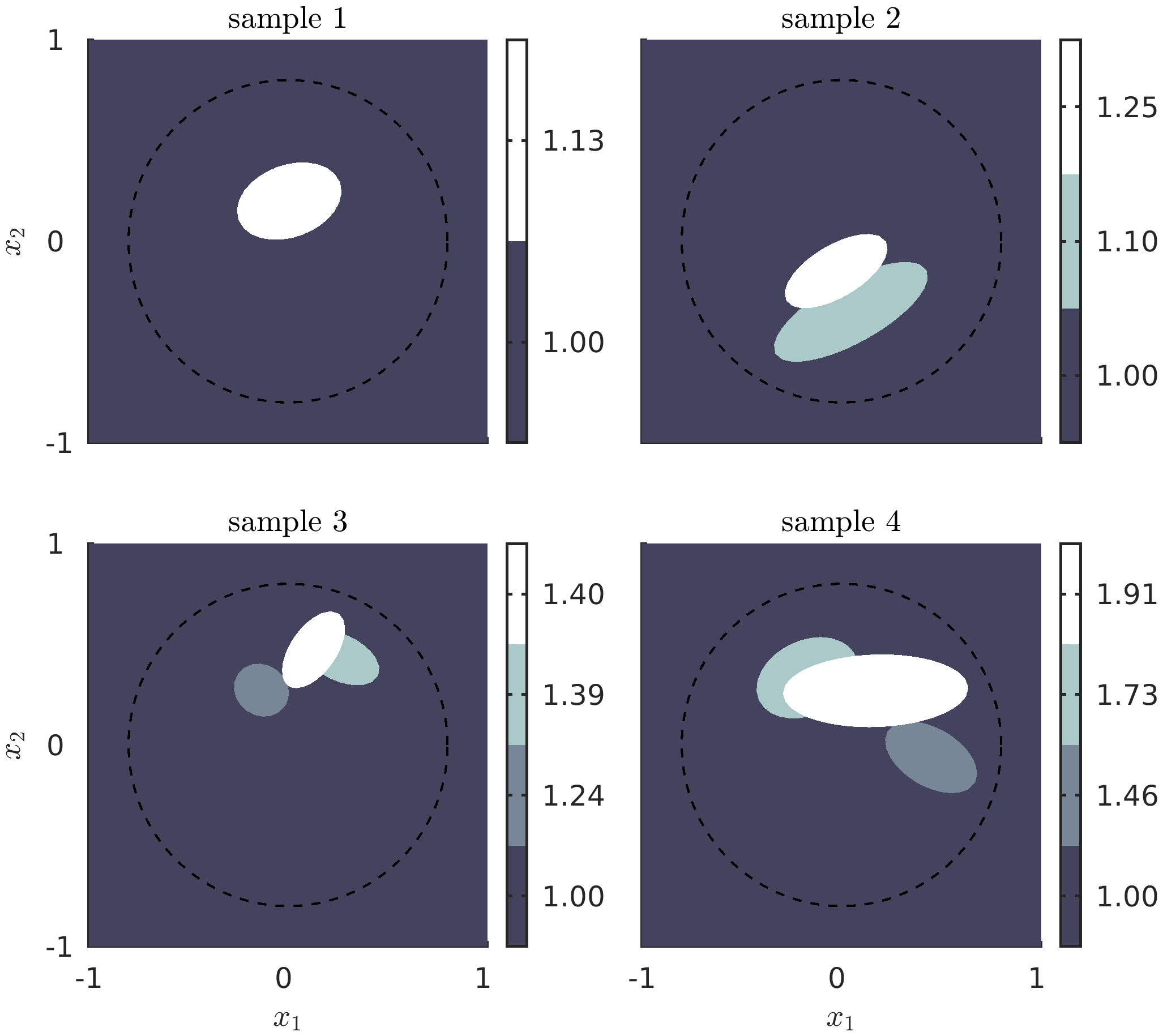
Figure 1: Four samples from $\bar{\pi}(\bar{n})$. The dashed line denotes the boundary $\partial D$.

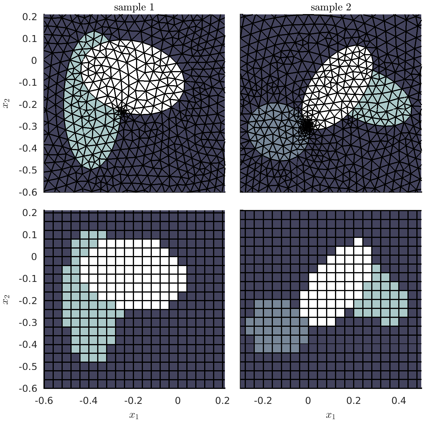
Figure 2: Two examples of draws from $\bar{\pi}(\bar{n}(\mbox{\boldmath$x$}))$ and the respective FEM meshes (top) and the corresponding Born grid and the projections $n=P\bar{n}$ (bottom). Left hand example: 10110 finite elements, 5176 vertices, $h_{\max}=0.06377$, $h_{\min}=0.00445$. Right hand example: 10362 finite elements, 5302 vertices, $h_{\max}=0.06377$, $h_{\min}=0.00271$. The Born grid is always a uniform $50\times 50$ grid.

4.3 Case 1: A single ellipsoidal scatterer

For each case, we compute the estimates of $n$ using the Born approximation with and without the Bayesian approximation error approach. In addition, with the BAE, we compute the estimates both with the full and the enhanced error models.

In this example, we have a single elliptic target with $\bar{n}=1.65$ inside the ellipse. The actual $\bar{n}$, and results for the Born, the full BAE and the enhanced error estimates are shown in Fig. 3. The contrast is relatively high and the Born approximation is inaccurate. This is seen in the estimate with an exaggerated size, with ringing and underestimated values of $\bar{n}$ inside the target (see top right panel of Fig. 3). The location of the target is approximately correct.

Both BAE estimates, on the other hand, estimate the size, the location and the values well. There is no significant ringing effect which would be due to the underestimation of the values within the target. Also the slightly elliptic shape of the target is roughly recognisable.

Two cross sections of the actual $\bar{n}$ and the three estimates are shown in Fig. 4. We also show the $\pm 1$ and $\pm 2$ posterior standard deviations along these cross sections. Qualitatively, the estimates exhibit the same characteristics as Fig. 3. In addition, most importantly, the BAE error estimates are useful in that the actual cross sections are within two posterior standard deviations of the reconstructions. This does not apply to the Born estimate. While one of the most significant assets of the Bayesian framework is that one can obtain posterior error estimates, this example shows that if any errors or uncertainties are not modelled (as is the case for the basic Born approximation shown in the top row of Fig. 4), the posterior error is typically underestimated.

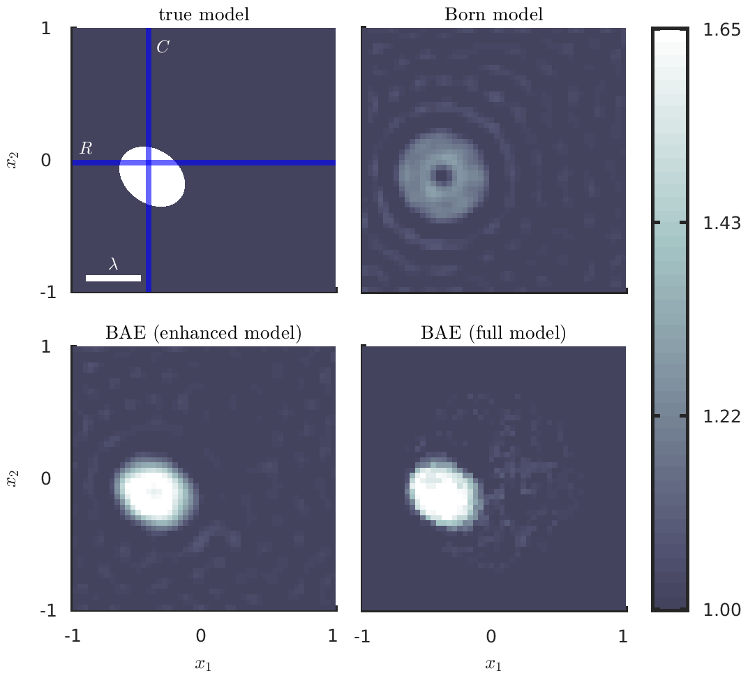
Figure 3: The reconstruction (estimates) of a single ellipsoidal scatterer with $\bar{n}=1.65$. Top left: the true $\bar{n}$. Top right: the standard Born approximation. Bottom left: the enhanced error model. Bottom right: the full BAE model. The wavelength $\lambda$ is indicated at the bottom left corner of the true model. The actual $\bar{n}$ and the reconstructions along the cross sections $R$ and $C$ are shown in Fig. 4.

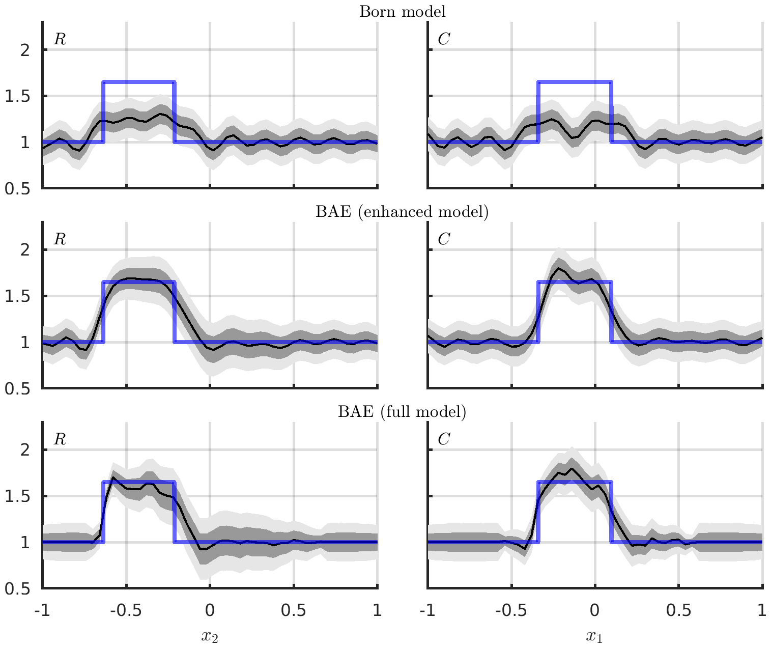
Figure 4: Estimates along the lines $R$ (left column) and $C$ (right column) for the single scatterer of Fig. 3. Transparent blue lines show the true model while black line shows the MAP-estimate. Dark grey denotes $\pm$1 standard deviation while light grey denotes $\pm$2 standard deviations.

4.4 Case 2: Three ellipsoidal scatterers

The second case contains three ellipsoidal scatterers for which the $\bar{n}$ values range from 1.3 to 1.6. The actual $\bar{n}$, the Born, the full BAE and the enhanced error estimates are shown in Fig. 5. Qualitatively, the results are similar to Case 1: The Born estimate has the general target location correctly but the target values are badly off and shapes (and the number of scatterers) are not recognisable. Again, both BAE estimates clearly exhibit the shapes, the values and the number correctly. Furthermore, in this case, the full error model is slightly better in estimating the gaps between the scatterers. Thus, employing the BAE error model seems to make it possible to handle, to a degree, also multiple scatterings between disjoint scatterers. The related cross sections are shown in Fig. 6. Again, the results are qualitatively similar to Case 1.

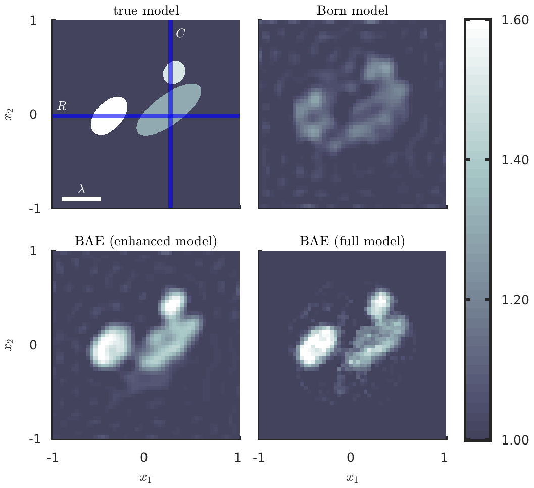
Figure 5: The reconstruction of a three ellipsoidal scatterers with the $\bar{n}$ values ranging from 1.3 to 1.6. The panels are as in Fig. 3. Top left: true scatterer. Top right: Born approximation. Bottom left: enhanced error model. Bottom right: full BAE. The actual $\bar{n}$ and the reconstructions along the cross sections $R$ and $C$ are shown in Fig. 6.

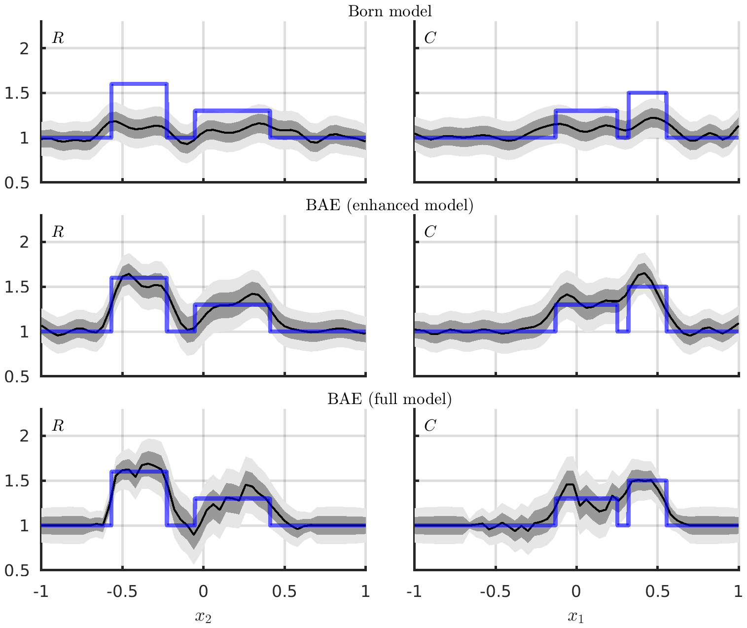
Figure 6: The estimates for three elliptic scatterers along cross sections $R$ and $C$ of Fig. 5. Left column: along $R$. Right column: along $C$.

4.5 Case 3: A resonant structure

The final target is a resonant structure shown in Fig. 7. The walls of the structure have the value $\bar{n}=1.7$, this value, the shape and the wavelength make the target a challenging case for the Born approximation, in particular, due to the evident multiple scatterings. While, in the previous cases, the actual targets were consistent with the prior model $\bar{\pi}(\bar{n})$ (1-3 random ellipsoidal scatterers), this example is not a feasible prior model. Thus this example serves as a test of the robustness of the approach. The estimates and the respective cross sections are shown in Figs. 7-8. In this case, the Born estimate is completely off exhibiting mere ringing, as was expected. On the other hand, both BAE estimates get both the shape and the values qualitatively correctly. Furthermore, the BAE results and their error estimates are useful, with the actual squared refractive index generally lying within $\pm$2 standard deviations of the reconstruction.

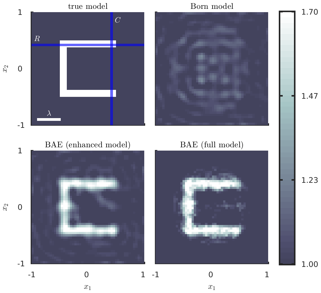
Figure 7: The reconstruction of a high contrast ($\bar{n}=1.7$) resonant structure. The layout of the figure is as in Fig. 3. The actual $\bar{n}$ and the reconstructions along the cross sections $R$ and $C$ are shown in Fig. 8.

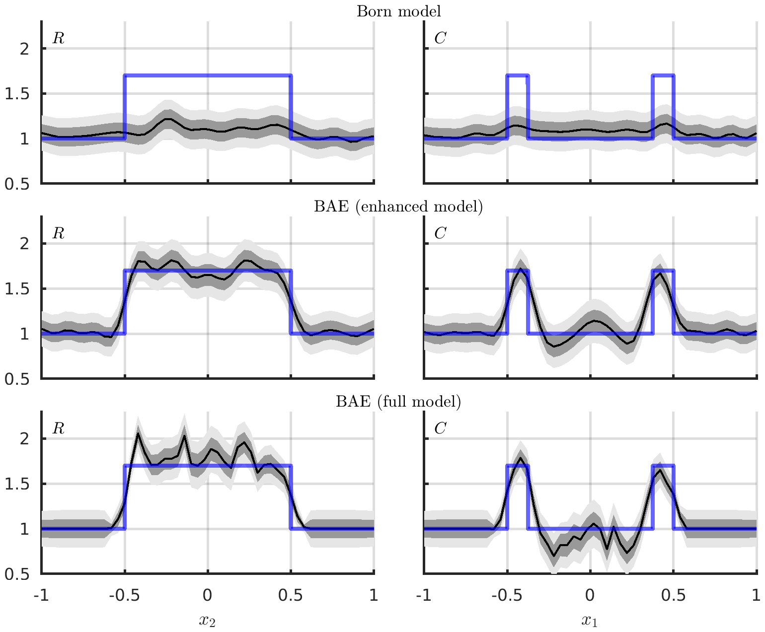
Figure 8: The estimates of $n$ for the cavity along lines $R$ and $C$ of Fig. 7. See Fig. 4 for an explanation of each panel.

5 Discussion

In this paper, we considered the time harmonic inverse scattering problem for a penetrable medium and the use of the Born approximation with high contrast and multiple scattering targets. It is well known that the computationally appealing Born approximation is not accurate for such scatterers.

We adopted the Bayesian approximation error approach to model the error that is induced by employing the Born approximation as the forward model. This approach models the statistics of the difference of the model predictions using an accurate and an approximate model. This approximation error appears in the observation model as a additive term that is correlated with the primary unknown. By carrying out a normal approximation to the joint distribution of the primary unknown and the approximation errors, this term can be marginalized analytically. This procedure yields a computationally efficient estimator that has the same or similar computational complexity as the Born estimator under normal models and, for example, a deterministic Tikhonov regularization.

The computational results suggest that the proposed approach can handle high contrast and multiple scattering targets. Most importantly, the posterior error estimates are found to be useful: the actual target typically lies within a few posterior standard deviation intervals.

References

- [1] G.S. Alberti, H. Ammari, F. Romero, and T. Wintz. Mathematical analysis of ultrafast ultrasound imaging. SIAM J. Appl. Math., 77:1–25, 2017.
- [2] S.R. Arridge, J. P. Kaipio, V. Kolehmainen, M. Schweiger, E. Somersalo, T. Tarvainen, and M. Vauhkonen. Approximation errors and model reduction with an application in optical diffusion tomography. Inverse Problems, 22:175–195, 2006.
- [3] G. Bao and P. Li. Inverse medium scattering problems for electromagnetic waves. SIAM J. Appl. Math., 65, 2015.
- [4] J.O. Berger. Statistical Decision Theory and Bayesian Analysis. Springer, 1980.
- [5] G.E.P. Box and G.C. Tiao. Bayesian Inference in Statistical Analysis. Wiley, 1992 (1973).
- [6] D. Calvetti, J. P. Kaipio, and E. Somersalo. Aristotelian prior boundary conditions. Int. J. Math., 1:63–81, 2006.
- [7] D. Calvetti and E. Somersalo. An Introduction to Bayesian Scientific Computing - Ten Lectures on Subjective Computing. Springer, 2007.
- [8] M. Cheney and B. Borden. Fundamentals of Radar Imaging. CBMS/SIAM, Philadelphia, 2009.
- [9] D. Colton and R. Kress. Inverse Acoustic and Electromagnetic Scattering Theory. Springer-Verlag, New York, 3rd edition, 2012.
- [10] A.J. Devaney. Mathematical Foundations of Imaging, Tomography and Wavefield Inversion. Cambridge University Press, Cambridge, UK, 2012.
- [11] J. Heino and E. Somersalo. A modeling error approach for the estimation of optical absorption in the presence of anisotropies. Phys. Med. Biol., 49:4785–4798, 2004.
- [12] J. Heino, E. Somersalo, and J. P. Kaipio. Compensation for geometric mismodelling by anisotropies in optical tomography. Opt. Express, 13(1):296–308, 2005.
- [13] T. Hohage. On the numerical solution of a three-dimensional inverse medium scattering problem. Inverse Problems, 17:1743–1763, 2001.
- [14] J.M.J. Huttunen and J.P. Kaipio. Approximation error analysis in nonlinear state estimation with an application to state-space identification. Inverse Problems, 23:2141–2157, 2007.
- [15] J. P. Kaipio and V. Kolehmainen. Approximate marginalization over modeling errors and uncertainties in inverse problems. In P. Damien, P. Dellaportas, N. G. Polson, and D. A. Stephens, editors, Bayesian Theory and Applications, chapter 32, pages 644–672. Oxford University Press, 2013.
- [16] J. P. Kaipio and E. Somersalo. Statistical and computational inverse problems. Applied Mathematical Sciences 160, Springer-Verlag, 2005.
- [17] J. P. Kaipio and E. Somersalo. Statistical inverse problems: Discretization, model reduction and inverse crimes. J. Comput. Appl. Math., 198:493–504, 2007.
- [18] V. Kolehmainen, T. Tarvainen, S. R. Arridge, and J. P. Kaipio. Marginalization of uninteresting distributed parameters in inverse problems: Application to diffuse optical tomography. Int. J. Uncertain. Quan., 2011.
- [19] J. Koponen, T. Huttunen, T. Tarvainen, and J. P. Kaipio. Bayesian approximation error approach in full-wave ultrasound tomography. IEEE T. Ultrason. Ferr., 61(10):1627–1637, 2014.
- [20] T. Lähivaara, N. F. Dudley Ward, T. Huttunen, J. P. Kaipio, and K. Niinimäki. Estimating pipeline location using ground-penetrating radar data in the presence of model uncertainties. Inverse Problems, 30(11):114006, 2014.
- [21] T. Lähivaara, N. F. Dudley Ward, T. Huttunen, J. Koponen, and J. P. Kaipio. Estimation of aquifer dimensions from passive seismic signals with approximate wave propagation models. Inverse Problems, 30(1):015003, 2014.
- [22] T. Lähivaara, N. F. Dudley Ward, T. Huttunen, Z. Rawlinson, and J. P. Kaipio. Estimation of aquifer dimensions from passive seismic signals in the presence of material and source uncertainties. Geophys. J. Int., 200:1662–1675, 2015.
- [23] A. Lehikoinen, S. Finsterle, A. Voutilainen, L. M. Heikkinen, M. Vauhkonen, and J. P. Kaipio. Approximation errors and truncation of computational domains with application to geophysical tomography. Inverse Probl. Imaging, 1:371–389, 2007.
- [24] P. Monk and E. Süli. The adaptive computation of far field patterns by a posteriori error estimation of linear functionals. SIAM J. on Numer. Anal., 36:251–74, 1998.
- [25] A. Nissinen, L. M. Heikkinen, and J. P. Kaipio. Approximation errors in electrical impedance tomography - an experimental study. Meas. Sci. Technol., 19, 2008.
- [26] A. Nissinen, L.M. Heikkinen, V. Kolehmainen, and J. P. Kaipio. Compensation of modelling errors due to unknown domain boundary in electrical impedance tomography. IEEE T. Med. Imaging, 30(2):231–242, 2011.
- [27] A. Nissinen, V. Kolehmainen, and J. P. Kaipio. Reconstruction of domain boundary and conductivity in electrical impedance tomography using the approximation error approach. Int. J. Uncertain. Quan., 1(3):203–222, 2011.
- [28] C.P. Robert and G. Cassella. Monte Carlo Statistical Methods. Springer, 2004.
- [29] F. Simonetti, L. Huang, N. Duric, and O. Rama. Imaging beyond the Born approximation: An experimental investigation with an ultrasonic ring array. Physical rev. E, 76, 2007. 036601.
- [30] A. Tarantola. Inverse Problem Theory and Methods for Model Parameter Estimation. SIAM, Philadelphia, 2004.
- [31] T. Tarvainen, V. Kolehmainen, J. P. Kaipio, and S. R. Arridge. Corrections to linear methods for diffuse optical tomography using approximation error modelling. Biomed. Opt. Express, 1(1):209–222, 2010.
- [32] T. Tarvainen, V. Kolehmainen, A. Pulkkinen, M. Vauhkonen, M. Schweiger, S. R. Arridge, and J. P. Kaipio. Approximation error approach for compensating modelling errors between the radiative transfer equation and the diffusion approximation in diffuse optical tomography. Inverse Problems, 26:015005, 2010.
- [33] P. Werner. Randwertprobleme der mathematischen Akustik. Arch. Rational Mech. Anal., 10:29–66, 1962.