The Expanded Giant Metrewave Radio Telescope

Abstract

With 30 antennas and a maximum baseline length of 25 km, the Giant Metrewave Radio Telescope (GMRT) is the premier low-frequency radio interferometer today. We have carried out a study of possible expansions of the GMRT, via adding new antennas and installing focal plane arrays (FPAs), to improve its point-source sensitivity, surface brightness sensitivity, angular resolution, field of view, and U-V coverage. We have carried out array configuration studies, aimed at minimizing the number of new GMRT antennas required to obtain a well-behaved synthesized beam over a wide range of angular resolutions for full-synthesis observations. This was done via two approaches, tomographic projection and random sampling, to identify the optimal locations for the new GMRT antennas. We report results for the optimal locations of the antennas of an expanded array (the “EGMRT”), consisting of the existing 30 GMRT antennas, 30 new antennas at short distances, $\lesssim 2.5$ km from the GMRT array centre, and 26 additional antennas at relatively long distances, $\approx 5-25$ km from the array centre. The collecting area and the field of view of the proposed EGMRT array would be larger by factors of, respectively, $\approx 3$ and $\approx 30$, than those of the GMRT. Indeed, the EGMRT continuum sensitivity and survey speed with $550-850$ MHz FPAs installed on the 45 antennas within a distance of $\approx 2.5$ km of the array centre would be far better than those of any existing interferometer, and comparable to the sensitivity and survey speed of Phase-1 of the Square Kilometre Array.

1 Introduction

At frequencies ranging from tens of MHz to hundreds of GHz, radio astronomy provides an outstanding and a unique window to study a wide range of astrophysical objects and phenomena. This includes pulsars, atomic, molecular and ionized gas in the Milky Way and other galaxies, the environments of supermassive black holes and accretion disk physics, jets and lobes from active galactic nuclei (AGNs), protoplanetary disks, complex organic molecules, solar and planetary emission, galaxy clusters, the cosmic microwave background, the epoch of reionization, etc. Over the last five decades, radio interferometers such as the Westerbork Synthesis Radio Telescope (WSRT), the Very Large Array (VLA), the Australia Telescope Compact Array (ATCA), the Very Long Baseline Array (VLBA), etc., consisting of multiple dishes spread over distances much larger than the dish size, have used the technique of earth-rotation aperture synthesis (McCready, Pawsey & Payne-Scott, 1947; Ryle, 1952; O’Brien, 1953) to obtain angular resolutions many orders of magnitude finer than would have been possible with even the largest single dish radio telescopes. Such telescopes have yielded detailed information on the structure and kinematics of Galactic and extra-galactic radio sources and have dramatically improved our understanding of the Universe. More recently, over the last few years, there has been a dramatic upsurge in radio astronomy, with new interferometers such as the Atacama Large Millimeter/sub-millimeter Array (ALMA; Wootten & Thompson, 2009) at high frequencies ($\gtrsim 100$ GHz), and the Low Frequency Array (LOFAR; van Haarlem et al., 2013) and the Murchison Widefield Array (MWA; Tingay et al., 2013) at very low frequencies ($\lesssim 300$ MHz). In parallel, there have been significant upgrades to the VLA, resulting in the Karl G. Jansky VLA (JVLA) which has outstanding sensitivity and frequency coverage at intermediate frequencies $\approx 1-50$ GHz (e.g. Perley et al., 2011). New or upgraded interferometers with wide fields of view and survey speed, such as the Australian SKA Pathfinder (ASKAP; e.g. Johnston et al., 2008), the MeerKAT array (e.g. Booth et al., 2009), and the APERTIF system on the WSRT (e.g. Verheijen et al., 2008) are being commissioned today. Finally, the next generation radio interferometer, the Square Kilometre Array (SKA), of unparalleled sensitivity, is currently being designed, aiming for completion in the next decade (e.g. Dewdney et al., 2015).

The Giant Metrewave Radio Telescope (GMRT; Swarup et al., 1991) is one of the leading radio interferometers in the world today. Completed around 20 years ago, the GMRT consists of 30 parabolic dishes, each of 45-m diameter, and with a longest baseline of $\approx 25$ km. Fourteen of the GMRT antennas are located within a “central square”, of size $\approx 1\;{\rm km}\;\times 1$ km, while the remaining 16 antennas are distributed along three arms of a Y, each of $\approx 12$ km length. This hybrid configuration, shown in Fig. 1, with both closely-separated and distant antennas, yields good U-V coverage out to the longest antenna separations (i.e. $\approx 25$ km) over a full-synthesis track, and thus simultaneously provides information on radio emission at both small and large angular scales. The GMRT’s observing frequencies lie in the range $\approx 150-1450$ MHz, with the upper range overlapping with the lower range of the VLA ($\approx 1-50$ GHz). The two arrays thus provide complementary views of the Universe, over a wide and contiguous range of frequencies.

The GMRT has produced outstanding science in a wide range of areas, including pulsar studies (e.g. Gangadhara & Gupta, 2001; Freire et al., 2004; Hermsen et al., 2013; Bhattacharyya et al., 2013, 2016; Roy et al., 2015), Hi 21 cm spectroscopy of dwarf galaxies (e.g. Begum et al., 2006, 2008; Roychowdhury et al., 2010), Hi 21 cm and hydroxyl (OH) absorption studies of high-redshift galaxies (e.g. Kanekar & Chengalur, 2002, 2003; Kanekar et al., 2009, 2014), studies of AGNs and their environments (e.g. Ishwara-Chandra, Dwarakanath & Anantharamaiah, 2003; Gupta et al., 2006; Lal & Rao, 2007; Aditya, Kanekar & Kurapati, 2016), studies of galaxy clusters (e.g. Venturi et al., 2007, 2008; Brunetti et al., 2007, 2008; Giacintucci et al., 2011; van Weeren et al., 2010; Kale et al., 2015; van Weeren et al., 2017), physical conditions in atomic gas in the Milky Way (e.g. Kanekar, Braun & Roy, 2011; Roy, Kanekar & Chengalur, 2013), extra-galactic continuum studies (e.g. Garn et al., 2007; Ibar et al., 2009; Ishwara-Chandra et al., 2010; Mauch et al., 2013; Taylor & Jagannathan, 2016), Galactic Plane studies (e.g. Bhatnagar, 2000; Chengalur & Kanekar, 2003; Roy & Pramesh Rao, 2004; Roy, 2013), studies of transient sources (e.g. Vadawale et al., 2003; Chandra, Ray & Bhatnagar, 2004; Hyman et al., 2009; Roy et al., 2010; Chandra & Kanekar, 2017), giant radio sources (e.g. Bagchi et al., 2007, 2014; Tamhane et al., 2015; Sebastian et al., 2018), Hi 21 cm emission stacking studies of cosmologically-distant galaxies (e.g. Lah et al., 2007, 2009; Kanekar, Sethi & Dwarakanath, 2016; Rhee et al., 2016), constraints on fundamental constant evolution (e.g. Chengalur & Kanekar, 2003; Kanekar et al., 2010), all-sky surveys (Intema et al., 2017), studies of the epoch of reionization (e.g. Paciga et al., 2011, 2013), etc. At present, the GMRT is the premier telescope in the world in terms of sensitivity and angular resolution at low frequencies, $\lesssim 1$ GHz, and, indeed, has the largest collecting area of any fully steerable telescope at all frequencies.

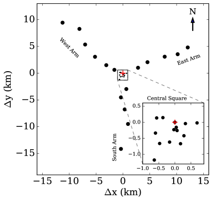
Figure 1: The GMRT array, with antenna locations shown by the filled circles. The 30 GMRT antennas are arranged in a “Y” array, consisting of 14 antennas in a central core (the “central square”), and the remaining 16 antennas in the three arms (“West”, “East”, and “South”) of the Y. The red “+” sign indicates the nominal origin of the array, at antenna C02.

2 The Upgraded GMRT

All of the above studies were based on observations with the original GMRT, with a maximum bandwidth of $\approx 32$ MHz, and with narrow frequency bands, covering $\approx 150-156$ MHz, $\approx 230-245$ MHz, $\approx 300-360$ MHz, $\approx 570-660$ MHz, and $\approx 900-1450$ MHz. The GMRT is currently being upgraded, with the installation of new receivers covering $\approx 125-250$ MHz, $\approx 250-500$ MHz, $\approx 550-850$ MHz, and $\approx 950-1450$ MHz (i.e. near-seamless coverage over $\approx 125-1450$ MHz), and a new wideband correlator with a bandwidth of 400 MHz (Gupta et al., 2017). This will result in a significant increase in the telescope sensitivity (by a factor of $\approx 3$) for continuum and pulsar studies, in the U-V coverage of the array for continuum studies of complex sources, and in the frequency coverage for studies of redshifted Hi 21 cm and OH emission and absorption, and radio recombination lines. Indeed, the installation of the first few GMRT $250-500$ MHz receivers resulted in two new detections of redshifted Hi 21 cm absorption at $z\approx 2$ (Kanekar, 2014).

Fig. 2 compares the continuum sensitivity [i.e. the root-mean-square (RMS) noise] of the upgraded GMRT (the “uGMRT”) for a 9-hour full-synthesis integration with the sensitivities of the best radio interferometers in the world, at frequencies $\lesssim 10$ GHz. The figure includes existing interferometers (the uGMRT, the JVLA, and LOFAR), interferometers that are now coming online (MeerKAT and ASKAP) and Phase 1 of the SKA (labelled “SKA-1”). It also includes the $1\sigma$ source confusion limit (see Section 3.4) of the uGMRT at its different observing frequencies, shown as the magenta dashed line (using equation 27 of Condon et al., 2012). The black dashed line shows the spectrum of a typical extra-galactic source emitting optically-thin synchrotron radiation, with a spectral index of $\alpha=-0.7$ (assuming that the source flux density $S_{\nu}\propto\nu^{\alpha}$). It is clear that the continuum sensitivity of the uGMRT over the frequency range $\approx 300-1400$ MHz will be sufficient to detect all typical synchrotron-emitting sources detected by the JVLA at frequencies $\gtrsim 1$ GHz; the two telescopes will thus continue to complement each other. However, it is also clear that the sensitivity of the uGMRT at frequencies below 500 MHz will be limited by source confusion in even relatively short integrations. Further, the MeerKAT array will have a sensitivity (limited by source confusion) comparable to that of the uGMRT (and the JVLA) at frequencies $\gtrsim 1$ GHz, while the SKA-1 would have a far better sensitivity than the uGMRT throughout its frequency range.

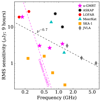
Figure 2: The $1\sigma$ continuum noise of the uGMRT (in magenta stars) as a function of observing frequency, compared with the sensitivity of the best current and planned radio interferometers in the world [JVLA in grey stars, LOFAR in red circles, MeerKAT (in cyan triangles) , ASKAP (in black asterisks) and the SKA-1 (orange squares)], for a 9-hour full-synthesis integration. The dashed magenta line shows the $1\sigma$ GMRT confusion noise at the different observing frequencies. The dashed black line shows the spectral energy distribution of a typical synchrotron-spectrum extragalactic continuum source, with flux density $\propto\nu^{-0.7}$. The continuum sensitivities are from the webpages of the various telescopes or, for existing arrays like the JVLA, from their Exposure Time Calculators; note that the sensitivity of the MeerKAT array will be limited by source confusion, especially at frequencies $\lesssim 1$ GHz. See main text for discussion.

Another important metric characterizing a modern radio telescope is survey speed; the large diameter of the GMRT dishes imply that the uGMRT’s survey speed figure of merit is lower than that of an interferometer like MeerKAT which has smaller dishes, and far lower than that of ASKAP, which has both smaller dishes and phased-array feeds (see, e.g., Table 1 of Dewdney et al., 2015). Wide-field surveys would thus require a far larger number of uGMRT telescope pointings and thus a concomitant increase in observing time.

Finally, the increased GMRT bandwidth has meant a significant improvement in sensitivity for both continuum and pulsar studies. However, while the improved frequency coverage implies a significant increase in the redshift range accessible for GMRT studies in the redshifted Hi 21 cm and OH lines, there has been no increase in the sensitivity for such spectral line studies. This would only be possible by increasing the number of antennas and/or by decreasing the system temperature.

In summary, while the uGMRT will definitely yield outstanding science over the next decade, it is important to begin considering the next expansion of the telescope, to retain its importance in the SKA era. In this paper, we discuss different strategies for an expanded GMRT (the “EGMRT”) and their science benefits, and finally describe the results of array configuration studies for the locations of the new antennas of the expanded array.

3 The Expanded GMRT

We assume that the frequency coverage of the GMRT will remain approximately unchanged in the expansion (except possibly for a minor extension to lower frequencies, $<100$ MHz). This is because the mesh spacing of the current GMRT antennas would imply a rapid drop in sensitivity at frequencies $\gtrsim 2$ GHz. Note that a reduction in the mesh spacing of the existing GMRT antennas would increase the wind loading, and hence could affect the structural stability of the dishes. We first consider the basic issue of the point-source sensitivity of the present GMRT and compare this with the sensitivities of current and planned arrays. We then considered three possible avenues for the expansion of the GMRT, to achieve (1) a wider field of view, (2) improved surface brightness sensitivity, and (3) improved angular resolution, and hence a better confusion limit. The broad science drivers and possible challenges for each of these approaches are discussed in brief in the present section.

3.1 Point Source Sensitivity

The original GMRT was built with the aim of being sufficiently sensitive to detect Hi 21 cm line emission from neutral hydrogen from massive proto-clusters at $z\approx 3$, a prediction of the hot dark matter cosmological model (Swarup et al., 1991). The continuum sensitivity was sufficient to provide a low-frequency counterpart to the original higher-frequency VLA, allowing the detection at frequencies $\lesssim 1.4$ GHz of synchrotron emission from extragalactic sources detectable with the VLA at frequencies $\gtrsim 1.4$ GHz. It can be seen from Fig. 2 that the uGMRT will provide a similar low-frequency counterpart to the JVLA, with comparable continuum sensitivity at $\approx 1.4$ GHz. However, it is also clear from the figure that the uGMRT will have a far lower sensitivity than SKA-1 at all frequencies. While SKA-1 is likely to be built in the southern hemisphere, leaving the northern hemisphere niche for the uGMRT, increasing the point-source sensitivity of the GMRT is critical for it to remain competitive over the next decade, in the SKA era. Fig. 2 shows that this would require roughly a tripling of the uGMRT sensitivity.

3.2 Focal plane arrays: An increased field of view

The GMRT currently has single-pixel feeds, and hence, a relatively small field of view, implying a low survey speed, even with the wider bandwidths of the uGMRT. In recent years, much emphasis has been placed on the development of focal plane arrays (FPAs) with relatively low system temperatures (e.g. van Ardenne et al., 2009; DeBoer et al., 2009; Chippendale et al., 2016), to obtain both a wide field of view and a high point-source sensitivity. L-band FPAs covering $\approx 1000-1700$ MHz have been installed on the WSRT (the APERTIF system; e.g. Verheijen et al., 2008) and the new ASKAP array (e.g. Johnston et al., 2008), each with 30 independent beams on the sky, resulting in far higher survey speeds than at the GMRT (see Table 1 of Dewdney et al., 2015). Such an FPA system, with $\approx 30$-beams, would imply a huge jump in the GMRT’s field of view. We note that the GMRT’s prime-focus feeds are uncooled, with relatively high system temperatures, $T_{\rm sys}\approx 70-100$ K at $300-1450$ MHz. The high point-source sensitivity of the GMRT arises due to its large collecting area; the installation of FPAs on the GMRT would hence not give much of a penalty in system temperature.

The main science drivers for an FPA system on the GMRT are Hi 21 cm, pulsar, and continuum surveys, and the exciting new field of radio transients, especially fast radio bursts (FRBs; e.g. Lorimer et al., 2007; Thornton et al., 2013; Spitler et al., 2016). While a low-frequency FPA (at $\lesssim 500$ MHz) would significantly increase the GMRT survey speed, benefitting radio continuum and pulsar surveys, it is very unlikely to be possible to detect redshifted Hi 21 cm emission from individual galaxies at $z\gtrsim 1.8$, for which the Hi 21 cm line would redshift to frequencies $\lesssim 500$ MHz. Further, while initial studies were unable to detect FRBs at frequencies $\lesssim 800$ MHz (e.g. Petroff et al., 2016), FRBs have recently been detected at frequencies $\gtrsim 400$ MHz with the Canadian Hydrogen Intensity Mapping Experiment (Boyle & Chime/Frb Collaboration, 2018). The two broad frequency ranges of interest for an FPA system on the GMRT are hence likely to be $\approx 1000-1400$ MHz and $\approx 550-850$ MHz. FPAs covering the former frequency range have already been installed on the WSRT and ASKAP arrays; the best science outcomes for the GMRT are hence likely to be obtained from an FPA covering the relatively unexplored frequency range of $\approx 550-850$ MHz. The large field of view and frequency coverage of such a system, coupled with GMRT’s high sensitivity, would yield a large instantaneous survey volume, allowing one to detect Hi 21 cm emission from individual massive galaxies at $z\approx 0.6-1.5$. Optical studies of star-forming galaxies have shown that the cosmic star formation rate (SFR) density of the Universe peaks in the redshift range $\approx 1-3$, often referred to as the “epoch of galaxy assembly”, before declining by an order of magnitude to the present epoch (e.g. Hopkins & Beacom, 2006; Bouwens et al., 2014). However, little is known about atomic gas in these galaxies, the fuel for such star formation. The GMRT single-pixel feeds have been used to obtain an upper limit on the average gas mass of star-forming galaxies at $z\approx 1.3$, by co-adding their Hi 21 cm emission signals (Kanekar, Sethi & Dwarakanath, 2016), but the GMRT field of view is too small to carry out a survey for Hi 21 cm emission from massive galaxies at these redshifts in reasonable observing time. The prospect of using FPAs covering $550-850$ MHz on the GMRT to trace the evolution of atomic gas in star-forming galaxies from the peak epoch of star formation down to intermediate redshifts is hence a very exciting one (Patra et al., in prep.). Of course, a 30-beam FPA system at these frequencies would yield a field of view of $\approx 15$ square degrees at $\approx 600$ MHz, allowing wide-field high-sensitivity surveys for pulsars, FRBs, and extra-galactic continuum sources.

The main challenges in installing FPAs on the GMRT are the large data volumes, signal transport (especially bringing a large number of signal-carrying cables from the individual FPA elements to the base of each antenna), digital signal processing, the possibility of RFI on short baselines, and supporting an FPA at the prime focus of the GMRT antennas. None of these appear intractable at this time. We note, in passing, that, since the FPAs are likely to be installed mostly on the shorter-baseline antennas (see below), land acquisition is unlikely to be a critical issue for this expansion route.

3.3 Short baselines: Surface brightness sensitivity

The GMRT currently has few antennas at distances $\lesssim 0.2$ km from each other, and hence has relatively poor U-V coverage at short U-V spacings, which adversely affects its ability to image extended, large-scale radio emission. Indeed, we note that the GMRT has only three baselines with a physical separation $<100$ m. This is a serious limitation for studies of complex fields in the Galactic plane, and especially of the exciting region around the Galactic Centre (e.g. Anantharamaiah et al., 1991; LaRosa et al., 2000; Nord et al., 2004; Yusef-Zadeh, Hewitt & Cotton, 2004). Radio relics and halos in galaxy clusters are also typically very extended, requiring good U-V coverage at short spacings to both detect the emission and study its physical properties (e.g. Venturi et al., 2007; Brunetti et al., 2008; Deo & Kale, 2017). Detecting “cosmological halos” of ionized gas around massive high-$z$ quasars would also require a large collecting area at short baselines (e.g. Sholomitskii & Yaskovich, 1990; Geller et al., 2000). Adding new antennas with short physical separations ($\ll 1$ km) to the GMRT would significantly improve its surface brightness sensitivity. Of course, both Hi 21 cm emission and pulsar surveys would benefit from adding antennas at such short spacings. In the case of Hi 21 cm emission studies of external galaxies, new antennas at short spacings would not resolve out the emission. Conversely, for pulsar surveys, the number of phased-array beams needed to cover the full primary beam would be very large if one were to include long-baseline antennas (e.g. Roy, 2018); further, antennas on short baselines would be easier to phase up for pulsar searches.

The primary challenge for the short-baseline expansion is likely to be RFI, which would not decorrelate on short baselines. We note that RFI has been a steadily worsening problem at the GMRT over the last decade and that online RFI mitigation techniques (e.g. Buch et al., 2016) will be critical to deal with this issue. Since the observatory already owns most of the required land for the short-baseline expansion (for baselines $\lesssim 1.7$ km; see Section 4.2), land acquisition is unlikely to be a serious problem here.

3.4 Long baselines: The confusion limit

The maximum attainable angular resolution of an aperture synthesis radio telescope is decided by its longest baseline. The GMRT currently has a longest baseline of $\approx$ 25 km, which implies an angular resolution of $\approx 3^{\prime\prime}/[\nu/{\rm GHz}]$ . This angular resolution sets the “confusion limit” of the array, the RMS noise arising due to the blending of multiple faint individually-undetected sources within the array synthesized beam (e.g. Mills & Slee, 1957; Mitchell & Condon, 1985; Condon et al., 2012). It has long been appreciated that source confusion plays an important role in determining the continuum sensitivity of a synthesis telescope (e.g. Mills & Slee, 1957; Scheuer, 1957); for deep continuum images, the detection threshold is set by a combination of the theoretical RMS noise and the confusion noise.

For fifty years, arrays have mostly been designed so as to not be limited by source confusion. However, the huge increase in the bandwidth of existing radio telescopes, due to advances in signal transport methods and correlator capacity, without a corresponding increase in the baseline length has meant that the continuum sensitivity of today’s interferometers is often limited by source confusion at low frequencies ($\lesssim 1$ GHz), rather than by the theoretical RMS noise. The best estimate of the low-frequency confusion limit can be obtained by extrapolating equation (27) of Condon et al. (2012)

$$\rm\sigma_{c}^{*}\approx 1.2\mu JyBeam^{-1}\left[\frac{\nu}{3.02\;GHz}\right]^{-0.7}\left[\frac{\theta}{8^{\prime\prime}}\right]^{10/3}$$ (1)

to the observing frequency, $\nu$, where $\theta$ is the full-width-at-half-maximum (FWHM) of the array synthesized beam, and $5\sigma_{c}^{*}$ gives an estimate of the source detection threshold due to confusion. Note that $\sigma_{c}^{*}$ is not the rms confusion noise (see the discussion in Condon et al., 2012, for the definition of $\sigma_{c}^{*}$); indeed the distribution is highly skewed so the RMS confusion noise does not give a good estimate of the detection threshold (Condon et al., 2012). For the GMRT, this implies $\rm\sigma_{c}^{*}\approx 0.052\times(\nu/1\;{\rm GHz})^{-4.0}$, i.e. a $5\sigma$ detection threshold of $\approx 24~{}\mu$Jy at 327 MHz. This was not a serious issue for the original GMRT , with a bandwidth of 32 MHz, as the $5\sigma$ detection threshold in a full-synthesis 327 MHz run was $\approx 50\;\mu$Jy, implying that full-synthesis 327 MHz images were not significantly limited by source confusion. However, it is clear from Fig. 2 that $\rm\sigma_{c}^{*}$ is comparable to the theoretical RMS noise at $\approx 400$ MHz for a full-synthesis run, implying that the uGMRT would be limited by source confusion in the $250-500$ MHz band for observing times $\approx 10$ hours. The only way to address this issue is to increase the angular resolution of the array, by installing antennas at long baselines, $>25$ km. The strong dependence of $\rm\sigma_{c}^{*}$ on the FWHM of the synthesized beam ($\sigma_{c}^{*}\propto\theta^{10/3}$; Condon et al., 2012) implies that merely doubling the angular resolution reduces the confusion limit by an order of magnitude. Specifically, increasing the length of the longest GMRT baseline to $\approx 50$ km would reduce $5\sigma_{c}^{*}$ at 400 MHz to $\approx 2.3~{}\mu$Jy, below the theoretical RMS noise ($\approx 3~{}\mu$Jy) in a full-synthesis uGMRT observation at a central frequency of 400 MHz. Doubling the length of the longest GMRT baseline would thus render source confusion an issue only for extremely deep 400-MHz integrations ($\gg 100$ hours). We will hence use 50 km as the target length of the longest baseline of the expanded array.

Acquiring the land needed for the installation of the new antennas is likely to be the biggest challenge for the long-baseline expansion. We are currently carrying out a land survey for this purpose, to identify tracts of land that might be used as antenna sites. Signal transport from the distant antennas is unlikely to be a serious problem, while RFI, although always an issue, should have its weakest effects on the long baselines.

3.5 The Proposed Expanded GMRT

The original GMRT was also designed to be suitable for multiple science goals, and hence has roughly half its collecting area in the central regions and half on the long baselines, out to 25 km. The former is useful for Hi 21 cm emission studies of nearby galaxies and pulsar studies, besides providing acceptable surface brightness sensitivity for Galactic plane studies, while the latter yields the angular resolution needed to overcome source confusion and produce deep images of extra-galactic fields, as well as spatially-resolved information on individual sources like radio galaxies or galaxy clusters. In the case of the expanded GMRT, we aim to increase the point-source sensitivity by a factor of $\approx 3$, by adding new antennas to the array. Further, as discussed in Sections 3.3 and 3.4, there are excellent science arguments for adding the new antennas on both short and long baselines. Since none of these science drivers appears to dominate over the others, we plan to retain GMRT’s multi-science capabilities, and distribute the new antennas on both short and long baselines, so as to significantly improve the surface brightness sensitivity, the sensitivity to high-$z$ Hi 21 cm emission, the pulsar sensitivity, and the confusion limit. This may be accomplished by adding roughly half the new collecting area (i.e. $\approx 30$ antennas) in a central region of size $\approx 5$ km, aiming to use this to provide excellent sensitivity for high-$z$ Hi 21 cm emission studies, pulsar studies, and Galactic plane studies, and the remaining $\approx 30$ new antennas on intermediate and long baselines, to improve the angular resolution by a factor of $\approx 2$, and thus improve the confusion limit by a factor of $\approx 10$. This approach would triple the EGMRT’s point-source sensitivity relative to that of the uGMRT, while also significantly improving both its surface brightness sensitivity and confusion limit.

Next, it appears clear that installing FPAs with $\approx 30$ beams will be critical to obtaining a high survey speed, especially given the fact that the large diameter of the GMRT antennas implies a relatively small field of view for single-pixel feeds. Installing a 30-beam FPA on the full array would imply serious problems in signal transport from the more distant antennas to the central correlator. However, none of the main science drivers for a $550-850$ MHz FPA system (pulsar surveys, Hi 21 cm emission from galaxies at $z\approx 0.6-1.5$, wide-field continuum surveys, and searches for fast radio transients) require the FPAs to be installed on long-baseline antennas. Installing a 30-beam FPA system on the core antennas of the new array, out to maximum baselines of $\approx 5-10$ km, would alleviate the signal transport issue. The confusion limit for wide-field continuum surveys with this sub-array, assuming a maximum baseline of $\approx 10$ km and equation (27) of Condon et al. (2012), would give a $5\sigma$ detection threshold of $\rm 5\sigma_{c}^{*}\approx 23~{}\mu$Jy at 700 MHz.

4 The EGMRT Antenna Configuration

As discussed in the previous section, we would like to explore the possibility of increasing the sensitivity of the uGMRT by a factor of $\approx 3$, by adding $\approx 30$ antennas in a central region, of size $\lesssim 10$ km, and a further $\approx 30$ antennas out to baselines of $\approx 50$ km. In order to significantly improve the surface brightness sensitivity, one has to also increase the number of antennas on very short spacings $\ll 1$ km. Our next step is to identify the locations of the proposed new antennas. The critical requirement here is that the antenna configuration provides a good U-V coverage, with no holes in U-V space that might give rise to high sidelobes in the array point spread function and hence, artefacts when imaging complex fields. Our aim is hence to identify an antenna configuration that yields a synthesized beam as close to an “ideal” beam as possible. We will use a 2-dimensional (2-D) circular Gaussian synthesized beam as the ideal beam for all configurations. Since the U-V coverage is the 2-D Fourier transform of the synthesized beam, we aim to obtain a U-V distribution as close to a 2-D Gaussian as possible, with an appropriate choice of the FWHM of this 2-D Gaussian. We then rank antenna configurations based on the fractional RMS difference between the actual 2-D U-V distribution and the ideal 2-D Gaussian distribution, aiming to minimize this fractional RMS difference. This quantity, expressed as a percentage, will be referred to as the “Residual RMS”; note that a lower Residual RMS implies a better agreement between the actual and the ideal U-V configuration, and hence a preferred antenna configuration.

It is important to also emphasize that, unlike in the case of a new array such as MeerKAT, ASKAP, or the SKA, we will be adding antennas to an existing array. This complicates the minimization procedure as the locations of the existing GMRT antennas must be frozen in the minimization.

We have alluded above to the critical issue of land availability in the area around the GMRT, an important constraint for the optimization. The GMRT already owns some land around the existing central square, out to baselines of $\approx 1.7$ km, that might immediately be used for an expansion. It should be possible to select the preferred antenna sites here, based on the simulations below for the optimal U-V coverage. We are currently carrying out a survey to identify land that may be acquired for the purpose of expanding the GMRT; this survey is now complete out to a region of $\approx 5$ km diameter around the central square. Land in the above two categories, i.e. either already owned by the GMRT or owned by the government and that might be acquired for the array expansion, was included in the allowed antenna locations in the simulations out to baselines of $\approx 5$ km. However, we emphasize that changes may be needed in the antenna configuration identified below, in case it is not possible to acquire individual locations. Finally, for baselines longer than $5$ km, we have chosen to identify the optimal antenna location via the present simulations. We note that, for the long-baseline antennas, the exact location of each individual antenna (within $\approx 1$ km) is unlikely to have a significant impact on the U-V coverage, and hence on the synthesized beam. We hence plan to carry out a land survey within $\approx 1$ km of each new optimal antenna location determined below to identify government land that might be acquired for the final antenna locations. We emphasize that the antenna locations identified by the approach below may not be the final ones, especially for the long-baseline antennas; however, the inferred antenna configurations will serve as a benchmark to test possible array configurations based on the final land surveys, and additional constraints arising from optical fibre connectivity, accessibility, etc.

4.1 The two approaches: Random sampling and Tomographic projection

Many approaches exist in the literature to the problem of optimizing antenna locations for radio synthesis arrays (e.g. Keto, 1997; Boone, 2001; de Villiers, 2007). We have chosen to use two separate, and independent, schemes to identify the array configuration that minimizes the Residual RMS. The first, applicable to relatively small areas (e.g. to the short- and intermediate-baseline configurations), is based on a simple Monte Carlo approach, in which we set up a grid of allowed antenna locations and then determine the Residual RMS for a large number (typically, $10^{4}$) of array configurations using random sampling of the possible locations, including any constraints based on land availability. The array configuration that yields the minimum Residual RMS is selected as the best configuration; we will refer to this as “random sampling”. This method is computationally expensive, but is guaranteed to yield the best configuration, given a sufficiently large number of random samples, and hence works well for small areas where it is possible to sample a large fraction of the possible array configurations.

The second approach, referred to as “tomographic projection”, is based on reducing the problem of two-dimensional U-V coverage to a one-dimensional problem, by taking random projections of the two-dimensional antenna distribution along different angles and then moving the antennas so as to minimize the difference between the U-V distribution in one dimension (for each projection) and an ideal distribution (de Villiers, 2007). The antenna locations are shifted for each projection direction, until one obtains an acceptable two-dimensional U-V coverage, and hence, an acceptable synthesized beam. Note that the minimization procedure is complicated by the fact that one would like the U-V points (i.e. the baseline distribution) to have an ideal distribution, but moving an antenna to shift a single U-V point also shifts all the other U-V points arising from that antenna (i.e. the U-V points are not independent; de Villiers, 2007).

The tomographic projection algorithm has been implemented in the iAntConfig software package; we used this to optimize our antenna layouts. However, we found that the results of the iAntConfig optimization are sensitive to the initial conditions, and that more stable results are obtained by combining the iAntConfig minimization procedure with a Monte Carlo approach, running iAntConfig $\approx 100$ times for different initial antenna configurations. We evaluated the Residual RMS for each of the iAntConfig output layouts, each with the difference between the actual and ideal U-V distributions minimized using tomographic projection, and chose the antenna configuration with the lowest value of the Residual RMS. We tested the results of this approach against those from the random sampling procedure for small regions (where the random sampling procedure is reliable), and found that the two approaches yielded very similar array configurations.

We note, in passing, that the tomographic projection approach is significantly less computationally intensive than the random sampling method, and thus appears far better suited for optimizing array configurations. However, it is not straightforward to include constraints on land availability in the tomographic projection optimization. The current implementation in iAntConfig carries out the optimization without including land constraints, and applies the land constraint at the end, by shifting the antenna locations to the nearest available ones. For sparse land availability (as is the case around the GMRT), this does not guarantee a minimum Residual RMS. The random sampling approach is not adversely affected by land constraints and, in fact, works better for sparse land availability because the number of allowed antenna locations is significantly reduced, making it possible to sample a larger fraction of possible array configurations. We hence chose to use the random sampling approach for the short- and intermediate-baseline antenna locations, but to use tomographic projection for the long-baseline locations.

4.2 Inputs for the optimization

The critical inputs for the optimization are the observing frequency, the bandwidth, the number of channels, the time resolution, the total integration time, and the target declination. We chose to carry out the optimization at $\approx 1.2$ GHz in GMRT’s highest observing frequency band, since the fractional bandwidth here is the worst for a given observing bandwidth. This implies the worst U-V coverage of all GMRT bands, and hence emphasizes any holes in the U-V coverage.

We carried out the optimization for different time resolutions, to examine the effects of the selected sampling time on the derived array configurations. Of course, high temporal resolution would require significantly more computational time. No significant difference in the final array configuration was obtained on using resolutions finer than $\approx 120$ seconds. We hence finally used time resolutions of $\approx 120-180$ seconds for all optimizations, with the coarsest time resolution used for the shortest baseline configurations, and $120$ seconds used for all other optimizations.

Next, a large fractional bandwidth significantly improves the U-V coverage of a radio interferometer. The fractional bandwidth of the uGMRT ranges from $\approx 0.3-0.5$ at the different frequency bands, with the best fractional bandwidths at the $250-500$ MHz and $125-250$ MHz bands (Gupta et al., 2017). Again, carrying out the full array optimization with high frequency resolution is computationally very expensive. We hence chose to ignore the effects of a large fractional bandwidth in the optimization, and instead carried out the optimization for a single frequency channel. We emphasize that this is an extremely conservative approach, and that the “true” U-V coverage for the full EGMRT band would be significantly better than our single-channel estimate.

The varying U-V coverage with target declination was handled by carrying out each optimization independently at four different declinations, $\delta=-30^{\circ}$, $0^{\circ}$, $+30^{\circ}$, and $+60^{\circ}$. The array configuration obtained from each optimization was then applied to a wide range of declinations, from $-30^{\circ}$ to $+60^{\circ}$, and the final array configuration was chosen so as to yield the best average performance (i.e. the lowest Residual RMS) across the different declinations.

Finally, the GMRT antennas have an elevation limit of $17.5^{\circ}$, implying that most sources in the northern hemisphere are observable for $\gtrsim 10$ hours, while southern sources are observable for shorter periods, $\approx 7.5$ hours at $\delta=-30^{\circ}$. The array optimizations were carried out assuming a full-synthesis run at all declinations, i.e. $7.5$h of total time at $\delta=-30^{\circ}$, $10{\rm h}45{\rm m}$ at $\delta=+30^{\circ}$, and $11{\rm h}45{\rm m}$ at $\delta=+60^{\circ}$. We also assumed, based on the settings for typical GMRT observations, that $\approx 85$% of the time of a full-synthesis run is spent on the target source, and $\approx 15$% on calibration.

4.3 The Optimization: Strategy and Results

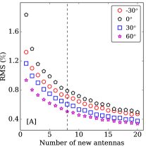
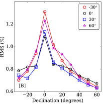
Figure 3: Results for the optimization for FWHM $=0.5$ km, i.e. $b_{\rm max}=1.0$ km. [A] The Residual RMS plotted versus the number of new antennas, for $\delta=-30^{\circ}$, $0^{\circ}$, $+30^{\circ}$, and $+60^{\circ}$; the dashed vertical line indicates 8 antennas, beyond which the decline in Residual RMS with added antennas flattens out. [B] The Residual RMS for the best configurations for the four declinations with 8 new antennas plotted against declination. The configuration with $\delta=+30^{\circ}$ yields the best overall performance. [C] The locations of the new antennas, indicated by red stars, and of the existing GMRT antennas, indicated by solid black circles. See text for discussion.

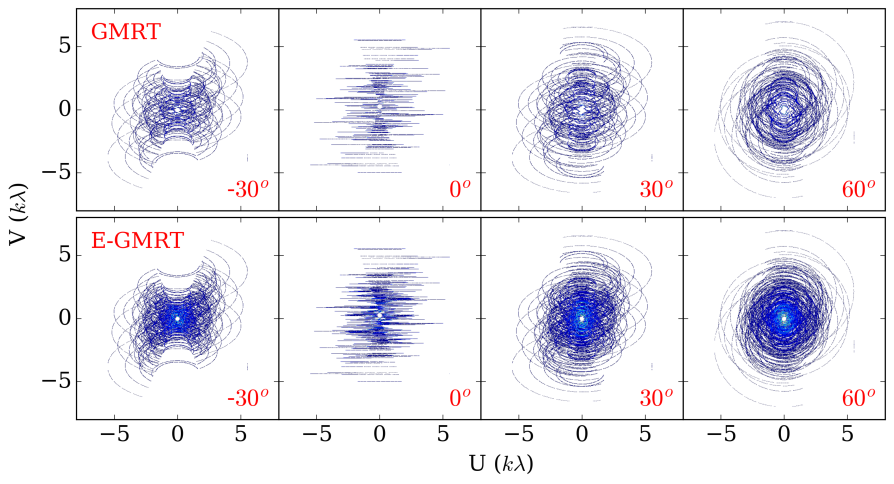
Figure 4: A comparison between the U-V coverage of the uGMRT and the EGMRT, for baselines out to 1 km (i.e. for the EGMRT optimization for FWHM $=0.5$ km), for declinations $\delta=-30^{\circ}$, $0^{\circ}$, $+30^{\circ}$, and $+60^{\circ}$, for a full-synthesis observing run at 1.2 GHz. The U-V coverage has been computed using a single channel.

Our optimization strategy was based on the fact that it is desirable for imaging of complex fields (e.g. the Galactic plane) to have a well-behaved synthesized beam over a range of angular resolutions, and especially at the shorter baselines which are sensitive to extended radio emission on a range of angular scales. We hence adopted an “inside-out” optimization strategy, first optimizing the array configuration for the shortest baselines (FWHM of the 2-D Gaussian in the U-V plane of 0.5 km), then for short baselines (FWHM $=1.7$ km), then for intermediate baselines (FWHM $=5$ km), then for longer baselines (FWHM $=15$ km), and finally for the full array (FWHM $=25$ km). In other words, instead of optimizing the full EGMRT configuration at once, we optimized the array configuration in steps, in which the optimization at each step is carried out for a given maximum baseline. At the next step, the antenna locations optimized in the previous step are kept fixed, and only the new added antenna locations are allowed to vary in the optimization. The resulting array would thus have a well-behaved synthesized beam over a range of angular resolutions, and not merely at the highest angular resolution.

We further note that the above FWHM’s of the 2-D Gaussian distributions of the U-V coverage were not set to be equal to the longest baseline of the array whose configuration was being optimized. This was done because there are, of course, baselines beyond the FWHM that contribute to the 2-D Gaussian U-V distribution. We hence allowed longest baselines of $b_{\rm max}\approx 1$ km for FWHM $=0.5$ km, of $\approx 5$ km for FWHM $\approx 1.7$ km, of $\approx 15$ km for FWHM $\approx 5$ km, of $\approx 25$ km for FWHM $\approx 15$ km, of $\approx 50$ km for FWHM $\approx 25$ km.

As mentioned above, the optimizations out to $b_{\rm max}=5.0$ km (i.e. FWHM $\approx 1.7$ km) were carried out using the random sampling approach, as the total number of possible antenna locations is relatively small. Since the GMRT antennas have a diameter of 45 m, we divided the possible antenna locations (including any land constraints) into cells of size $60$ m $\times 60$ m (smaller cells would have meant large shadowing of antennas by each other; note that our optimization approach does not include a penalty for shadowing). For a region of size $\approx 1.7$ km $\times 1.7$ km, this meant $\approx 800$ possible locations for the new antennas, after including the land constraints. This could be handled in reasonable computing time via random sampling, estimating the Residual RMS for $10^{4}$ random antenna configurations, and then choosing the configuration with the minimum Residual RMS. We hence chose to use random sampling for maximum baselines out to $b_{\rm max}=5$ km. We also verified that very similar antenna configurations were obtained using iAntConfig and random-sampling for the most compact configuration, with FWHM $\approx 0.5$ km. For $b_{\rm max}\gg 5$ km, it was clear that random sampling would not provide sufficient coverage of the possible antenna configurations in reasonable computing time. For the optimization for $b_{\rm max}\geq 15$ km (i.e. FWHM $\gtrsim 5$ km), we hence used the tomographic projection approach (de Villiers, 2007).

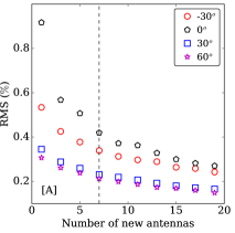
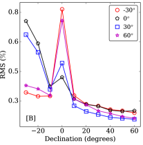
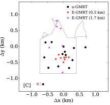
Figure 5: Results for the optimization for FWHM $=1.7$ km, i.e. $b_{\rm max}=5$ km. [A] The Residual RMS plotted versus the number of new antennas, for $\delta=-30^{\circ}$, $0^{\circ}$, $+30^{\circ}$, and $+60^{\circ}$; the dashed vertical line indicates 7 antennas, beyond which the decline in Residual RMS with added antennas flattens out. [B] The Residual RMS for the best configurations for the four declinations with 7 new antennas plotted against declination. The configuration with $\delta=+30^{\circ}$ yields the best overall performance. [C] The locations of the GMRT antennas are indicated by solid black circles, of the 8 new antennas obtained in the FWHM $=0.5$ km optimization by red stars, and of the 7 new antennas obtained here by magenta stars. See text for discussion.

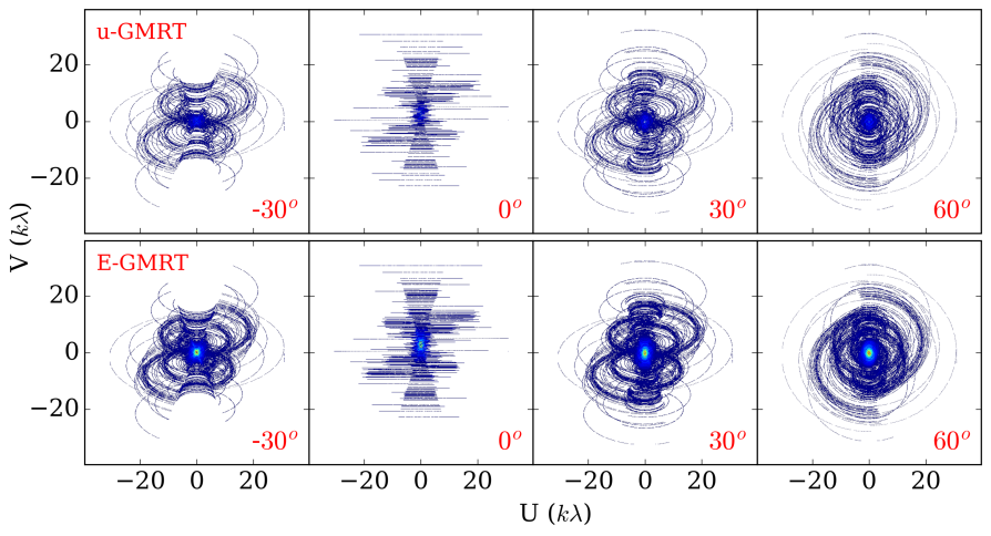
Figure 6: A comparison between the single-channel U-V coverage of the GMRT and the EGMRT, for baselines out to 5 km (i.e. for the EGMRT optimization for FWHM $=1.7$ km), for the four declinations, for a full synthesis observing run at 1.2 GHz.

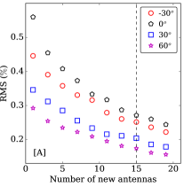
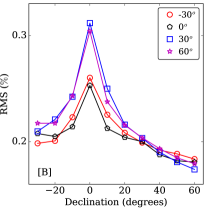
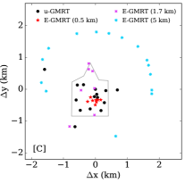
Figure 7: Results for the optimization for FWHM $=5$ km, i.e. $b_{\rm max}=15$ km. [A] The Residual RMS plotted versus the number of new antennas, for $\delta=-30^{\circ}$, $0^{\circ}$, $+30^{\circ}$, and $+60^{\circ}$; the dashed vertical line indicates 15 antennas, beyond which the decline in Residual RMS with added antennas slows down. [B] The Residual RMS for the best configurations for the four declinations with 15 new antennas plotted against declination. The configuration with $\delta=0^{\circ}$ yields the best overall performance. [C] The locations of the GMRT antennas are indicated by solid black circles, of the 8 new antennas obtained in the FWHM $=0.5$ km optimization by red stars, of the 7 new antennas obtained in the FWHM $=1.7$ km optimization by magenta stars, and of the 15 new antennas obtained here by blue stars. See text for discussion.

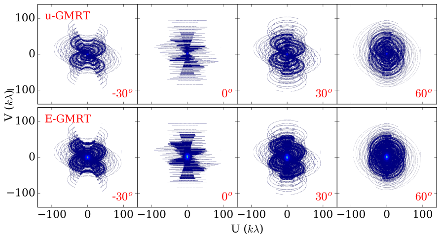
Figure 8: A comparison between the single-channel U-V coverage of the GMRT and the EGMRT, for a maximum baseline of 15 km (i.e. for the EGMRT optimization for FWHM $=5.0$ km), for the four declinations, for a full synthesis observing run at 1.2 GHz.

4.3.1 Optimization for FWHM $=0.5$ km, i.e. $b_{\rm max}=1.0$ km

The first step of our optimization is for FWHM $=0.5$ km. Here, as noted above, we used both the random sampling and tomographic projection methods, and obtained very similar results from the two approaches. Both approaches are described in detail below. We finally used the results from the tomographic projection method.

The spatial density of the existing GMRT antennas is maximum in the central square, with baselines of $\lesssim 1$ km. Hence, the optimization for FWHM $=0.5$ km, following both approaches, was carried out by restricting the EGMRT antenna locations to lie within the central square. Further, we included only the 14 GMRT central square antennas as “fixed” antennas in the optimization.

In the tomographic projection method, beginning with the above fixed GMRT antennas, we add N new antennas to the array, starting with ${\rm N}=1$, and increasing the number of new antennas by one at each iteration. For each value of N, we carried out the tomographic projection optimization for 100 random initial conditions for the new antenna locations, and evaluated the final Residual RMS for each of the 100 realizations. We then chose the realization with the lowest Residual RMS as the optimal configuration for the N new antennas. This minimum Residual RMS was saved, along with the locations of the new antennas, and the process repeated for (N+1) new antennas. The Residual RMS initially declines steeply with each new added antenna, as the U-V coverage approaches a 2-D Gaussian U-V distribution. However, beyond some number of new antennas, there is no significant decrease in the Residual RMS, i.e. improvement in the U-V coverage, on adding more antennas. We fixed the number of new antennas to the number above which the Residual RMS does not change by more than $\approx 10$% with the addition of further new antennas.

In the random-sampling method, we again add N new antennas to the array, starting with ${\rm N}=1$, and increasing the number of new antennas by one at each iteration. However, here we randomly assign the new antennas to available cells in the GMRT central square, keeping the locations of the existing GMRT antennas fixed. We then evaluate the Residual RMS for the configuration, comparing the U-V coverage of the configuration with the “ideal” 2-D Gaussian of FWHM $=0.5$ km. We carry out this random assignment process $10^{4}$ times for each value of N, and determine the minimum Residual RMS for the $10^{4}$ evaluated configurations. This minimum Residual RMS is then stored, again along with the locations of the new antennas, and the process is repeated, by adding (N+1) antennas. We find a pattern similar to that seen in the tomographic projection approach, i.e. that the Residual RMS initially declines steeply with each added antenna, but, beyond some number of new antennas, does not decrease significantly on adding more antennas. Again, the number of new antennas is then fixed to the number above which the Residual RMS does not change by more than $\approx 10$% with the addition of further new antennas.

As noted earlier, the above process was carried out independently for four declinations, $\delta=-30^{\circ}$, $+30^{\circ}$ and $+60^{\circ}$. Fig. 3[A] shows the Residual RMS plotted against the number of antennas for the four different declinations, with the results obtained via the tomographic projection method. The dashed vertical line indicates 8 added antennas, beyond which the Residual RMS improves only slowly with additional antennas (for all four declinations).

Following this, the Residual RMS obtained from the four “best” configurations with 8 EGMRT antennas (from each of the four declinations) was then evaluated as a function of declination, over the declination range $-30^{\circ}$ to $+60^{\circ}$, to identify the best configuration for all declinations. Fig. 3[B] shows the Residual RMS plotted versus declination for the four different configurations, labelled by the declination at which the configuration was optimized. For the case of FWHM $=0.5$ km, we find that the best results over the full declination range were obtained from the configuration optimized for $\delta=+30^{\circ}$. This array configuration is shown in Fig. 3[C], with the 14 GMRT central square antennas shown as solid black circles and the 8 new EGMRT antennas shown as red stars.

Finally, Fig. 4 compares the U-V coverage obtained in a full-synthesis observing run with the 14 GMRT central square antennas with that obtained with the EGMRT array with 8 new antennas, for $\delta=-30^{\circ}$, $0^{\circ}$, $+30^{\circ}$, and $+60^{\circ}$. It is clear that the EGMRT array would yield significantly better U-V coverage than that of the present GMRT for all declinations; similar results are obtained for snapshot observations.

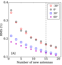
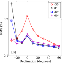
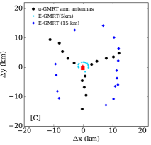
Figure 9: Results for the optimization for FWHM $=15$ km, i.e. $b_{\rm max}=25$ km. [A] The Residual RMS plotted versus the number of new antennas, for $\delta=-30^{\circ}$, $0^{\circ}$, $+30^{\circ}$, and $+60^{\circ}$; the dashed vertical line indicates 15 antennas, beyond which the decline in Residual RMS with added antennas slows down. [B] The Residual RMS for the best configurations for the four declinations with 15 new antennas plotted against declination. The configuration with $\delta=+60^{\circ}$ yields the best overall performance. [C] The locations of the GMRT antennas are indicated by solid black circles, of the 15 new antennas obtained in the FWHM $=5.0$ km optimization by cyan stars, and of the 15 new antennas obtained here by blue diamonds. See text for discussion.

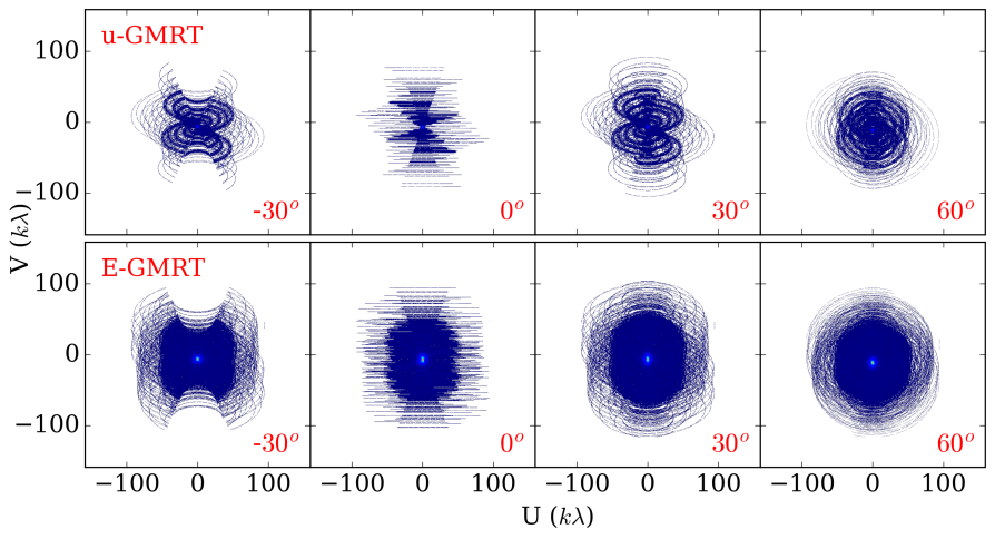
Figure 10: A comparison between the single-channel U-V coverage of the GMRT and the EGMRT, for baselines out to 25 km (i.e. for the EGMRT optimization for FWHM $=15$ km), for the four declinations, for a full synthesis observing run at 1.2 GHz.

4.3.2 Optimization for FWHM $=1.7$ km, i.e. $b_{\rm max}=5.0$ km

For the next step, the optimization for FWHM $=1.7$ km, we included all existing GMRT antennas with baselines out to 5 km (twenty antennas in all), as well as the 8 new EGMRT antenna locations obtained above, as fixed antennas. The new antenna locations were constrained to be on land either currently owned by the GMRT or on land that might be acquired for the expansion. We note that this implied significant constraints on the allowed antenna locations, and hence, that better results (i.e. a lower Residual RMS) were obtained with the random-sampling method than with the tomographic projection method (which applies land constraints at the end of the optimization in an ad hoc manner). We hence used the random-sampling approach to identify the new antenna locations for $b_{\rm max}=5.0$ km, following the procedure described in Section 4.3.1, except that new antennas were added in steps of two, rather than one, to reduce the computational requirements.

Fig. 5[A] shows the Residual RMS plotted against the number of antennas for the four different declinations; the dashed vertical line is for 7 new antennas, above which we do not find a significant improvement in the Residual RMS on adding further antennas. Fig. 5[B] shows the Residual RMS plotted against declination for the best configurations obtained with 7 new antennas for the four different declinations; we find that the best overall performance is obtained for the configuration for $\delta=-30^{\circ}$. This is shown in Fig. 5[C], with GMRT antennas shown as solid black circles, EGMRT antennas obtained from the FWHM $=0.5$ km optimization as red stars, and EGMRT antennas obtained from the FWHM $=1.7$ km optimization as magenta stars. Fig. 6 shows a comparison between the single-channel U-V coverage of the GMRT array with baselines out to $b_{\rm max}=5.0$ km and the EGMRT array (with 20 GMRT antennas and 15 new antennas), for a full-synthesis observing run and the different declinations. Again, it is clear that significantly better U-V coverage is obtained with the EGMRT array.

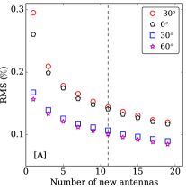
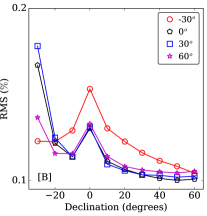
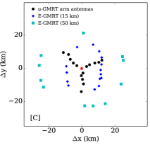
Figure 11: Results for the optimization for FWHM $=25$ km, i.e. $b_{\rm max}=50$ km. [A] The Residual RMS plotted versus the number of new antennas, for $\delta=-30^{\circ}$, $0^{\circ}$, $+30^{\circ}$, and $+60^{\circ}$; the dashed vertical line indicates 11 antennas, beyond which the decline in Residual RMS with added antennas slows down. [B] The Residual RMS for the best configurations for the four declinations with 11 new antennas plotted against declination. The configuration with $\delta=+60^{\circ}$ yields the best overall performance. [C] The locations of the GMRT antennas are indicated by solid black circles, of the 15 new antennas obtained in the FWHM $=15.0$ km optimization by blue diamonds, and of the 11 new antennas obtained here by cyan squares. See text for discussion.

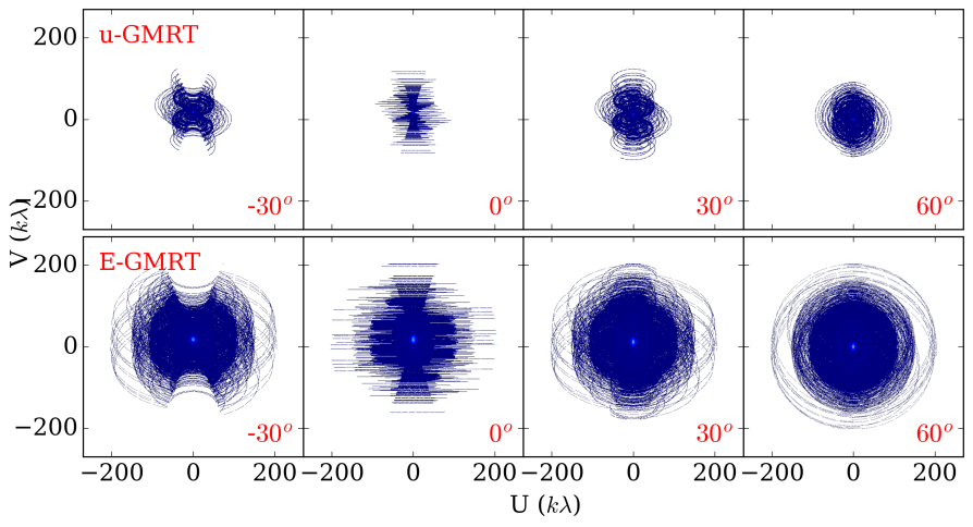
Figure 12: A comparison between the single-channel U-V coverage of the full GMRT and the full EGMRT, i.e. with baselines out to 25 km for the GMRT and to 50 km for the EGMRT for the four declinations, for a full-synthesis observing run at 1.2 GHz.

4.3.3 Optimization for FWHM $=5.0$ km, i.e. $b_{\rm max}=15.0$ km

The next step, the optimization for FWHM $=5.0$ km, included all the current GMRT antennas as fixed antennas, as each GMRT antenna yields a number of baselines of length $<15$ km. We also included the 15 EGMRT antennas obtained from the earlier two optimizations as fixed antennas in the optimization. The optimization used the tomographic projection approach and did not include any land constraints.

Fig. 7[A] shows the Residual RMS plotted against the number of antennas for $\delta=-30^{\circ}$, $0^{\circ}$, $+30^{\circ}$, and $+60^{\circ}$; the dashed vertical line is for 15 new antennas, above which the improvement in Residual RMS with added antennas flattens. Fig. 7[B] shows the Residual RMS plotted against declination for the best configurations obtained with 15 new antennas for each of the four declinations. The best overall performance is obtained for the configuration with $\delta=0^{\circ}$, shown in Fig. 7[C]. Fig. 8 shows a comparison between the U-V coverage of the GMRT array with baselines out to $b_{\rm max}=15.0$ km and the best EGMRT array (with 20 GMRT antennas and 30 new antennas), for the four declinations, and a full-synthesis run.

4.3.4 Optimization for FWHM $=15.0$ km, i.e. $b_{\rm max}=25.0$ km

Next, we fixed the locations of the 30 new antennas along with the 30 existing GMRT antennas, and carried out the optimization, using tomographic projection, for FWHM $=15$ km, with $b_{\rm max}=25.0$ km. Again, no land constraints were used in the optimization. Fig. 9[A] shows the derived Residual RMS plotted versus the number of added antennas for the four different declinations; the dashed vertical line is at 15 new antennas, where the decline in the Residual RMS with new antennas slows down. Fig. 9[B] shows the Residual RMS plotted versus declination for the best configurations with 15 new antennas; we find that the configuration with $\delta=+60^{\circ}$, shown in Fig. 9[C] gives the best overall performance. Fig. 10 compares the U-V coverage of the GMRT array with baselines out to $b_{\rm max}=25.0$ km and the best above EGMRT array (with 30 GMRT antennas and 45 new antennas), for a full-synthesis observing run, for the different declinations.

4.3.5 Optimization for FWHM $=25.0$ km, i.e. $b_{\rm max}=50.0$ km

Finally, we carried out the optimization for FWHM $=25.0$ km, fixing the locations of the 30 GMRT antennas and the 45 new EGMRT antennas, and again using the tomographic projection approach without land constraints, with $b_{\rm max}=50$ km. Fig. 11[A] shows the Residual RMS plotted versus the added number of antennas for the four different declinations; the dashed vertical line is at 11 new antennas, beyond which the decline in Residual RMS with added antennas appears to flatten out. Fig. 11[B] shows the Residual RMS of the four best configurations obtained with 11 new antennas plotted versus declination; the configuration obtained from $\delta=+60^{\circ}$, shown in Fig. 11[C], yields the best overall performance. The U-V coverage of this array is shown in Fig. 12 for a full-synthesis run, for the four different declinations. We note that the GMRT array only provides baselines out to $\approx 25$ km. With $b_{\rm max}\approx 50$ km, the EGMRT array would have a synthesized beam smaller by a factor of $\approx 2$, and would hence have a confusion noise lower by a factor of $\approx 10$ than that of the uGMRT at the same observing frequency.

5 Discussion

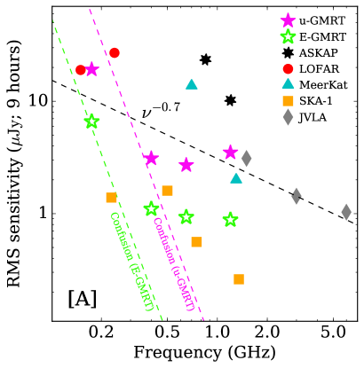
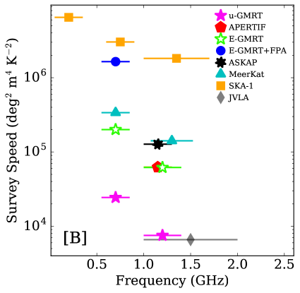
Figure 13: [A] Left panel: The $1\sigma$ continuum noise of the EGMRT compared with that of the other radio interferometers of Fig. 2 (the uGMRT, the JVLA, LOFAR, MeerKAT, ASKAP, and the SKA-1) for a 9-hour full-synthesis integration. The green and magenta dashed lines show the $1\sigma$ confusion noise for, respectively, the EGMRT and the uGMRT, at the different observing frequencies. It is clear that source confusion will be a limiting factor for the EGMRT only in its lowest frequency band ($125-250$ MHz), where the sensitivity is likely to anyway be limited by systematic effects, rather than thermal noise. Note that the $1\sigma$ continuum noise values for ASKAP and MeerKAT include confusion noise, also extrapolated from Condon et al. (2012). [B] Right panel: The survey speed figure of merit, in deg.² m⁴ K^-2 (e.g. Dewdney et al., 2015), of the EGMRT compared with that of other present or planned radio interferometers. For the EGMRT, we have considered two possibilities: the open green stars (“EGMRT”) refer to single-pixel feeds on all 86 antennas, while the solid blue circles (“EGMRT+FPA”) assume FPAs covering $550-850$ MHz installed on the 45 antennas within $\approx 2.5$ km of the central square.

We thus find that adding 56 new antennas to the GMRT array, 30 antennas at distances $\lesssim 2.5$ km from the GMRT central square, and 26 antennas more distant from the central square (at distances $\approx 7.5-25$ km), would significantly improve the U-V coverage of the array. The resulting baselines would, for declinations $\delta\approx-30^{\circ}-+60^{\circ}$, yield a U-V coverage close to a 2-D Gaussian distribution with FWHM’s of $\approx 0.5$ km, $\approx 1.7$ km, $\approx 5.0$ km, $\approx 15$ km, and $\approx 25$ km, depending on the maximum baseline used in the imaging process. The longitudes and latitudes of the new EGMRT antennas are listed in Table 1 in the Appendix, where each pair of longitude and latitude columns refers to antenna locations obtained in optimizations for increasing FWHM’s ($0.5-25$ km) of the U-V coverage.

Fig. 13[A] compares the continuum sensitivity of the proposed EGMRT array to that of the other radio interferometers of Fig. 2, with the EGMRT values shown as open green stars. We assume that the EGMRT will have 86 dishes of 45-m diameter, with baselines out to $\approx 50$ km, and that the instantaneous correlated bandwidth and the receiver sensitivity will be the same as that of the uGMRT. It is clear that the EGMRT point-source sensitivity would be similar to that of the SKA-1 over $\approx 0.3-1.4$ GHz, and would be significantly better than that of any other radio telescope over its entire operating frequency range.

Fig. 13[B] compares the survey speed of the proposed EGMRT with present and proposed radio interferometers at frequencies $\lesssim 2$ GHz. For this comparison, we have used the survey speed figure of merit of Dewdney et al. (2015), defined as $\rm(A_{eff}/T_{sys})^{2}\Omega$ (in deg.² m⁴ K^-4), where $\rm A_{eff}$ is the effective area of the array, $\rm T_{sys}$ is its system temperature, and $\Omega$ is its instantaneous field-of-view. Two configurations are shown for the EGMRT, the first (“EGMRT+FPA”) with FPAs covering $550-850$ MHz installed on the 45 antennas within 5 km baselines, and the second (“EGMRT”) with single-pixel feeds on all 86 antennas. It is clear that the survey speed of the first EGMRT configuration, with FPAs at $550-850$ MHz installed on 45 antennas, would be better than that of all present radio interferometers, and comparable to that of the SKA-1 in the same frequency band.

6 Summary

We have discussed three possible expansions of the GMRT to improve its surface brightness sensitivity, field of view (and, hence, survey speed), and confusion limit, and to retain its status as the premier low-frequency ($\lesssim 1$ GHz) radio interferometer beyond the next decade. The three expansions involve adding antennas at short baselines (for surface brightness sensitivity) or on long baselines (to reduce the confusion noise), or replacing the GMRT single-pixel feeds with FPAs to significantly increase the field of view. The primary science drivers of the three expansions are very different: adding FPAs would enable searches for Hi 21 cm emission from high-$z$ galaxies and wide-field pulsar and continuum surveys, the short-baseline expansion would significantly improve the GMRT’s capabilities for the mapping of extended radio emission in the Galactic Plane, in galaxy clusters, etc., while the long-baseline expansion would lower the confusion limit, allowing deep extra-galactic continuum studies. These will be discussed in detail in future science papers. To retain the multi-science capabilities of the GMRT, we propose that it would be best to not focus on a single expansion strategy, but to add antennas on both short and long baselines, and to also add FPAs on a subset of the antennas, on baselines $\lesssim 2.5$ km from the GMRT central square. Such a strategy would retain scientific flexibility, while significantly improving the capabilities of the expanded array for all the above science goals.

To achieve the above goal, we then identified the optimal locations for the new antennas of the proposed array, following an inside-out approach aimed at obtaining a well-behaved synthesized beam over a wide range of angular scales. While the final antenna locations of the EGMRT, especially on the long baselines, will depend on practical constraints, including land availability, optical fibre connectivity, roads, etc., the present configuration provides a benchmark array, relative to which one can evaluate the final EGMRT configuration. The array optimization was carried out by choosing antenna locations so as to obtain a U-V coverage as close as possible to a 2-D circular Gaussian distribution (which would yield a 2-D Gaussian synthesized beam), with different FWHM’s (0.5 km, 1.7 km, 5 km, 15 km, and 25 km), and for a wide range of declinations ($-30^{\circ}$ to $+60^{\circ}$). The optimization of antenna locations was carried out using two strategies, random-sampling for antennas located close to the GMRT central square, i.e. for FWHM’s $\leq 1.7$ km, and tomographic projection for FWHM’s $\geq 5$ km. We find that the requirement that the U-V coverage be close to a 2-D circular Gaussian can be met by adding $8$ antennas within the central $\approx 0.5$ km region of the GMRT central square, $7$ antennas at distances $\approx 0.5-1$ km from the central square, $15$ antennas $\approx 1-2.5$ km from the central square, $15$ antennas $\approx 7.5$ km from the central square and $11$ antennas $\approx 25$ km from the central square. The 30 new EGMRT antennas within $\approx 2.5$ km of the central square would contribute significantly towards improving the surface brightness sensitivity, as well as the sensitivity for pulsar surveys and searches for redshifted Hi 21 cm emission, while the 11 antennas on baselines $\gtrsim 25$ km would contribute to improving the confusion limit for extragalactic continuum studies. We further propose to install FPAs on the new EGMRT and existing GMRT antennas within a $\approx 5$ km region around the GMRT central square, to achieve a large field of view for this group of 45 antennas, significantly improving the survey speed of the array.

Finally, we compared the sensitivity and survey speed of the proposed new EGMRT array, with 56 new antennas, to that of existing and planned radio interferometers. We find that the point-source sensitivity of the EGMRT would be similar to that of the proposed SKA-1 at frequencies $300-1000$ MHz, and significantly better than that of all other existing and planned interferometers at frequencies $\lesssim 1.4$ GHz. Similarly, the survey speed of the EGMRT sub-array equipped with FPAs would be comparable to that of the SKA-1 at a similar frequency, and higher than that of any other existing or planned radio interferometer. The proposed expansions would thus allow the GMRT to retain its status as the premier low-frequency radio interferometer in the world well beyond the next decade, and into the SKA era.

Appendix A

Table 1: The coordinates of the new EGMRT antennas

0.5 km		1.7 km		5 km		15 km		50 km
Long. (∘)	Lat. (∘)	Long. (∘)	Lat. (∘)	Long. (∘)	Lat. (∘)	Long. (∘)	Lat. (∘)	Long. (∘)	Lat. (∘)
74.0507725	19.0900447	74.0463238	19.0928289	74.0664129	19.0999286	73.9609521	19.1032398	74.0664124	18.8880061
74.0509136	19.0894700	74.0429033	19.0825301	74.0673838	19.0928796	74.1478274	18.9959265	74.2835108	19.1559832
74.0497636	19.0898942	74.0486044	19.0987914	74.0366723	19.1047456	73.9672950	19.0201074	74.1844691	18.8994765
74.0482780	19.0896067	74.0486044	19.1004175	74.0348558	19.1015569	74.0227518	19.2076507	74.2757907	19.0063713
74.0505633	19.0886720	74.0503149	19.0933710	74.0345159	19.0949776	74.1580258	19.0830605	74.0590555	19.2845531
74.0513364	19.0901220	74.0503149	19.0857825	74.0546174	19.1089636	73.9727482	18.9983853	73.8157773	19.1618540
74.0491589	19.0908299	74.0497447	19.0982494	74.0508886	19.1093734	74.1629440	19.1133690	73.8299016	18.9894072
74.0521847	19.0900995			74.0585228	19.1077731	74.1620281	19.0395763	74.2884355	19.1360591
				74.0673717	19.0918209	74.1147037	19.2212894	73.8146510	19.0262421
				74.0450750	19.1089053	74.1235203	18.9773132	74.1148953	18.8873737
				74.0669867	19.0973430	74.1532751	19.0351790	73.8052941	19.1077472
				74.0659674	19.1013593	74.1588607	19.0598107
				74.0359408	19.0925731	74.1496416	19.1847213
				74.0566546	19.0797704	74.1642385	19.1511805
				74.0632511	19.1052599	73.9635819	19.0694059

References

- Aditya, Kanekar & Kurapati (2016) Aditya J. N. H. S., Kanekar N., Kurapati S., 2016, MNRAS, 455, 4000
- Anantharamaiah et al. (1991) Anantharamaiah K. R., Pedlar A., Ekers R. D., Goss W. M., 1991, MNRAS, 249, 262
- Bagchi et al. (2007) Bagchi J., Gopal-Krishna, Krause M., Joshi S., 2007, ApJL, 670, L85
- Bagchi et al. (2014) Bagchi J. et al., 2014, ApJ, 788, 174
- Begum et al. (2006) Begum A., Chengalur J. N., Karachentsev I. D., Kaisin S. S., Sharina M. E., 2006, MNRAS, 365, 1220
- Begum et al. (2008) Begum A., Chengalur J. N., Karachentsev I. D., Sharina M. E., Kaisin S. S., 2008, MNRAS, 386, 1667
- Bhatnagar (2000) Bhatnagar S., 2000, MNRAS, 317, 453
- Bhattacharyya et al. (2016) Bhattacharyya B. et al., 2016, ApJ, 817, 130
- Bhattacharyya et al. (2013) Bhattacharyya B. et al., 2013, ApJL, 773, L12
- Boone (2001) Boone F., 2001, A&A, 377, 368
- Booth et al. (2009) Booth R. S., de Blok W. J. G., Jonas J. L., Fanaroff B., 2009, ArXiv e-prints
- Bouwens et al. (2014) Bouwens R. J., et al., 2014, Ap, 795
- Boyle & Chime/Frb Collaboration (2018) Boyle P. C., Chime/Frb Collaboration, 2018, The Astronomer’s Telegram, 11901
- Brunetti et al. (2008) Brunetti G. et al., 2008, Nature, 455, 944
- Brunetti et al. (2007) Brunetti G., Venturi T., Dallacasa D., Cassano R., Dolag K., Giacintucci S., Setti G., 2007, ApJL, 670, L5
- Buch et al. (2016) Buch K. D., Bhatporia S., Gupta Y., Nalawade S., Chowdhury A., Naik K., Aggarwal K., Ajithkumar B., 2016, Jour. Astr. Instr., 5, 1641018
- Chandra & Kanekar (2017) Chandra P., Kanekar N., 2017, ApJ, 846, 111
- Chandra, Ray & Bhatnagar (2004) Chandra P., Ray A., Bhatnagar S., 2004, ApJ, 612, 974
- Chengalur & Kanekar (2003) Chengalur J. N., Kanekar N., 2003, Phys. Rev. Lett., 91, 241302
- Chengalur & Kanekar (2003) Chengalur J. N., Kanekar N., 2003, A&A, 403, L43
- Chippendale et al. (2016) Chippendale A. P., Beresford R. J., Deng X., Leach M., Reynolds J. E., Kramer M., Tzioumis T., 2016, in 2016 International Conference on Electromagnetics in Advanced Applications (ICEAA), Cairns, QLD, p. 909-912, p. 909
- Condon et al. (2012) Condon J. J. et al., 2012, ApJ, 758, 23
- de Villiers (2007) de Villiers M., 2007, A&A, 469, 793
- DeBoer et al. (2009) DeBoer D. R. et al., 2009, IEEE Proceedings, 97, 1507
- Deo & Kale (2017) Deo D. K., Kale R., 2017, Exp. Astr., 44, 165
- Dewdney et al. (2015) Dewdney P. E., Turner W., Braun R., Santander-Vela J., Tan G.-H., 2015, SKA Report SKA-TEL-SKO-0000308
- Freire et al. (2004) Freire P. C., Gupta Y., Ransom S. M., Ishwara-Chandra C. H., 2004, ApJL, 606, L53
- Gangadhara & Gupta (2001) Gangadhara R. T., Gupta Y., 2001, ApJ, 555, 31
- Garn et al. (2007) Garn T., Green D. A., Hales S. E. G., Riley J. M., Alexander P., 2007, MNRAS, 376, 1251
- Geller et al. (2000) Geller R. M., Sault R. J., Antonucci R., Killeen N. E. B., Ekers R., Desai K., Whysong D., 2000, ApJ, 539, 73
- Giacintucci et al. (2011) Giacintucci S. et al., 2011, ApJ, 732, 95
- Gupta et al. (2006) Gupta N., Salter C. J., Saikia D. J., Ghosh T., Jeyakumar S., 2006, MNRAS, 373, 972
- Gupta et al. (2017) Gupta Y. et al., 2017, Curr. Sci., 113, 707
- Hermsen et al. (2013) Hermsen W., et al., 2013, Science, 339, 436
- Hopkins & Beacom (2006) Hopkins A. M., Beacom J. F., 2006, ApJ, 651, 142
- Hyman et al. (2009) Hyman S. D., Wijnands R., Lazio T. J. W., Pal S., Starling R., Kassim N. E., Ray P. S., 2009, ApJ, 696, 280
- Ibar et al. (2009) Ibar E., Ivison R. J., Biggs A. D., Lal D. V., Best P. N., Green D. A., 2009, MNRAS, 397, 281
- Intema et al. (2017) Intema H. T., Jagannathan P., Mooley K. P., Frail D. A., 2017, A&A, 598, A78
- Ishwara-Chandra, Dwarakanath & Anantharamaiah (2003) Ishwara-Chandra C. H., Dwarakanath K. S., Anantharamaiah K. R., 2003, JA&A, 24, 37
- Ishwara-Chandra et al. (2010) Ishwara-Chandra C. H., Sirothia S. K., Wadadekar Y., Pal S., Windhorst R., 2010, MNRAS, 405, 436
- Johnston et al. (2008) Johnston S., et al., 2008, Ex. A., 22, 151
- Kale et al. (2015) Kale R. et al., 2015, A&A, 579, A92
- Kanekar (2014) Kanekar N., 2014, ApJL, 797, L20
- Kanekar, Braun & Roy (2011) Kanekar N., Braun R., Roy N., 2011, ApJ, 737, L33
- Kanekar & Chengalur (2002) Kanekar N., Chengalur J. N., 2002, A&A, 381, L73
- Kanekar & Chengalur (2003) Kanekar N., Chengalur J. N., 2003, A&A, 399, 857
- Kanekar et al. (2009) Kanekar N., Prochaska J. X., Ellison S. L., Chengalur J. N., 2009, MNRAS, 396, 385
- Kanekar et al. (2010) Kanekar N., Prochaska J. X., Ellison S. L., Chengalur J. N., 2010, ApJ, 712, L148
- Kanekar et al. (2014) Kanekar N. et al., 2014, MNRAS, 438, 2131
- Kanekar, Sethi & Dwarakanath (2016) Kanekar N., Sethi S., Dwarakanath K. S., 2016, ApJL, 818, L28
- Keto (1997) Keto E., 1997, ApJ, 475, 843
- Lah et al. (2007) Lah P. et al., 2007, MNRAS, 376, 1357
- Lah et al. (2009) Lah P. et al., 2009, MNRAS, 399, 1447
- Lal & Rao (2007) Lal D. V., Rao A. P., 2007, MNRAS, 374, 1085
- LaRosa et al. (2000) LaRosa T. N., Kassim N. E., Lazio T. J. W., Hyman S. D., 2000, AJ, 119, 207
- Lorimer et al. (2007) Lorimer D. R., Bailes M., McLaughlin M. A., Narkevic D. J., Crawford F., 2007, Science, 318, 777
- Mauch et al. (2013) Mauch T., Klöckner H.-R., Rawlings S., Jarvis M., Hardcastle M. J., Obreschkow D., Saikia D. J., Thompson M. A., 2013, MNRAS, 435, 650
- McCready, Pawsey & Payne-Scott (1947) McCready L. L., Pawsey J. L., Payne-Scott R., 1947, Proc. Roy. Soc. London Ser. A, 190, 357
- Mills & Slee (1957) Mills B. Y., Slee O. B., 1957, Aust. Jour. Phys., 10, 162
- Mitchell & Condon (1985) Mitchell K. J., Condon J. J., 1985, AJ, 90, 1957
- Nord et al. (2004) Nord M. E., Lazio T. J. W., Kassim N. E., Hyman S. D., LaRosa T. N., Brogan C. L., Duric N., 2004, AJ, 128, 1646
- O’Brien (1953) O’Brien P. A., 1953, MNRAS, 113, 597
- Paciga et al. (2013) Paciga G. et al., 2013, MNRAS, 433, 639
- Paciga et al. (2011) Paciga G. et al., 2011, MNRAS, 413, 1174
- Perley et al. (2011) Perley R. A., Chandler C. J., Butler B. J., Wrobel J. M., 2011, ApJL, 739, L1
- Petroff et al. (2016) Petroff E. et al., 2016, PASA, 33, 045
- Rhee et al. (2016) Rhee J., Lah P., Chengalur J. N., Briggs F. H., Colless M., 2016, MNRAS, 460, 2675
- Roy (2018) Roy J., 2018, arXiv/1801.02826
- Roy et al. (2015) Roy J. et al., 2015, ApJL, 800, L12
- Roy, Kanekar & Chengalur (2013) Roy N., Kanekar N., Chengalur J. N., 2013, MNRAS, 436, 2366
- Roy (2013) Roy S., 2013, ApJ, 773, 67
- Roy et al. (2010) Roy S., Hyman S. D., Pal S., Lazio T. J. W., Ray P. S., Kassim N. E., 2010, ApJL, 712, L5
- Roy & Pramesh Rao (2004) Roy S., Pramesh Rao A., 2004, MNRAS, 349, L25
- Roychowdhury et al. (2010) Roychowdhury S., Chengalur J. N., Begum A., Karachentsev I. D., 2010, MNRAS, 404, L60
- Ryle (1952) Ryle M., 1952, Proceedings of the Royal Society of London Series A, 211, 351
- Scheuer (1957) Scheuer P. A. G., 1957, Proc. Cam. Phil. Soc., 53, 764
- Sebastian et al. (2018) Sebastian B., Ishwara-Chandra C. H., Joshi R., Wadadekar Y., 2018, MNRAS, 473, 4926
- Sholomitskii & Yaskovich (1990) Sholomitskii G. B., Yaskovich A. L., 1990, Sov. Astr. Lett., 16, 383
- Spitler et al. (2016) Spitler L. G. et al., 2016, Nature, 531, 202
- Swarup et al. (1991) Swarup G., Ananthakrishnan S., Kapahi V. K., Rao A. P., Subrahmanya C. R., Kulkarni V. K., 1991, Current Science, Vol. 60, NO.2/JAN25, P. 95, 1991, 60, 95
- Tamhane et al. (2015) Tamhane P., Wadadekar Y., Basu A., Singh V., Ishwara-Chandra C. H., Beelen A., Sirothia S., 2015, MNRAS, 453, 2438
- Taylor & Jagannathan (2016) Taylor A. R., Jagannathan P., 2016, MNRAS, 459, L36
- Thornton et al. (2013) Thornton D. et al., 2013, Science, 341, 53
- Tingay et al. (2013) Tingay S. J., et al., 2013, PASA, 30, e007
- Vadawale et al. (2003) Vadawale S. V., Rao A. R., Naik S., Yadav J. S., Ishwara-Chandra C. H., Pramesh Rao A., Pooley G. G., 2003, ApJ, 597, 1023
- van Ardenne et al. (2009) van Ardenne A., Bregman J. D., van Cappellen W. A., Kant G. W., de Vaate J. G. B., 2009, IEEE Proceedings, 97, 1531
- van Haarlem et al. (2013) van Haarlem M. P., et al., 2013, A&A, 556, A2
- van Weeren et al. (2017) van Weeren R. J. et al., 2017, Nature Astronomy, 1, 0005
- van Weeren et al. (2010) van Weeren R. J., Röttgering H. J. A., Brüggen M., Hoeft M., 2010, Science, 330, 347
- Venturi et al. (2007) Venturi T., Giacintucci S., Brunetti G., Cassano R., Bardelli S., Dallacasa D., Setti G., 2007, A&A, 463, 937
- Venturi et al. (2008) Venturi T., Giacintucci S., Dallacasa D., Cassano R., Brunetti G., Bardelli S., Setti G., 2008, A&A, 484, 327
- Verheijen et al. (2008) Verheijen M. A. W., Oosterloo T. A., van Cappellen W. A., Bakker L., Ivashina M. V., van der Hulst J. M., 2008, in AIPC Series, Vol. 1035, The Evolution of Galaxies Through the Neutral Hydrogen Window, Minchin R., Momjian E., eds., p. 265
- Wootten & Thompson (2009) Wootten A., Thompson A. R., 2009, IEEE Proceedings, 97, 1463
- Yusef-Zadeh, Hewitt & Cotton (2004) Yusef-Zadeh F., Hewitt J. W., Cotton W., 2004, ApJS, 155, 421