Mapping Informal Settlements in Developing Countries using Machine Learning and Low Resolution Multi-spectral Data

Abstract.

Informal settlements are home to the most socially and economically vulnerable people on the planet. In order to deliver effective economic and social aid, non-government organizations (NGOs), such as the United Nations Children’s Fund (UNICEF), require detailed maps of the locations of informal settlements. However, data regarding informal and formal settlements is primarily unavailable and if available is often incomplete. This is due, in part, to the cost and complexity of gathering data on a large scale. To address these challenges, we, in this work, provide three contributions. 1) A brand new machine learning data-set, purposely developed for informal settlement detection. 2) We show that it is possible to detect informal settlements using freely available low-resolution (LR) data, in contrast to previous studies that use very-high resolution (VHR) satellite and aerial imagery, something that is cost-prohibitive for NGOs. 3) We demonstrate two effective classification schemes on our curated data set, one that is cost-efficient for NGOs and another that is cost-prohibitive for NGOs, but has additional utility. We integrate these schemes into a semi-automated pipeline that converts either a LR or VHR satellite image into a binary map that encodes the locations of informal settlements.

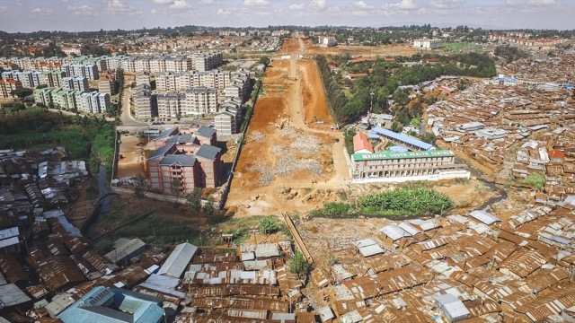
Figure 1. Divide between formal and informal settlements in Kibera, Nairobi. Copyright Unequal Scenes and Johnny Miller.

An example of informal settlements.

1. Introduction

The United Nations (UN) state that inhabitants of settlements that meet any of the following criteria are defined to be living in an informal settlement (United Nations, 2012):

1. Inhabitants have no security of tenure vis-à-vis the land or dwellings they inhabit, with modalities ranging from squatting to informal rental housing.

2. The neighborhoods usually lack, or are cut off from, basic services and city infrastructure.

3. The housing may not comply with current planning and building regulations, and is often situated in geographically and environmentally hazardous areas.

Slums, an example of informal settlements, are the most deprived and excluded form of informal settlements. They can be characterized by poverty and large agglomerations of dilapidated housing, located in the most hazardous urban land, near industries and dump sites, in swamps, degraded soils and flood-prone zones (Kohli et al., 2016). Slum dwellers are constantly exposed to eviction, disease and violence (Sclar et al., 2005), which stems from and leads to more severe economic and social constraints (Wekesa et al., 2011). Although informal settlements are well studied in the humanities and remote sensing communities (Fincher, 2003; Wekesa et al., 2011; United Nations, 2012; Huchzermeyer, 2006; Hofmann et al., 2008) in machine learning, only a small amount of research has been conducted on informal settlements, with all of that research using VHR and high resolution(HR) satellite imagery (Mahabir et al., 2018; Mboga et al., 2017; Varshney et al., 2015), a cost prohibitive option for many NGOs and governments of developing nations. In contrast, there is an abundance of freely available and globally accessible LR satellite imagery, provided by the European Space Agency (ESA), which provides updated imagery of the entire land mass of the Earth every 5 days (Wiatr et al., 2016; European Space Agency, 2018a, b). To the authors knowledge, no previous approaches have used LR imagery.

The ability to map and locate these settlements would give organizations such as UNICEF and other NGOs the ability to provide effective social and economic aid (Pais, 2002). This in turn would enable those communities to evolve in a sustainable way, allowing the people living in those environments to gain a much better quality of life addressing multiple of the UN sustainable development goals (United Nations, 2018). These goals aim to eliminate poverty, increase good health and well-being, provide quality education, clean water and sanitation, affordable and clean energy, sustainable work and economic growth, access to industry, innovation and infrastructure.

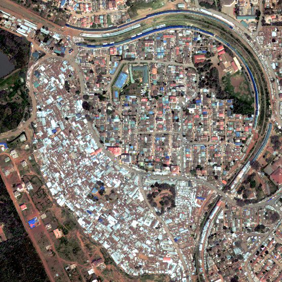
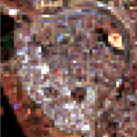
Figure 2. Two images of the same informal settlement in Kibera, representing the difference between VHR and LR imagery. Left: A DigitalGlobe 30cm VHR image. Right: The Sentinel-2 10m resolution image.

However, solving this problem is challenging due to several factors. 1) It requires collaboration among multiple parties: the NGOs, local government, the remote sensing and machine learning communities. 2) The locations and distribution of these informal settlements have yet to be mapped thoroughly on the ground or aerially, as the mapping demands dedicated human and financial resources. This often leads to partially completed, or completely un-annotated data-sets. 3) Informal settlements tend to grow sporadically (both in space and time), which adds an additional layer of complexity. 4) Even though we have access to satellite imagery for the entire globe, much of this raw data is not in a usable format for machine learning frameworks, making it difficult to extract actionable insights at scale (Xie et al., 2015). 5) There may be no local government structure in a particular settlement, which can inhibit our ability to gather data quickly. and make it difficult to extract good quality ground truth data, see Section 2.

In order to address these challenges, in this work we propose a semi-automated framework that takes a satellite image, directly extracted in its raw-user form and outputs a trained classifier that produces binary maps highlighting the locations of informal settlements.

Our first approach, the cost-effective approach, takes advantage of the pixel level contextual information by training a classifier to learn a unique spectral signal for informal settlements. When we require finer grained features, such as the roof size, or the density of the surrounding settlements to determine whether or not there exists an informal settlement, we demonstrate a second approach that uses a semantic segmentation neural network to extract these features, the cost-prohibitive solution. See Section 4.

To ensure that this work can be applied in the field, we have had an active partnership with UNICEF, to understand what we can do to facilitate their needs further and how we can facilitate the needs of other NGOs. Because of this, we focused on developing a system that will work in a computationally efficient and monetary effective manner. Our main approach runs efficiently on a laptop, or desktop CPU and is cost-effective as we only use freely available, openly accessible LR satellite imagery, rather than VHR imagery which can cost hundreds-of-thousands of dollars.

Within this paper we make the following contributions:

• We introduce and extensively validate two machine learning based approaches to detect and map informal settlements. One is cost-effective, the other is cost-prohibitive, but is required when contextual information is needed.

• We demonstrate for the first-time that informal settlements can be detected effectively using only freely and openly accessible LR satellite imagery.

• We release to the public two informal settlement benchmarks for LR and VHR satellite imagery, with accompanying ground truths.

• We provide all source code and models.

In Section 2 we provide details of the data used and the challenges involved in collecting it. In Section 3 we provide a condensed overview of related work and current approaches. In Section 4 we introduce details of our methodologies and present the results of our contributions in Section 5. Finally we conclude and present future work in Section 6.

2. Data Acquisition

In this work we use a combination of satellite imagery and on-the-ground measurements. However, to take advantage of machine learning frameworks we require an absolute ground truth, which facilitates robust training and validation. Ground truth data for this project was very sparse, in part due to the difficulties and financial costs in obtaining the data across vast regions of developing nations. This meant that much of the accessible data was incomplete. Even when the data was available, it was not necessarily in a workable format; either it was provided as part of a PDF, with no external meta-data, or it was simply in an inaccessible format. As part of this work we fused these data sets together, to generate usable data sets that can be used by the community for developing new machine learning models. Data sets can be found here: https://frontierdevelopmentlab.github.io/informal-settlements/.

2.1. Satellite Data

In the last ten-years there has been an exponential increase in the number of satellites being launched due to the increase in commercial interests. This has accelerated the amount of satellite imagery available and continues to lower the cost of gaining access to VHR data. However, VHR imagery can still cost hundreds, to thousands, to hundreds-of-thousands of dollars per image, or collection of images and is typically only available through commercial providers. Institutions such as the National Aeronautics and Space Administration (NASA) and ESA do provide a multitude of freely available multi-spectral imagery, but this is typically of a much lower resolution, approximately $10-20m$ resolution per pixel, and many of the fine grained features are blurred, see Figure 2. This makes it difficult to use a deep learning approach effectively to extract optical features that would be required for distinguishing informal and formal settlements, whereas the VHR imagery, less than $1m$ resolution per pixel, enables us to do this, especially when we require contextual information, Section 4.

2.1.1. Sentinel-2

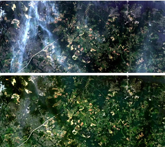
Figure 3. Image provided by the European Space Agency.Top: Represents the Sentinel-2 Level-1C uncorrected image. Bottom: Represents the Sentinel-2 Level-2A corrected image. This lower image requires an additional time-consuming computational step to correct for atmospheric distortions in the spectral data. Our method does not require the use of this pre-processing step.

The Sentinel-2 mission is part of the Copernicus program by the European Commission (EC). A global earth observation service addressing six thematic areas: land, marine, atmosphere, climate change, emergency management and security through its Sentinel missions. ESA is responsible for the observation infrastructure of the Sentinels (Copernicus, 2018). The data provided by the Sentinels has a free and open data policy implying that the data from the Sentinel missions is available free of charge to everyone. The ease of data access and use, allows all users from the public, private or research communities to reap the socio-economic benefits of such data (Wiatr et al., 2016). A Sentinel-2 image is provided to the end user at Level-1C (European Space Agency, 2018c) and has already gone through a series of pre-processing steps before it reaches the end user. However, these images have not been corrected for atmospheric distortions. This correction requires additional processing time to convert the image into Level-2A product, resulting in bottom of the atmosphere reflectances, see Figure 3 for a comparison. Within this work we directly use the Level-1C images for our computationally and cost efficient approach, mitigating the need to do the computationally costly processing.

Multi-spectral Data

The Sentinel-2 satellites map the entire global land mass every 5-days at various resolutions of 10 to 60$m$ per pixel, which means that each pixel represents an area of between $10m^{2}$ to $60m^{2}$. At each resolution, spectral information at the top of the atmosphere (TOA) is provided, creating a total of 13 spectral bands covering the visible, near infrared (NIR) and the shortwave infrared (SWIR) part of the electromagnetic spectrum (European Space Agency, 2018c; Zhang et al., 2017; Drusch et al., 2012). Although there are 13 spectral bands in total, we exclude bands 1, 9 and 10 as they interfere strongly with the atmosphere due to their 60$m$ resolution. This means that we only use the bands 2, 3, 4, 5, 6, 7, 8, 8A, 11, 12 as these bands have minimal interactions with the atmosphere and are provided at either a 10$m$ or 20$m$ spatial resolution.

2.1.2. Very-High-Resolution Satellite Images

In addition to freely available multi-spectral LR satellite images, we use VHR images with a resolution of up to 30cm per pixel, kindly provided by DigitalGlobe through Satellite Applications Catapult. See Figure 2 to see the difference in resolution between Sentinel-2 and VHR imagery.We emphasize that VHR imagery is only used in the cost-prohibitive method.

2.2. Annotated Satellite Imagery

We have annotated satellite imagery for the locations of informal settlements in parts of Kenya, South Africa, Nigeria, Sudan, Colombia and Mumbai. We then project these masks on to the satellite image and extract the necessary spectral information at those specific points, see Figure 4 for a example of an annotated ground truth map. We have open sourced the necessary code to do this here: https://frontierdevelopmentlab.github.io/informal-settlements/.

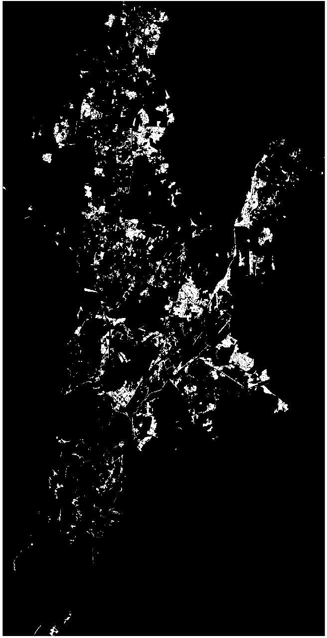
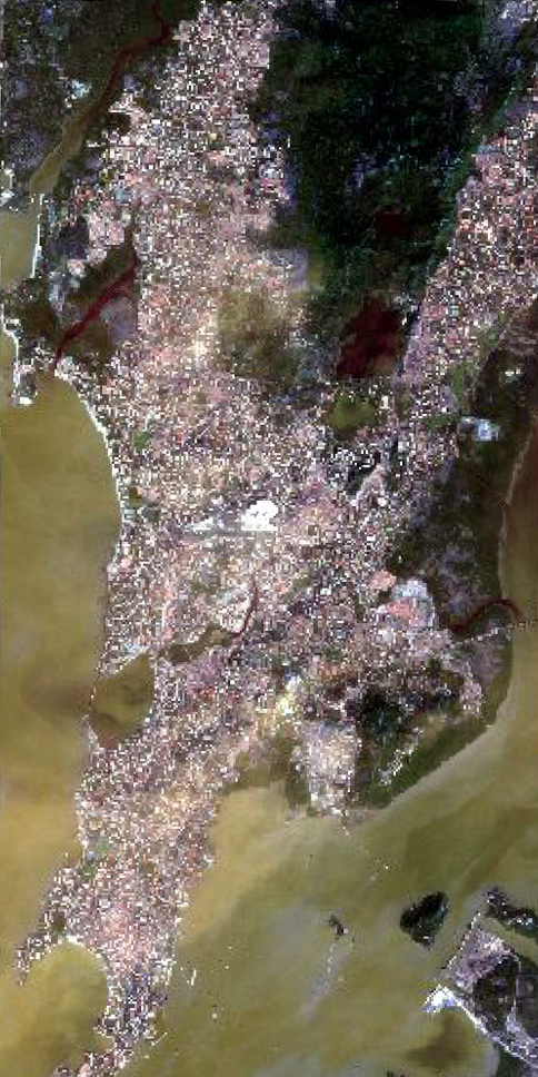
Figure 4. An example of annotated ground truth map. Left: The city is Mumbai, the white dots represent informal settlements and the black dots represent the environment. Right: The Sentinel-2 image of Mumbai.

3. Related Work

Recent publications applying machine learning to remote sensing data, in particular to satellite imagery, that have focused on detecting, or mapping informal settlements (Xie et al., 2015; Varshney et al., 2015; Mboga et al., 2017; Mahabir et al., 2018; Kuffer et al., 2016; Asmat and Zamzami, 2012; Kohli et al., 2016) have typically been trained on a specific region, or feature in combination with VHR (Stasolla and Gamba, 2008; Gevaert et al., 2016; Stasolla and Gamba, 2008; Kuffer et al., 2016). The approaches most in spirit to our own are (Varshney et al., 2015; Xie et al., 2015; Jean et al., 2016). Varshney et al. focus on detecting roofs in Eastern Africa using a template matching algorithm and random forest, they take advantage of Google Earths’ API to extract high resolution imagery, which although is free to researchers, is not openly available to everyone. Xie et al. and Jean et al. use a mixture of data sources and transfer learning across different data sets to generate poverty maps by taking advantage of night time imagery through the National Oceanic and Atmospheric Administration (NOAA) and daytime imagery through Google Earths’ API. However, to our knowledge there exists no previous work on predicting informal settlements solely from LR data, or predicting informal settlements in the way that we present here. This inhibits our ability to benchmark against previous methods. Thus, by providing the data sets and the baselines in this paper, we provide a robust way to compare the effectiveness of any future approaches and facilitate the creation of new machine learning methodologies.

4. Methods

In this section, we describe our approaches for detecting and mapping informal settlements. We introduce two different methods; a cost-efficient method and cost-prohibitive method. Our first method trains a classifier to learn what the spectrum of an informal settlement is, using LR freely available Sentinel-2 data. To do this, we employ a pixel-wise classification, where the system learns whether or not a 10-band spectra is associated to an informal settlement or the environment, which encompasses everything that is not an informal settlement. Our second method, is a semantic segmentation deep neural network that uses VHR satellite imagery, which is useful when informal settlements do not have unique spectra when compared to the environment, like those in Sudan, see Figure 5.

4.1. Cost Effective Method

Canonical Correlation Forests (CCFs) (Rainforth and Wood, 2015) are a decision tree ensemble method for classification and regression. CCFs are the state-of-the-art random forest technique, which have shown to achieve remarkable results for numerous regression and classification tasks (Rainforth and Wood, 2015). Individual canonical correlation trees are binary decision trees with hyper-plane splits based on local canonical correlation coefficients calculated during training. Like most random forest based approaches, CCFs have very few hyper-parameters to tune and typically provide very good performance out of the box. All that has to be set is the number of trees, $n_{trees}$. For CCFs, setting $n_{trees}=15$ provides a performance that is empirically equivalent to a random forest that has $n_{trees}=500$ (Rainforth and Wood, 2015), meaning CCFs have lower computational costs, whilst providing better classification. CCFs work by using canonical correlation analysis (CCA) and projection bootstrapping during the training of each tree, which projects the data into a space that maximally correlates the inputs with the outputs. This is particularly useful when we have small data-sets, like in our case, as it reduces the amount of artificial randomness required to be added during the tree training procedure and improves the ensemble predictive performance (Rainforth and Wood, 2015).

The computational efficiency aspects of CCFs and their suitability to both small and large data-sets, makes them ideal for detecting informal settlements for three reasons. First, many of the organisations that we aim to help will not have access to a large amount of compute resources, therefore computational efficiency is important. Second, to run the CCFs for both training and prediction, all that has to be called is one function. This ensures that the end user does not need to be an expert in ensemble methods and makes the method akin to plug and play. Finally, some of our ground truth data sets are relatively small, which means that we must use the data as efficiently as possible, which CCFs allow us to do. When VHR and computational cost are not a restriction we can employ a deep learning approach using convolution neural networks (CNN) to detect informal settlements.

4.2. Cost Prohibitive Method

Since informal settlements can also be classified by the rooftop size and the surrounding building density, we employ a state-of-the-art semantic segmentation neural network on optical (RGB) VHR satellite imagery to detect these contextual features. These contextual features are important when it is not possible to distinguish informal settlements from the environment by spectral signal in the same region. An example of such an informal settlement is shown in Figure 5. We see that the informal settlements in a rural region of Al Geneina, Sudan have a very low building density, and also the roof tops of both formal and informal settlements are built out of concrete, meaning they have the same spectral signal. This is in contrast to the dense slums in Nairobi and Mumbai.

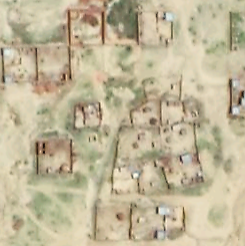
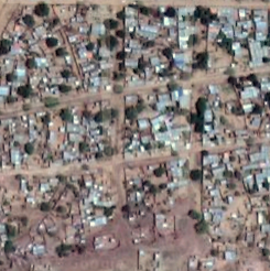
Figure 5. A VHR image comparing an informal, left and formal settlement, right, in Al Geneina, Sudan. The main distinguishing feature is the wider contextual information, as the material spectrum’s are the same.

4.2.1. Encoder-Decoder with Atrous Separable Convolution

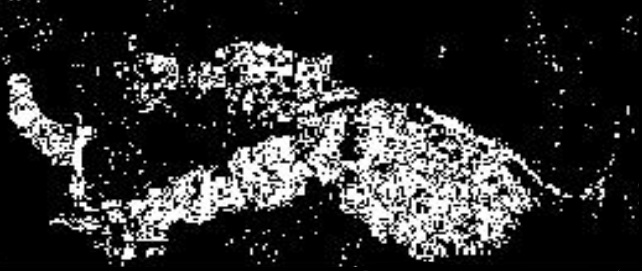
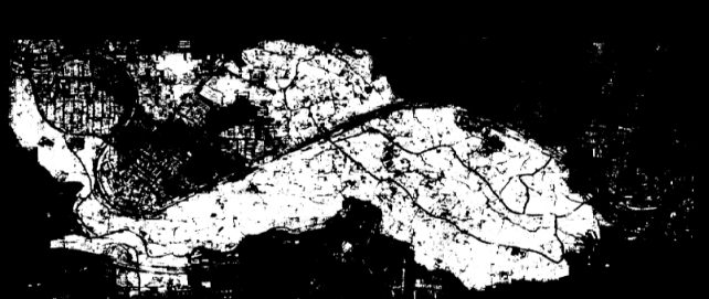
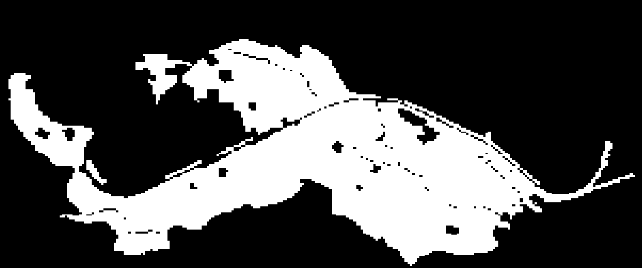
Figure 6. Predictions of informal settlements (white pixels) in Kibera, Nairobi. Left: The CCF prediction of informal settlements in Kibera on low-resolution Sentinel-2 spectral imagery. Middle: Deep learning based prediction of informal settlements in Kibera, trained on VHR imagery. Right: The ground truth informal settlement mask for Kibera.

For the task of semantic segmentation of informal settlements we use the DeepLabv3+ encoder-decoder architecture. DeepLabv3+  (Chen et al., 2018) is a deep CNN that extends the prior DeepLabv3 network (Chen et al., 2017) with a decoder module to refine the segmentation results of the previous encoder-decoder architecture particularly at the object boarders. The DeepLabv3 architecture uses Atrous Spatial Pyramid Pooling (ASPP) with Atrous convolutions to explicitly control the resolution at which feature responses are computed within the CNN. This ASPP module is augmented with image level features to capture longer range information. We use a Xception 65 network backbone in the encoder-decoder architecture. The beneficial use of this Xception model together with applying depth wise separable convolution to ASPP and the decoder modules have been shown in (Chen et al., 2018).

4.2.2. Implementation details

We train the entire network end-to-end with the usual back-propagation algorithm using eight Tesla V100 GPUs with 16 GBs of memory each. We initialize the layer weights using those from the pre-trained PASCAL VOC 2012 model (Everingham et al., 2012). We then fine-tune in turn the finer strides on the training/validation data. We train our deep network with a batch size of 32, an initial learning rate of 0.001 and a learning rate decay factor of 0.1 every 2.000 steps until convergence. Our experiments are based on a single-scale evaluation. All other hyper-parameters are the same as in the DeepLabv3+ model (Chen et al., 2018).

5. Results

Experimental Setup

For each region we have a 10-20$m$ resolution Sentinel-2 image, the corresponding VHR 30-50$cm$ resolution image and the ground truth annotations. We have ensured that the images and annotations are aligned in space and time to reduce any additional noise in the data. When training and validating a model on the same region we use a 80-20 split. We ensure that each class contains the same number of points, we then randomly sample 80% of each class to generate the training data and then use the remaining 20% of each class to construct our test set, which is comprised of a different set of points. We then center the training data (testing data accordingly) to have a mean of zero and standard deviation of one. We set the $n_{trees}=10$ for training the CCF. For validating our methods we report both pixel accuracy, and mean intersection over union (IoU). We use the standard definition of mean IOU, $meanIOU=\frac{1}{n_{class}}\frac{t_{ii}}{(t_{i}+\sum_{j}n_{ji}-n_{ii})}$ and pixel classification, $pxclass=\frac{\sum_{i}n_{ii}}{t_{i}}$, where $n_{class}$ is the total number of classes, $n_{ij}$ is the number of pixels of class $i$ predicted to belong to class $j$, and $t_{i}$ is the total number of pixels of class $i$ in ground truth segmentation.

We provide a comparison of both the pixel-wise classification with CCFs and the contextual classification with CNNs for the detection and mapping of informal settlements, see Table 1. The CCFs trained solely on freely available and easily accessible low-resolution data perform well, although they are unable to match the performance of the CNN trained on VHR imagery, except for Kibera. Figure 6 shows the predictions of both methods and the ground truth annotations. Despite having access to very high resolution data, the CNN still manages to miss-classify structural elements of the informal settlements in Kibera. Whereas the CCF, although more granular, incorporates the full structure of the informal settlement in Kibera via only the spectral information.

5.0.1. Generalizability

To demonstrate the adaptability of our approach we train each model on different parts of the world and use that model to perform predictions on other unseen regions across the globe. For this paper we train two models, one on Northern Nairobi, Kenya and another on Medellin, Colombia. The results can be found in Table 2. Even though we only have a small amount of data, we are able to demonstrate that our models can generalize moderately well, even with data that is noisy and partially incomplete. We provide several more results in the appendix A of this paper.

	Pixel Acc.		Mean IOU
Region	CCF	CNN	CCF	CNN
Kenya, Northern Nairobi	69.4	93.1	62.0	80.8
Kenya, Kibera	69.0	78.2	73.3	65.5
South Africa, Capetown*	92.0	-	33.2	-
Sudan, El Daien	78.0	86.0	61.3	73.4
Sudan, Al Geneina	83.2	89.2	35.7	76.3
Nigeria, Makoko*	76.2	87.4	59.9	74.0
Colombia, Medellin*	84.2	95.3	74.0	83.0
India, Mumbai*	97.0	-	40.3	-

Table 1. Pixel accuracy and mean IOU (%) results for informal settlement detection using the CCF pixel-wise classification and the contextual classification with CNNs. CCFs are trained and tested on low resolution imagery, CNNs are trained and tested on VHR imagery. *Represents that the ground truth annotations are less than 75% complete for the region.

	Pixel Acc.		Mean IOU
Region	NN	M	NN	M
Kenya, Northern Nairobi	69.4	55.0	62.0	54.4
Kenya, Kibera	67.3	63.8	54.1	56.0
South Africa, Capetown*	41.3	71.5	43.1	32.0
Sudan, El Daien	14.2	1.1	37.9	34.0
Sudan, Al Geneina	27.1	6.0	34.9	41.0
Nigeria, Makoko*	59.0	77.0	37.8	34.6
Colombia, Medellin*	65.0	84.2	46.9	74.0
India, Mumbai*	37.9	63.0	32.4	34.4

Table 2. Pixel accuracy and mean IOU (%) results for informal settlement detection using pixel-wise classification with CCFs trained on a particular region and testing on all other regions. Results are for a model trained on Northern Nairobi (NN) and a model trained on Medellin (M). * Represents that the ground truth annotations are less than 75% complete for the region.

6. Conclusions and Future Work

Conclusion

In this work we have composed a series of annotated ground truth data-sets and have provided for the first time benchmarks for detecting informal settlements. We have provided a comprehensive list of the challenges faced in mapping informal settlements and some of the constraints faced by NGOs. In addition to this, we have proposed two different methods for detecting informal settlements, one a cost-effective method, the other a cost-prohibitive method. The first method used computationally efficient CCFs to learn the spectral signal of informal settlements from LR satellite imagery. The second used a CNN combined with VHR satellite imagery to extract finer grained features. We extensively evaluated the proposed methods and demonstrated the generalization capabilities of our methods to detect informal settlements not just in a local region, but globally. In particular, we demonstrated for the first time that informal settlements can be detected effectively using only freely and openly accessible multi-spectral low-resolution satellite imagery.

Future work

Because of the uncertainties within the ground truth annotations and the differences in informal settlements across the world, we believe that this problem would be very useful for testing transfer learning and meta-learning approaches. In addition to this, Bayesian approaches would enable us to characterize these uncertainties via probabilistic models. This would provide an effective way to create adaptable models that learn what it means for an informal settlement to be informal, as the model absorbs new information.

It is also interesting to note that a 1 $km^{2}$ area containing informal settlements could house up to 129089 people (Desgroppes and Taupin, 2011) and so each pixel could represent up to 13 people . This therefore allows us to also add population estimates to our maps, which UNICEF state is also crucial. This would enable governments and NGOs to understand how much infrastructure is required and how much aid needs to be provided. Although we could have added population estimates in this current work, we have chosen to omit them as it would be irresponsible of us to provide estimates when not enough ground truth data exists, regarding average population numbers in informal settlements. We are actively working with UNICEF to gather more ground truth data for this and additional annotations for informal settlements, as UNICEF would actively like to deploy a system like the one that we have developed here to provide both mapping and population estimates of rural and urban informal settlements.

7. Acknowledgements

This project was executed during the Frontier Development Lab, Europe program, a partnership between the $\phi$-Lab at ESA, the Satellite Applications (SA) Catapult, Nvidia Corporation, Oxford University and Kellogg College. We gratefully acknowledge the support of Adrien Muller and Tom Jones of SA Catapult for their useful comments, providing VHR imagery and ground truth annotations for Nairobi. We thank UNICEF, in particular Do-Hyung Kim and Clara Palau Montava, for valuable discussions and AIData for access to geo-located Afrobarometer data. We thank Nvidia for computation resources. We thank Yarin Gal, Adam Golinski and Ben Fernando for their for their helpful comments. Bradley Gram-Hansen was also supported by the UK EPSRC CDT in Autonomous Intelligent Machines and Systems (EP/L015897/1). Patrick Helber was supported by the NVIDIA AI Lab program and the BMBF project DeFuseNN (Grant 01IW17002).

Appendix A Informal Settlement Classification Results

In this section we provide all results generated by the CCF on all informal settlement data-sets at our disposal and provides results in terms of two metrics; pixel-wise classification and mean intersection-over-union. We present two sets of results for Capetown.

• Capetown with Ground Truth (CapetownGT) - This represents around $20km^{2}$ region of Capetown (11% of the city). This data is annotated and it was used in the main paper.

• Capetown - This represents the whole of Capetown, however, we only have annotations for the region mentioned above (CapetownGT).

Country		Colombia	India	Kenya			Nigeria	South Africa		Sudan
City		Medellin	Mumbai	N. Nairobi	Kibera	Kianda	Mokako	Capetown	CapetownGT	AlGeneina	ElDaein
Model	Mumbai
Informal		78.35	97.18	71.44	74.84	89.23	94.81	80.88	89.10	21.00	10.96
Environment		36.32	95.92	43.37	51.65	31.33	28.53	56.45	43.11	68.19	83.71
Model	Capetown
Informal		96.86	98.00	99.21	96.52	100.00	99.73	98.77	99.61	99.99	99.90
Environment		9.80	46.97	9.07	10.12	4.03	7.27	96.33	15.22	0.23	0.10
Model	CapetownGT
Informal		83.77	73.94	93.59	82.16	96.13	95.32	84.78	92.34	99.48	90.82
Environment		51.69	85.41	40.25	45.33	22.23	24.60	82.68	93.33	2.53	5.99
Model	N. Nairobi
Informal		64.65	37.91	69.45	67.63	90.33	58.55	36.06	41.33	27.07	14.18
Environment		63.64	62.44	69.27	73.44	50.75	53.85	75.21	81.57	68.77	89.17
Model	Kibera
Informal		48.23	40.82	63.65	67.84	79.56	57.71	46.50	45.07	30.96	31.31
Environment		72.04	27.18	76.56	75.56	67.73	58.38	54.76	55.92	62.13	65.53
Model	Kianda
Informal		45.23	43.18	62.57	61.09	90.97	46.64	24.45	26.79	68.75	53.73
Environment		82.06	60.65	85.33	83.49	75.48	62.19	77.23	86.27	36.50	57.57
Model	AlGeneina
Informal		81.21	66.80	80.73	79.76	85.36	56.07	52.94	60.52	83.17	94.68
Environment		46.79	48.97	49.71	31.87	17.26	38.46	76.21	63.86	79.43	5.25
Model	ElDaein
Informal		24.07	9.50	46.58	54.11	71.82	8.37	29.90	25.65	68.52	78.16
Environment		76.61	40.11	67.18	71.47	71.20	85.19	48.91	61.22	30.61	71.65
Model	Mokako
Informal		17.33	69.43	10.67	14.15	13.54	76.27	35.60	34.76	5.53	10.57
Environment		85.22	39.06	89.91	94.07	94.37	80.84	60.91	61.89	92.97	88.51
Model	Medellin
Informal		84.06	62.95	54.10	63.84	88.12	77.00	63.38	71.46	5.66	1.09
Environment		79.88	63.02	85.79	78.85	47.00	37.45	62.01	57.68	96.28	95.78

Table 3. Pixel classification scores. The Model row represents the model that has been trained on the stated city and the
columns represent the city on which that trained model is making a prediction on.

Country		Colombia	India	Kenya			Nigeria	South Africa		Sudan
City		Medellin	Mumbai	N. Nairobi	Kibera	Kianda	Mokako	Capetown	CapetownGT	AlGeneina	ElDaein
Model	Mumbai
Informal IOU		31.23	68.58	41.42	45.04	30.14	27.74	56.32	42.83	55.82	59.81
Environment IOU		42.45	12.17	16.08	40.91	29.50	41.21	1.82	6.15	9.84	8.04
Mean IOU		36.84	40.37	28.75	42.97	29.82	34.47	29.07	24.49	32.83	33.92
Model	Capetown
Informal IOU		9.57	46.93	9.06	9.92	4.03	7.26	32.00	15.22	0.23	0.09
Environment IOU		44.07	7.53	15.20	37.97	26.14	37.11	1.44	4.74	21.95	30.96
Mean IOU		26.82	27.23	12.13	23.94	15.09	22.18	16.72	9.98	11.09	15.53
Model	CapetownGT
Informal IOU		46.06	84.43	39.83	40.97	21.94	23.98	82.54	57.74	2.53	5.76
Environment IOU		51.03	17.16	20.20	42.36	29.22	40.19	4.60	8.81	22.33	29.34
Mean IOU		48.55	50.80	30.02	41.67	25.58	32.08	43.57	33.28	12.38	17.55
Model	N. Nairobi
Informal IOU		50.26	60.77	80.99	61.79	49.14	43.86	74.67	78.82	57.08	64.38
Environment IOU		43.60	3.98	42.15	46.46	36.87	31.83	1.41	7.44	12.81	11.43
Mean IOU		46.93	32.38	61.57	54.12	43.00	37.84	38.04	43.13	34.95	37.90
Model	Kibera
Informal IOU		51.83	26.49	72.33	78.51	63.33	47.37	54.42	54.16	52.05	50.09
Environment IOU		35.17	2.33	26.25	68.11	40.79	32.84	1.03	4.15	13.18	17.71
Mean IOU		43.50	14.41	49.33	73.31	52.06	40.11	27.73	29.16	32.61	33.90
Model	Kianda
Informal IOU		58.10	59.17	80.38	68.05	68.33	48.09	76.57	82.69	33.56	47.67
Environment IOU		36.53	4.35	33.07	47.61	50.43	27.63	1.06	6.25	21.07	27.62
Mean IOU		47.31	31.76	56.72	57.83	59.38	37.86	38.81	44.47	27.31	37.65
Model	AlGeneina
Informal IOU		40.99	48.26	48.19	28.51	16.44	30.98	75.80	62.40	41.20	5.12
Environment IOU		47.58	5.31	19.90	36.78	24.84	26.45	2.12	6.15	30.17	30.43
Mean IOU		44.29	26.79	34.04	32.64	20.64	28.71	38.96	34.28	35.69	17.78
Model	ElDaein
Informal IOU		48.74	38.57	61.75	56.39	64.98	56.66	48.52	58.64	28.13	68.01
Environment IOU		18.36	0.65	15.55	36.33	38.86	6.59	0.58	2.56	19.73	54.78
Mean IOU		33.55	19.61	38.65	46.36	51.92	31.63	24.55	30.60	23.93	61.39
Model	Mokako
Informal IOU		52.52	38.54	78.39	62.69	72.95	63.65	60.46	59.59	73.49	63.16
Environment IOU		14.48	4.69	6.61	12.84	11.61	56.05	0.90	3.55	4.42	8.42
Mean IOU		33.50	21.61	42.50	37.77	42.28	59.85	30.68	31.57	38.96	35.79
Model	Medellin
Informal IOU		75.06	62.00	79.78	65.12	45.18	33.33	61.76	56.72	76.12	66.33
Environment IOU		72.73	6.71	29.03	46.84	34.41	36.01	1.64	6.46	4.99	0.99
Mean IOU		73.90	34.36	54.40	55.98	39.79	34.63	31.70	31.59	40.56	33.66

Table 4. Intersection Over Union (IOU) results. The Model row represents the model that has been trained on the stated city and the columns represent the city on which that trained model is making a prediction on.

Appendix B Very High-Resolution vs. Low-Resolution Images

Here we provide a comparison of differing image qualities, 50cm VHR image provided by DigitalGlobe and 10m LR image freely available via the Sentinel hub, for a subset of Kibera. In comparing the two images it is clear to see why we must use the additional spectral data contained within the LR images, if we are to extract any useful information regarding whether or not that pixel contains a settlement.

Figure 7. A very high-resolution (VHR) image of the Kibera slum. As depicted in Figures 2 and 5 in the main paper. A full resolution excerpt of this VHR satellite imagery is shown in Figure 8.

Figure 8. A low-resolution Sentinel-2 image of the Kibera slum as used in this study. As depicted in Figure 2 and 5 from the main paper.

References

- (1)
- Asmat and Zamzami (2012) A. Asmat and S.Z. Zamzami. 2012. Automated House Detection and Delineation using Optical Remote Sensing Technology for Informal Human Settlement. Procedia - Social and Behavioral Sciences 36 (2012), 650 – 658. https://doi.org/10.1016/j.sbspro.2012.03.071 ASEAN Conference on Environment-Behaviour Studies (AcE-Bs), Savoy Homann Bidakara Hotel, 15-17 June 2011, Bandung, Indonesia.
- Chen et al. (2017) Liang-Chieh Chen, George Papandreou, Florian Schroff, and Hartwig Adam. 2017. Rethinking atrous convolution for semantic image segmentation. arXiv preprint arXiv:1706.05587 (2017).
- Chen et al. (2018) Liang-Chieh Chen, Yukun Zhu, George Papandreou, Florian Schroff, and Hartwig Adam. 2018. Encoder-Decoder with Atrous Separable Convolution for Semantic Image Segmentation. In ECCV.
- Copernicus (2018) Copernicus. 2018. http://www.copernicus.eu/. Accessed : 2018-08-27.
- Desgroppes and Taupin (2011) Amélie Desgroppes and Sophie Taupin. 2011. Kibera: The biggest slum in Africa? Les Cahiers de l’Afrique de l’Est 44 (2011), 23–34.
- Drusch et al. (2012) M. Drusch, U. Del Bello, S. Carlier, O. Colin, V. Fernandez, F. Gascon, B. Hoersch, C. Isola, P. Laberinti, P. Martimort, A. Meygret, F. Spoto, O. Sy, F. Marchese, and P. Bargellini. 2012. Sentinel-2: ESA’s Optical High-Resolution Mission for GMES Operational Services. Remote Sensing of Environment 120 (2012), 25 – 36. https://doi.org/10.1016/j.rse.2011.11.026 The Sentinel Missions - New Opportunities for Science.
- European Space Agency (2018a) European Space Agency. 2018a. https://earth.esa.int/web/sentinel/user-guides/sentinel-2-msi/product-types/level-2a. Accessed : 2018-08-21.
- European Space Agency (2018b) European Space Agency. 2018b. https://sentinel.esa.int/web/sentinel/missions/sentinel-2. Accessed : 2018-08-27.
- European Space Agency (2018c) European Space Agency. 2018c. https://sentinel.esa.int/documents/247904/685211/Sentinel-2_User_Handbook. Accessed : 2018-08-27.
- Everingham et al. (2012) M. Everingham, L. Van Gool, C. K. I. Williams, J. Winn, and A. Zisserman. 2012. The PASCAL Visual Object Classes Challenge 2012 (VOC2012) Results.
- Fincher (2003) Ruth Fincher. 2003. Planning for cities of diversity, difference and encounter. Australian Planner 40, 1 (2003), 55–58. https://doi.org/10.1080/07293682.2003.9995252
- Gevaert et al. (2016) CM Gevaert, C Persello, R Sliuzas, and G Vosselman. 2016. Classification of informal settlements through the integration of 2D and 3D features extracted from UAV data. ISPRS Annals of the Photogrammetry, Remote Sensing and Spatial Information Sciences 3 (2016), 317.
- Hofmann et al. (2008) Peter Hofmann, Josef Strobl, Thomas Blaschke, and Hermann Kux. 2008. Detecting informal settlements from QuickBird data in Rio de Janeiro using an object based approach. In Object-based image analysis. Springer, 531–553.
- Huchzermeyer (2006) Marie Huchzermeyer. 2006. Informal settlements: A perpetual challenge? Juta and Company Ltd.
- Jean et al. (2016) Neal Jean, Marshall Burke, Michael Xie, W. Matthew Davis, David B. Lobell, and Stefano Ermon. 2016. Combining satellite imagery and machine learning to predict poverty. Science 353, 6301 (2016), 790–794. https://doi.org/10.1126/science.aaf7894 arXiv:http://science.sciencemag.org/content/353/6301/790.full.pdf
- Kohli et al. (2016) Divyani Kohli, Richard Sliuzas, and Alfred Stein. 2016. Urban slum detection using texture and spatial metrics derived from satellite imagery. Journal of Spatial Science 61, 2 (2016), 405–426. https://doi.org/10.1080/14498596.2016.1138247
- Kuffer et al. (2016) Monika Kuffer, Karin Pfeffer, and Richard Sliuzas. 2016. Slums from space—15 years of slum mapping using remote sensing. Remote Sensing 8, 6 (2016), 455.
- Mahabir et al. (2018) Ron Mahabir, Arie Croitoru, Andrew T Crooks, Peggy Agouris, and Anthony Stefanidis. 2018. A critical review of high and very high-resolution remote sensing approaches for detecting and mapping Slums: Trends, challenges and emerging opportunities. Urban Science 2, 1 (2018), 8.
- Mboga et al. (2017) Nicholus Mboga, Claudio Persello, John Ray Bergado, and Alfred Stein. 2017. Detection of informal settlements from VHR images using convolutional neural networks. Remote sensing 9, 11 (2017), 1106.
- Pais (2002) Marta Santos Pais. 2002. Poverty and Exclusion Among Urban Children. (2002).
- Rainforth and Wood (2015) Tom Rainforth and Frank Wood. 2015. Canonical correlation forests. arXiv preprint arXiv:1507.05444 (2015).
- Sclar et al. (2005) Elliott D. Sclar, Pietro Garau, and Gabriella Carolini. 2005. The 21st century health challenge of slums and cities. The Lancet 365, 9462 (05 Mar 2005), 901–903. https://doi.org/10.1016/S0140-6736(05)71049-7
- Stasolla and Gamba (2008) M. Stasolla and P. Gamba. 2008. Spatial Indexes for the Extraction of Formal and Informal Human Settlements From High-Resolution SAR Images. IEEE Journal of Selected Topics in Applied Earth Observations and Remote Sensing 1, 2 (June 2008), 98–106. https://doi.org/10.1109/JSTARS.2008.921099
- United Nations (2012) United Nations. 2012. State of the World’s Cities 2012-2013: Prosperity of Cities. United Nations Publications. https://books.google.co.uk/books?id=6cGzNAEACAAJ
- United Nations (2018) United Nations. 2018. United Nations Sustainable Development Goals. https://www.un.org/sustainabledevelopment/sustainable-development-goals/. Accessed : 2018-08-21.
- Varshney et al. (2015) Kush R Varshney, George H Chen, Brian Abelson, Kendall Nowocin, Vivek Sakhrani, Ling Xu, and Brian L Spatocco. 2015. Targeting villages for rural development using satellite image analysis. Big Data 3, 1 (2015), 41–53.
- Wekesa et al. (2011) B.W. Wekesa, G.S. Steyn, and F.A.O. (Fred) Otieno. 2011. A review of physical and socio-economic characteristics and intervention approaches of informal settlements. Habitat International 35, 2 (2011), 238 – 245. https://doi.org/10.1016/j.habitatint.2010.09.006
- Wiatr et al. (2016) T. Wiatr, G. Suresh, R. Gehrke, and M. Hovenbitzer. 2016. COPERNICUS PRACTICE OF DAILY LIFE IN A NATIONAL MAPPING AGENCY? ISPRS - International Archives of the Photogrammetry, Remote Sensing and Spatial Information Sciences XLI-B1 (2016), 1195–1199. https://doi.org/10.5194/isprs-archives-XLI-B1-1195-2016
- Xie et al. (2015) Michael Xie, Neal Jean, Marshall Burke, David Lobell, and Stefano Ermon. 2015. Transfer learning from deep features for remote sensing and poverty mapping. arXiv preprint arXiv:1510.00098 (2015).
- Zhang et al. (2017) Tianxiang Zhang, Jinya Su, Cunjia Liu, Wen-Hua Chen, Hui Liu, and Guohai Liu. 2017. Band selection in sentinel-2 satellite for agriculture applications. 2017 23rd International Conference on Automation and Computing (ICAC) (2017), 1–6.