Manifold spirals, disc-halo interactions and the secular evolution in N-body models of barred galaxies

Abstract

The manifold theory of barred-spiral structure provides a dynamical mechanism explaining how spiral arms beyond the ends of galactic bars can be supported by chaotic flows extending beyond the bar’s co-rotation zone. We discuss its applicability to N-body simulations of secularly evolving barred galaxies. In these simulations, we observe consecutive ‘incidents’ of spiral activity, leading to a time-varying disc morphology. Besides disc self-excitations, we provide evidence of a newly noted excitation mechanism related to the ‘off-centering’ effect: particles ejected in elongated orbits at major incidents cause the disc center-of-mass to recoil and be set in a wobble-type orbit with respect to the halo center of mass. The time-dependent $m=1$ perturbation on the disc by the above mechanism correlates with the excitation of new incidents of non-axisymmetric activity beyond the bar. At every new excitation, the manifolds act as dynamical avenues attracting particles which are directed far from corotation along chaotic orbits. The fact that the manifolds evolve morphologically in time, due to varying non-axisymmetric perturbations, allows to reconcile manifolds with the presence of multiple patterns and frequencies in the disc. We find a time-oscillating pattern speed profile $\Omega_{p}(R)$ at distances $R$ between the bar’s corotation, at resonance with the succession of minima and maxima of the non-axisymmetric activity beyond the bar. Finally, we discuss disc thermalization, i.e., the evolution of the disc velocity dispersion profile and its connection with disc responsiveness to manifold spirals.

1 Introduction

The manifold theory of spiral structure (Romero-Gomez et al. (2006); Voglis et al. (2006a); see also Danby (1965)) provides a dynamical mechanism to interpret how structures such as the bi-symmetrical spiral arms, observed beyond the ends of a galactic bar, can arise out of chaotic motions of the underlying distribution of matter. Two versions of the manifold theory have been developed so far in the literature.

i) In the ‘flux-tube’ version (Romero-Gomez et al. (2006); Romero-Gomez et al. (2007); Athanassoula et al. (2009a); Athanassoula et al. (2009b); Athanassoula et al. (2010); Athanassoula (2012)), one considers continuous-in-time orbits describing the flow of matter away from the bar’s unstable Lagrangian points L₁ and L₂, as viewed in a frame of reference rotating with angular speed equal to the bar’s pattern speed $\Omega_{p}$. The unstable ‘flux-tube’ manifolds are invariant sets formed by all orbits tending asymptotically towards $L_{1}$ or $L_{2}$ in the backward sense of time. This means that, in the forward sense of time, these orbits form an outflow directed away from $L_{1}$ or $L_{2}$. An elementary linearization of the equations of motion around $L_{1}$ or $L_{2}$ shows that these outflows, or ‘flux-tubes’, have the form of trailing spiral arms. Besides $L_{1}$ and $L_{2}$, similar flux-tube manifolds can be constructed for the whole family of epicyclic periodic orbits (called ‘Lyapunov orbits’) around $L_{1}$ or $L_{2}$.

ii) In the version of the manifold theory called ‘apocentric manifolds’ (Voglis et al. (2006a); Tsoutsis et al. (2008); Tsoutsis et al. (2009); Efthymiopoulos (2010); Harsoula et al. (2016)) one computes first the flux-tube manifolds, and then isolates only those points which correspond to apsidal positions, i.e., local apocentric or pericentric points of each orbit in the flux-tube. One can show that the pattern formed by the union of the apocentric points yields again trailing spiral arms. Near $L_{1}$ or $L_{2}$ the shapes of the flux-tube and apocentric manifolds coincide. However, far from the Lagrangian points, the shapes of the apocentric manifolds allow to visualize the intricate chaotic dynamics known in dynamical systems’ terminology as the ‘homoclinic tangle’ (see Wiggins (1990)). Thus, the flux-tube and the apocentric manifolds are the same phase-space objects, but visualized differently in physical space. For a detailed comparison and generalizations of the various manifold theories see Harsoula et al. (2016), or the tutorial Efthymiopoulos (2010).

Since the manifold spirals arise in a system of reference which co-rotates with the bar, the manifold theory in its basic form predicts that the spiral arms should have the same pattern speed as the bar. This remark seems to come in conflict with observations both in our Galaxy (as reviewed e.g. in Bland-Hawthorn & Gerhard (2016); see also Antoja et al. (2014), Junqueira et al. (2015) and references therein) and in other galaxies (e.g. Vera-Villamizar et al. (2001); Boonyasait et al. (2005); Patsis et al. (2009); Meidt et al. (2009); Speights and Westpfahl (2012); Speights & Rooke (2016)). Regarding, now, galactic disc simulations, the leading paradigm over the years refers to simulations showing the co-existence of multiple pattern speeds (Sellwood & Sparke (1988); Little & Carlberg (1991); Rautiainen & Salo (1999); Quillen (2003); Minchev & Quillen (2006); Dubinski et al. (2009); Quillen et al. (2011); Minchev et al. (2012); Baba et al. (2013); Roca-Fabrega et al. (2013); Font et al. (2014); Baba (2015); but see also a noticeable exception in Roca-Fabrega et al. (2013)), possibly connected also to the phenomenon of nonlinear coupling of multiple disc modes (Tagger et al. (1987); Tagger & Athanassoula (1991); Sellwood & Wilkinson (1993); Masset & Tagger (1997)). On the other hand, it is well known that even isolated barred galaxies undergo substantial secular evolution (see Athanassoula (2013); Binney (2013); Kormendy (2013) in the tutorial volume Falcon-Barroso and Knapen (2013)). The tendency to transfer angular momentum outwards (e.g. towards the halo or across the disc, Tremaine & Weinberg (1984); Debattista & Sellwood (1998); Debattista & Sellwood (2000); Athanassoula (2002); Athanassoula & Misiriotis (2002); Athanassoula (2003); OŃeill & Dubinski (2003); Holley-Bockelmann et al. (2005); Berentzen et al. (2006); Martinez-Valpuesta et al. (2006)) leads the bar to slow down and grow in size at a rate which produces non-negligible change in dynamics at timescales comparable even to a few bar periods. This process becomes complex, and even partially reversed due to the growth of ‘pseudo-bulges’ or peanuts (Kormendy & Kennicutt (2004)), caused by dynamical instabilities such as chaos or the ‘buckling instability’ Combes & Sanders (1981); Combes et al. (1990); Pfenniger & Friedli (1991); Raha et al. (1991); Bureau & Athanassoula (1999); Martinez-Valpuesta & Shlosman (2004); Bureau & Athanassoula (2005); Debattista et al. (2006)). The reduction in size of the bar by the transfer of angular momentum under constant pattern speed is discussed in Weinberg & Katz (2007). Spiral activity acts as an additional factor of outwards transfer of angular momentum (Lynden-Bell & Kalnajs (1972)), while a radial re-distribution of matter can take place even under a nearly-preserved distribution of angular momentum (Hohl (1971); Sellwood & Binney (2002); Avila-Reese et al. (2005)). Radial migration is enhanced by the amplification of chaos due to the overlapping of resonances among the various patterns (Quillen (2003); Minchev & Quillen (2006); Quillen et al. (2011)).

As secular evolution affects both the bar’s morphology and pattern speed, as well as the extent to which other non-axisymmetric patterns are present in the disc, the shapes of the invariant manifolds found by momentarily ‘freezing’ the potential and pattern speed value also undergo important changes in time. Simulations by Lia Athanassoula have shown that, despite these changes, the stars out-flowing from the neighborhood of the Lagrangian points $L_{1}$ and $L_{2}$ develop orbits which, in general keep track of the change of the form of the invariant manifolds (Athanassoula (2012); see also Baba (2015); Lokas (2016)). As a rule, the material which populates the manifolds comes from orbital outflows originating from the interior of co-rotation, at the end of the bar (Contopoulos (1980)). As these outflows are adapted to the slowly-changing form of the manifolds, they are able to yield time-varying spiral or ring-like patterns. In principle, this non-rigidity of the shape and population density of the invariant manifolds leaves space to reconcile manifold spirals with time and space varying pattern speeds beyond the bar, although such a reconciliation awaits probe by specific simulations.

In the present paper we aim to investigate the application of the manifold theory of spirals in a typical model of secularly evolving bar. To this end, a series of isolated disc galaxy simulations were performed using the explicit Mesh-Adaptive N-Body method based on Approximate Inverses (MAIN, Kyziropoulos et al. (2016)), and the Parallel Self-Mesh Adaptive N-body technique based on Approximate Inverses (PMAIN, Kyziropoulos et al. (2017a); Kyziropoulos et al. (2017b)). The initial conditions for these simulations are described in Kyziropoulos et al. (2016). Whenever a bar is formed in a simulation, we find manifold spirals, as well as traces of secular evolution affecting the bar and other non-axisymmetric features in the disc. In the present paper we focus on one of these simulations (‘Q1’ in Kyziropoulos et al. (2016)), aiming to present these phenomena in considerable detail. This is a typical simulation starting with a Toomre $Q=1$ exponential disc, a Dehnen-like ‘double-power-law’ halo, and a Sersic bulge, with parameters corresponding to a Milky-Way type galaxy (see Binney & Tremaine (2008)). The simulation undergoes phases of evolution known in literature since decades (see references above), namely: i) an initial instability leading to the formation of $m=2$ spirals, lasting for $\sim 1Gyr$, ii) a bar instability, erasing all traces of the previous spirals and generating new ones related to the bar, iii) a ‘bucking instability’ which thickens the bar, and iv) a phase of slow evolution in which the amplitude of spirals is reduced. We focus our study on the epoch after the bar is formed (around $t=1.5$Gyr), and up to $t=4Gyr$. We measure several quantities which quantify the bar’s secular evolution. We then observe the corresponding evolution of the manifolds emanating from the neighborhood of $L_{1}$ and $L_{2}$, as well as what happens, in general, to the disc as the bar-spiral structure evolves.

Our results lead to the following picture: as typical in such simulations, we find that spiral activity beyond the bar is characterized by recurrent episodes. ‘Incidents’ of growth of spiral and other non-axisymmetric disc features with substantial spectral power take place in a nearly damped-oscillatory manner. Damping, which results in these non-axisymmetric features gradually fading in amplitude, can be attributed to ‘disc heating’, i.e. the overall increase in time of the velocity dispersion in the outer parts of the disc (see Sellwood (2014) for a review). However, regarding what causes, in the first place, the repeated excitations of incidents of non-axisymmetric activity, besides recognizing in our simulation some well known mechanisms of enhancement of local perturbations (e.g. swing amplification, see also Baba (2015)), we find evidence of a mechanism not emphasized, to our knowledge, in literature. This is the fact that, every incident is accompanied by the creation of a population of particles moving in orbits either escaping or with apocenters far from the main part of the disc, whose distribution of directions of motion exhibits fluctuations with respect to perfect central symmetry. Hence, they cause the main part of the disc to recoil with respect to the spheroid (i.e. halo-bulge) center of mass. The recoil causes, in turn, an ‘off-centering effect’ resulting in a $m=1$ disturbance on the disc. Some studies have indicated the importance of such phenomena in the evolution of bar-halo systems, as well as the evolution of halo cusps (Sellwood (2003); McMillan & Dehnen (2005); Holley-Bockelmann et al. (2005); Debattista (2006); see also Hamilton et al. (2018) for a different application in the relaxation of globular clusters). Here we find that the ‘incidents’ of non-axisymmetric activity are correlated with the off-centering effect. The disc recoil sets the disc center of mass in relative orbit with respect to the spheroid (halo-bulge) center of mass. The relative orbit has small size (the ‘wobbling’ between disc and halo can extend as much as $\sim 0.3$ kpc, about $5-10\%$ of the bar size; off-centering effects of larger size are reported in McMillan & Dehnen (2005), with no apparent connection with the mechanism mentioned above). Yet, this is sufficient to induce a significant $m=1$ perturbation on the disc, with amplitude $\sim 0.1$ in a region including the bar. The disc response is found to have both $m=1$ and $m=2$ components. The latter might be connected to particles pushed to regions outside co-rotation, in which case they have to follow chaotic orbits guided by the (predominantly $m=2$) manifolds. Since at least one major recoil event is observed before the bar, the manifolds cannot be the drivers of the phenomenon. They can, however, help to maintain it, by supporting particles in chaotic orbits leading to fluctuations in the directions in which the particles move.

All together, we identify the role of the invariant manifolds as a skeleton of chaotic orbits in phase space, or, the dynamical avenues to be followed by particles whenever an incident of spiral or other non-axisymmetric is triggered in the disc. The morphology of observed patterns in the disc is always qualitatively similar to the ‘chaotic tangle’ formed by the manifolds, while direct comparison of the two patterns yields various levels of agreement, depending on the snapshot examined.

We finally study how all these phenomena evolve with the change in disc ‘temperature’ (velocity dispersion). The incidents of non-axisymmetric activity beyond the bar fade in a timescale $~{}4$ Gyr. However, this happens in a purely stellar dynamical simulation. Invoking mechanisms able to dissipate kinetic energy in random motions (e.g. gas cooling, star formation etc.) should help to prolong these phenomena over a considerable fraction of the age of real disc galaxies.

The paper is structured as follows: section 2 presents the N-body simulation as well as methods of analysis. Section 3 explains the computation of the invariant manifolds and its comparison with the disc morphology. Section 4 deals with the disc’s secular evolution, and shows the comparison with the manifolds at various times. Section 5 summarizes our conclusions, along with some further comments on the role of manifolds in the modelling of barred-spiral galaxies.

2 Simulation and numerical computations

2.1 Initial conditions and N-body simulation

The simulation analyzed below corresponds to the experiment called ‘Q1’ in Kyziropoulos et al. (2016). In summary, we use $10^{7}$ particles to simulate:

i) an initially exponential disc of mass $M_{disc}=5\times 10^{10}M_{\odot}$, exponential scale length $R_{d}=3$ kpc, vertical exponential scalelength $z_{d}=0.2$ kpc and Gaussian velocity distribution arising from a profile of Toomre’s Q-parameter rising in the center and tending to an asymptotic outward value $Q\rightarrow Q_{\infty}$ with $Q_{\infty}=1$ (see equation (13) of Kyziropoulos et al. (2016)).

ii) a Sersic-type spherical bulge embedded in the disc, mass $M_{b}=5\times 10^{9}$, Sersic index $n=3.5$, scale length $R_{b}=1$ kpc.

iii) A Dehnen-type double-power law spherical dark matter halo (see Binney & Tremaine (2008)), with density parameter $\rho_{0}=2.016\times 10^{8}$ $M_{\odot}/kpc^{3}$, scale length $R_{h}=3$ kpc, and asymptotic inner and outer density power-law exponents $\alpha=1.3$, $\beta=3.5$. The halo yields a mass $\approx 7\times 10^{10}M_{\odot}$ at $R=50$ kpc, which rises to $2\times 10^{11}M_{\odot}$ at $R=100$ kpc.

The disc, bulge and halo are represented by $5\times 10^{6}$, $5\times 10^{5}$ and $4.5\times 10^{6}$ particles respectively. A ‘relaxation technique’ is used to match all three components in a unique system with virial ratio very close to $2$ (see Kyziropoulos et al. (2016) and Kyziropoulos et al. (2017a) for a description). Being prone to disc instabilities, the system exhibits vivid evolution dominated by the succession of spiral, bar, and other non-axisymmetric features.

The simulation was performed using the N-body code MAIN, which utilizes a Cartesian grid that solves Poisson equation by the use of a novel Symmetric Factored Approximate Sparse Inverse (SFASI)pre-conditioning technique, in conjunction with the multigrid method. Details on the features of the numerical technique are provided in Kyziropoulos et al. (2016). In Kyziropoulos et al. (2017a) and Kyziropoulos et al. (2017b) we presented two fully parallel versions of the N-body technique (for shared-memory and distributed-memory systems respectively). These versions implement fully adaptive mesh refinement while improving the algorithm by which boundary conditions are computed on the sides of the computational box. Using these improved techniques, we performed $N=10^{8}$ and $N=10^{9}$ particle versions of the numerical simulation Q1 (see Kyziropoulos et al. (2017a) and Kyziropoulos et al. (2017b)). The new simulations differ from the original one essentially only with respect to the exact moment when the bar instability is manifested. This is partly due to the better resolution of the profile of the central force, which affects the onset of the bar instability (Holley-Bockelmann et al. (2005)), and also to the fact that a smoother particle distribution implies lesser noise, and hence longer time for any instabilities to grow in the disc (e.g. by swing amplification, Toomre and Kalnajs (1991)). On the other hand, the main features of the bar and spirals (Fourier amplitudes, pattern speeds, secular evolution etc) appear similar in all runs.

Several computations require use of a smooth approximation of the potential $\Phi(x,y,t)$ in the disc plane $(x,y)$. This is obtained, using bi-cubic interpolation, from the N-body potential evaluated in a grid $x_{i}=-L_{0}/2+(i/N_{p})L_{0}$, $y_{j}=L_{0}/2+(j/N_{p})L_{0}$, where $i,j=0,1,\ldots,N_{p}-1$, $L_{0}=25.6$ kpc, $N_{p}=256$.

2.2 Evolution of non-axisymmetric patterns

As a consequence of the chosen initial value of $Q$ (=1), the disc exhibits a rapid growth of competing features. A $m=2$ spiral mode dominates up to about $t=1.1$ Gyr. After some transient phase, the bar starts growing rapidly between $t=1.3$ Gyr and $t=1.6$ Gyr. This growth is followed by ‘incidents’ of spiral activity (see below). Five such ‘incidents’ take place up to $t=2$ Gyr. The overall morphology of the galaxy changes rapidly in timescales as small as the bar period. The morphological evolution of the disc is shown in Fig. 1. As typical in such simulations, features like rings and spiral arms appear reccurently and with varying morphology after the bar formation. We focus on the incidents of spiral activity which take place between $t=1.65$ and $t=3$ Gyr. The bar performs slightly more than seven (counterclockwise) revolutions in this time interval. The spiral modes oscillate from conspicuous maxima (e.g. at $t=1.65$, $t=1.95$, $t=2.25$ Gyr) to very low minima (e.g. at $t=2.025$, $2.325$, $2.7$, $2.925$ Gyr), albeit never vanishing completely. An inner ring-like structure surrounding the bar is also present, while, at particular snapshots (e.g. $t=1.825$) material appears to travel from one end of the bar to the other along the ring. This phenomenon is discussed in depth in several papers on the ‘flux-tube’ manifolds, e.g. Romero-Gomez et al. (2006); Athanassoula (2012).

The bar also thickens in time, forming a peanut, or ‘X-shaped’, pseudobulge). From an inspection of the vertical disc profiles and the evolution of the $m=2$ amplitude (see below), we infer that a buckling instability occurs around $t\approx 2$ to $2.1$ Gyr. Manifold spirals, however, keep appearing well after $t=2.1$ Gyr. Thus, the manifold spirals do not appear to be halted by the buckling instability, as was reported for other simulations in Kwak et al. (2017) (see also Lokas (2016)).

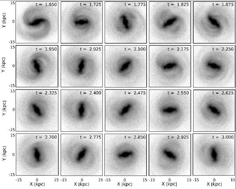
Figure 1: Twenty snapshots of the face-on disc view in the interval $1.65\leq t[Gyr]\leq 3.0$. The bar rotates counter-clockwise. Spiral and ring-like structures appear reccurently and with varying amplitudes.

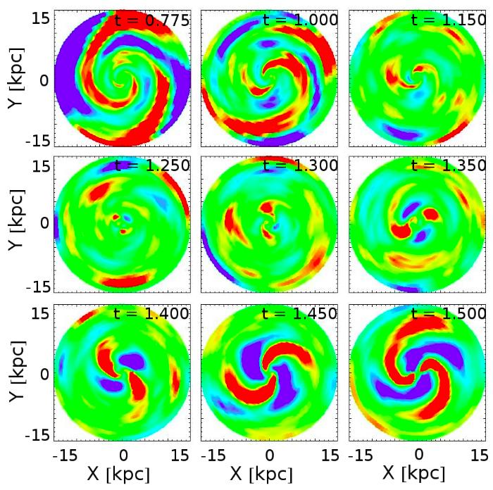
Figure 2: The non-axisymmetric excess density $D(R,\phi)$ in nine snapshots in the interval $0.775\leq t[Gyr]\leq 1.5$. The color scale represents values $D(R,\phi)\leq-0.5$ in blue, $D(R,\phi)\geq 0.5$ in red and $-0.5<D(R,\phi)<0.5$ in between. The transition from a spiral to a bar mode dominance is shown. The first manifold spirals are developed immediately after the bar formation.

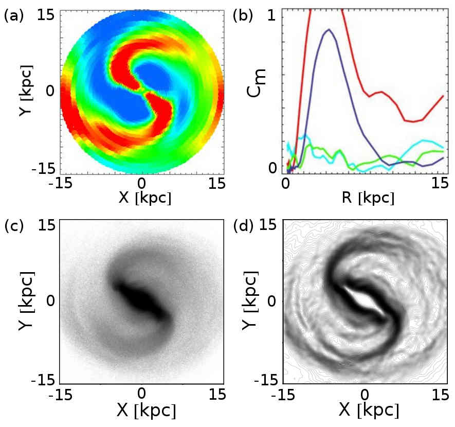
Figure 3: (a) Color map of the non-axisymmetric excess density at $t=1.625$ Gyr. A second incident of spiral activity accompanies the bar. (b) The Fourier amplitudes $C_{1}(R)$ (cyan), $C_{2}(R)$ (red), $C_{3}(R)$ (green) and $C_{4}(R)$ (blue). (c) The disc image by a logarithmic grayscale plot of the surface density $\Sigma(R,\phi)$. (d) The same image as in (c) after implementing the Sobel-Feldman edge detection algorithm (see text). Dimmer patterns of (c) are enhanced and clearly visible in (d).

We quantify the evolution of non-axisymmetric features using the disc surface density

$$\Sigma_{d}(R,\phi,t)={\Delta N(R,\phi,t)\over R\Delta R\Delta\phi}$$ (1)

where $\Delta N(R,\phi,t)$ is the number of disc particles at time $t$ in each area element $R\Delta R\Delta\phi$ of a polar grid of 50 logarithmically equi-spaced radial bins from $R_{1}=0.1$ kpc to $R=15$ kpc, and 180 azimuthal bins from $\phi=0$ to $\phi=2\pi$. Next, we compute the Fourier transform

$$\Sigma_{d}(R,\phi)=\Sigma_{d,0}(R)+\sum_{m=1}^{\infty}[A_{m}(R)\cos(m\phi)+B_{m}(R)\sin(m\phi)]~{}.$$ (2)

The relative amplitude $C_{m}(R)$ and phase $\phi_{m}(R)$ of the m-th Fourier mode are defined by

$$C_{m}={\left(A_{m}^{2}+B_{m}^{2}\right)^{1/2}\over\Sigma_{d,0}},~{}\phi_{m}={1\over m}\tan^{-1}\left({B_{m}\over A_{m}}\right)~{}.$$ (3)

Truncating Eq. (2) in a finite number of harmonics ($m\leq 10$) yields a smoothed representation of the surface density $\Sigma_{s}(R,\phi)$. The smoothed ‘non-axisymmetric excess density’ is defined as

$$D(R,\phi)={\Sigma_{s}(R,\phi)-\Sigma_{d,0}(R)\over\Sigma_{d,0}}~{}~{}~{}.$$ (4)

The rapid growth of non-axisymmetric features in the disc leads to a dominant $m=2$ spiral mode lasting up to the time $t=1.1$ Gyr (Fig. 2). However, the onset of the bar instability erases all traces of previous spiral activity. The bar grows rapidly between $t=1.3$ Gyr and $t=1.6$ Gyr. A first conspicuous set of spiral arms beyond the bar appears around $t=1.5$ Gyr. The bar extends to $R\approx 5$ kpc (as measured by the interval in $R$ in which the $m=2$ phase remains nearly constant), while co-rotation is initially at $R\approx$ 6.5kpc. At $t=1.625$ Gyr, a second major incident of spiral activity takes place. Beyond this time, the $m=2$ and $m=4$ Fourier amplitudes enter a phase of considerably slower evolution.

Setting conventionally $t=1.625$ as the time at which the bar’s secular evolution begins, in the next section we focus on this time snapshot to describe the computations related to manifold spirals and the comparison between manifolds and observed N-body disc morphologies. As shown in Fig.3, the bar is very strong at this snapshot, with $C_{2}>1$ and $C_{4}\approx 0.8$ at $R\approx 4$ kpc. There is also important power in the $m=1$ and $m=3$ Fourier terms. The $C_{1}$ amplitude is larger than 0.1 across the bar’s whole extent and reaches $\sim 0.2$ in the central parts ($R<2$ kpc). Such $m=1$ amplitudes are identifiable in several simulations (see, for example, Quillen et al. (2011); Minchev et al. (2012)). The question of what triggers the $m=1$ mode in the inner parts of the disc will be dealt with in section 4. On the other hand, in the snapshot of Fig. 3, substantial $m=1$ relative amplitudes are observed also at large distances ($R>10$ kpc). This is connected to the lopesidedness of the observed spirals (and manifolds, see below), a fact which hints towards nonlinear interaction of the outer disc modes.

In Fig. 3, the density excess map (a) clearly shows the main spiral pattern, but not so clearly secondary features as the interarm features or the bifurcation of spirals seen in the lower left part of the direct image of the disc (panel (c)). In order to bring out these features, we produce an image of the disc (panel (d)) which enhances the edges of most ‘eye-recognizable’ patterns of image (c) using a pattern-recognition algorithm known as the ‘Sobel-Feldman edge detection’(see Gonzalez & Woods (1992)). This technique is similar to unsharp masking in that it processes the image through a smoothing filter (we used a Gausssian filter for image (c)). Instead of substracting the two images, Sobel-Feldman uses an operator to approximate the gradient of the smoothed image, and thus detect the edges of patterns, where the gradient becomes large. The Sobel-Feldman technique enhances the ability to recognize non-axisymmetric features of amplitude significantly lower than the one of the main bi-symmetric spirals. In subsequent sections we will use such ‘Sobel-Ferldman’ images of the disc in comparison with the patterns formed by the manifolds in the corresponding snapshots.

3 Manifold spirals

3.1 Definitions

At a fixed time $t$, consider observers moving in a galactocentric frame rotating with angular velocity $\Omega_{p}$ equal to the instantaneous angular velocity of the bar. Let $V(x,y,z)$ be the total gravitational potential (arising from all components, e.g. bulge, disc-bar, halo) at the time $t$. We consider first orbits in the rotating frame with ‘frozen’ in time potential $V$. Let $\Phi(x,y)=V(x,y,z=0)$ be the potential restricted in the disc plane. The orbits are given by Hamilton’s equations with Hamiltonian

$$H={p_{R}^{2}\over 2}+{p_{\phi}^{2}\over 2R^{2}}-\Omega_{p}p_{\phi}+\Phi(R,\phi)~{}~{},$$ (5)

where $(R,\phi)$ are cylindrical co-ordinates in the rotating frame, $x=R\cos\phi$, $y=R\sin\phi$, and $(p_{R},p_{\phi})$ are the radial and angular momentum (per unit mass) in the intertial frame, connected to the velocities $V_{x},V_{y}$ in the rotating frame via $p_{R}=(xV_{x}+yV_{y})/R$, $p_{\phi}=\Omega_{p}R^{2}+(xV_{y}-yV_{x})$. The potential $\Phi(R,\phi)$ admits the Fourier decomposition:

$$\Phi(R,\phi)=\Phi_{0}(R)+\sum_{m=1}^{\infty}[\Phi_{m}(R)\cos(m\phi)+\Psi_{m}(R)\sin(\phi)]~{}.$$ (6)

Consider first a simplified bar-like model in which $\Phi_{m}(R)=\Psi_{m}(R)=0$ for all $m>0$ except $m=2$ and $\Phi_{2}(R)/\Psi_{2}(R)=const$. The bar has a fixed orientation angle $\phi_{bar}$ in the rotating frame. The equations of motion yield four Lagrangian equilibrium points (Binney & Tremaine (2008)). The unstable Lagrangian points are at the end of the bar, $R_{L1}=R_{L2}=R_{C}$, $p_{\phi,L1}=p_{\phi,L2}=\Omega_{p}R_{C}^{2}$. The stable Lagrangian points are at distance $R_{C}^{\prime}$. The annulus $R_{C}^{\prime}<R<R_{C}$ is hereafter called the corotation zone. Introducing the full non-axisymmetric perturbation may induce an important deformation of the equipotential surfaces, influencing the number and position of unstable Lagrangian points (Tsoutsis et al. (2009), Athanassoula et al. (2009a), Athanassoula et al. (2009b), Kalapotharakos et al. (2010), Wu et al. (2016)). In the present simulation we observe only a small displacement of the points $L_{1}$, $L_{2}$ with respect to the pure bar model.

The key property leading to the definition of the manifold spirals is now the following: one can show that there is a family of initial conditions for which the resulting orbits under the potential (6) tend asymptotically to the Lagrangian point $L_{1}$ when integrated backward in time, i.e., as $t\rightarrow-\infty$. This leads to the formal definition of the unstable manifold of $L_{1}$. Denote by $O(t;R_{0},\phi_{0},p_{R,0},p_{\phi,0})$ one orbit with initial conditions $(R_{0},\phi_{0},p_{R,0},p_{\phi,0})$, and also $O_{L1}\equiv(R_{L1},\phi_{L1},p_{R,L1},p_{\phi,L1})$. The unstable manifold ${\cal W}^{U}_{L1}$ is the ensemble of all different initial conditions for which the distance between $O(t;R_{0},\phi_{0},p_{R,0},p_{\phi,0})$ and $O_{L1}$ tends to zero as $t\rightarrow-\infty$:

$${\cal W}^{U}_{L1}=\Bigg{\{}\mbox{All~{}}(R_{0},\phi_{0},p_{R,0},p_{\phi,0}):~{}~{}~{}~{}~{}~{}~{}~{}~{}~{}~{}~{}~{}~{}~{}~{}~{}~{}~{}~{}~{}~{}~{}$$

$$dist[O(t;R_{0},\phi_{0},p_{R,0},p_{\phi,0}),O_{L1}]\rightarrow 0\mbox{~{}as~{}}t\rightarrow-\infty\Bigg{\}}~{}.$$ (7)

Similar definitions hold for the unstable manifold of the Lagrangian point $L_{2}$. Basic theorems of dynamics (Grobman (1959); Hartman (1960)) ensure that the sets ${\cal W}^{U}_{L1}$, ${\cal W}^{U}_{L2}$ are non-empty. The dynamical role of the invariant manifolds ${\cal W}^{U}_{L1}$ and ${\cal W}^{U}_{L2}$ can be summarized as follows: ${\cal W}^{U}_{L1}$ collects the ensemble of trajectories tending arbitrarily close to $L_{1}$ in the backward sense of time. Thus, starting very close to $L_{1}$, and integrating forward in time, these trajectories form an outflow away from $L_{1}$. Projected in real space, this outflow yields the ‘flux-tube’ manifold ${\cal W}^{UFT}_{L1}$ (Romero-Gomez et al. (2006); Romero-Gomez et al. (2007)). An elementary analysis shows that the flux-tube manifold has two branches: one is directed outwards (outside co-rotation), and it takes the shape of a trailing spiral arm. The second is directed inwards (inside corotation), creating a ring-like structure around the bar. Thus, the flux-tube manifolds can give rise to several morphological structures, from rings to open spirals, depending on the model’s parameters (e.g. pattern spead, $m=2$ amplitude and asymmetry) as discussed in (Athanassoula et al. (2009a)).

In a similar way as for ${\cal W}^{U}_{L1}$, we can define outflows of asymptotic trajectories emanating from a small but finite distance from $L_{1}$. To this end, we invoke the family of short period (or ‘Lyapunov’) unstable periodic orbits which form small retrograde epicycles around $L_{1}$, called hereafter the ‘PL1 orbits’ (Voglis et al. (2006a)) (denoted $O_{PL1}$). Similarly to $L_{1}$, the unstable manifold of such an orbit, is defined as

$${\cal W}^{U}_{PL1}=\Bigg{\{}\mbox{All~{}}(R_{0},\phi_{0},p_{R,0},p_{\phi,0}):~{}~{}~{}~{}~{}~{}~{}~{}~{}~{}~{}~{}~{}~{}~{}~{}~{}~{}~{}~{}~{}~{}~{}~{}$$

$$dist[O(t;R_{0},\phi_{0},p_{R,0},p_{\phi,0}),O_{PL1}]\rightarrow 0\mbox{~{}as~{}}t\rightarrow-\infty\Bigg{\}}~{}.$$ (8)

The projection of the manifolds ${\cal W}^{U}_{PL1,2}$ in the disc plane yields the ‘flux-tube’ manifolds ${\cal W}^{UFT}_{PL1,2}$. The geometric shapes and properties of the manifolds ${\cal W}^{UFT}_{PL1,2}$ are similar to those of the manifolds ${\cal W}^{UFT}_{L1,2}$. However, the periodic orbits PL1,2 and their manifolds form families which span a whole set of values of the Jacobi constant $E_{J}$, while the unstable points $L_{1,2}$ and their manifolds represent only the values of the Jacobi constants $E_{J,L1,2}$. One has $E_{J,PL1,2}>E_{J,L1,2}$ for any orbit of the PL1,2 families and their manifolds, implying that the manifolds ${\cal W}^{UFT}_{PL1,2}$ characterize the motions of particles at all energies beyond the Jacobi energy at corotation.

The ‘flux-tube’ manifolds defined above represent a continuous swarm of trajectories with initial conditions in the set (3.1), or (3.1). This set reproduces the manifolds as geometric objects, but provides no information on the real distribution of matter along the manifolds, which depends on the distribution function of the N-body system. Despite the fact that a precise knowledge of the distribution function is hardly tractable, the method of apocentric manifolds (Voglis et al. (2006a)) exploits the fact that local density maxima along the manifolds are expected at points close to apsidal (i.e. pericentric or apocentric) positions of the orbits. This assumption is verified in N-body experiments (see Tsoutsis et al. (2008)), where it is shown that density maxima corresponding, in particular, to spiral patterns are associated with local apocenters of the orbits of the N-body particles. The apocentric manifolds ${\cal W}^{UA}_{L1,2}$ are defined through the manifolds ${\cal W}^{U}_{L1,2}$ as follows:

$${\cal W}^{UA}_{L1,2}=\Bigg{\{}\mbox{All points of~{}}{\cal W}^{U}_{L1,2}:p_{R}=0,\dot{p}_{R}<0\Bigg{\}}~{}~{}.$$ (9)

A similar definition holds for the apocentric manifolds of the families PL1,2. For visualization purposes, the main benefit of the apocentric manifolds is that they allow to plot longer parts of the invariant manifolds, thus allowing to visualize in physical space the intricate chaotic dynamics induced by these manifolds, otherwise known as the ‘homoclinic’ or ‘chaotic tangle’ (see Efthymiopoulos (2010)). In the sequel we present computations based on the apocentric manifolds ${\cal W}^{UA}_{PL1,2}$. In practical steps, we compute first an ‘apocentric surface of section’ for all trajectories of given Jacobi energy $E_{J}$. Setting $p_{R}=0$, $\dot{p}_{R}<0$, the equation

$$H(R,\phi,p_{R}=0,p_{\phi})=E_{J}$$ (10)

allows to compute the local radius $R$ at which a particle with trajectory corresponding to the Jacobi energy $E_{J}$ reaches a local apocentric passage with values of its angular variables equal to $(\phi,p_{\phi})$. Eq. (10) fixes the value of $R$ as a function of $(\phi,p_{\phi})$. Thus, for a randomly chosen trajectory undergoing epicyclic oscillations, the transition from one to the next apocentric passage can be viewed as a mapping

$$(\phi,p_{\phi})\rightarrow(\phi^{\prime}=F(\phi,p_{\phi}),p_{\phi}^{\prime}=G(\phi,p_{\phi}))$$ (11)

with the functions $F,G$ specified numerically via the integration of the trajectories. The orbits $PL1,2$ correspond to fixed points of the mapping (11), i.e., where the following condition is satisfied:

$$F(\phi_{0},p_{\phi,0})=\phi_{0},~{}~{}~{}G(\phi_{0},p_{\phi,0})=p_{\phi,0}~{}~{}~{}.$$ (12)

Eqs. (12) can be viewed as a $2\times 2$ algebraic system which can be solved numerically, using a root-finding technique, in order to compute the initial conditions $(\phi_{0},p_{\phi_{0}})$ of the corresponding PL1 or PL2 orbit. Numerical differentiation allows to compute also the elements of the monodromy matrix:

$$M=\left[\begin{array}[]{cc}{\partial F\over\partial\phi}&{\partial F\over\partial p_{\phi}}\\ {\partial G\over\partial\phi}&{\partial G\over\partial p_{\phi}}\end{array}\right]_{\phi=\phi_{0},p_{\phi}=p_{\phi,0}}~{}~{}.$$ (13)

The matrix $M$ has two real eigenvalues satisfying $\lambda_{1}\lambda_{2}=1$. The linear eigenvectors associated with the absolutely largest eigenvalue define a slope, or ‘eigendirection’, of the linearized apocentric mapping in the neighborhood of the fixed point $(\phi_{0},p_{\phi,0})$. To compute and visualize the apocentric invariant manifolds ${\cal W}^{UA}_{PL1,2}$ one takes many initial conditions equi-spaced along the unstable eigendirection and belonging to a linear segment of small total length $dS$ on the apocentric surface of section $(\phi,p_{\phi})$. Integrating all these trajectories forward in time yields the manifolds ${\cal W}^{U}_{PL1,2}$. Taking only the iterates of the mapping (11) on the apocentric surface of section yields the apocentric manifolds ${\cal W}^{UA}_{PL1,2}$. Note that the iterates of the mapping (11) are pairs of values $(\phi,p_{\phi})$. However, the constant energy condition $H(R,\phi,p_{R}=0,p_{\phi})=E_{J}$ (Eq. (10)) allows to compute the apocentric radius $R$ for any pair $(\phi,p_{\phi})$. Thus, any point on the apocentric surface of section corresponds to a triplet of values $(R,\phi,p_{\phi})$. The visualization of the apocentric manifold in physical space is obtained by plotting the manifold’s computed iterated points $x=R\cos\phi$, $y=R\sin\phi$. This is equivalent to computing the flux-tube manifolds ${\cal W}^{UFT}_{PL1,2}$ and keeping only the points where the orbits have apocenter. On the other hand, the visualization of the apocentric manifolds in phase space (phase portrait) is obtained by plotting the manifold’s iterated points $(\phi,p_{\phi})$.

3.2 Manifold spirals in the N-body simulation

The computation of the apocentric manifolds ${\cal W}^{UA}_{PL1,2}$ in our N-body computation proceeds in the general way described above. Besides interpolating the N-body disc potential (see section 2), in order to compute the equations of motion, we first specify the value of the bar pattern speed as follows: computing the Fourier transform of the non-axisymmetric density excess (Eq. (2)), the $m=2$ mode is largely dominant for the bar. The angular displacement, for fixed radial distance $R$, of the maxima of the $m=2$ mode at two successive snapshots separated by a time $\Delta t$ yield the $m=2$ pattern speed at the distance $R$, namely $\Omega_{2}(R)\simeq(\phi_{2}(R,t+\Delta t)-\phi_{2}(R,t))/\Delta t$, where $\phi_{2}(R,t)$ is defined in Eq. (3) for $m=2$. We use $\Delta t=25Myr$. We prefer this method over extending the Fourier transform (say of $A_{2}$, $B_{2}$) in the time domain, since the latter approach assumes that patterns are characterized by constant frequencies in a relatively long time window, while the bar’s pattern speed appears to vary significantly over rather short time windows (see below). Figure 4 shows our calculation for the snaphsot $t=1.625$ Gyr. The curve $\Omega_{2}(R)$ exhibits an approximate ‘plateau’ at radii $2\sim 5$ kpc. We estimate the bar pattern speed $\Omega_{bar}$ as the mean value of $\Omega_{2}$ in the interval $2.5\mbox{kpc}<R<4\mbox{kpc}$ (the plateau is more clear in this range of radii). The vertical lines mark the positions of the Inner Linblad Resonance (ILR), co-rotation (CR), and outer Linblad resonance (OLR) estimated from the relations $\Omega(R_{ILR})-\Omega_{bar}={1\over 2}\kappa(R_{ILR})$, $\Omega(R_{CR})-\Omega_{bar}=0$, and $\Omega(R_{OLR})-\Omega_{bar}=-{1\over 2}\kappa(R_{OLR})$, where $\kappa(R)$ is the epicyclic frequency derived from $\Phi_{0}$. The plateau is well formed outside the ILR radius, and yields a pattern speed $\Omega_{bar}\simeq 42$ km/sec/kpc. More comments on the structure of the curve $\Omega_{2}(R)$ are made in section 4.

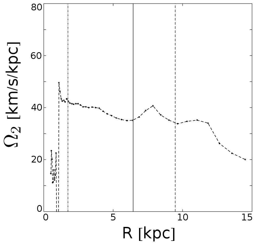
Figure 4: The $m=2$ mode pattern speed $\Omega_{2}(R)$ for the snapshot $t=1.625$ Gyr. The bar pattern speed is estimated as the mean value of $\Omega_{2}(R)$ in the interval $2.5\mbox{kpc}\leq R\leq 4\mbox{kpc}$. The inner and outer dashed vertical lines mark the position of ILR and OLR. The solid vertical line marks the position of co-rotation (CR).

Having fixed $\Omega_{bar}$ we compute the unstable Lagrangian points $L_{1}$ and $L_{2}$ in the Hamiltonian (5). Since we use the full N-body potential, the Lagrangian points are not found at exactly symmetric positions with respect to the disc’s center, while their Jacobi energies have also a small difference $2|E_{J,L1}-E_{J,L2}|/|E_{J,L1}+E_{J,L2}|\approx 10^{-4}$. Similar differences hold for the stable Lagrangian points $L_{4}$ and $L_{5}$. We finally use the information of the Lagrangian points to compute the apocentric manifold spirals emanating from the co-rotation zone. Depending on the choice of Jacobi energy, each orbit of the PL1 or PL2 families yields a different apocentric manifold. To end up with just one (representative) manifold calculation per family, we compute first the orbits PL1 and PL2 for various Jacobi energies, and keep, in each case, the orbit with Jacobi energy midway between the energies at $L_{1,2}$ and $L_{4,5}$, i.e., $E_{J,PL1}=(E_{J,L1}+E_{J,L4})/2$, $E_{J,PL2}=(E_{J,L2}+E_{J,L5})/2$. These energies roughly correspond to the median of the Jacobi energy distribution for the N-body particles in the corotation zone. The apocentric unstable manifolds of the corresponding orbits PL1 and PL2 are then computed, taking an initial segment on the apocentric surface of section with N=10000 initial conditions distributed according to $\phi_{j}=\phi_{0,PL1}-j\Delta\phi/N$, $p_{\phi,j}=p_{\phi,0,PL1}+j\Delta p_{\phi}/N$, for the outer branch, and $\phi_{j}=\phi_{0,PL1}+j\Delta\phi/N$, $p_{\phi,j}=p_{\phi,0,PL1}-j\Delta p_{\phi}/N$ for the inner branch of ${\cal W}^{UA}_{PL1}$, with $\Delta\phi$ adjusted around a value $\approx 10^{-3}$ so as to give comparable lengths for all computed manifolds, while $\Delta p_{\phi}=S_{u}\Delta\phi$, where $S_{u}$ is the slope of the unstable eigendirection of the the monodromy matrix at the fixed point PL1 (and similarly for the orbit PL2).

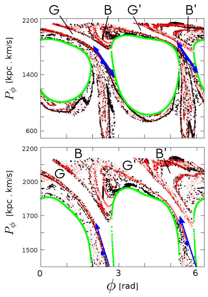
Figure 5: The apocentric surface of section as defined in Eq.(10) for the energy $E_{J}=0.5(E_{J,L1}+E_{J,L4})$, at the snapshot $t=1.625$ Gyr. The orbits in this surface of section are strongly chaotic. The bottom panel is a magnification of the top panel in the region of angular momenta $p_{\phi}$ close to the value at corotation. The black thick points are the iterates of orbits with initial conditions taken at various locations within the chaotic domain. The red points show the the apocentric invariant manifolds ${\cal W}^{UA}_{PL1,2}$. They emanate from the Lyapunov periodic orbits PL1 and PL2 shown as two blue fixed points (left and right respectively). The thick blue arrows indicate the corresponding unstable eigendirections. The closed green thick curves are limiting curves inside which the orbits are energetically forbidden. The marked features $B,B^{\prime}$ and $G,G^{\prime}$ are the ‘bridges’ and ‘gaps’ (see text).

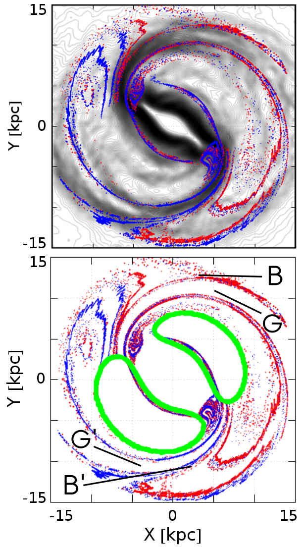
Figure 6: Top: the apocentric manifolds ${\cal W}^{UA}_{PL1}$ (red) and ${\cal W}^{UA}_{PL2}$ (blue) superposed to the ‘Sobel-Feldman’ image of the disc at $t=1.625$ Gyr. Besides the spirals, the manifolds reproduce several secondary patterns in the disc beyond the bar, such as ‘gaps’, ‘bridges’, ‘rings’ and ‘bifurcations’ of secondary spiral arms (see text for details). Bottom: the apocentric manifolds together with the limiting curves of the apocentric surface of section (green), and with the bridges and gaps marked as in the corresponding surface of section of Fig. 5.

Figure 5 shows the form of the apocentric surface of section (plane $(\phi,p_{\phi})$), as well as the apocentric manifolds of the PL1 and PL2 orbits, at the snapshot $t=1.625$ Gyr. The manifolds (red points) emanate as straight lines starting from the fixed points corresponding to the periodic orbits PL1 and PL2, but they soon develop a very complicated form, characterized by a number of thin lobes forming a ‘chaotic tangle’, which is the signature of homoclinic dynamics. Taking segments of initial conditions in the interior of the manifolds defined by the lobes marked $B,B^{\prime}$, we iterate these chaotic orbits (black points), and find that the distribution of the iterates covers more and more uniformly the area inside the manifolds’ lobes.

All together, the phase portrait formed at the indicated level of energies (Jacobi constant $E_{J}=0.5(E_{J,L1}+E_{J,L4})$) has considerable chaos. Chaos can be partly due to numerical effects, (e.g. the ‘microchaos’ generated by noise in the potential computation), but it is also of dynamical origin, due to the strong bar and spiral amplitudes. In fact, while chaos fills a substantial part of the phase space at corotation already in models with strong bars (see, for example, Patsis et al. (1997)), the deformation of all phase space structures due to the spiral mode is evident in Fig. 5. This deformation affects the form of the closed limiting curves in the apocentric surface of section, inside which the motion is energetically forbidden. These curves are found by locating the pairs $(\phi,p_{\phi})$ for which the effective potential satisfies the relation

$$\Phi_{\rm eff}(R_{c};\phi,p_{\phi})={p_{\phi}^{2}\over 2R_{c}^{2}}-\Omega_{bar}p_{\phi}+\Phi(R,\phi)=E_{J}$$ (14)

where $R_{c}$ is the root of the equation $\partial\Phi_{eff}/\partial R=0$. The above limiting curves are similar in shape to the usual curves of zero velocity, but provide the most stringent limits for the apocentric surface of section (see Tsoutsis et al. (2009).

In Fig. 5 the manifolds’ lobes from PL1 and PL2 encircle the corresponding limiting curves. However, despite the lack of energetic barrier, we observe that the uppermost manifold lobes do not fill the whole area around the limiting curves, but perform a number of oscillations leaving narrow gaps, denoted $G,G^{\prime}$, in the surface of section. This behavior of the manifolds is dictated by basic rules of dynamics, which assert that the manifold lobes of the same or different periodic orbits cannot intersect each other. In this way, we observe that the lobes of the manifold emanating from PL2 approach the manifold emanating from PL1 in the area marked $B$, but do not intersect it, leaving instead a gap $G$. Similarly, the lobes of the manifold from PL1 approach the manifold from PL2 in the area $B^{\prime}$, leaving a gap $G^{\prime}$. These features have a specific morphological correspondence in physical space, as shown below. Let us note also that the level of Jacobi energy of the surface of section in Fig. 5 is close to the median of the entire distribution of the simulation’s particles in chaotic orbits, which is consistent with the general expectation that most particles supporting chaotic spirals should be distributed in the interval of energies between $E_{J,L1}$ and $E_{J,L4}$ (Patsis (2006); Tsoutsis et al. (2008))).

Figure 6 shows, now, the main result regarding the comparison between the disc morphology and the apocentric manifolds at the snapshot $t=1.625$ Gyr. The Sobel-Feldman image of the N-body disc shows a nearly bi-symmetric set of spirals, along with secondary ring and spiral features beyond the bar. The gaps $G$ and $G^{\prime}$ appear as narrow zones separating the manifolds at the bridges $B$, $B^{\prime}$. In these bridges, the manifold emanating from the region of $L_{1}$ approaches, in a nearly-tangent direction, the exterior side of the manifold emanating from the region of the Lagrangian point $L_{2}$, and vice versa. The approach takes place via several oscillations of the manifolds in space, forming patterns recognized in the plot as bundles of preferential directions occupied by the manifolds. Such bundles mostly form spiral patterns, while breaks, or ‘bifurcations’, are also observed, splitting in two some of these bundles. Most notably, the main morphological features of the apocentric manifolds have counterparts in the Sobel-Feldman image of the real patterns formed by the disc particles.

As a final remark in this section, the manifolds ${\cal W}^{UA}_{PL1}$ and ${\cal W}^{UA}_{PL2}$ exhibit some lopesidedness, manifest also in the form of the limiting curves of the apocentric surface of section as projected in physical space. This effect implies that the outflow of particles in chaotic orbits, in the directions indicated by the manifolds, is not symmetric with respect to the disc center. Since the phase space outside corotation is open to escapes, particles escaping in chaotic orbits carry with them linear momentum in a distribution of orientations non-symmetric with respect to the center. The contribution of this to maintaining a disc-halo ‘off-centering effect’ is discussed in subsection 4.3.

4 Secular evolution

In this section we focus on how the various spiral and other non-axisymmetric features beyond the bar evolve along with the bar’s secular evolution. We also examine which mechanisms are responsible for the maintainance of appreciable levels of non-axisymmetric activity. In the end of the section we return to the comparison between manifolds and the observed patterns in the disc (as in Fig. 6), but for different snapshots covering the whole disc’s secular evolution.

4.1 Bar spin-down

A basic manifestation of secular evolution is the bar’s spin down, as shown in Fig. 7, which leads to a an outward slow displacement of the ILR, CR and OLR. Thus, $(R_{ILR},R_{CR},R_{OLR})\simeq(1.75,6.5,9.5)$ kpc immediately after the bar formation and $(3.1,7.5,12)$ kpc at the end of the simulation. The bar’s spin down can be associated with several factors, as for example: i) particles abandoning the bar and carrying angular momentum outwards at incidences of growing spirals (see below), or ii) transfer of angular momentum to the halo (see Debattista & Sellwood (1998); Debattista & Sellwood (2000); Athanassoula (2002); Athanassoula & Misiriotis (2002); Athanassoula (2003)).

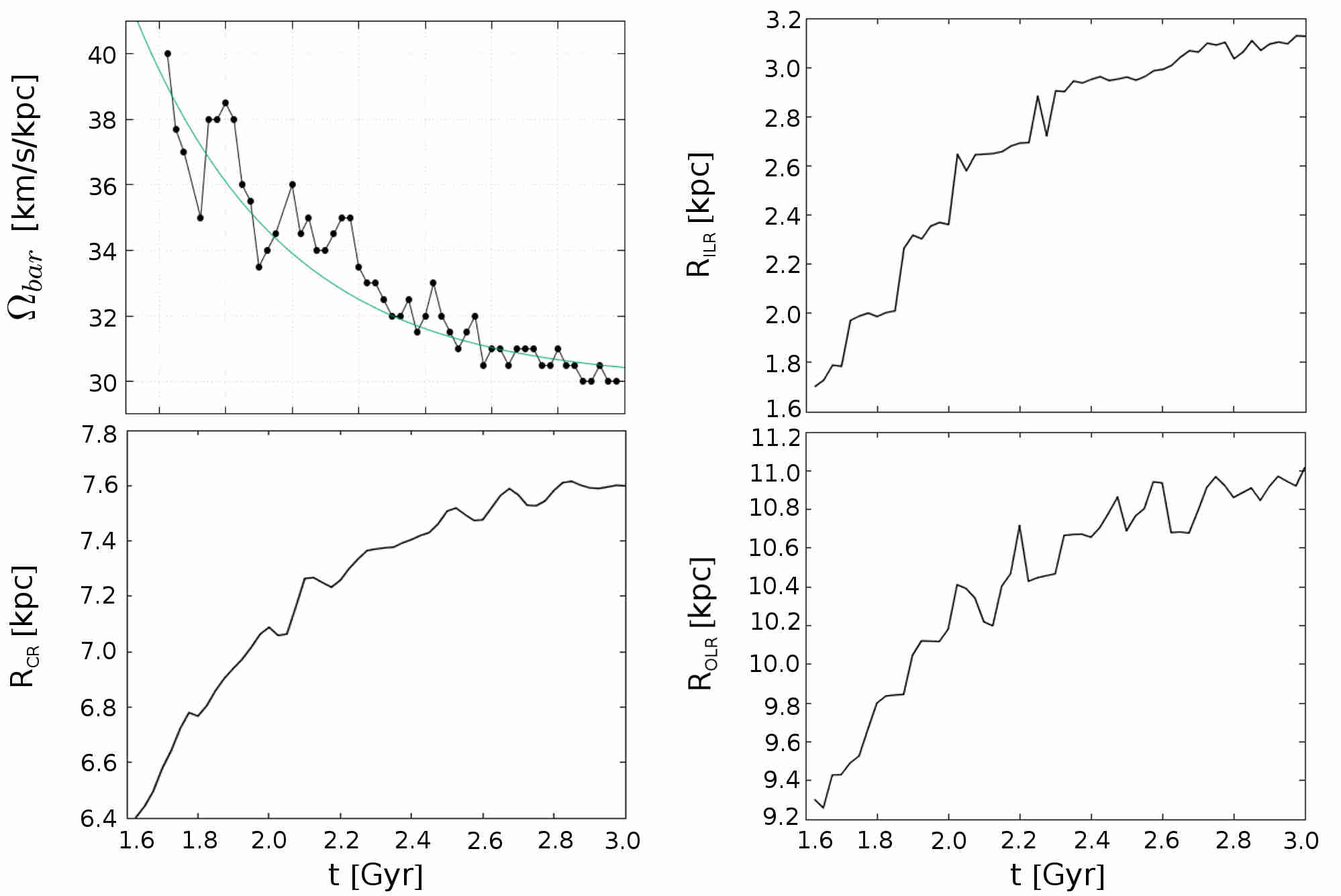
Figure 7: Top left: Evolution of the bar’s pattern speed. The cyan curve represents an exponential fitting $\Omega_{bar}(t)=\Omega_{0}-\Omega_{1}\left(1-\exp\left(-{t-t_{0}\over t_{d}}\right)\right)$, with $\Omega_{0}=42$ km/sec/kpc, $\Omega_{1}=11$ km/sec/kpc, $t_{0}=1.625$ Gyr, $t_{d}=2$ Gyr. The remaining panels show the evolution of the radii of the bar’s ILR (top right), CR (down left), and OLR (down right).

The bar retains high amplitudes throughout the simulation. Thus, whereas slowing down, the bar sustains appreciable levels of orbital chaos in the disc. Figure 8, top panel, shows the evolution of the distribution of the disc particles’ Jacobi energies, along with more phase portraits at energies, or snapshots, different from the one of Fig. 5. The distribution of Jacobi energies evolves by keeping its global maximum always close to the instantaneous CR value, hence it is shifted towards absolutely smaller energies as the bar slows down. The dispersion of the Jacobi energies is also reduced in time, but remains at a level of few times $10^{4}km^{2}/s^{2}$. The remaining panels in Fig. 8 show apocentric surfaces of section selected so as to cover the entire range of energies where particles are practically distributed, for $t=1.65$ Gyr (as in Fig. 5) and at a later snapshot $t=2.425$ Gyr. Similar phase portraits are found in all snapshots. Chaos is ubiquitous in all these portraits, indicating that the spiral and other structures beyond the bar are supported mostly by chaotic orbits.

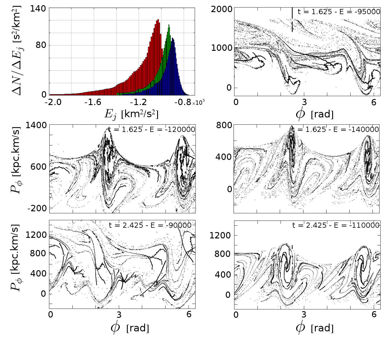
Figure 8: Top left: Evolution of the distribution of the Jacobi energies of the disc particles at the snapshots $t=1.625$ Gyr (red), $2.05$ Gyr (green), and $2.425$ Gyr (blue). In comparison, the jacobi energies at CR are (in $km^{2}/s^{2}$), $E_{J}=-1.05\times 10^{5}$, $-0.94\times 10^{5}$ and $-0.91\times 10^{5}$ respectively. The top right and middle panels show the apocentric surfaces of section for the snapshot $t=1.65$ Gyr, in energies different from the one of Fig. 5, selected to cover the range of the corresponding distribution. The bottom panel shows two surfaces of section for the snapshot $t=2.425$. Chaos is ubiquitous in all these plots.

4.2 Incidents of spiral and other non-axisymmetric activity

The variability of the bar, spiral and other non-axisymmetric patterns is reflected in time variations of the Fourier amplitude $C_{2}(R)$, as shown in Figure 9, top panel, for different radii. The group of curves for $R=3,4$ and $5$ kpc quantify the evolution of the bar’s strength. The bar reaches its maximum strength near $t=1.6$ Gyr, leading to a $m=2$ amplitude larger than unity. Thereafter, the bar $m=2$ amplitude stabilizes in the interval from $t=1.6$ to $t=2.1$ Gyr. After a small but abrupt drop at $t=2.1$, associated with the buckling instability, the bar’s amplitude slowly decays through the remaining $~{}2$ Gyr of the simulation, remaining however always of order of unity.

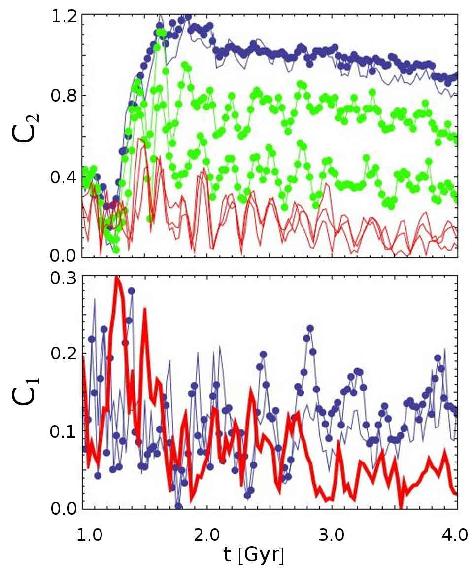
Figure 9: Top: evolution of the Fourier amplitude $C_{2}$ in the interval $1\leq t[Gyr]\leq 4$. The value of $C_{2}$ is shown at the distances $R=3,4$ kpc (dotted blue), $R=5$ kpc (solid line, blue), $R=6,7$ kpc (dotted green), and $R=8,9,10$ kpc (solid red). Bottom: evolution of the Fourier amplitude $C_{1}$ at $R=3$ kpc (dotted blue), $R=4$ kpc, (solid blue), and $R=12$ kpc (thick solid red).

The increase and subsequent slow decay of the $m=2$ bar mode permeates all radial annuli across the disc. The $m=2$ amplitude in general falls with $R$ between CR and OLR, but it tends to stabilize to a mean level $\sim 0.2$ in an annulus $8\leq R[kpc]\leq R_{OLR}$. The amplitude $C_{2}$ undergoes oscillations which are nearly in-phase for all radii within this annulus. At local maximum of these oscillations $C_{2}$ exceeds 0.2, up to $t\sim 3$ Gyr, while the oscillations are milder afterwards. At all peaks of the $C_{2}$ mode in the interval $1.5\leq t[Gyr]\leq 4$ we observe ‘incidents’ of non-axisymmetric activity in the outer parts of the disc. Taking the mean $C_{2}$ from the three lowermost curves in the top panel of Fig. 9, we estimate the times when such incidents reach maximum amplitude (to a precision related to the frequency of saving of the particles’ positions, i.e., every 25 Myr). We thus identify the following sequence of times:

$$t[Gyr]^{(incident)}=1.625,1.8,1.95,2.2,2.375,2.525,$$

$$2.725,2.950,3.1,3.325,3.75,3.95.$$ (15)

By the above sequence, an approximate period $T\approx 0.2$ Gyr can be deduced, but with large fluctuations $\Delta T\sim 0.1$ Gyr. The bar has a pattern speed $\Omega_{bar}\approx 40$ Km/sec/kpc (period $T_{bar}\approx 0.15$ Gyr) at the starting time and $\Omega_{bar}\approx 30$ Km/sec/kpc ($T_{bar}\approx 0.2$ Gyr) at the end of the sequence. Thus, the sequence (4.2) is in rough resonance with the bar’s rotation. However, the bar itself exhibits some extra phenomena. The bottom panel of Fig. 9 show important oscillations in the $m=1$ mode at disc radii smaller than the bar’s half-length. In these oscillations $C_{1}$ reaches a mean level $\sim 0.1$, with peaks up to $\sim 0.3$, and an approximate period $T\sim 0.4$ Gyr in the interval from $t=2$ Gyr to $t=3$ Gyr. Oscillations of $C_{1}$ appear also in the outer disc, albeit not in phase with those of the inner disc.

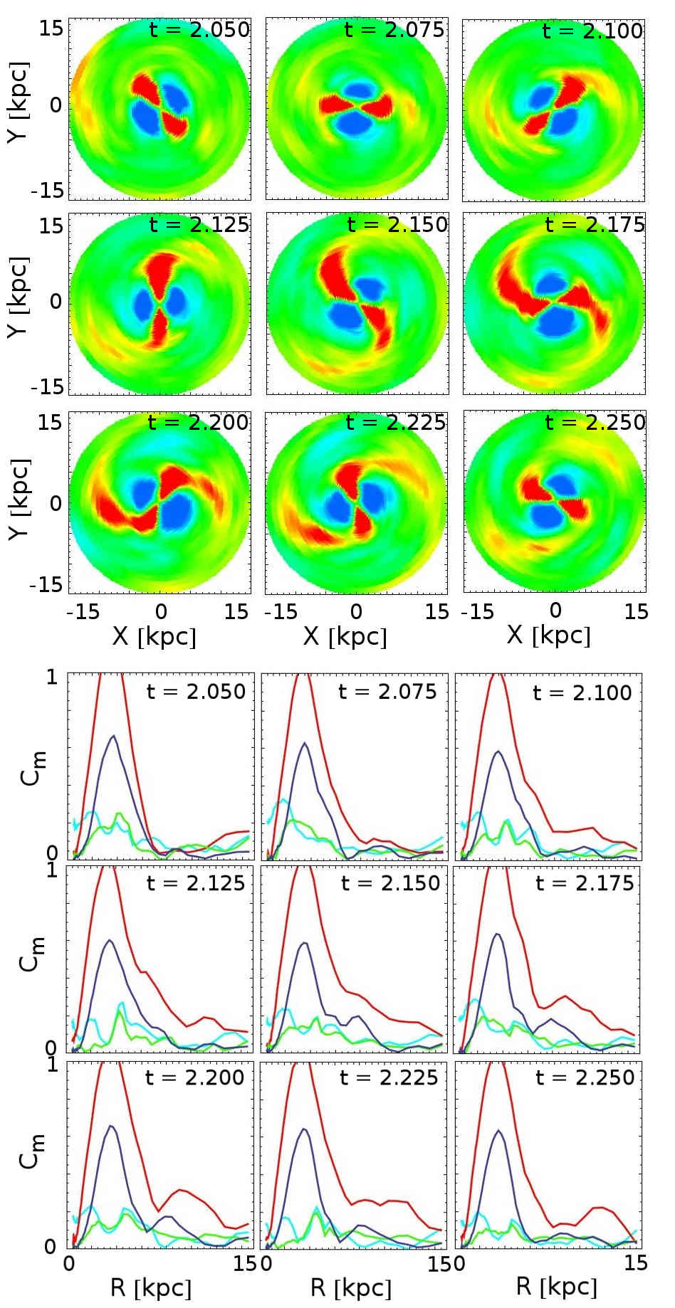
Figure 10: Top: an ‘incident of inner origin’, whose corresponding $C_{2}$ maximum occurs around $t=2.2$. Bottom: the Fourier amplitudes $C_{m}(R)$ for $m=1$ (cyan), $m=2$ (red), $m=3$ (green), and $m=4$ (blue). The dotted vertical line marks the position of the bar’s CR. An $m=2$ disturbance propagates from CR outwards. Significant rise of the $m=1$ and $m=3$ modes appears inside the bar at the initial phase of the incident.

Through density excess maps, and the corresponding profiles of the Fourier modes $m=1,2,3,4$, we can see how incidents of non-axisymmetric activity affect the disc’s morphology beyond the bar. We distinguish two types of incidents, exemplified in Figs.10 and 11 respectively, as follows:

-Incidents of inner origin: an incident of inner origin corresponds morphologically to a spiral wave emanating from the end of the bar, and travelling outwards, until it becomes detached from the bar. An example is given in Fig. 10, showing the density excess maps at nine snapshots around the time $t=2.2$, which belongs to the sequence (4.2). The outwards ‘emission’ of the spiral wave from the bar becomes evident after $t=2.15$ Gyr. At earlier times, one observes the appearance of small leading extensions of the bar, so that the whole incident is reminiscent of swing amplification. The creation of a leading component can be associated with flow of material approaching the bar from the leading direction by moving along outer families of periodic orbits such as the 2:1 family (Patsis; private communication). The spirals start fading out after detaching from the bar.

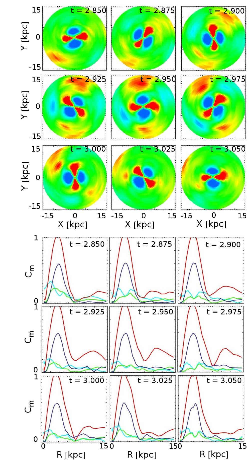
Figure 11: Same as in Fig. 10, but for an incident of outer origin reaching its peak around $t=2.95$. An $m=2$ disturbance generated in the outer parts of the disc is reflected at CR. Significant rise of the $m=1$ and $m=3$ modes appears again inside the bar.

- Incidents of outer origin: an incident of outer origin corresponds morphologically to a rise of the surface density excess in the outer parts of the disc, as shown in Fig. 11. The rise appears both in the $m=1$ and $m=2$ modes. The left panels in Fig. 11 indicate that the $m=2$ perturbation arises at radial distances beyond $R=12$ kpc, it travels inwards, and then it is reflected at corotation. It is stressed that these features are not connected with the present analysis of spirals based on manifolds. However, they may contribute to other effects observed in the disc as discussed below.

Figure 12 shows the density excess map of the disc for all times of the sequence (4.2). Incidents of inner origin appear at the snapshots $t=1.625$, $t=1.95$, $t=2.2$, $t=2.725$ Gyr, while incidents of outer origin appear at $t=2.375$, $t=2.95$, $t=3.75$, and $t=3.95$ Gyr. A classification as inner or outer is unclear for the incidents taking place at $t=1.8$, $t=2.525$, $t=3.1$, and $3.325$ Gyr. Incidents of inner origin appear mostly in the interval $1.6<t[Gyr]<3$, while incidents of outer origin are observed throughout the simulation. In fact, the disc becomes overall less responsive to non-axisymmetric perturbations as the time goes on, and a transition from stronger to weaker incidents is discernible around $t\approx 3$ Gyr.

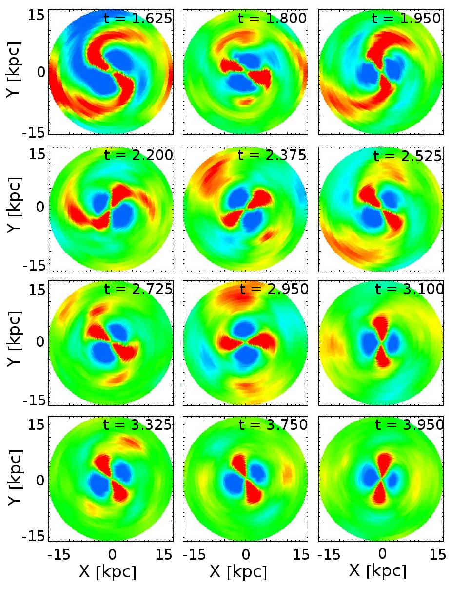
Figure 12: Non-axisymmetric density excess maps showing the peaks of the ‘incidents’ of non-axisymmetric activity for all snapshots of the sequence of Eq. (4.2).

4.3 Relative disc-halo orbit and its effect on the disc

At every inner incident of spiral activity, the particles’s orbits change as the potential develops rapid fluctuations. This is accompanied by changes in the particles’ energies and angular momenta. Figure 13 summarizes these effects. We consider moving time windows $W(t)=(t-\Delta T_{w}/3,t+2\Delta T_{w}/3)$ with $\Delta T_{w}=0.125$ Gyr, as well as an annulus $R_{min}\leq R\leq R_{max}$, with $R_{min}=5$kpc and $R_{max}=18$ kpc, equal to six disc exponential scale lengths. At a snapshot $t$ we isolate all particles whose orbits have crossed both limits of the annulus within the time window $W(t)$. We finally collect these particles for all time windows, and check their orbits. This process collects about 10% of the disc particles whose orbits behave as above at least in one time window. Figure 13, top, shows $R(t)$ for a sample of 100 randomly chosen trajectories in this set. Analogous pictures are obtained for any other random choice. Note that the N-body code represents forces sufficiently smoothly to produce smooth particle orbits. The main feature of these orbits is their change of elongation (difference between apocenter and pericenter) in different time windows. Abrupt changes are observed for some orbits at particular times, connected to an abrupt change in the angular momentum (middle panel). These times correspond to the growth phase of major incidents of non-axisymmetric activity in the disc. Τhe effect is more notorious for the first incident of spiral growth a little before $t=0.5$ Gyr (before the bar), as well as the growth of the manifold spirals at $t=1.5$ and $t=1.65$ Gyr. In every incident the majority of affected orbits become more elongated after the incident than before (although both types or orbital changes are observed). Also, the majority of affected orbits exhibit increase of the angular momentum, which mostly affects an orbit by increasing its apocentric distance to a large value (more than 20 kpc for some particles in Fig. 13), while many particles move also to orbits with pericentric distance beyond co-rotation.

The relative influence of each incident in the orbits can be estimated by measuring the fraction $\Delta N_{esc}(t)/N_{esc}$, where $N_{esc}$ is the total number of particles which, in at least one time window exhibited a crossing of the annulus $R_{min}\leq R\leq R_{max}$ as described above, and $\Delta N_{esc}(t)$ is the number of particles doing so in the time window $W(t)$. The bottom panel in Fig.13 shows the evolution of $\Delta N_{esc}(t)/N_{esc}$ for four choices of $R_{max}$, namely $R_{max}=12,14,16$ and $18$ kpc. Consecutive ‘incidents’ of non-axisymmetric activity cause an oscillatory behavior of these curves. For nearly all particles in the population $N_{esc}$ the first event is associated with the growth of the bar (at $t=1.4$ Gyr), while for most particles (up to a percentage $80$%) we have repeated events associated with the growth of the manifold spirals at $t=1.5$, $t=1.65$ and $t=1.8$ Gyr. Smaller percentages appear at subsequent times, as the incidents of non-axisymmetric activity beyond the bar slowly decay in amplitude.

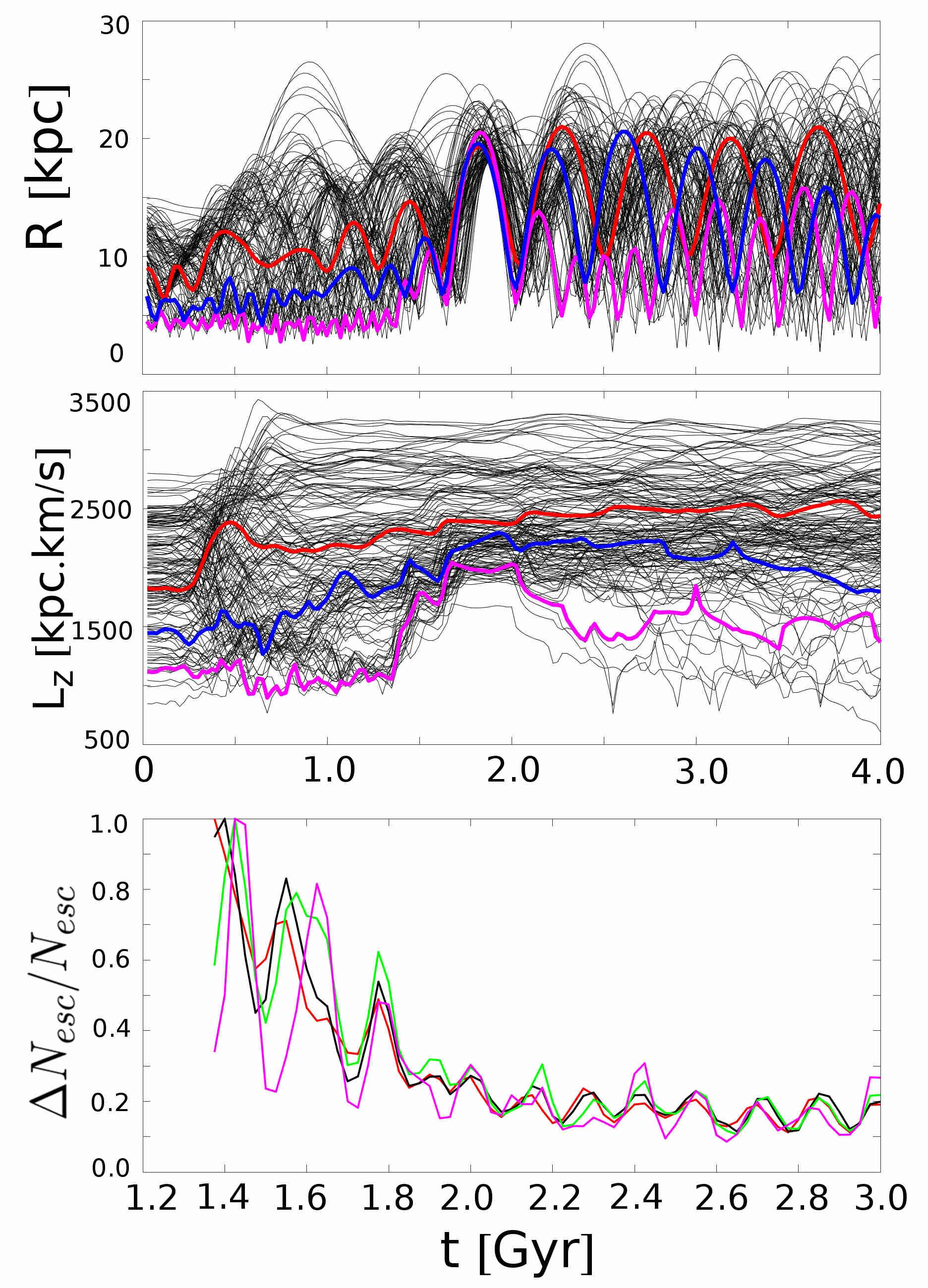
Figure 13: Top: evolution of the radius $R$ for one hundred randomly selected particles whose orbits cross the annulus $R_{min}\leq R\leq R_{max}$ in at least one time window $W(t)$ (see text). The colored curves show three different types of behavior, namely, a gradual increase of the apocenter (red), an increase taking place mostly in isolated ‘incidents’ (blue), and an orbit going to a larger and then returning to a smaller apocenter (purple). Middle: evolution of the angular momentum per unit mass $L_{z}=p_{\phi}$ for the same particles. Bottom: the relative fractions $\Delta N_{esc}(t)/N_{esc}$ (see text) when $R_{max}$ is taken equal to $12$ kpc (red), $14$ kpc (black), $16$ kpc (green), $18$ kpc (purple).

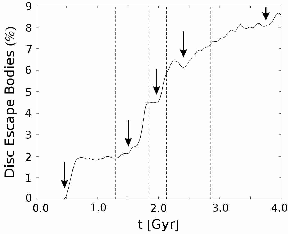
Figure 14: Percentage of disc particles found at a distance $R>R_{esc}=18$ kpc, as a function of time. The arrows indicate times when an abrupt increase of escaping disc particles is observed. The dashed vertical lines correspond to the limits of time intervals ($t_{1}$ to $t_{4}$) in which the relative disc-halo orbit is observed to change character, i.e., to switch from circumcentric to epicyclic, and vice versa (see text).

The orbital changes observed at major incidents of non-axisymmetric activity result in a increase in time of the percentage of disc particles beyond any sufficiently large radius $R$. The increase is statistical, since it is due both to particles really escaping the system or ones moving in bounded, but elongated orbits, being pushed, however, outside co-rotation. We conventionally call the radius $R=R_{esc}=18$ kpc as the ‘escape’ radius, and the particles found at $R>R_{esc}$ at the time $t$ ‘escape bodies’. Figure 14 shows the evolution of the percentage of ‘escape bodies’ $\Delta N_{esc}/N_{disc}$. The contribution of major incidents of non-axisymmetric activity is identified in this plot as an abrupt increase of $\Delta N_{esc}/N_{disc}$. Three major events are observed to take place at the times $t=0.55$, $t=1.7$ and $t=2.1$ Gyr, while smaller ones at the times $t=2.5$ and $t=2.9$ Gyr. Besides the first event at $t=0.55$ (before the bar), the remaining ones are all associated with incidents of inner origin. Outer incidents may also affect the particles’ orbits, but their influence on $\Delta N_{esc}/N_{disc}$ should be smaller, as the corresponding disc disturbances propagate inwards and then outwards (being reflected at CR, see above).

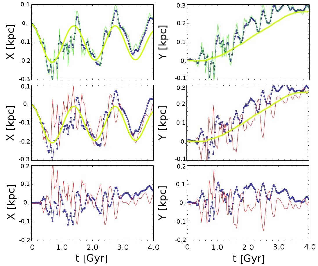
Figure 15: Top row: Time evolution of the $x-$coordinate (left), and $y-$coordinate (right) of the center of mass of the halo particles (blue dotted) or the bulge particles (cyan solid line). The thick green line shows the corresponding evolution of the $x-$ and $y-$ co-ordinates of the total center of mass of all particles included in the simulation box. Middle row: same as in the top row but for the centers of mass of the halo particles (blue-dotted) and the disc particles (red solid). Bottom row: Relative orbits of the halo (blue dotted) and disc (red solid) centers of mass with respect to the center of mass of the total system.

Assuming, now, that the particles connected with these events move in chaotic orbits, one expects important fluctuations in the number of particles escaping co-rotation as a function of the final direction in which the particles move. As a result, the main body of the disc recoils in a direction changing stochastically in time, the effect being larger at times connected with major incidents. This recoil sets the main body of the disc in relative orbit with respect to the spheroid components (i.e. bulge+halo). Figure 15 illustrates the phenomenon. We compute the evolution of the position of the center of mass $\mathbf{r}_{cm}^{(d)}(t)$, $\mathbf{r}_{cm}^{(b)}(t)$, $\mathbf{r}_{cm}^{(h)}(t)$, for the disc, bulge and halo components respectively. For the disc particles we use an iterative algorithm to specify the center of mass of only those particles characterized as ‘non-escaping’. Namely, we first compute the center of mass $\mathbf{r}_{cm}^{(d,0)}$ of all disc particles, and then consider the center of mass of only those disc particles satisfying $R<R_{esc}$, where $R$ is the cylindrical radial distance of a particle with respect to $\mathbf{r}_{cm}^{(d,0)}$. Alternative ways to compute $\mathbf{r}_{cm}^{(d)}$, taking the center of the computational box or the center of mass of the total system as origin, yield practically indistinguishable results. Finally, we compute the time evolution of the center of mass of all bodies in the simulation $\mathbf{r}_{cm}^{(all)}$. In a perfect momentum-preserving scheme, the vector $\mathbf{r}_{cm}^{(all)}$ should remain constant in time (the net total momentum in the simulation initially vanishes). However, very slow smooth variations of the global center of mass are obtained as a result of the use of adaptive mesh-refinement as well as the fact that the accelerations of particles escaping the computational box are computed with multipole formulas instead of cloud-in-cell interpolation (see Kyziropoulos et al. (2017a) for details). These phenomena are a priori predictable, and they cause the global center of mass to undergo a smooth slow displacement with time-varying velocity not exceeding the value $0.3$ Km/sec in any of its three Cartesian components during the whole simulation (thick solid curves in top and middle panels of Fig. 15). On the other hand, the main effect to be observed in the same figure is that each of the three individual components $\mathbf{r}_{cm}^{(d)}(t)$, $\mathbf{r}_{cm}^{(b)}(t)$, $\mathbf{r}_{cm}^{(h)}(t)$ undergo rapid stochastic variations around the global center of mass. We checked that such variations are important only in the projections of the three vectors on the disc plane, and they can be described as follows: The $x-$ and $y-$ components of the centers of mass of the halo and bulge undergo rapid stochastic variations around the smooth curves $x^{(all)}(t)$, $y^{(all)}(t)$, remaining, nevertheless always closely attached to each other. On the contrary, the $x-$ and $y-$ components of the vector of the disc center of mass exhibit rapid fluctuations which set the disc in relative orbit with the (nearly coinciding) centers of mass of the halo-bulge.

The evolution of the relative orbit of the halo-bulge, and disc with respect to the global center of mass $\mathbf{r}_{cm}^{(all)}$ is shown in the bottom panel of Fig. 15 ($x,y$ components of $\mathbf{r}_{cm}^{(h)}(t)-\mathbf{r}_{cm}^{all}(t)$ and $\mathbf{r}_{cm}^{(d)}(t)-\mathbf{r}_{cm}^{all}(t)$). The separation between disc and halo-bulge increases near major incidents of non-axisymmetric activity, and the group of spheroidal components (halo-bulge) is set in relative motion with respect to the disc. The first major separation takes place near $t\approx 0.3$ Gyr (first major growth of spirals before the bar). After the bar is formed, it is unclear whether the bar’s center of mass moves closer to the rest of the disc or to the spheroid (halo-bulge). We keep the conventional separation of the system into disc and spheroid (halo-bulge) components, hereafter referred to as the ‘relative disc-halo’ orbit $\mathbf{\Delta r}_{hd}(t)\equiv\mathbf{r}_{cm}^{(h)}(t)-\mathbf{r}_{cm}^{(d)}(t)$. The disc-halo orbit is depicted in Fig. 16, starting from the time $t=1.4$ Gyr, immediately after the first incident of spiral activity accompanying bar formation. The four panels correspond to intervals in which the relative disc-halo orbit changes character, i.e., from ‘circumcentric’ (described around the disc center) the orbit switches to ‘epicyclic’ (the halo-bulge center of mass describes one or more small epicycles with respect to the disc center), and vice versa. These switches take place at the times $t_{1}=1.4$ Gyr, $t_{2}=1.825$ Gyr, $t_{3}=2.125$ Gyr, and $t_{4}=2.95$ Gyr. The first ‘epicyclic’ interval is rather short ($t_{3}-t_{2}=0.325$ Gyr), while the second is longer ($t_{4}-t_{3}=1.05$ Gyr) and within it the relative disc halo separation tends to zero, leading the whole system again close to a state of common center of mass of all components. Most notably, the times $t_{1}$, $t_{2}$, $t_{3}$ and $t_{4}$ differ by $~{}0.2-0.3$ Gyr, from the times when abrupt changes in $\Delta N_{esc}/N_{esc}$ take place in Fig. 14. The time difference is of the order of one radial orbital period for the particles of Fig. 13. We regard these facts as evidence that the orbital switches observed in Fig. 16 are connected with the disc recoil effect.

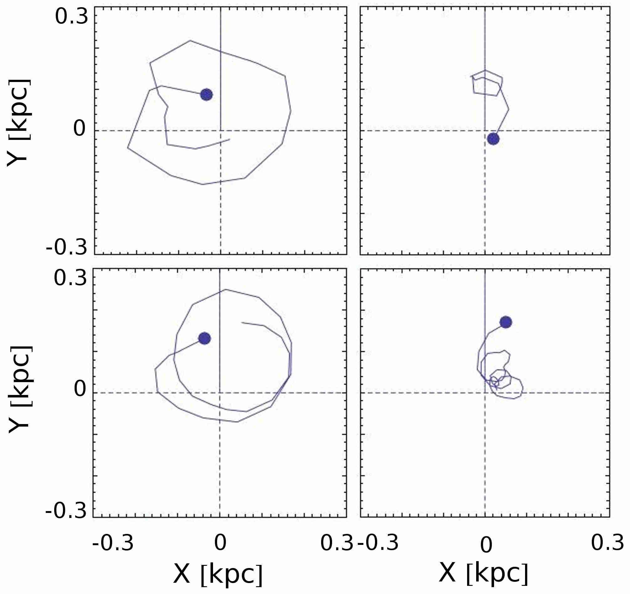
Figure 16: The relative orbit of the spheroid (halo-bulge) center of mass with respect to a non-inertial observer centered at the disc center of mass (components $y$ vs. $x$ of the vector $\mathbf{\Delta r}_{hd}(t)$) at four time intervals $(t_{1},t_{2})$ (top left), $(t_{2},t_{3})$ (top right), $(t_{3},t_{4})$ (bottom left), and $(t_{4},4\mbox{Gyr})$ (bottom right), with $t_{1}=1.4$ Gyr, $t_{2}=1.825$ Gyr, $t_{3}=2.125$ Gyr, $t_{4}=2.95$ Gyr.

The relative disc-halo orbit shown in Fig. 16 is quite small compared to the system’s scale. Fig. 17 shows the variations of $d(t)=|\mathbf{\Delta r}_{hd}(t)|$ from $t=1$ Gyr to $4$ Gyr. This interval can be split into sub-intervals representing circumcentric or epicyclic parts of the disc-halo orbit. In both cases, the distance $d(t)$ presents an oscillatory behavior, leading to a minimum distance close to $d_{min}\approx 0$ and maximum distance $d_{max}\approx 0.25$ kpc. Despite the small size of the disc-halo orbit, the displacement of the halo-bulge component with respect to the disc causes a significant $m=1$ perturbation in the disc. Using a simple model (Appendix I) we find that the amplitude of the $m=1$ perturbation scales with the separation as ${\cal O}(d/R_{d})$ at distances up to $R\sim R_{d}$, where $R_{d}$ is the disc’s exponential scale length. With $d$ as small as $\sim 0.2-0.3$ kpc and $R_{d}=3$ kpc we find an induced $m=1$ perturbation $~{}0.1$ (see Fig.22)). Figure 17 shows direct evidence of the correlation between variations of $d$ and of the relative amplitude $C_{1}$ in the disc. The correlation is strong in a domain $3\leq R[\mbox{kpc}]\leq 5$ (top panel), which contains the bar beyond its ILR, and connects maxima and minima of $d$ with maxima and minima of $C_{1}$ both in the circumcentric and epicyclic parts of the disc-halo orbit. Some change in the mean levels of both $d$ and $C_{1}$ is observed at every orbital switch. The correlation is weaker at larger radii (bottom panel). Thus, the displacement affects the disc’s inner part.

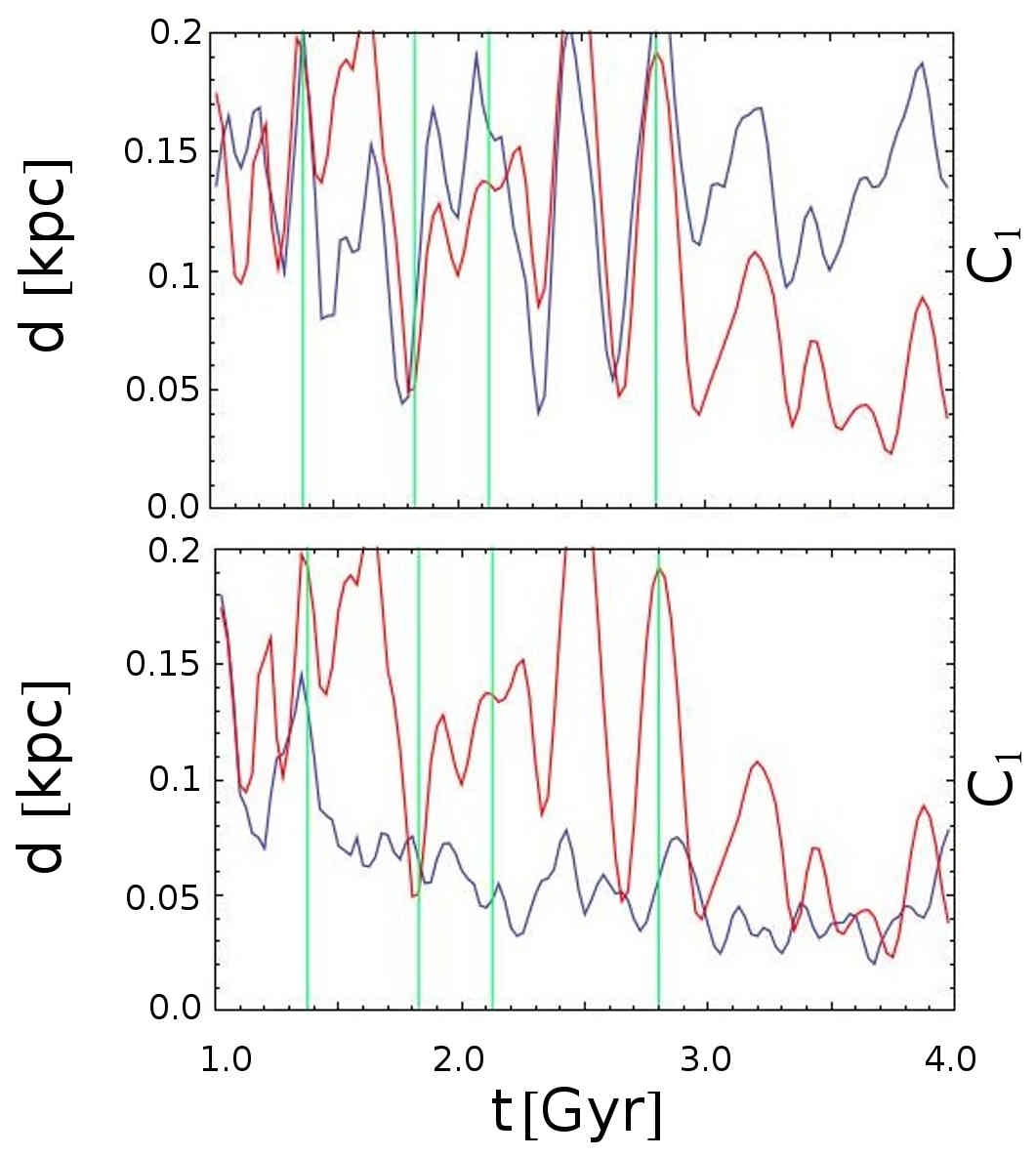
Figure 17: Top: evolution of the disc-halo displacement $d$ (red, values as in left vertical axis), compared to the mean $C_{1}$ from three values at $R=3,4$ and $5$ kpc (blue, values as in right vertical axis). The cyan vertical lines indicate the times $t_{1}$ to $t_{4}$ (same as in Fig. 16). Bottom: same as top but for the mean $C_{1}$ from three values at the radii $R=8,9$ and $10$ kpc.

The displacement causes also a direct $m=2$ effect whose size is of order ${\cal O}\left((d/R_{d})^{2}\right)$, hence much smaller than the $m=1$ effect. However, the orbital response of disc particles to the $m=1$ perturbation affects mostly particles inside the bar. Due to chaos inside co-rotation (Fig. 8), even small potential fluctuations of any harmonics largely influence the particles’ orbits. In particular, particles coming closer to the manifolds can abandon co-rotation in the direction dictated by the manifolds. This leads to an indirect $m=2$ effect. The size of the effect can be estimated by the correlations between $d$ and the disc’s $C_{2}$. Figure 18 shows that $d$ and $C_{2}$ tend to switch from anti-correlated to correlated when the disc-halo relative orbit switches from epicyclic to circumcentric. Uncertainties in this figure obstruct a clear conclusion. As additional evidence, Figs. 10 and 11 show a significant rise of the $m=1$ (and also $m=3$) component in the bar at the initial phase of the incidents of both inner and outer origin. A similar rise is observed in all major incidents.

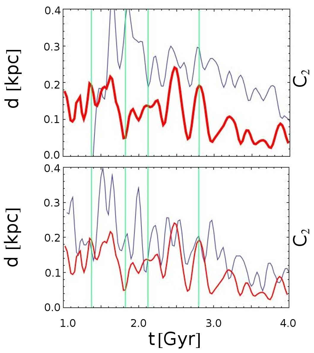
Figure 18: Same as in 17, but for the mean $C_{2}$ (blue) at the indicated distances.

4.4 Manifold spirals and the evolution of non-axisymmetric patterns in the disc

It was argued above that the manifolds act as drivers of the orbital evolution for particles in chaotic orbits pushed to move away from co-rotation. This effect is pronounced at major incidents of non-axisymmetric activity, but the role of manifolds as drivers of the orbital evolution should hold independently of the growth or decay in amplitude of such incidents. We now compare the evolution of non-axisymmetric patterns in the disc beyond the bar with the evolution of the patterns created by the manifolds, both in minima and maxima of the non-axisymmetric activity. The comparison is in terms of the shapes of these patterns.

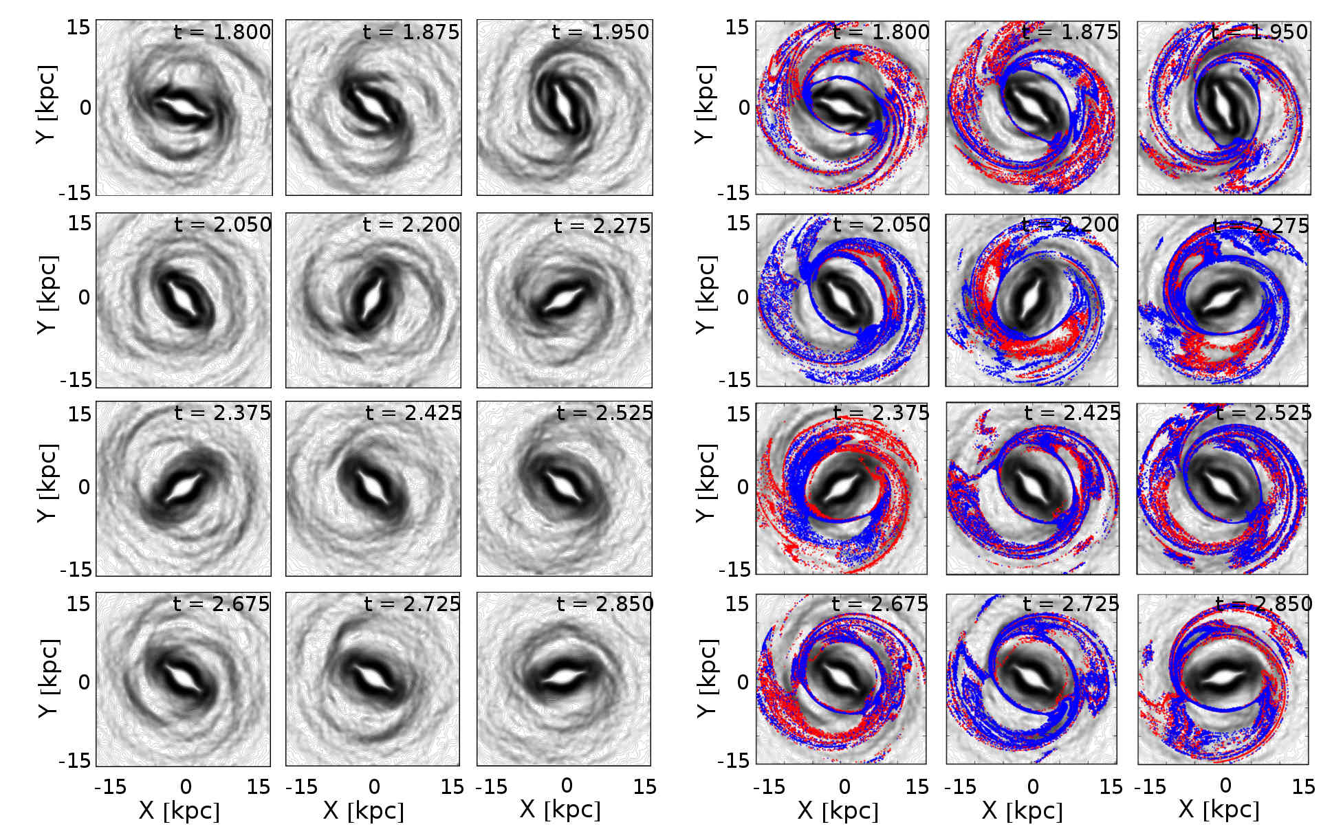
Figure 19: Left: Sobel-Feldman images of the disc in twelve snapshots corresponding to both maxima and minima of $C_{2}[9\mbox{kpc}]$ (see text). Right: the apocentric manifolds for the same snapshots (colors same as in Fig.6), superposed to the Sobel-Feldman images.

In Fig. 9, nearly in-phase oscillations of the amplitude $C_{2}$ occur in the outer parts of the disc. We focus on such oscillations in the time interval $1.8<t[\mbox{Gyr}]<2.8$ (major incidents of inner origin, connected with spiral patterns, do not appear beyond this time). To locate more precisely the times of occurence of such incidents, we choose a reference radius $R=9$ kpc which is between the bar’s CR and OLR throught the simulation. Six consecutive local maxima and six minima of $C_{2}[9\mbox{kpc}]$ occur at the times

$$t^{(max,9\mbox{\small kpc})}[\mbox{Gyr}] = 1.8,1.95,2.2,2.375,2.525,2.725$$ (16)

$$t^{(min,9\mbox{\small kpc})}[\mbox{Gyr}] = 1.875,2.05,2.275,2.425,2.625,2.85~{}~{}.$$

Figure 19, left, shows the Sobel-Feldman images of the disc in the above times, alternating between a time of maximum and a time of minimum. In a timescale as short as one bar’s period one finds a strong variability of the patterns identified in the disc beyond the bar. Note that the Sobel-Feldman algorithm allows to recover patterns which are quite fuzzy in simple surface-density processed images of the disc. In particular, some form of spiral activity is identifiable in all snapshots of Fig. 19, although the morphology of these spirals (number of arms, pitch angle, radial extent, etc) rapidly change. Besides the main spirals, other secondary features appear and disappear in succession, as, for example, rings (e.g. at $t=1.8$ and $t=2.375$ Gyr) and bifurcations of more spirals (e.g. at $t=1.95$ Gyr). Figure 19, right, shows the same images on top of which the apocentric manifolds are superposed. An overall comparison shows that the manifolds and Sobel-Feldman deduced patterns exhibit a similar level of complexity (forming, in the case of the manifolds, a ‘chaotic tangle’ Wiggins (1990); see also Voglis et al. (2006a)). Also, they agree in shape and orientation to a large extent. In more detail, however, the level of agreement varies between snapshots. A (rather subjective) visual comparison, distinguishes snapshots of better (e.g. $t=1.95,2.275$ or $2.725$ Gyr) or worse agreement (e.g. $t=2.425,2.625$ Gyr) than average. The following are some basic remarks regarding this comparison:

- The manifolds’ homoclinic lobes account for the systematic appearance of features called gaps, bridges and bifurcations in section 3. Such features appear in nearly all panels of Fig. 19, and show a counterpart in the Sobel-Feldman disc images. We note that gaps and bridges can be recognized also in several plots of ‘flux-tube’ manifods (see Athanassoula (2012)), but they are better visualized using the apocentric manifolds.

- In nearly all patterns there are small phase differences ($\leq 5^{\circ}$ between some manifold lobes and the corresponding spirals in the Sobel-Feldman image (the largest difference is found for $t=2.375$ Gyr). This might be a dynamical phenomenon (disc response has delay with respect to the manifolds), but it may also be an artefact of the visualization by the apocentric manifolds, since the disc’s local density maxima are close to, but do not necessarily coincide with the individual orbits’ apocenters (Tsoutsis et al. (2008)).

- For computational convenience, we just choose one value of the Jacobi constant for the manifold computation. The manifolds retain a rather robust pattern against changes of the Jacobi energy (Tsoutsis et al. (2008)), but small variations in shape are allowed. Most notably, besides the manifolds of the PL1 or PL2 orbits, the chaotic tangle is supported by the manifolds of all families of unstable periodic orbits in the corotation region. Superposed one on top of the other, these manifolds form amore robust spiral pattern called ‘manifold coalescence’ in Tsoutsis et al. (2008). The manifold coallesence is a better representation of chaotic dynamics in the co-rotation zone than the manifolds of any single family. Nevertheless, its computation for many snapshots is a voluminous work extending outside our present scope.

- Finally, despite the clear correlation between manifolds and Sobel-Feldman detected patterns, not all patterns in the disc need necessarily be linked to the manifolds. Structures such as outer rings or slowly rotating outer spirals may not be supported by chaotic flows, but instead, by the regular flows associated with standard density wave theory (Boonyasait et al. (2005); Struck (2015)).

4.5 Consistency with multiple pattern speeds

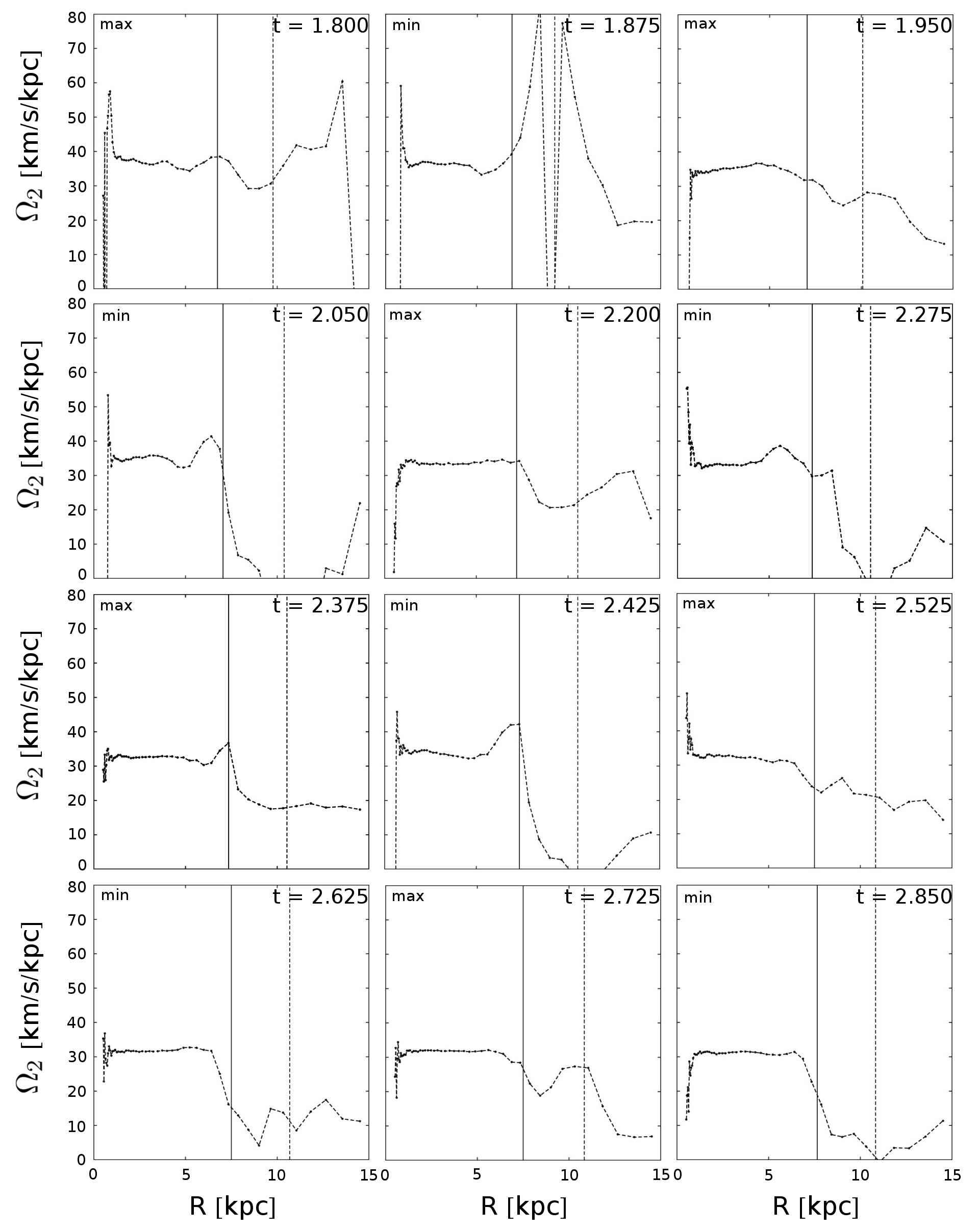
Figure 20: Profiles of the pattern speed $\Omega_{2}$ as a function of the radius $R$ from the disc center at the same snapshots as in Fig. 19. The inner plateau at distances between $2$ kpc and $4$ kpc determines the bar’s pattern speed. The two vertical lines mark the position of CR and OLR. Snapshots close to a local maximum or minimum of the non-axisymmetric activity beyond the bar (parameterized by $C_{2}[9\mbox{kpc}]$; see text) are marked by ‘max’ and ‘min’ respectively.

The fact that multiple pattern speeds are detected in observations and simulations is considered as an argument against manifold-supported spirals (see, for example, Speights & Rooke (2016)). However, as argued above, measured pattern speeds can be affected both by the change in their morphology and by the transport of material along invariant manifolds (Athanassoula (2012)).

In order to quantify the evolution of pattern speeds, we produce profiles $\Omega_{2}(R)$ as in Fig. 4, but for different snapshots. Figure 20 shows these profiles for the same snapshots as in Fig. 19, corresponding to the consecutive maxima and minima of the $C_{2}[9\mbox{kpc}]$ amplitude. In all these snapshots, the inner plateau of nearly constant value $\Omega_{2}(R)$ marks the pattern speed of the bar. This plateau extends up to a distance equal to $\sim 0.6-0.8$ the bar’s CR. However, important fluctuations of the pattern speed $\Omega_{2}$ beyond CR are observed at all snapshots after $t=1.8$ Gyr. From the fluctuating part of the $\Omega_{2}(R)$ profile between CR and the OLR, the following evolution pattern is identified: at the six snapshots of maximum of $C_{2}[9\mbox{kpc}]$ (‘max’ in Fig. 20), after a possible hump near corotation $\Omega_{2}$ starts decreasing, but tends to stabilize again to a value $\Omega_{2}<\Omega_{bar}$ as we approach the OLR. Measured values for this second ‘plateau’ are $\sim 20$ km/sec/kpc, which are a factor $1.5-2$ smaller than the (time decaying) value of $\Omega_{bar}$. Such stabilization disappears at the minima of $C_{2}[9\mbox{kpc}]$ (‘min’ in Fig. 20), where $\Omega_{2}$ constantly decreases with $R$ beyond CR. Most notably, the decrease leads to $\Omega_{2}\approx 0$ at a radius $R$ always close to the OLR. Decaying profiles of pattern speeds are reported in observations (e.g Speights and Westpfahl (2012); Speights & Rooke (2016)). It is of interest to check whether the criterion of where the decaying curve $\Omega_{2}(R)$ terminates can be exploited in real observations for the location of resonances. A systematic study of this topic is proposed.

On the other hand, Fig. 19 shows no appreciable difference in the levels of agreement between manifolds and disc patterns depending on whether we are at a maximum or minimum of $C_{2}[9\mbox{kpc}]$. We conclude that the level of agreement is independent of the variability of pattern speeds beyond the bar. One may remark, in respect, that multiple patterns enhance chaos by the mechanism of resonance overlap (Chirikov (1979); Quillen (2003); Minchev & Quillen (2006)) and thus render more particles’ orbits ruled by manifold dynamics. On the other hand, whether or not the manifolds are populated by sufficiently many particles to dominate the global patterns in the disc depends on mechanisms able to inject new particles in chaotic orbits. Such mechanisms are distinct from the manifolds, as discussed in subsections 4.2 and 4.3.

4.6 Disc thermalization

As a final investigation, we examine the time evolution of the disc’s ‘temperature’, i.e., velocity dispersion profile, which is a crucial factor affecting both the disc’s responsiveness to perturbations as well as the particles’ orbits responsiveness to manifold dynamics (subsection 4.5). We quantify disc temperature in an annulus of width $\Delta R$ around the radius $R$ by the radial velocity dispersion $\sigma_{R}=\sum\left(V_{R,i}-\mu_{R}\right)^{2}$, where $V_{R,i}$ is the radial velocity of the i-th particle in the annulus and $\mu_{R}=\sum_{i}V_{R,i}$. Similar results hold for the dispersion in the transverse and vertical velocity components.

Figure 21 shows the profile $\sigma_{R}(R)$ at four different times, namely $t=1.625$, $t=2$, $t=2.5$ and $t=3$ Gyr. At $t=1.625$, the dependence of the radial velocity dispersion on $R$ can be approximated by the union of two exponential profiles, one for the inner part of the disc (in the interval $R_{in}\leq R\leq R_{CR}$), with law $\sigma_{R}\approx\sigma_{1}\exp(-(R-R_{in})/R_{1})$, with $\sigma_{1}\approx 150$ Km/sec, $R_{1}\approx 6$ kpc, $R_{in}\approx 2$ kpc, and another for the outer part of the disc ($R>R_{CR}$), with law $\sigma_{R}\approx\sigma_{2}\exp(-(R-R_{CR})/R_{2})$, with $\sigma_{2}\approx 70$ Km/sec, $R_{2}\approx 15$ kpc.

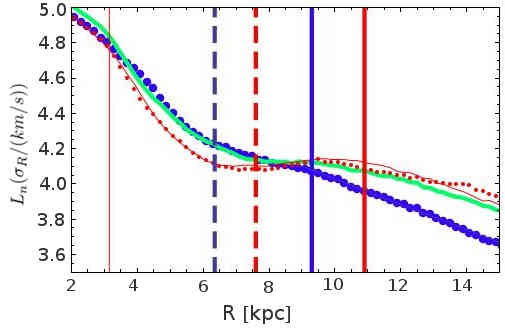
Figure 21: Profile of the radial velocity dispersion $\sigma_{R}(R)$ at four different times, namely $t=1.625$ Gyr (thick blue with points), $t=2$ Gyr (thick green solid), $t=2.5$ Gyr (dotted red) and $t=3$ Gyr (solid red). The dashed vertical lines mark the position of CR, and the solid vertical lines mark the position of the OLR at $t=1.625$ Gyr (blue) and $t=3$ Gyr (red) respectively.

Three more curves in Fig. 21, corresponding to $t=2,2.5$ and $3$ Gyr, show how the profile $\sigma_{R}$ versus $R$ evolves in time. At radii beyond the last position of the OLR ($R>11$ kpc), the velocity dispersion increases in time by a factor between $1.1$ and $1.2$ in a time interval $\sim 1.5$ Gyr, and the corresponding exponential profile becomes less steep. We notice, however, that the profile becomes nearly horizontal, leading to an ‘isothermalization’ (constant velocity dispersion) in a domain of the disc roughly between $R=6$ kpc and $R=11$ kpc. As seen in Fig. 21, the inner limit of this domain nearly coincides with the innermost position of CR (at $t=1.625$), while the outer limit nearly coincides with the outermost position of the OLR (at $t=3$ Gyr) in the considered time interval. One remarks that, as they move outward, at least one of these resonances visits part of the interval $6.5<R[kpc]<11$, in which the isothermalization takes place. Physically, the domain $R_{CR}<R<R_{OLR}$ is where chaotic motions completely dominate the dynamics. The corresponding particles belong to the well known ‘hot population’ (Sparke and Sellwood (1987)), whose orbits span the whole domain while recurrently entering also inside corotation. As a result, the strongly chaotic dynamics brings about an equalization of the velocity dispersion in the whole domain. On the other hand, we observe that the velocity dispersion profile remains practically invariant at distances smaller than the initial position of the ILR (at $\approx 3$ kpc). In fact, this resonance appears to act as a barrier for ‘heat’ (random kinetic energy) transfer across the disc.

The key remark, regarding the above evolution, is that although incidents of non-axisymmetric activity (in particular spirals) heat the outer parts of the disc, isothermalization in the domain scanned by the CR and OLR resonances implies that a part of the disc between CR and OLR becomes cooler with time. Physically, particles in the outer parts of the bar migrate outwards, carrying with them kinetic energy in the form of random motions. In Fig. 21, the initial and final profiles $\sigma_{R}(R)$ intersect at a radius $R_{c}\approx 8.5$ kpc. The bar’s co-rotation at the time of the initial profile is at $R_{CR}\approx 6.4$ kpc, while it shifts to $R^{\prime}_{CR}\approx 7.5$ kpc at the final time. Estimating by $R_{CR}<R<R_{c}$ the disc domain where manifolds rule the response of particles’ orbits to external perturbations, this domain has a width $\sim 2.1$ kpc at the initial time $t=1.6$ Gyr, which is limited to $\sim 1$ kpc at $t=3$ Gyr, while this domain is expected to shrink further to negligible widths as the bar’s co-rotation keeps moving outwards.

5 Discussion and conclusions

The origin and longevity of spiral structure in disc galaxies is still matter of intense debate. As new observational data and more accurate simulations come to surface, we gradually arrive at appreciating the potential complexity of the mechanisms which generate and maintain spiral structure. The co-existence and possible non-linear coupling of multiple patterns (see references in introduction) hints towards the chaotic nature of spiral arms, in particular when a strong bar is present. To the extent that spirals are bar driven, they are affected in a non-trivial way by the bar’s secular evolution. Within this context, the main contribution of the manifold theory is to describe what should be the expected form of the bar-driven spiral mode when the disc’s region between the bar’s Corotation and Outer Lindblad Resonance is largely chaotic. It should be stressed that the manifold theory poses no requirement that chaos originates exclusively from the bar. Nonlinear interaction of the bar mode with additional patterns beyond co-rotation actually enhances chaos (see references in text). Furthermore, it is a basic rule of dynamics that the unstable manifolds of one periodic orbit can intersect neither themselves nor the unstable manifolds of any other periodic orbit of equal Jacobi energy. Thus, all these manifolds have to ‘coalesce’ in nearly parallel directions, thus enhancing chaotic spirals.

The manifolds emanating from the region of the bar’s $L_{1}$ and $L_{2}$ points provide the simplest representation of these chaotic outflows. In the present paper we give evidence that these manifolds provide a dynamical skeleton in phase space, or, the dynamical avenues to be followed by new particles injected in the domain between CR and OLR at reccurent ‘incidents’ of non-axisymmetric activity. We gave a characterization of such incidents as of i) inner, or ii) outer origin, depending on whether the spectral analysis shows a wave originating inside CR and propagating outwards (in (i)), or originating outside CR, moving initially inwards, then being reflected at CR, and then moving outwards (in (ii)). Manifold spirals are connected with incidents of inner origin. Pattern detection algorithms such as Sobel-Feldman allow to detect the co-existence of various patterns, both at maxima and minima of the $m=2$ amplitude beyond the bar. We interpret the importance of manifolds as follows: whatever causes these incidents, at every incident the particles’ orbits (and in particular chaotic ones) are perturbed. Then, new particles injected in the CR zone tend to follow and populate the manifolds to a large extent, according to general rules of dynamics.

We argued that the continuous change of the form of the manifolds, as well as the motion, along the manifolds, of the matter which populates them, allows to reconcile manifold spirals with the multiplicity (and variability) of pattern speeds beyond the bar. A basic behavior is found to govern the evolution of the radial profile of the pattern frequency $\Omega_{2}(R)$ beyond the bar. At maxima of the non-axisymmetric activity $\Omega_{2}(R)$ tends to form a second plateau, indicating a second pattern speed outside CR, well distinct from $\Omega_{bar}$. At minima, the second plateau disappears, giving its place, to a shear-indicating decaying profile of the curve $\Omega_{2}(R)$. Remarkably, in the latter case, $\Omega_{2}(R)$ terminates at a value $\Omega_{2}\sim 0$ always near $R=R_{OLR}$. Five full cycles of this behavior are seen in our simulation, in a period of $\sim 1$ Gyr (see Fig. 20), leading to an approximate period of $\sim 0.2$ Gyr. This is in rough resonance with the bar’s period, but with large uncertainties in the numbers. On the other hand, since the comparison between manifolds and Sobel-Feldman-recognized patterns in the disc (Fig. 19) shows no appreciable differences between snapshots of minima and maxima of the non-axisymmetric activity, we argued that the degree to which manifolds are able to dictate the dynamics outside CR seems to be rather independent of the strength of any additional pattern in the disc.

In addition to well known mechanisms, we discussed a new mechanism which seems to play a key role in triggering new incidents of non-axisymmetric activity: this is the relative halo-disc orbit which results from the off-centering effect: whenever particles are ejected away from the disc through manifold spirals, the disc rebounces, leading to a relative orbit between the disc and the remaining spheroid (halo+bulge) component of the galaxy. We argue that even moderate off-centerings, of order $d/R_{d}\sim 0.1$, where $d$ is the off-center displacement and $R_{d}$ the disc’s exponential scale length, are able to induce appreciable $m=1$ tides on the disc (of order ${\cal O}(d/R_{d})$). The corelation between $d$ and the disc $m=1$ response is clearly seen in the disc’s spectral analysis. The way the $m=1$ tide affects the $m=2$ response beyond the bar appears to be a complex nonlinear phenomenon for which we have no precise analysis at present. Yet, the fact that one phenomenon influences the other is clearly seen in our simulation, as detailed in subsections 4.2 to 4.4.

As a final remark, we discussed the ‘thermal’ evolution of the disc, i.e., the way in which the radial profile of the velocity dispersion appears to be influenced in time due to non-axisymmetric activity. Owing, again, to the large degree of chaos between CR and OLR, we argued that the gradual outward shift of both the CR and OLR radii as the bar slows down, causes part of the disc, beyond the end of the bar, to acquire a nearly constant radial velocity dispersion. In fact, this ‘isothermalization’ causes a part of the disc, starting from inside the bar and ending at a point midway between CR and OLR to cool down. We interpret this effect as a hint that chaotic populations of particles gradually migrate outwards, carrying with them kinetic energy in the form of randomly oriented motions. Regarding, however, the responsiveness of the disc to manifold dynamics, we provide a heuristic argument showing that good levels of responsiveness should be limited in a domain which shrinks in time, as the CR radius moves outwards, while the radius beyond which the disc gets hotter in time is nearly fixed.

Appendix A Disc-halo relative displacement and $m=1$ perturbation on the disc

An estimate of the strength of the $m=1$ perturbation on the disc plane due to the disc-halo relative displacement can be obtained as follows: Consider a simplified model with two constituents, namely a razor-thin disc with exponential surface density profile $\Sigma(R)=\Sigma_{0}\exp(-R/R_{d})$, truncated at an inner radius $R_{1}$, and a spheroidal component (e.g. the combined halo-bulge system) represented by the spherical potential $V_{0}(r)$. Let O, the center of the disc, be the origin of the co-ordinates. We assume the center C of the spherical component to be displaced with respect to O, while remaining in the disc plane (as indicated by the simulations, see section 4). Let $\mathbf{d}$ be the displacement vector connecting O to C. Cartesian co-ordinates $(x,y)$ are defined such that the $x-$axis is parallel to $\mathbf{d}$.

The potential $V_{0}(r)$ expressed in polar co-ordinates $(R,\phi)$, with $x=R\cos\phi$, $y=R\sin\phi$, reads

$$\Phi(R,\phi)=V\left((R^{2}+d^{2}-2Rd\cos\phi\right)^{1/2})~{}~{},$$ (17)

where $d=|\mathbf{d}|$. For small displacements ($d<<R_{1}<R$), the potential (17) can be developed in powers of the ratio $d/R$. Up to first degree in $d/R$ we have:

$$\Phi(R,\phi)=V(R)-V^{\prime}(R)R\left({d\over R}\right)\cos\phi+{\cal O}\left(\left({d\over R}\right)^{2}\right)$$ (18)

As obvious from Eq. (18), the disc-halo relative displacement induces a $m=1$ component of the potential generated by the spherical component on the disc plane. Specifically, $\Phi(R,\phi)=\Phi_{0}(R)+\Phi_{1}(R)\cos\phi+...$, with

$$\Phi_{0}(R)=V(R),~{}~{}~{}\Phi_{1}(R)=-V^{\prime}(R)R\left({d\over R}\right)~{}~{}.$$ (19)

Higher order terms depending on the powers $(d/R)^{m}$, $m=2,3,\ldots$ are in general negligible. The residual $m=1$ gravitational field as measured by an observer constantly at the disc’s center of mass is found after subtracting a non-inertial term generated by the disc’s center-of-mass acceleration:

$$a_{d}=\left({d\over R_{d}}\right)\frac{\int_{R_{1}}^{\infty}\left(V^{\prime\prime}(R)R+V^{\prime}(R)\right)R_{d}e^{-R/R_{d}}dr}{\int_{R_{1}}^{\infty}e^{-R/R_{d}}rdr}$$ (20)

The residual potential is then given by

$$\Phi_{res}=\Phi_{d}(R)+\Phi_{0}(R)+\Phi_{1}(R)\cos\phi-a_{d}R\cos\phi+...$$ (21)

The importance of the term due to $a_{d}$ can be estimated for particular choices of potentials $V(R)$. For a Keplerian potential $V(R)\sim-GM/R$ we have

$$a_{d}\sim-c{GM\over R_{d}^{2}}\left({d\over R_{d}}\right),~{}~{}~{}c={1\over 2}\frac{\int_{R_{1}/R_{d}}^{\infty}e^{-\xi}\xi^{-2}d\xi}{\int_{R_{1}/R_{d}}^{\infty}e^{-\xi}\xi d\xi}$$ (22)

We find $c\sim 0.1$ for $R_{1}/R_{d}\sim 1$. Thus, $a_{d}$ is a factor $\sim 0.1(d/R_{d})$ smaller than the axisymmetric force produced by the spheroidal component on the disc at the distance $R\sim R_{d}$. We notice also that $a_{d}$ has a negative sign, i.e., as a result of their mutual displacement, the disc center of mass is repelled by the spheroidal component.

As an application, we will compute the relative amplitude of the $m=1$ component of the residual force in a potential $V(R)$ representing the sum of the bulge and halo components of our N-body simulation. The bulge is given by a Sersic law with scale length $r_{b}=1$ kpc, Sersic index $n=3.5$ and total mass $5\times 10^{9}M_{\odot}$. The halo is given by a double power-law density profile $\rho(r)=\rho_{0}(r/r_{h})^{-\alpha_{h}}(1+r/r_{h})^{\beta_{h}-\alpha_{h}}$ with $\alpha_{h}=1.3$, $\beta_{h}=3.5$, and $\rho_{0}=2.016\times 10^{8}$ $M_{\odot}/kpc^{3}$. We fit the total potential using a double Hernquist potential:

$$V_{fit}(R)=V_{0}-\sum_{i=1}^{2}{GM_{i}\over R+a_{i}}$$ (23)

with $V_{0}=2500Km^{2}/sec^{2}$, $a_{1}=0.5$ kpc, $a_{2}=3$ kpc, and $M_{1}=5\times 10^{9}M_{\odot}$, $M_{2}=6.2\times 10^{10}M_{\odot}$. The top panels in Fig. 22 show the fitting of the force produced by the spheroid by using the fitting formula (23) instead of the exact potential and forces of the adopted halo-bulge model. Finally, we consider an exponential disc with $R_{d}=3$ kpc, and $\Sigma_{0}=M_{d}/(2\pi R_{d}^{2})$, with $M_{d}=5\times 10^{10}M_{\odot}$. With the above formulas, the residual potential (21) is given by:

$$\Phi_{d}(R)=-G\Sigma_{0}\pi R\times~{}~{}~{}~{}~{}~{}~{}~{}~{}~{}~{}~{}~{}~{}~{}~{}~{}~{}~{}~{}~{}~{}~{}$$

$$\Bigg{(}I_{0}\left({R\over 2R_{d}}\right)K_{1}\left({R\over 2R_{d}}\right)-I_{1}\left({R\over 2R_{d}}\right)K_{0}\left({R\over 2R_{d}}\right)\Bigg{)}$$ (24)

$$\Phi_{0}(R)=-\sum_{i=1}^{2}{GM_{i}\over R+a_{i}},~{}~{}~{}\Phi_{1}(R)=-\sum_{i=1}^{2}{GM_{i}d\over(R+a_{i})^{2}}$$ (25)

$$a_{d}=-\sum_{i=1}^{2}c_{i}{GM_{i}d\over R_{d}^{3}},~{}c_{i}={1\over 2}\frac{\int_{\xi_{1}}^{\infty}e^{-\xi}\left({\xi-a^{\prime}_{i}\over\xi(\xi+a^{\prime}_{i})^{3}}\right)d\xi}{\int_{\xi_{1}}^{\infty}e^{-\xi}\xi d\xi}~{}~{}.$$ (26)

$I_{0},I_{1},K_{0},K_{1}$ are cylindrical Bessel functions, and $a^{\prime}i=a_{i}/R_{d}$, $\xi_{1}=R_{1}/R_{d}$. Differentiating the potential (21) obtained through the above formulas, we find the residual forces $F_{R,res}=-\partial\Phi_{res}/\partial R$, $F_{\phi,res}=-(1/R)\partial\Phi_{res}/\partial\phi$ as:

$$F_{R,res}(R,\phi) = f_{0}(R)+f_{1}(R)\cos\phi,~{}~{}~{}$$ (27)

$$F_{\phi,res}(R,\phi) = g_{1}(R)\sin\phi~{}~{}.$$

Figure 22 shows the absolute ratio $|(f_{1}^{2}+g_{1}^{2})^{1/2}/f_{0}|$ for the adopted model parameters, as a function of the distance $R$ from the disc center, for three values of the displacement $d=0.05,0.15$ and $0.25$ kpc. One notices that even small displacements result in $m=1$ fields of amplitude a few percent in the inner parts of the disc. In particular, for the largest observed displacement in the simulation, $d=0.25$ kpc, the $m=1$ relative amplitude exceeds $5\%$ at the disc’s inner $3$ kpc, and $10\%$ inside the inner $2$ kpc.

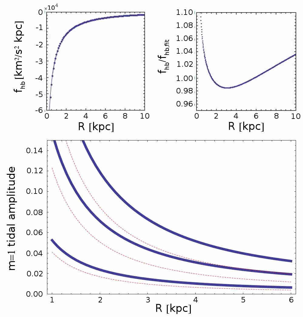
Figure 22: Top left: comparison between the halo-bulge combined central force per unit mass $f_{hb}$ as a function of the radius $R$ and the force $f_{hb,fit}$ from the double-Hernquist fitting formula (Eq:23) with the adopted parameters (see text). Top right: the ratio $f_{hb}/f_{hb,fit}$ as a function of $R$. Bottom: the absolute ratio $|(f_{1}^{2}+g_{1}^{2})^{1/2}/f_{0}|$ of the $m=1$ over axisymmetric force when the halo-bulge displacement is $d=0.25$ kpc,$d=0.15$ kpc or $d=0.05$ kpc (top, middle and bottom pairs of curves respectively). The solid blue curves correspond to $f_{0}$ being computed using the halo-bulge pair only, while for the red dashed curves $f_{0}$ includes also the disc axisymmetric force.

References

- Antoja et al. (2014) Antoja, T, Helmi, A., Dehnen, W., et al.: 2014, A&A, 563, 60
- Athanassoula (2002) Athanassoula, E.: 2002, ApJ, 569, L83
- Athanassoula (2003) Athanassoula, E.: 2003, MNRAS, 341, 1179
- Athanassoula (2007) Athanassoula, E.: 2007, MNRAS, 377, 1569
- Athanassoula & Misiriotis (2002) Athanassoula, E., and Misiriotis, A.: 2002, MNRAS, 330, 35
- Athanassoula et al. (2009a) Athanassoula, E., Romero-Gómez, M., Masdemont, J. J.: 2009a, MNRAS, 394, 67
- Athanassoula et al. (2009b) Athanassoula, E., Romero-Gómez, M., Bosma, A., Masdemont, J.J.: 2009b, MNRAS, 400, 1706
- Athanassoula et al. (2010) Athanassoula, E., Romero-Gómez, M., Bosma, A., Masdemont, J.J.: 2010, MNRAS, 407, 1433
- Athanassoula (2012) Athanassoula, E.: 2012, MNRAS, 426, L46
- Athanassoula (2013) Athanassoula, E.: 2013, in ‘Secular Evolution of Galaxies’, XXIII Canary Islands Winter School of Astrophysics. J Falcon-Barroso and J. H. Knapen (eds), Cambridge University Press, pp.305-352.
- Avila-Reese et al. (2005) Avila-Reese, V., Carrillo, A., Valenzuela, O., and Klypin, A.: 2005, MNRAS, 361, 997
- Baba et al. (2013) Baba, J., Saitoh, T.R., Wada, K.: 2013, ApJ, 763, 46
- Baba (2015) Baba, J.: 2015, MNRAS, 454, 2954
- Berentzen et al. (2006) Berentzen, I., Shlosman, I., and Jogee, S.: 2006: ApJ, 637, 582
- Binney & Tremaine (2008) Binney J., and Tremaine S.: 2008, Galactic Dynamics, second edn. Princeton University Press
- Binney (2013) Binney, J.: 2013, in ‘Secular Evolution of Galaxies’, XXIII Canary Islands Winter School of Astrophysics. J Falcon-Barroso and J. H. Knapen (eds), Cambridge University Press, pp.259-304.
- Bland-Hawthorn & Gerhard (2016) Bland-Hawthorn, J., and Gerhard, O.: 2016, Annu. Rev. A&A Astrophys., 54, 529
- Boonyasait et al. (2005) Boonyasait, V., Patsis, P.A., and Gottesman, S.T: 2005, NYASA, 1045, 203
- Bureau & Athanassoula (1999) Bureau, M., and Athanassoula, E.: 1999, ApJ, 522, 686
- Bureau & Athanassoula (2005) Bureau, M., and Athanassoula, E. 2005, ApJ, 626, 159
- Chirikov (1979) Chirikov, B.V.: 1979, Phys. Rep., 52, 263
- Combes & Sanders (1981) Combes, F., and Sanders, R.H.: 1981, A&A, 96, 164
- Combes et al. (1990) Combes, F., Debbasch, F., Friedli, D., and Pfenniger, D.: 1990, A&A, 233, 82
- Contopoulos (1980) Contopoulos,G.: 1980, A&A, 81, 198
- Contopoulos (2002) Contopoulos,G.: 2002, ‘Order and Chaos in Dynamical Astronomy’, Springer
- Danby (1965) Danby, J.M.A., 1965: AJ, 70, 501
- Debattista & Sellwood (1998) Debattista, V.P., and Sellwood, J.A.: 1998, ApJ, 493, L5
- Debattista & Sellwood (2000) Debattista, V.P., and Sellwood, J.A.: 2000, ApJ, 543, 704
- Debattista et al. (2006) Debattista, V. P., Mayer, L., Carollo, C. M., Moore, B., Wadsley, J., and Quinn, T.: 2006, ApJ, 645, 209
- Debattista (2006) Debattista, V.P.: 2006, ASPC, 352, 161
- Dobbs and Baba (2014) Dobbs, C. and Baba, J.: 2014, Pub. Astron. Soc. Australia, 31, 40.
- Dubinski et al. (2009) Dubinski, J., Berentzen, I., and Shlosman, I.: 2009, ApJ 697, 293
- Efthymiopoulos (2010) Efthymiopoulos, C., 2010: Eur. Phys. J. Special Topics, 186, 91
- Falcon-Barroso and Knapen (2013) Falcon-Barroso, J. and Knapen, J.H.: 2013, ‘Secular Evolution of Galaxies’, XXIII Canary Islands Winter School of Astrophysics. Cambridge University Press
- Font et al. (2014) Font, J., Beckman, J.E., Querejeta, M., Epinat, B., James, P.A., Blasco-herrera, J., Erroz-Ferrer, S., Pérez, I.: 2014, ApJS, 210, 2
- Gonzalez & Woods (1992) Gonzalez, R., and Woods, R.: 1992, ‘Digital Image Processing’, Addison Wesley
- Grobman (1959) Grobman, D.M.: 1959, Dokl. Akad. Nauk SSSR 128, 880
- Hamilton et al. (2018) Hamilton, C., Fouvry, J.B., Binney, J., and Pichon, C.: 2018, MNRAS, tmp.2180
- Harsoula et al. (2016) Harsoula, M., Efthymiopoulos, C., and Contopoulos, G.: 2016, MNRAS, 459, 3419
- Hartman (1960) Hartman, P.: 1960, Proc. Amer. Math. Soc. 11, 610
- Hohl (1971) Hohl, F.: 1971, ApJ, 168, 343
- Holley-Bockelmann et al. (2005) Holley-Bockelmann, K., Weinberg, M., and Katz, N.: 2005, MNRAS, 363, 991
- Junqueira et al. (2015) Junqueira, T.C., Chiappini, C., L epine, J.R.D., Minchev, I., Santiago, B.X.: 2015, MNRAS 449, 2336
- Kalapotharakos et al. (2010) Kalapotharakos, C., Patsis, P.A., Grosbøl, P: 2010, MNRAS, 403, 83
- Kormendy & Kennicutt (2004) Kormendy, J., and Kennicutt, R.C.: 2004, ARA&A, 42, 603
- Kormendy (2013) Kormendy, J.: 2013, in ‘Secular Evolution of Galaxies’, XXIII Canary Islands Winter School of Astrophysics. J Falcon-Barroso and J. H. Knapen (eds), Cambridge University Press, pp.1-154.
- Kwak et al. (2017) Kwak, S., Kim, W.T, Rey, S.C, Kim, S.: 2017, ApJ, 839, 24
- Kyziropoulos et al. (2016) Kyziropoulos, P., Efthymiopoulos, C., Gravannis, G., and Patsis, P.: 2016, MNRAS, 463, 2210
- Kyziropoulos et al. (2017a) Kyziropoulos, P., Filelis-Papadopoulos, C.K., Gravvanis, G., and Efthymiopoulos, C.: 2017. ‘A parallel Self Mesh-Adaptive N-body method based on approximate inverses’. J. Supercomputing, Online first, DOI 10.1007/s11227-017-2078-7
- Kyziropoulos et al. (2017b) Kyziropoulos, P., Filelis-Papadopoulos, C.K., Gravvanis, G., and Efthymiopoulos, C.: 2017, ‘Toward the design of a novel hybrid parallel N-body method in scope of modern cloud architectures’, J. Supercomputing, online first, DOI 10.1007/s11227-017-2140-5
- Little & Carlberg (1991) Little, B., and Carlberg, R.G.: 1991, MNRAS, 250, 161
- Lokas (2016) Lokas, E: 2016, ApJ, 830, 20L
- Lynden-Bell & Kalnajs (1972) Lynden-Bell, D., and Kalnajs, A.J.: 1972, MNRAS, 157, 1
- Martinez-Valpuesta & Shlosman (2004) Martinez-Valpuesta, I., and Shlosman, I.: 2004, ApJ, 613, 29
- Martinez-Valpuesta et al. (2006) Martinez-Valpuesta, I., Shlosman, I., and Heller, C.: 2006, ApJ, 637, 214
- Masset & Tagger (1997) Masset, F., Tagger, M.: 1997, A&A, 322, 442
- McMillan & Dehnen (2005) McMillan, P.J., and Dehnen, W.: 2005, MNRAS, 363, 1205
- Meidt et al. (2009) Meidt, S.E., Rand, R.J., and Merrifield, M.R.: 2009, ApJ, 702, 277
- Minchev & Quillen (2006) Minchev, I., and Quillen, A.C.: 2006, MNRAS, 368, 623
- Minchev et al. (2012) Minchev, I., Famaey, B., Quillen, A.C., Di Matteo, P., Combes, F., Vlajić, M., Erwin, P., Bland-Hawthorn, J.: 2012, A&A, 548, 126
- OŃeill & Dubinski (2003) O’Neill, J.K., and Dubinski, J.: 2003, MNRAS, 346, 251
- Patsis et al. (1997) Patsis, P.A., Efthymiopoulos, C., Contopoulos, G., and Voglis, N.: 1997, A&A, 326, 493
- Patsis (2006) Patsis, P.: 2006, MNRAS, 369, L56
- Patsis et al. (2009) Patsis, P.A., Kaufmann, D.E., Gottesman, S.T.and Boonyasait, V.: 2009, MNRAS, 394, 142
- Pérez-Villegas et al. (2015) Pérez-Villegas, A., Pichardo, B. and Moreno, E.: 2015, ApJ, 809, 170
- Pfenniger & Friedli (1991) Pfenniger, D., and Friedli, D.: 1991, A&A, 252, 75
- Quillen (2003) Quillen, A.C.: 2003, ApJ, 125, 785
- Quillen et al. (2011) Quillen, A.C., Dougherty, J., Bagley, M.B., Minchev, I., Comparetta, J.: 2011, MNRAS, 417, 762
- Raha et al. (1991) Raha, N., Sellwood, J.A., James, R.A., and Kahn, F.D.: 1991, Nat, 352, 411
- Rautiainen & Salo (1999) Rautiainen, P., Salo, H.: 1999, A&A, 348, 737
- Roca-Fabrega et al. (2013) Roca-Fàbrega, S, Valenzuela, O., Figueras, F., Romero-Gómez, M., Vel’azquez, H., Antoja, T., Pichardo, B: 2013, MNRAS, 432, 2878
- Romero-Gomez et al. (2006) Romero-Gomez, M., Masdemont, J.J., Athanassoula, E. and Garcia-Gomez, C.: 2006, A&A, 453, 39
- Romero-Gomez et al. (2007) Romero-Gomez, M., Athanassoula, E., Masdemont, J.J. and Garcia-Gomez, C.: 2007, A&A, 472, 63
- Sellwood & Sparke (1988) Sellwood, J.A., and Sparke, L.S.: 1988, MNRAS, 231, 25
- Sellwood & Wilkinson (1993) Sellwood, J.A., Wilkinson, A.: 1993, RPPh, 56, 173
- Sellwood & Binney (2002) Sellwood, J.A., and Binney, J.J.: 2002, MNRAS, 336, 785
- Sellwood (2003) Sellwood, J. A. 2003, ApJ, 587, 638
- Sellwood (2014) Sellwood, J.A.: 2014, RvMP, 86, 1
- Sparke and Sellwood (1987) Sparke, L. S. and Sellwood, J. A., 1987, MNRAS, 225, 653
- Speights and Westpfahl (2012) Speights, J.C., and Westpfahl, D.J.: 2012, ApJ, 752, 52
- Speights & Rooke (2016) Speights, J.C., and Rooke, P.: 2016, ApJ, 826, 2
- Struck (2015) Struck, C.: 2015, MNRAS, 450, 2217
- Tagger et al. (1987) Tagger, M., Sygnet, J.F., Athanassoula, E., Pellat,R.: 1987, ApJ, 318, 43.
- Tagger & Athanassoula (1991) Tagger, M.; Athanassoula, E.: 1991, IAUS, 146, 105
- Toomre and Kalnajs (1991) Toomre, A., and Kalnajs, A.J.: 1991, in B. Sundelius (ed), ‘Dyamics of Disc Galaxies’, Göteborgs University, p. 341.
- Tremaine & Weinberg (1984) Tremaine, S., and Weinberg, M.D.: 1984, ApJ, 282, L5
- Tsoutsis et al. (2008) Tsoutsis, P., Efthymiopoulos, C. and Voglis, N.: 2008, MNRAS, 387, 1264
- Tsoutsis et al. (2009) Tsoutsis, P., Kalapotharakos, C., Efthymiopoulos, C. and Contopoulos, G.: 2009, A&A, 495, 743
- Vera-Villamizar et al. (2001) Vera-Villamizar, N., Dottori, H., Puerari, I., and de Carvalho, R.: 2001, ApJ, 547, 187
- Voglis et al. (2006a) Voglis, N., Tsoutsis, P. and Efthymiopoulos, C.: 2006a, MNRAS, 373, 280
- Voglis et al. (2006b) Voglis, N., Stavropoulos, I. and Kalapotharakos, C.: 2006b, MNRAS, 372, 901
- Weinberg & Katz (2007) Weinberg, M.D., and Katz, N.: 2007, MNRAS, 375, 460
- Wiggins (1990) Wiggins, S.: 1990, ‘Introduction to Nonlinear Dynamical Systems and Chaos’, Springer, New York
- Wu et al. (2016) Wu, Y-T, Pfenniger, D., and Taam, R.E.: 2016, ApJ, 830, 111