Complexity and Near Extremal Charged Black Branes

Mohsen Alishahiha^∗, Komeil Babaei Velni^† and Mohammad Reza Tanhayi^‡,∗

^∗ School of Physics, Institute for Research in Fundamental Sciences (IPM)
P.O. Box 19395-5531, Tehran, Iran
^† Department of Physics, University of Guilan, P.O. Box 41335-1914, Rasht, Iran
^‡ Department of physics, Islamic Azad University Central Tehran Branch, Tehran, Iran

E-mails: alishah@ipm.ir, babaeivelni@guilan.ac.ir, mtanhayi@ipm.ir

We compute holographic complexity of charged black brane solutions in arbitrary dimensions for the near horizon limit of near extremal case using two different methods. The corresponding complexity may be obtained either by taking the limit from the complexity of the charged black brane, or by computing the complexity for near horizon limit of near extremal solution. One observes that these results coincide if one assumes to have a cutoff behind horizon whose value is fixed by UV cutoff and also taking into account a proper counterterm evaluated on this cutoff. We also consider the situation for Vaidya charged black branes too.

1 Introduction

In the context of black hole physics, horizon, black hole entropy, information paradox and physics behind the horizon are in the center of the most studies in last several decades. Quantum information theory might be capable to shed light on these subjects. Indeed, recent progress on black hole physics has opened up a possibility to make a connection between quantum information theory and back hole physics (see [1] and its citations). To explore and understand this possible connection the AdS/CFT correspondence [2] has played rather an important role. In this context holographic entanglement entropy [3] and computational complexity[4, 5] may be thought of as examples which could make this connection more concrete.

In particular, holographic complexity, by definition, might be able to give us some information on the physics behind the horizon. To elaborate this point better it is worth noting that the holographic complexity may be obtained by the on shell action evaluated on a certain subregion of spacetime known as the Wheeler-DeWitt (WDW) patch[6, 7], that includes some portion of the spacetime located behind the horizon.

More precisely, in this picture known as “complexity equals to action” (CA) proposal [6, 7] the late time behavior of complexity growth is entirely given by the on shell action evaluated on the intersection of the WDW patch with the future interior[8], leading to an observation that the late time behavior of holographic complexity is insensitive to the UV cutoff [9]. This, in turn, results in a conclusion that there could be a relation between the UV cutoff and a cutoff that should be defined behind the horizon [9, 10] whose the value is fixed by the UV cutoff. Indeed this is an interesting feature of complexity that could probe physics behind the horizon.

It is important to mention that the result of [9] leading to the behind the horizon cutoff relies on two facts. The first one is what we just mentioned, namely, the late time behavior of complexity is UV blind. The second one is that, according to Lloyd’s bound [11], the late time behavior of the complexity growth is given in terms of the energy of the system that is sensitive to the finite UV cutoff.

We note, however, that in the context of holographic complexity it is known that the Lloyd’s bound may be violated [12, 13, 14, 15, 16, 17]. Nonetheless, the violation of Lloyd’s bound just modifies the relation between the cutoff behind the horizon and the UV cutoff and the Lloyd’s bound violation does not affect the main conclusion. Indeed, the only fact we need is that the late time behavior of complexity growth is controlled by physical charges defined at the boundary of which the values are affected by a finite UV cutoff.

This is the aim of the present paper to further explore the significance of the cutoff behind the horizon. To do so, we will study holographic complexity for AdS-Reissner-Nordström (AdS-RN) black branes in arbitrary dimensions (see also [18, 12, 19, 20]). More precisely, we will consider near horizon limit of near extremal charged black branes and compute complexity in two different ways. In the first approach we will obtain the corresponding rate of complexity growth by taking the near extremal limit of the complexity growth of the charged black brane. In the second approach we compute complexity for a metric obtained by taking near horizon limit of the near extremal AdS-RN black brane that has the form of AdS${}_{2}\times\mathbb{R}^{d-1}$.

It is important to note that if one naively computes complexity for geometries containing an AdS₂ factor the late time growth vanishes [9, 21, 22] that is not consistent with what we may get from taking near extremal limit of the complexity growth. On the other hand, as we will see, following [9] if one considers the cutoff behind the horizon whose value is fixed by the UV cutoff, then one finds the standard late time linear growth that is exactly the one obtained by the first approach. It is, however, important to note that in order to get a consistent result one needs also to consider all counter terms already obtained in the context of holographic renormalization [10].

Indeed, we believe that the result of the present paper should be considered as an evidence supporting the proposed idea that the UV cutoff will automatically fix a cutoff behind the horizon. Moreover, it also explores the role of the counter terms which are required by holographic renormalization.

The organization of the paper is as follows. In the next section in order to fix our notations we will review the computation of complexity for charged black branes. In section three we will study near horizon limit of near extremal cases where we compute the corresponding complexity from two different approaches. In section four we will redo the same computations for charged Vaidya black brane. The last section is devoted to summery and conclusions.

2 Complexity of charged black branes: a brief review

In this section in order to fix our notation we will review holographic complexity for charged black branes using CA proposal. Actually the full time dependence of the complexity growth for charged black holes has been first studied in [12]. The aim of this section is, while reviewing the CA proposal for charged black branes, presenting a closed inspiring form for the corresponding holographic complexity. To do so, we will use an appropriate coordinate system that simplifies the computations rather significantly. Although the result is known the presentation is new and by itself is interesting.

To proceed, let us consider an Einstein-Maxwell theory in $d+1$ dimensions of which the action may be given as follows

$$I_{0}=\frac{1}{16\pi G_{N}}\int d^{d+1}x\sqrt{-g}\left(R+\frac{d(d-1)}{L^{2}}-\frac{1}{2}F_{\mu\nu}F^{\mu\nu}\right)\,,$$ (2.1)

where $G_{N}$ is the Newton’s constant and $L$ is a length scale in the theory. The corresponding equations of motion are

$$R_{\mu\nu}-F_{\alpha\mu}F^{\alpha}_{\,\nu}-\frac{1}{2}\left(R+\frac{d(d-1)}{L^{2}}-\frac{1}{2}F^{2}\right)g_{\mu\nu}=0,\;\;\;\;\;\;\;\partial_{\alpha}\left(\sqrt{-g}F^{\alpha\beta}\right)=0\,.$$ (2.2)

These equations admit AdS-RN black brane solutions that for $d\geq 3$ are given by

$$ds^{2}=\frac{L^{2}}{r^{2}}\left(-f(r)dt^{2}+\frac{dr^{2}}{f(r)}+\sum_{i=1}^{d-1}d{x}_{i}^{2}\right),\;\;\;\;\;f(r)=1-mr^{d}+{Q^{2}}r^{2(d-1)},$$ (2.3)

(2.4)

$$A_{t}=\sqrt{\frac{d-1}{d-2}}QL\;(r_{+}^{d-2}-r^{d-2}),$$ (2.5)

where $m$ and $Q$ are related to the mass and charge of the black brane solution, respectively. Moreover, $r_{+}$ is the radius of horizon that is the smallest solution of $f(r)=0$ ( note that in our notation the boundary is at $r=0$). For $d=2$ the solution exhibits a logarithmic behavior.

Now, the aim is to compute holographic complexity for the above charged black brane using CA proposal. To do so, one needs to compute on shell action on the WDW patch associated with a boundary state given at $\tau=t_{L}+t_{R}$. Here $t_{L}(t_{R})$, is time coordinate of left (right) boundary of the charged black brane (see left panel of the figure 1). To proceed, we note that the action consists of several parts including bulk, boundary and joint points as follows [23, 24, 25]

$$I = I_{0}+\frac{1}{8\pi G_{N}}\int_{\Sigma^{d}_{t}}K_{t}\;d\Sigma_{t}\pm\frac{1}{8\pi G_{N}}\int_{\Sigma^{d}_{s}}K_{s}\;d\Sigma_{s}\pm\frac{1}{8\pi G_{N}}\int_{\Sigma^{d}_{n}}K_{n}\;dSd\lambda$$ (2.8)

$$\pm\frac{1}{8\pi G_{N}}\int_{J^{d-1}}a\;dS\pm\frac{1}{8\pi G_{N}}\int_{\Sigma^{d}_{n}}d\lambda dS\,\Theta\log\frac{|L\Theta|}{d-1}\,.$$

Here the timelike, spacelike, and null boundaries and also joint points are denoted by $\Sigma_{t}^{d},\Sigma_{s}^{d},\Sigma_{n}^{d}$ and $J^{d-1}$, respectively. The extrinsic curvature of the corresponding boundaries are given by $K_{t},K_{s}$ and $K_{n}$. The function $a$ at the intersection of the boundaries is given by the logarithm of the inner product of the corresponding normal vectors and $\lambda$ is the null coordinate defined on the null segments. The sign of different terms depends on the relative position of the boundaries and the bulk region of interest (see [25] for more details). Moreover, in the last term the quantity $\Theta$ is defined as follows

$$\Theta=\frac{1}{\sqrt{\gamma}}\frac{\partial\sqrt{\gamma}}{\partial\lambda},$$ (2.9)

where $\gamma$ is determinant of induced metric on the joint points. This term is needed in order to remove the ambiguity associated with the normalization of null vectors [25, 26]. As we will see this term together with other counterterms play crucial role in order to get desired results.

It is worth noting that in general to write the last term one could use an arbitrary length scale, though for simplicity we have fixed the corresponding scale to be the radius of curvature $L$. This choice just removes the most divergent term from the complexity and does not affect the physics that we are interested in.

It is also important to note that besides the above terms, there are also other boundary terms which could contribute to the complexity. These terms are those counterterms needed to make the on shell action finite when evaluated over whole spacetime[27]. The importance of these terms have been also known from holographic renormalization point of view (see e.g.[28]). In the present case since the solution has flat boundary the only term remains to be considered is (for asymptotically AdS_d+1 metric)

$$I^{\rm c.t.}=\frac{1}{8\pi G_{N}}\int d\Sigma\,\,\frac{d-1}{L}\,.$$ (2.10)

Note that this term gives non-zero contributions to the holographic complexity whenever the corresponding WDW patch contains space like or time like boundaries. More precisely, for a time like boundary at the UV region of the space time, typically, this counter term needed to remove certain divergent term. Of course it may also have a finite contribution to the complexity as well, though its contribution does not change the complexity growth. On the other hand, for a space like boundary (that typically appears behind the horizon) this term might lead to a time dependent contribution to the complexity. This is, indeed, the point we are going to explore in the next section.

It is obvious that for the charged black brane (2.3) and the corresponding WDW patch shown in the left panel of the figure 1, since all boundaries are null, this term vanishes identically, though as we will see for the case in which the WDW patch contains a space like boundary this term gives a non-zero contribution to the on shell action (see eq. (3.13)).

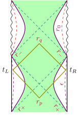
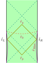
Figure 1: Left : Penrose diagram of a charged black brane and the WDW patch associated with the sate defined at $\tau=t_{R}+t_{L}$. The green region shows the Penrose diagram of near extremal limit of the charged black brane. The red dashed lines is a timelike cutoff behaind the horizon. Right: Penrose diagram of an AdS₂ geometry which can be thought of as near horizon limit of the near extremal solution. The corresponding WDW patch is cut by the behind the horizon cutoff $\hat{r}_{0}$ that is fixed by the UV cutoff $\hat{r}_{\rm Max}$.

Let us now compute on shell action for the WDW patch depicted in the left panel of the figure 1. To do so, it is found useful to consider the following change of coordinate

$$dt=dv+\frac{dr}{f(r)}\,,$$ (2.11)

by which the solution (2.3) may be recast into the following form

$$ds^{2}=\frac{L^{2}}{r^{2}}\left(-f(r)dv^{2}-2drdv+d\vec{x}^{2}\right),\;\;\;\;\;\;A_{v}=\sqrt{\frac{d-1}{d-2}}QL\;(r_{+}^{d-2}-r^{d-2})$$ (2.12)

In this notation the null boundaries of the corresponding WDW patch are given by $v=$constant and $u=$constant. Here, the coordinate $u$ defined by $du=dt+\frac{dr}{f(r)}$. Of course since we are using $(r,v)$ coordinate system one needs to write $u$ coordinate in terms of $r$ and $v$

$$du=dv+2\frac{dr}{f(r)}.$$ (2.13)

Therefore the null boundaries are given by $v=-t_{L}$ and $v=t_{R}$ for constant $v$ and, for constant $u$ one ends up with following equations for boundaries

$$\int_{-t_{L}}^{v}dv=-2\int_{\epsilon}^{r_{q}(v,\tau)}\frac{dr}{f(r)}\,\,\,\,\rightarrow\,\,\,v+t_{L}=-2\int_{\epsilon}^{r_{q}(v,\tau)}\frac{dr}{f(r)},$$ (2.14)

(2.15)

$$\int_{t_{R}}^{v}dv=-2\int_{\epsilon}^{r_{p}(v,\tau)}\frac{dr}{f(r)}\,\,\,\,\rightarrow\,\,\,t_{R}-v=2\int_{\epsilon}^{r_{p}(v,\tau)}\frac{dr}{f(r)}.$$ (2.16)

Before proceeding to compute the on shell action it is useful to fix our notation for the null vectors of the null boundaries of the corresponding WDW patch. Indeed, as we have already mentioned the boundaries are given at $u$ and $v$ constant. Therefore the corresponding null vectors are given by

$$k_{1}=\alpha\partial_{v},\;\;\;\;\;\;\;\;\;k_{2}=\beta\partial_{u}=\beta\left(\partial_{v}+\frac{2}{f(r)}\partial_{r}\right),$$ (2.17)

where $\alpha$ and $\beta$ are two free parameters appearing due to the ambiguity of the normalization of null vectors.

For the charged black brane which we are considering one has

$$\sqrt{-g}\left(R+\frac{d(d-1)}{L^{2}}-\frac{1}{2}F^{2}\right)=-2d\frac{L^{d-1}}{r^{d+1}}+2(d-2)L^{d-1}Q^{2}r^{d-3}\,,$$ (2.18)

by which the bulk part of the on shell action reads

$$I^{\rm bulk} = \frac{L^{d-1}}{8\pi G_{N}}\int d^{d-1}x\;\int_{-t_{L}}^{t_{R}}dv\int_{r_{p}(v,\tau)}^{r_{q}(v,\tau)}dr\,\left(\frac{-d}{r^{d+1}}+Q^{2}(d-2)r^{d-3}\right)$$ (2.19)

$$= \frac{V_{d-1}L^{d-1}}{8\pi G_{N}}\int_{-t_{L}}^{t_{R}}dv\left(\frac{f(r_{q}(v,\tau))}{r_{q}^{d}(v,\tau)}-\frac{f(r_{p}(v,\tau))}{r_{p}^{d}(v,\tau)}\right).$$ (2.21)

On the other had using the fact that $\frac{dr_{p}(v,\tau)}{d\tau}=\frac{1}{2}f(r_{p}(v,\tau))$ and $\frac{dr_{q}(v,\tau)}{d\tau}=-\frac{1}{2}f(r_{q}(v,\tau))$ one can perform the above integration resulting in

$$I^{\rm bulk}=\frac{V_{d-1}L^{d-1}}{8\pi G_{N}}\left(\frac{2}{(d-1)r_{p}^{d-1}(\tau)}+\frac{2}{(d-1)r_{q}^{d-1}(\tau)}-\frac{4}{(d-1)\epsilon^{d-1}}\right)\,.$$ (2.22)

Here we have used the fact that in our notation one has $r_{p}(\tau)=r_{p}(-t_{L},\tau),r_{q}(\tau)=r_{q}(t_{R},\tau)$ and $r_{p}(t_{R},\tau)=r_{q}(-t_{L},\tau)=\epsilon$.

Since all boundaries are null their contributions vanish using Affine parameterization for null direction, while for the joint points using (2.17) one gets

$$I^{\rm joint} = \frac{V_{d-1}L^{d-1}}{8\pi G_{N}}\left(\frac{\log\frac{\alpha\beta r^{2}_{p}(\tau)}{L^{2}|f(r_{p})|}}{r_{p}^{d-1}(\tau)}+\frac{\log\frac{\alpha\beta r^{2}_{q}(\tau)}{L^{2}|f(r_{q})|}}{r_{q}^{d-1}(\tau)}-2\frac{\log\frac{\alpha\beta\epsilon^{2}}{L^{2}f(\epsilon)}}{\epsilon^{d-1}}\right)$$ (2.23)

$$= \frac{V_{d-1}L^{d-1}}{8\pi G_{N}}\left(\frac{\log\frac{\alpha\beta r^{2}_{p}(\tau)}{L^{2}}}{r_{p}^{d-1}(\tau)}+\frac{\log\frac{\alpha\beta r^{2}_{q}(\tau)}{L^{2}}}{r_{q}^{d-1}(\tau)}-2\frac{\log\frac{\alpha\beta\epsilon^{2}}{L^{2}}}{\epsilon^{d-1}}-\frac{\log{|f(r_{p})|}}{r_{p}^{d-1}(\tau)}-\frac{\log{|f(r_{q})|}}{r_{q}^{d-1}(\tau)}\right).$$ (2.25)

The last contribution to the on shell action we need to consider is the contribution of the term required to remove the ambiguity associated with the normalization of null vectors. There are indeed four null boundaries whose contributions to the on shell action are

$$I^{\rm amb} = \frac{V_{d-1}L^{d-1}}{8\pi G_{N}}\left(-\frac{\log\frac{\alpha\beta r^{2}_{p}(\tau)}{L^{2}}}{r_{p}^{d-1}(\tau)}-\frac{2}{(d-1)r_{p}^{d-1}(\tau)}+\frac{\log\frac{\alpha\beta\epsilon^{2}}{L^{2}}}{\epsilon^{d-1}}+\frac{2}{(d-1)\epsilon^{d-1}}\right)$$ (2.28)

$$+\frac{V_{d-1}L^{d-1}}{8\pi G_{N}}\left(-\frac{\log\frac{\alpha\beta r^{2}_{q}(\tau)}{L^{2}}}{r_{q}^{d-1}(\tau)}-\frac{2}{(d-1)r_{q}^{d-1}(\tau)}+\frac{\log\frac{\alpha\beta\epsilon^{2}}{L^{2}}}{\epsilon^{d-1}}+\frac{2}{(d-1)\epsilon^{d-1}}\right)\,.$$

Now putting all terms together one finds the following expression for the total on shell action evaluated in the WDW patch

$$I^{\rm total}=-\frac{V_{d-1}L^{d-1}}{8\pi G_{N}}\left(\frac{\log{|f(r_{p}(\tau))|}}{r_{p}^{d-1}(\tau)}+\frac{\log{|f(r_{q}(\tau))|}}{r_{q}^{d-1}(\tau)}\right)\,.$$ (2.29)

Interestingly enough, the final result is very simple and indeed consists of the contributions of two joint points $p$ and $q$. It is also easy to compute its time derivative to find

$$\frac{dI^{\rm total}}{d\tau} = \frac{V_{d-1}L^{d-1}}{16\pi G_{N}}\bigg{(}\frac{{f^{\prime}(r_{q}(\tau))}}{r_{q}^{d-1}(\tau)}-\frac{{f^{\prime}(r_{p}(\tau))}}{r_{p}^{d-1}(\tau)}$$

$$\;\;\;\;\;\;\;\;\;\;\;\;\;\;\;\;\;\;+\frac{(d-1)}{r_{p}^{d}(\tau)}f(r_{p}(\tau))\log{|f(r_{p}(\tau))|}-\frac{(d-1)}{r_{q}^{d}(\tau)}f(r_{q}(\tau))\log{|f(r_{q}(\tau))|}\bigg{)},$$

which at the late time reads

$$\frac{dI^{\rm total}}{d{\tau}}=\frac{V_{d-1}L^{d-1}}{16\pi G_{N}}\bigg{(}\frac{{f^{\prime}(r_{-})}}{r_{-}^{d-1}}-\frac{{f^{\prime}(r_{+})}}{r_{+}^{d-1}}\bigg{)}\,.$$ (2.32)

Using the explicit form of the function $f(r)$ one gets the same expression know in the literature [18, 12, 19, 20]. Clearly in the extremal case where $r_{-}=r_{+}$ the complexity growth at the late time vanishes. Of course this is not the case for the near extremal black brane as we will study in the following section.

3 Complexity of near horizon limit of near extremal solutions

In this section we would like to study complexity of near extremal charged black branes. When one is considering near extremal case, it usually comes with taking near horizon limit too. Therefore to be more precise in what follows we will be considering complexity for near horizon limit of the near extremal black brane. The Penrose diagram of the near extremal solution is shown by green region in the left panel of figure 1, while that of the near horizon limit is depicted in the right panel. Note that taking the near horizon limit of the near extremal black brane one gets a geometry with an AdS₂ factor parameterized by the Rindler coordinates.

In this section we shall compute the corresponding complexity for near horizon of the near extremal black brane case in two different ways: Either by taking the near horizon limit of the complexity growth of the charged black hole, or by computing the complexity growth of the near horizon limit of the near extremal black hole. One would expect that the resultant complexity growths match. Of course to compare the results one needs to carefully evaluate the near horizon limits.

To proceed, it is useful to adapt a notation that is more appropriate for studying the near extremal case. Indeed, since the blacking factor $f(r)$ has two roots at $r=r_{-}$ and $r=r_{+}$, one may write

$$f(r)=\left(1-\frac{r}{r_{-}}\right)\left(1-\frac{r}{r_{+}}\right)h(r)\,,$$ (3.1)

where $h(r)$ is a function of $r$ defined via the above equation with the assumption $h(r_{\pm})\neq 0$. In this notation the late time behavior of the complexity of the charged black brane may be recast into the following form

$$\frac{dI^{\rm total}}{d{\tau}}=\frac{V_{d-1}L^{d-1}}{4G_{N}}\frac{r_{-}-r_{+}}{4\pi r_{-}r_{+}}\bigg{(}\frac{{h(r_{-})}}{r_{-}^{d-1}}+\frac{{h(r_{+})}}{r_{+}^{d-1}}\bigg{)}=S_{-}T_{-}+S_{+}T_{+}\,,$$ (3.2)

with

$$T_{\pm}=\frac{r_{-}-r_{+}}{4\pi r_{-}r_{+}}\,h(r_{\pm}),\;\;\;\;\;\;\;\;\;S_{\pm}=\frac{V_{d-1}L^{d-1}}{4G_{N}}\frac{{1}}{r_{\pm}^{d-1}}\,,$$ (3.3)

being temperature and entropy one may associate to inner and outer horizons.

To study near horizon of the near extremal solution it is useful to define new coordinates $(\hat{r},\hat{t})$ as follows (see for example [29])

$$r=\frac{r_{+}-r_{-}}{2}\,\frac{\hat{r}}{L}+\frac{r_{-}+r_{+}}{2},\;\;\;\;\;\;\;\;\;\;t=\frac{2r_{-}r_{+}}{r_{-}-r_{+}}\,\frac{\hat{t}}{L}\,.$$ (3.4)

The limit is then defined by $r_{-}\rightarrow r_{+}$ keeping the new coordinates fixed. Note that in this limit setting $r_{-}\approx r_{+}=r_{e}$ one has $f(r_{e})=f^{\prime}(r_{e})=0$ and thus

$$r_{e}^{d-1}=\sqrt{\frac{d}{d-2}}\,\frac{1}{Q},\;\;\;\;\;\;\;\;\;\;h(r_{e})=\frac{r^{2}_{e}}{2}f^{\prime\prime}(r_{e})=d(d-1)\,.$$ (3.5)

It is then easy to see that in this limit the solution (2.3) reduces to

$$ds^{2}=-\left(\frac{\hat{r}^{2}}{L^{2}}-1\right)h(r_{e})d\hat{t}^{2}+\frac{d\hat{r}^{2}}{\left(\frac{\hat{r}^{2}}{L^{2}}-1\right)h(r_{e})}+\frac{L^{2}}{r_{e}^{2}}d\vec{\hat{x}}^{2},\;\;\;\;F_{\hat{r}\hat{t}}=\frac{\sqrt{d(d-1)}}{L}\,,$$ (3.6)

that is an AdS${}_{2}\times\mathbb{R}^{d-1}$ geometry whose Ricci scalar is $R=-\frac{2h(r_{e})}{L^{2}}$. It is easy to check that this is also a solution of equations of motion (2.2).

Now let us study the late time behavior of the complexity for near horizon limit of the near extremal case. This may be done by taking the above limit from the late time behavior of complexity of the charged black brane given in the equation (2.32). To take the limit it is important to note that the boundary time, $\tau$, should be also rescaled properly that is the same as that for coordinate $t$ given in the equation (3.4). Therefore for $d>2$ one gets

$$\frac{dI^{\rm total}}{d\hat{{\tau}}}=\frac{V_{d-1}L^{d-2}}{4\pi G_{N}}\frac{h(r_{e})}{r_{e}^{d-1}}=2S_{\rm NE}T_{\rm NE}\,,$$ (3.7)

that should be compared with (3.2). Note that in this expression

$$T_{\rm NE}=\frac{h(r_{e})}{2\pi L},\;\;\;\;\;\;\;\;\;S_{\rm NE}=\frac{V_{d-1}}{4G_{N}}\,\frac{L^{d-1}}{r_{e}^{d-1}},$$ (3.8)

are the Hawking temperature and entropy of the near horizon solution (3.6).

Alternatively one could compute the corresponding complexity growth directly form the near horizon solution (3.6). Since the solution we are interested in has an AdS₂ factor, one may reduce the theory along the extra $(d-1)$ dimensions into two dimensions in which we typically obtain a two dimensional gravity that might be thought of as a generalized Jackiw-Teitelboim gravity with non-zero background charge. Of course we could still work within the higher dimensional gravity and compute the complexity for a solution in the form of AdS${}_{2}\times\mathbb{R}^{d-1}$. Indeed this is what we will do in what follows.

Before getting into details, it is worth recalling that by action we mean all terms required to have a general covariant action with well defined variational principle that results in a finite free energy. In particular this means that, beside the Gibbons-Hawking term, one should consider all counter terms obtained in the context of holographic renormalization (see e.g. [30]). In particular in the present case the corresponding counter term is given by (2.10). As we will see this term plays an important role.

To proceed, we note that the integrand of the action (2.1) vanishes for the solution (3.6) and thus there is no contribution to the on shell action evaluated in the WDW patch from the bulk part. Therefore we are left with joint and boundary terms. If one considers the corresponding WDW patch as that shown in the right panel of the figure 1 containing two joint points at $\hat{r}_{q}$ and $\hat{r}_{p}$, one only has to compute contributions of four joint points which results in the same form as that given in the equation (2.23). It is then easy to see that the resultant complexity approaches a constant at the late time contradicting the result (3.7).

A remedy to overcome this puzzle has been proposed in [9, 10] in which it was demonstrated that as soon as one sets a UV cutoff, it will automatically enforce us to have a cutoff behind the horizon. Moreover one also needs to consider the contribution of the counter term requires to have finite free energy evaluated on this cutoff. As a result when we set the UV cutoff for the AdS₂ geometry at $r=r_{\rm Max}$, there will be a cutoff behind the horizon given by $\hat{r}_{0}\sim\frac{L^{3}}{\hat{r}_{\rm Max}^{2}}$. The presence of this cutoff removes the joint point $\hat{r}_{q}$ from the WDW patch leaving us with a space like boundary. Therefore we will have to compute contributions of five joint points together with boundary terms evaluated on the cutoff surface $\hat{r}_{0}$.

Denoting the normal vectors to the null and space like boundaries by

$$k_{1}=\alpha\left(\partial_{\hat{t}}+\frac{1}{\hat{f}(\hat{r})}\partial_{\hat{r}}\right),\;\;\;\;\;k_{2}=\beta\left(\partial_{\hat{t}}-\frac{1}{\hat{f}(\hat{r})}\partial_{\hat{r}}\right),\;\;\;\;\;n_{r}=\frac{1}{\sqrt{\hat{f}(\hat{r}_{0})}}\partial_{\hat{r}},$$ (3.9)

with $\hat{f}(r)=\left(\frac{\hat{r}^{2}}{L^{2}}-1\right)h(r_{e})$, the joint contributions are

$$I^{\rm joint} = \frac{V_{d-1}L^{d-1}}{8\pi G_{N}r_{e}^{d-1}}\left(\log\frac{\alpha\beta}{|f(\hat{r}_{p})|}+\log\frac{\alpha}{\sqrt{|f(\hat{r}_{0})|}}+\log\frac{\beta}{\sqrt{|f(\hat{r}_{0})|}}-2\log\frac{\alpha\beta}{|f({\hat{r}_{\rm Max})|}}\right)$$ (3.10)

$$= \frac{V_{d-1}L^{d-1}}{8\pi G_{N}r_{e}^{d-1}}\left(2\log{|f({\hat{r}_{\rm Max})|}}-\log{|f(\hat{r}_{p})|}-\log{{|f(\hat{r}_{0})|}}\right)\,.$$ (3.12)

Note that the parameters $\alpha$ and $\beta$ drop from the final expression of the action of joint points and therefore we do not need extra boundary terms to remove the ambiguity associated with the normalization of null vectors.

As for the boundary part, using the Affine parameterization for the null boundaries their contributions vanish and we only need to consider boundary terms defined on the space like boundary behind the horizon. The corresponding boundary terms consist of two terms: the standard Gibbons-Hawking term and the counter term required to get finite free energy for the near horizon solution (3.6)

$$I^{{\rm surf}}=I^{\rm GH}+I^{\rm c.t.}=-\frac{1}{8\pi G_{N}}\int d^{d-1}xd\hat{t}\,\sqrt{|h|}\left(K-\frac{\sqrt{h(r_{e})}}{L}\right)\bigg{|}_{\hat{r}_{0}}\,,$$ (3.13)

that results in

$$I^{{\rm surf}}=\frac{V_{d-1}L^{d-1}h(r_{e})}{8\pi G_{N}r_{e}^{d-1}}\left(\frac{\hat{r}_{0}}{L^{2}}+\frac{1}{L}\right)(\tau+2\hat{r}^{*}(\hat{r}_{\rm Max})-2\hat{r}^{*}(\hat{r}_{0}))\,.$$ (3.14)

Therefore altogether one arrives at

$$I^{\rm total}=\frac{V_{d-1}L^{d-1}}{8\pi G_{N}r_{e}^{d-1}}\left(4\log\frac{\hat{r}_{\rm Max}}{L}-\log(1-\frac{\hat{r}_{p}^{2}}{L^{2}})\right)+\frac{V_{d-1}L^{d-1}}{8\pi G_{N}r_{e}^{d-1}}\frac{h(r_{e})}{L}(\tau+2\hat{r}^{*}(\hat{r}_{\rm Max})-2\hat{r}^{*}(\hat{r}_{0}))\,,$$ (3.15)

whose time derivative is

$$\frac{dI^{\rm total}}{d\hat{\tau}}=\frac{V_{d-1}L^{d-2}}{8\pi G_{N}}\,\frac{h(r_{e})}{r_{e}^{d-1}}\left(1+\frac{\hat{r}_{p}}{L}\right),$$ (3.16)

that reduces to (3.7) at the late time when $\hat{r}_{p}\rightarrow L$.

To conclude we note that in order to get a consistent result for the rate of complexity growth for near horizon solution (3.6), one needs to consider a cutoff behind the horizon whose value is fixed by the UV cutoff and also the known boundary term (eq. (2.10)) needed to make the free energy finite should be evaluated on this cutoff.

4 Complexity of Charged Vaidya solution

In this section we would like to compute complexity for a charged Vaidya solution. This solution can be thought of as collapsing charged null shell that produces a charged black brane. The solution can be found from the action (2.1) by adding a proper extra charged matter field. Indeed the Vaidya geometry we are looking for is sourced by an energy momentum tensor and a current density of a massless null charged matter. Therefore the equations of motion (2.2) should be modified as follows

$$R_{\mu\nu}-F_{\alpha\mu}F^{\alpha}_{\nu}-\frac{1}{2}\left(R+\frac{d(d-1)}{L^{2}}-\frac{1}{2}F^{2}\right)g_{\mu\nu}=T_{\mu\nu}^{\rm ext},\;\;\;\;\partial_{\alpha}\left(\sqrt{-g}F^{\alpha\beta}\right)=(J^{\rm ext})^{\beta}.$$ (4.1)

In the present case the non-zero components of the energy momentum and charge current are $T_{vv}^{\rm ext}$ and $J_{v}^{\rm ext}$, that assuming to have time dependent mass and charge, are given by [36]

$$T_{vv}^{\rm ext}=\frac{d-1}{2r}\frac{\partial f(r,v)}{\partial v},\;\;\;\;\;\;\;\;J_{v}^{\rm ext}=\sqrt{(d-1)(d-2)}\,r^{d-1}\frac{\partial Q(v)}{\partial v}\,.$$ (4.2)

The charged Vaidya metric we are going to consider is

$$ds^{2}=\frac{L^{2}}{r^{2}}\left(-f(r)dv^{2}-2drdv+d\vec{x}^{2}\right),\;\;\;\;\;\;A_{v}=\theta(v)\sqrt{\frac{d-1}{d-2}}QL\;(r_{+}^{d-2}-r^{d-2}),$$ (4.3)

with

$$f(r)=1+\theta(v)\left(-mr^{d}+{Q^{2}}r^{2(d-1)}\right),$$ (4.4)

where $\theta(v)$ is the step function. Therefore for $v<0$ one has an AdS solution while for $v>0$ it is the AdS-RN black brane we considered in the previous section. The corresponding Penrose diagram is shown in the figure 2 (see [38]).

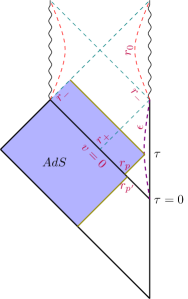
Figure 2: Penrose diagram for Vaidya AdS Reissner-Nordström spacetime. The figure is taken from [38]. The WDW patch is shown by blue color and the red dashed lines are behind the horizon cutoff. Note that due to the shock wave there is a displacement in the null boundary of WDW patch when crosses the shock wave. The displacement is shown by joint points $r_{p^{\prime}}$ and $r_{p}$ in this figure.

To compute the complexity for this model one needs to evaluate on shell action on the WDW patch depicted in the figure 2. Following our notation the null boundaries of the corresponding WDW patch are given by constant $v$ and $u$. To proceed, it is useful to decompose the WDW patch into three parts: $v<0$ and $v>0$ and $v=0$ parts. It is known that the action on null shell gives zero contribution (see e.g. [32]) and therefore we will consider two parts given by $v>0$ and $v<0$. The corresponding null boundaries of these two parts are

$$v>0 : \;\;\;\;\;\;\;\;\;\;v=0,\;\;\;\;v=\tau,\;\;\;\;\tau-v=2\int_{\epsilon}^{r(v,\tau)}\frac{dr}{f(r)},$$ (4.5)

$$v<0 : \;\;\;\;\;\;\;\;\;\;v=0,\;\;\;\;v=-\infty,\;\;\;\;r(v,\tau)=r_{p^{\prime}}(\tau)-\frac{1}{2}v\,,$$ (4.7)

where $\epsilon$ is the UV cutoff.

Actually for $v<0$ the solution is a pure AdS_d+1 solution and we will have to compute three different contributions to the on shell action that come from bulk, joint and ambiguity terms of the action. Note that since all boundaries are null their contributions are zero using the Affine parametrization to parametrize the null directions. It is then straightforward to compute the non-zero contributions. In particular for the bulk term one finds

$$I^{\rm bulk}_{v<0}=-\frac{dL^{d-1}}{8\pi G_{N}}\int d^{d-1}x\;\int_{-\infty}^{0}dv\;\int_{r_{p^{\prime}}(\tau)-\frac{1}{2}v}^{\infty}\frac{dr}{r^{d+1}}=-\frac{V_{d-1}L^{d-1}}{4\pi G_{N}}\frac{1}{d-1}\;\frac{1}{r^{d-1}_{p^{\prime}}(\tau)}.$$ (4.8)

While using the null vectors (2.17) the contribution of joint points is

$$I^{\rm joint}_{v<0}=-\frac{V_{d-1}}{8\pi G_{N}}\frac{L^{d-1}}{r_{p^{\prime}}^{d-1}(\tau)}\log\frac{\alpha\beta r^{2}_{p^{\prime}}(\tau)}{L^{2}}.$$ (4.9)

Finally one has a contribution from the ambiguity term that is

$$I^{\rm amb}=\frac{V_{d-1}L^{d-1}}{8\pi G_{N}}\left(\frac{\log\frac{\alpha\beta r_{p^{\prime}}^{2}(\tau)}{L^{2}}}{r_{p^{\prime}}^{d-1}(\tau)}+\frac{2}{(d-1)r_{p^{\prime}}^{d-1}(\tau)}\right).$$ (4.10)

Putting all terms together we find that on shell action vanishes for the $v<0$ part of WDW patch. Therefore all nonzero contributions to the on shell action come from $v>0$ part. Indeed in this part for the bulk term one has

$$I^{\rm bulk}_{v>0}=\frac{L^{d-1}}{8\pi G_{N}}\int d^{d-1}x\;\int_{0}^{\tau}dv\int_{r(v,\tau)}^{r_{-}}dr\,\left(\frac{-d}{r^{d+1}}+Q^{2}(d-2)r^{d-3}\right)=-\frac{V_{d-1}L^{d-1}}{8\pi G_{N}}\int_{0}^{\tau}dv\,\frac{f(r(v,\tau))}{r^{d}(v,\tau)}.$$ (4.11)

On the other had using the fact that $\frac{dr(v,\tau)}{d\tau}=\frac{1}{2}f(r(v,\tau))$ one can perform the above integration resulting in

$$I^{\rm bulk}_{v>0}=\frac{V_{d-1}L^{d-1}}{8\pi G_{N}}\left(\frac{2}{(d-1)r_{p}^{d-1}(\tau)}-\frac{2}{(d-1)\epsilon^{d-1}}\right)\,.$$ (4.12)

Here we have used the fact that $r(\tau,\tau)=\epsilon,r(0,\tau)=r_{p}(\tau)$. It is important to note that due to the null shock wave at $v=0$ there would be a displacement in the null boundary and the joint point $p$ is not necessary at the same point $p^{\prime}$ we have considered in the AdS part for $v<0$[32]. Of course it does not affect our results since we compute the contribution of the two parts $v<0$ and $v>0$ separately.

The $v>0$ part of the WDW has four null boundaries whose contributions to the on shell action vanish using Affine parameterization for the null directions. Therefore the remaining part needs to be computed is the contribution of joint points.

In this part of the WDW patch there are four joint points two of which are located at $r=r_{-}$, one at $r_{p}$ and one at $r=\epsilon$. Although the contributions of two later points can be easily computed using the coordinate systems we have been using so far, for those at $r_{-}$ it finds useful to utilize the following coordinate system

$$U=-e^{-\frac{1}{2}f^{\prime}(r_{-})u},\;\;\;\;\;\;\;\;\;\;V=e^{\frac{1}{2}f^{\prime}(r_{-})v},$$ (4.13)

by which the corresponding two joint points are located at $(U,V)=(\zeta,V_{0})$ and $(U,V)=(\zeta,V_{\tau})$, for $\zeta\rightarrow 0$. Denoting the $r$ coordinate associated with these points by $r_{0}$ and $r_{\tau}$, respectively, and using the normal vectors (2.17) one gets the following expression for the contribution of the joint points

$$I^{\rm joint}_{v>0}=\frac{V_{d-1}L^{d-1}}{8\pi G_{N}}\left(\frac{\log\frac{\alpha\beta r^{2}_{p}(\tau)}{L^{2}f(r_{p})}}{r_{p}^{d-1}(\tau)}-\frac{\log\frac{\alpha\beta\epsilon^{2}}{L^{2}f(\epsilon)}}{\epsilon^{d-1}}+\frac{\log\frac{\alpha\beta r^{2}_{\tau}}{L^{2}f(r_{\tau})}}{r_{\tau}^{d-1}}-\frac{\log\frac{\alpha\beta r^{2}_{0}}{L^{2}f(r_{0})}}{r_{0}^{d-1}}\,\right).$$ (4.14)

On the other hand using the fact that [39]

$$\log f(r)=\log|UV|+c_{0}+{\cal O}(UV),\;\;\;\;\;{\rm for}\;\;UV\rightarrow 0,$$ (4.15)

the above expression reads

$$I^{\rm joint}_{v>0}=\frac{V_{d-1}L^{d-1}}{8\pi G_{N}}\left(\frac{\log\frac{\alpha\beta r^{2}_{p}(\tau)}{L^{2}}}{r_{p}^{d-1}(\tau)}-\frac{\log\frac{\alpha\beta\epsilon^{2}}{L^{2}}}{\epsilon^{d-1}}-\frac{\log f(r_{p})}{r_{p}^{d-1}(\tau)}+\frac{f^{\prime}(r_{-})\tau}{2r_{-}^{d-1}}\right).$$ (4.16)

Here we have also used the fact that $\{r_{0},r_{\tau}\}\approx r_{-}$. Finally the contribution of ambiguity term is

$$I^{\rm amb}_{v>0} = \frac{V_{d-1}L^{d-1}}{8\pi G_{N}}\left(-\frac{\log\frac{\alpha r_{-}}{L}}{r_{-}^{d-1}}-\frac{1}{(d-1)r_{-}^{d-1}}+\frac{\log\frac{\alpha\epsilon}{L}}{\epsilon^{d-1}}+\frac{1}{(d-1)\epsilon^{d-1}}\right)$$ (4.21)

$$+\frac{V_{d-1}L^{d-1}}{8\pi G_{N}}\left(-\frac{\log\frac{\beta r_{p}(\tau)}{L}}{r_{p}^{d-1}(\tau)}-\frac{1}{(d-1)r_{p}^{d-1}(\tau)}+\frac{\log\frac{\beta\epsilon}{L}}{\epsilon^{d-1}}+\frac{1}{(d-1)\epsilon^{d-1}}\right)$$

$$+\frac{V_{d-1}L^{d-1}}{8\pi G_{N}}\left(-\frac{\log\frac{\alpha r_{p}(\tau)}{L}}{r_{p}^{d-1}(\tau)}-\frac{1}{(d-1)r_{p}^{d-1}(\tau)}+\frac{\log\frac{\alpha r_{-}}{L}}{r_{-}^{d-1}}+\frac{1}{(d-1)r_{-}^{d-1}}\right)$$

$$= \frac{V_{d-1}L^{d-1}}{8\pi G_{N}}\left(-\frac{\log\frac{\alpha\beta r_{p}^{2}(\tau)}{L^{2}}}{r_{p}^{d-1}(\tau)}-\frac{2}{(d-1)r_{p}^{d-1}(\tau)}+\frac{\log\frac{\alpha\beta\epsilon^{2}}{L^{2}}}{\epsilon^{d-1}}+\frac{2}{(d-1)\epsilon^{d-1}}\right).$$ (4.23)

As we already mentioned the contribution of $v<0$ part vanishes and therefore the total on shell is

$$I^{\rm total}=I^{\rm bulk}_{v>0}+I^{\rm joint}_{v>0}+I^{\rm amb}_{v>0}=\frac{V_{d-1}L^{d-1}}{8\pi G_{N}}\bigg{(}\frac{f^{\prime}(r_{-})}{2r_{-}^{d-1}}\tau-\frac{\log f(r_{p}(\tau))}{r_{p}^{d-1}(\tau)}\bigg{)}.$$ (4.24)

It is then easy to compute the time derivative of on shell action

$$\frac{dI^{\rm total}}{d\tau}=\frac{V_{d-1}L^{d-1}}{16\pi G_{N}}\left(\frac{f^{\prime}(r_{-})}{r_{-}^{d-1}}-\frac{f^{\prime}(r_{p}(\tau))}{r_{p}^{d-1}(\tau)}+\frac{d-1}{r_{p}^{d}(\tau)}f(r_{p}(\tau))\log|f(r_{p}(\tau))|\right).$$ (4.25)

Note that at late time where $r_{p}(\infty)=r_{+}$ one gets

$$\left(\frac{dI^{\rm total}}{d\tau}\right)_{\infty}=\frac{V_{d-1}L^{d-1}}{16\pi G_{N}}\left(\frac{f^{\prime}(r_{-})}{r_{-}^{d-1}}-\frac{f^{\prime}(r_{+})}{r_{+}^{d-1}}\right),$$ (4.26)

that is the same as that of eternal black brane given in the equation (2.32). It is worth mentioning that since $r_{p}\leq r_{+}$ the logarithmic term is always negative leading to the fact that the complexity growth approaches its late time value from below respecting the Lloyd’s bound. The full time dependence of complexity growth is depicted in the figure 3.

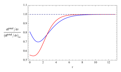
Figure 3: Rate of the complexity growth for charged Vaidya geometry with $m=1,Q=\frac{1}{3}$ (blue) and $m=1,Q=\frac{1}{10}$ (red). The growth respects the Lloyd’s bound as in the uncharged case.

Since all non-zero contributions to the on shell action come from the $v>0$ part where the geometry is essentially an AdS-RN black brane, one may also study a case where the corresponding black brane is in the stage of near extremal. Of course in order to get such a geometry the charge and the energy of infalling null matter should be fine tuned. Since in the present case the late time behavior of complexity is the same as that of two-sided black brane considered in the previous section, taking the corresponding near horizon limit would lead to the same expression given in the equation (3.7) too.

One could also try to directly compute the complexity from the near horizon solution. We note, however, that in general it is not straightforward to write a solution that is a $d+1$ dimensional AdS for $v<0$ and an AdS${}_{2}\times\mathbb{R}^{d-1}$ for $v>0$. Nonetheless as far as the computation of complexity is concerned it is possible to proceed to find the complexity for near horizon solution. Actually as we have already seen the contribution to the complexity from the $v<0$ part where we have an AdS_d-1 is zero and therefore we are left with just $v>0$ part. On the other hand in this part the geometry is the near horizon limit of near extremal case which we have considered in the previous section. Therefore we will also get the same expression for the late time behavior of complexity growth as (3.7).

It is worth noting that since the near horizon limit of the next extremal geometry results in a geometry containing an AdS₂ geometry, in order to compute the corresponding complexity the cutoff behind the horizon is required to get the correct result.

Another interesting case related to what we have considered here is to study complexity for a process of creating a near extremal RN black hole from the extremal one by adding an in falling shock wave. Such a geometry has been studied in [40].

5 Conclusions

In this paper we have studied complexity for near horizon limit of near extremal charged black brane solutions. The aim was to compute the corresponding complexity from two different approaches. In the first approach we have taken the limit from the complexity of a charged black brane while in the second approach we have computed complexity for a near horizon solution.

We have observed that in order to get the same result from both approaches one has to consider a cutoff behind the horizon whose value is given by the UV cutoff. Moreover it is crucial to add the contribution of the counter term required to have finite free energy evaluated on the cutoff surface behind the horizon.

It is also important to note that in order to find meaningful results one has to carefully take the near horizon limit of the near extremal black brane. Doing so, the resultant metric has an AdS₂ factor in the Rindler coordinates. It is worth noting that although we have computed the complexity from $d+1$ dimensional theory point of view, one could have reduced the near horizon solution into two dimensions where we would have gotten the generalized Jackiw-Teitelboim gravity (see for example [41]). The corresponding two dimensional gravity may be obtained by a dimensional reduction using the following general ansatz

$$ds^{2}=d\hat{s}_{2}^{2}+\psi^{2}\ d\vec{x}^{2}.$$ (5.1)

Plugging this metric in to the action (2.1) one gets (see e.g. [41] for more details)

$$I=\frac{V_{d-1}}{16\pi G_{N}}\int d^{2}x\sqrt{-\hat{g}_{2}}\psi^{d-1}\left(\hat{R}_{2}+(d-1)(d-2)|\hat{\nabla}\psi|^{2}\psi^{-2}+\frac{d(d-1)}{L^{2}}-\frac{1}{2}\hat{F}_{2}^{2}\right)\,.$$ (5.2)

Then the complexity could have been computed from two dimensional point of view. We note that complexity for the (generalized) Jackiw-Teitelboim gravity has been studied in [21, 10, 22]. In particular the authors of [21, 22] have studied four dimensional charged black hole reduced into two dimensions. It was shown that in order to find the desired late times linear growth for complexity the contribution of certain boundary term must be taken into account. The corresponding boundary term is ( here we have written the corresponding term for arbitrary dimensions)

$$I=\frac{1}{8\pi G_{N}}\int d^{d}x\,\sqrt{|h|}\,\,n_{\mu}F^{\mu\nu}A_{\nu}\,,$$ (5.3)

where $n_{\mu}$ is normal vector to the boundary. Actually this boundary term is the one needed to impose boundary condition on the gauge field rather than fixing the potential at the boundary. Using the equation of motion the above term may be recast to a volume term to be evaluated on the WDW patch. Interestingly enough the final result for complexity growth coincides with what we have obtained using behind the horizon cutoff. Actually it is straightforward to see that the boundary term (5.3) evaluated on the behind the horizon cutoff results in

$$I=-\frac{1}{8\pi G_{N}}\int d^{d}x\,\sqrt{|h|}\,\frac{\sqrt{h(r_{e})}}{L}\,,$$ (5.4)

that is exactly the counter terms we have considered. Of course in our picture our motivation to consider this counter term was given by the holographic renormalization It would be interesting to understand the relation between these two approaches better.

As a final remark we would like to make a comment on the behind the horizon cutoff for the charged black holes. Although in this case we have not obtained the relation between UV cutoff and the behind horizon cutoff, since for small UV cutoff we would expect that the corresponding cutoff tends to infinity where the singularity is located the behind horizon cutoff should be behind the inner horizon, as shown by red dashed lines in the left panel of figure 1 and figure 2. Therefore it does not have any direct effect in the WDW patch and thus complexity.

Indeed it is consistent with the result of [42] where a charged black hole at a finite cutoff has been studied. In this case one could see that unlike the neutral black holes the complexity is not affected by the cutoff.

On the other hand going into the near horizon the region in which the behind horizon cutoff is located will be excluded from the spacetime and we will have to reconsider the cutoff in the new coordinates denoted by $(\hat{t},\hat{r})$ in present paper. More precisely in this case the obtained spacetime has an AdS₂ factor and the corresponding cutoff is depicted by dashed red line in the right panel of figure 1.

Acknowledgments

The authors would like to kindly thank A. Akhavan, M. H. Halataei, M. R. Mohammadi Mozaffar, A. Naseh, F. Omidi, and M.H. Vahidinia for useful comments and discussions on related topics.

References

- [1] A. Almheiri, D. Marolf, J. Polchinski and J. Sully, “Black Holes: Complementarity or Firewalls?,” JHEP 1302, 062 (2013) [arXiv:1207.3123 [hep-th]].
- [2] J. M. Maldacena, “The Large N limit of superconformal field theories and supergravity,” Int. J. Theor. Phys. 38, 1113 (1999) [Adv. Theor. Math. Phys. 2, 231 (1998)] doi:10.1023/A:1026654312961, 10.4310/ATMP.1998.v2.n2.a1 [hep-th/9711200].
- [3] S. Ryu and T. Takayanagi, “Holographic derivation of entanglement entropy from AdS/CFT, ” Phys. Rev. Lett. 96, 181602 (2006) [hep-th/0603001].
- [4] L. Susskind, “Computational Complexity and Black Hole Horizons,” Fortsch. Phys. 64, 24 (2016) doi:10.1002/prop.201500092 [arXiv:1403.5695 [hep-th], arXiv:1402.5674 [hep-th]].
- [5] D. Stanford and L. Susskind, “Complexity and Shock Wave Geometries,” Phys. Rev. D 90, no. 12, 126007 (2014) doi:10.1103/PhysRevD.90.126007 [arXiv:1406.2678 [hep-th]].
- [6] A. R. Brown, D. A. Roberts, L. Susskind, B. Swingle and Y. Zhao, “Holographic Complexity Equals Bulk Action?,” Phys. Rev. Lett. 116, no. 19, 191301 (2016) doi:10.1103/PhysRevLett.116.191301 [arXiv:1509.07876 [hep-th]].
- [7] A. R. Brown, D. A. Roberts, L. Susskind, B. Swingle and Y. Zhao, “Complexity, action, and black holes,” Phys. Rev. D 93, no. 8, 086006 (2016) doi:10.1103/PhysRevD.93.086006 [arXiv:1512.04993 [hep-th]].
- [8] M. Alishahiha, K. Babaei Velni and M. R. Mohammadi Mozaffar, “Subregion Action and Complexity,” arXiv:1809.06031 [hep-th].
- [9] A. Akhavan, M. Alishahiha, A. Naseh and H. Zolfi, “Complexity and Behind the Horizon Cut Off,” JHEP 1812, 090 (2018) doi:10.1007/JHEP12(2018)090 [arXiv:1810.12015 [hep-th]].
- [10] M. Alishahiha, “On Complexity of Jackiw-Teitelboim Gravity,” arXiv:1811.09028 [hep-th].
- [11] S. Lloyd, “Ultimate physical limits to computation,” Nature 406 (2000) 1047, [arXiv:quant-ph/9908043]
- [12] D. Carmi, S. Chapman, H. Marrochio, R. C. Myers and S. Sugishita, “On the Time Dependence of Holographic Complexity,” JHEP 1711, 188 (2017) doi:10.1007/JHEP11(2017)188 [arXiv:1709.10184 [hep-th]].
- [13] R. Q. Yang, C. Niu, C. Y. Zhang and K. Y. Kim, “Comparison of holographic and field theoretic complexities for time dependent thermofield double states,” JHEP 1802, 082 (2018) doi:10.1007/JHEP02(2018)082 [arXiv:1710.00600 [hep-th]].
- [14] J. Couch, S. Eccles, W. Fischler and M. L. Xiao, “Holographic complexity and noncommutative gauge theory,” JHEP 1803, 108 (2018) doi:10.1007/JHEP03(2018)108 [arXiv:1710.07833 [hep-th]].
- [15] B. Swingle and Y. Wang, “Holographic Complexity of Einstein-Maxwell-Dilaton Gravity,” JHEP 1809, 106 (2018) doi:10.1007/JHEP09(2018)106 [arXiv:1712.09826 [hep-th]].
- [16] Y. S. An and R. H. Peng, “Effect of the dilaton on holographic complexity growth,” Phys. Rev. D 97, no. 6, 066022 (2018) doi:10.1103/PhysRevD.97.066022 [arXiv:1801.03638 [hep-th]].
- [17] M. Alishahiha, A. Faraji Astaneh, M. R. Mohammadi Mozaffar and A. Mollabashi, “Complexity Growth with Lifshitz Scaling and Hyperscaling Violation,” JHEP 1807, 042 (2018) doi:10.1007/JHEP07(2018)042 [arXiv:1802.06740 [hep-th]].
- [18] R. G. Cai, S. M. Ruan, S. J. Wang, R. Q. Yang and R. H. Peng, “Action growth for AdS black holes,” JHEP 1609, 161 (2016) doi:10.1007/JHEP09(2016)161 [arXiv:1606.08307 [gr-qc]].
- [19] A. Ovgun and K. Jusufi, “Complexity growth rates for AdS black holes with dyonic/ nonlinear charge/ stringy hair/ topological defects,” arXiv:1801.09615 [gr-qc].
- [20] E. Yaraie, H. Ghaffarnejad and M. Farsam, Eur. Phys. J. C 78, no. 11, 967 (2018) doi:10.1140/epjc/s10052-018-6456-y [arXiv:1806.07242 [gr-qc]].
- [21] A. R. Brown, H. Gharibyan, H. W. Lin, L. Susskind, L. Thorlacius and Y. Zhao, “The Case of the Missing Gates: Complexity of Jackiw-Teitelboim Gravity,” arXiv:1810.08741 [hep-th].
- [22] K. Goto, H. Marrochio, R. C. Myers, L. Queimada and B. Yoshida, “Holographic Complexity Equals Which Action?,” JHEP 02 (2019), 160 doi:10.1007/JHEP02(2019)160 [arXiv:1901.00014 [hep-th]].
- [23] K. Parattu, S. Chakraborty, B. R. Majhi and T. Padmanabhan, “A Boundary Term for the Gravitational Action with Null Boundaries,” Gen. Rel. Grav. 48, no. 7, 94 (2016) doi:10.1007/s10714-016-2093-7 [arXiv:1501.01053 [gr-qc]].
- [24] K. Parattu, S. Chakraborty and T. Padmanabhan, “Variational Principle for Gravity with Null and Non-null boundaries: A Unified Boundary Counter-term,” Eur. Phys. J. C 76, no. 3, 129 (2016) doi:10.1140/epjc/s10052-016-3979-y [arXiv:1602.07546 [gr-qc]].
- [25] L. Lehner, R. C. Myers, E. Poisson and R. D. Sorkin, “Gravitational action with null boundaries,” Phys. Rev. D 94 (2016) no.8, 084046 doi:10.1103/PhysRevD.94.084046 [arXiv:1609.00207 [hep-th]].
- [26] A. Reynolds and S. F. Ross, “Divergences in Holographic Complexity,” Class. Quant. Grav. 34, no. 10, 105004 (2017) doi:10.1088/1361-6382/aa6925 [arXiv:1612.05439 [hep-th]].
- [27] R. Emparan, C. V. Johnson and R. C. Myers, “Surface terms as counterterms in the AdS / CFT correspondence,” Phys. Rev. D 60, 104001 (1999) doi:10.1103/PhysRevD.60.104001 [hep-th/9903238].
- [28] M. Bianchi, D. Z. Freedman and K. Skenderis, “Holographic renormalization,” Nucl. Phys. B 631, 159 (2002) doi:10.1016/S0550-3213(02)00179-7 [hep-th/0112119].
- [29] A. Sen, “Quantum Entropy Function from AdS(2)/CFT(1) Correspondence,” Int. J. Mod. Phys. A 24, 4225 (2009) doi:10.1142/S0217751X09045893 [arXiv:0809.3304 [hep-th]].
- [30] K. Skenderis, “Lecture notes on holographic renormalization,” Class. Quant. Grav. 19, 5849 (2002) doi:10.1088/0264-9381/19/22/306 [hep-th/0209067].
- [31] M. Moosa, “Evolution of Complexity Following a Global Quench,” JHEP 1803, 031 (2018) doi:10.1007/JHEP03(2018)031 [arXiv:1711.02668 [hep-th]].
- [32] S. Chapman, H. Marrochio and R. C. Myers, “Holographic complexity in Vaidya spacetimes. Part I,” JHEP 1806, 046 (2018) doi:10.1007/JHEP06(2018)046 [arXiv:1804.07410 [hep-th]].
- [33] S. Chapman, H. Marrochio and R. C. Myers, “Holographic complexity in Vaidya spacetimes. Part II,” JHEP 1806, 114 (2018) doi:10.1007/JHEP06(2018)114 [arXiv:1805.07262 [hep-th]].
- [34] M. Reza Tanhayi, R. Vazirian and S. Khoeini-Moghaddam, “Complexity Growth Following Multiple Shocks,” arXiv:1809.05044 [hep-th].
- [35] Z. Y. Fan and M. Guo, “Holographic complexity under a global quantum quench,” arXiv:1811.01473 [hep-th].
- [36] D. Galante and M. Schvellinger, “Thermalization with a chemical potential from AdS spaces,” JHEP 1207, 096 (2012) doi:10.1007/JHEP07(2012)096 [arXiv:1205.1548 [hep-th]].
- [37] J. Jiang, “Holographic complexity in charged Vaidya black hole,” arXiv:1811.07347 [hep-th].
- [38] N. Callebaut, B. Craps, F. Galli, D. C. Thompson, J. Vanhoof, J. Zaanen and H. b. Zhang, “Holographic Quenches and Fermionic Spectral Functions,” JHEP 1410, 172 (2014) doi:10.1007/JHEP10(2014)172 [arXiv:1407.5975 [hep-th]].
- [39] C. A. Agon, M. Headrick and B. Swingle, “Subsystem Complexity and Holography,” arXiv:1804.01561 [hep-th].
- [40] A. Fabbri, D. J. Navarro and J. Navarro-Salas, “Quantum evolution of near extremal Reissner-Nordstrom black holes,” Nucl. Phys. B 595 (2001) 381 doi:10.1016/S0550-3213(00)00661-1 [hep-th/0006035].
- [41] D. J. Navarro, J. Navarro-Salas and P. Navarro, “Holography, degenerate horizons and entropy,” Nucl. Phys. B 580, 311 (2000) doi:10.1016/S0550-3213(00)00244-3 [hep-th/9911091].
- [42] T. Hartman, J. Kruthoff, E. Shaghoulian and A. Tajdini, “Holography at finite cutoff with a deformation,” arXiv:1807.11401 [hep-th].