$R$-MATRIX METHOD AND THE NONLOCAL NUCLEON OPTICAL POTENTIAL

Abstract

The calculable R-matrix method is applied to solve the Schrödinger equation in the optical model (OM) analysis of the elastic nucleon-nucleus scattering using a nonlocal nucleon optical potential (OP). The phenomenological nonlocal nucleon OP proposed by Perey and Buck (PB), and the two recent versions of the PB parametrization were used in the present OM study of the elastic nucleon scattering on ²⁷Al, ⁴⁰Ca, ⁴⁸Ca, ⁹⁰Zr, and ²⁰⁸Pb targets at different energies. The comparison of the OM results given by the calculable $R$-matrix method with those given by other methods confirms that the calculable $R$-matrix method is an efficient tool for the OM study of the elastic nucleon-nucleus scattering using a nonlocal nucleon OP.
Keywords: Nonlocality, nucleon optical potential, $R$-matrix method.

1 INTRODUCTION

The nucleon-nucleus scattering remains an important experiment of the modern nuclear physics to investigate the nucleon-nucleus interaction as well as the structure of the target nucleus. In particular, the elastic and inelastic scattering of the short-lived, unstable nuclei on proton target, or proton scattering in the inverse kinematics, is now extensively carried out with the secondary beams of unstable nuclei to investigate the unknown structure of unstable nuclei under study. The key quantity needed for the description of the nucleon-nucleus scattering at both low and high energies is the nucleon optical potential (OP), which determines the scattering wave function of the scattered nucleon as solution of the Schrödinger equation in a single-channel optical model (OM) or of the system of the coupled-channel (CC) equations. The elastic scattering wave function given by the OP is often dubbed as the distorted wave in the Distorted Wave Born Approximation (DWBA) or CC formalism, which are widely used to study different processes of the direct nuclear reaction [1]. Therefore, a proper treatment of the nucleon OP is always of a vital importance.

Over the years, for the simplicity of the numerical calculation, the OP was mainly assumed in the local form for the OM analysis of the elastic nucleon-nucleus scattering. The phenomenological Woods-Saxon (WS) form is mostly used in numerous parametrizations of the local nucleon OP [2, 3]. However, it is well known that the nucleon OP is nonlocal in the coordinate space due to the Pauli principle and multichannel coupling. In a microscopic theory of the nucleon OP, one can obtain the formal expression for the complex nucleon OP using the projection technique developed by Feshbach [4]

$$U=V_{0}+\lim_{\epsilon\rightarrow 0}\sum_{\alpha\alpha^{\prime}}V_{0\to\alpha}\left(\frac{1}{E-H+i\epsilon}\right)_{\alpha\alpha^{\prime}}V_{\alpha^{\prime}\to 0},$$ (1)

where the first-order term $V_{0}$ is the interaction between the incident nucleon and the target nucleus being in its ground state (g.s.), while $V_{0\to\alpha}$ is that when the target nucleus is excited to a state labeled by $\alpha$ which, in general, can be also in the continuum or a breakup channel. The first term of Eq. (1) is real and can be obtained by the folding model [5, 6, 7] as a Hartree-Fock-type potential using the realistic wave function for the target g.s. and a proper effective nucleon-nucleon interaction. If the antisymmetrization of the nucleon-nucleus system is taken exactly into account [5], then the Fock term of $V_{0}$ is nonlocal in the coordinate space. The second term of Eq. (1) is often referred to as the dynamic polarization potential (DPP), which arises from the coupling between the elastic scattering channel and the (open) nonelastic channels. The DPP is complex and nonlocal because the target nucleus that is excited at position $\bm{r}$ can return to its g.s. at another position $\bm{r}^{\prime}$, with $\bm{r}\neq\bm{r^{\prime}}$ [8]. Thus, the nonlocality of the nucleon OP has a justified physics origin and it is of importance to implement the use of the nonlocal OP in the OM, DWBA, and CC studies of the nucleon-nucleus scattering.

Although most of the OM studies of the elastic nucleon-nucleus scattering have used the local nucleon OP, several studies have been carried out using the nucleon OP in an explicit nonlocal form (see, e.g., Refs. [9, 10, 11, 12, 13]). Among them, we note the early work by Perey and Buck (PB) [9] and the recent revision of the PB parametrization by Tian, Pang, and Ma (TPM) [12], which used a nonlocal nucleon OP built up from a WS form factor multiplied by a nonlocal Gaussian. While the PB parameters were adjusted to the best OM description of the two data sets (elastic $n+^{208}$Pb scattering at 7.0 and 14.5 MeV), those of the TPM potential were fitted to reproduce the data of the elastic nucleon scattering on ³²S, ⁵⁶Fe, ¹²⁰Sn, and ²⁰⁸Pb targets at energies of 8 to 30 MeV. More recently, an energy dependence of the nonlocal OP was introduced explicitly into the imaginary parts of the PB and TPM potentials, dubbed as PB-E and TPM-E potentials, whose parameters were fitted to the best OM description of the nucleon elastic scattering data on ⁴⁰Ca, ⁹⁰Zr and ²⁰⁸Pb targets at energies $E\approx 5-45$ MeV [13, 14].

In general, solving the Schrödinger equation with a nonlocal potential readily leads to an integro-differential equation, which is more complicated than a standard differential equation with a local potential. For the nucleon-nucleus scattering problem, the use of the nonlocal OP leads to an explicit angular-momentum dependence of the integral equation for the scattering wave function. At variance with the traditional methods usually used for the integro-differential equation, we apply the calculable $R$-matrix method [15] in the present work to solve exactly the Schrödinger equation with a nonlocal nucleon OP. The recent extension of the calculable $R$-matrix method [15, 16] has included the Lagrange mesh and Gauss-Legendre quadrature integration that simplify the numerical calculation significantly. Although the $R$-matrix method was developed to treat exactly the nonlocal (central) potential, it has been applied mainly to study the nuclear resonant scattering at low energies using some local form for the scattering potential [15]. The aim of the present work is, therefore, to explore the applicability of the calculable $R$-matrix method in the OM calculation of the elastic nucleon-nucleus scattering using a nonlocal nucleon OP. For the nonlocal nucleon OP, we have chosen the PB [9] and TPM [12] potentials as well as the energy-dependent nonlocal OP by Lovell et al. [13, 14] to study the elastic nucleon scattering on ²⁷Al, ⁴⁰Ca, ⁴⁸Ca, ⁹⁰Zr, and ²⁰⁸Pb targets at energies of 14.6 MeV to 40 MeV. The OM results obtained with the calculable $R$-matrix method are compared with those obtained with other methods given by the computer codes NLOM [10, 17], NLAT [18], and DWBA98 [19].

2 Elastic nucleon scattering and the $R$-matrix method

2.1 Optical model with a nonlocal nucleon OP

We give here a brief introduction into the OM calculation with a nucleon OP that contains a nonlocal central term [9, 10, 12, 13]. In this case, the scattering wave function $\chi$ of the incident nucleon is obtained by solving the following Schrödinger equation

$$\left[-\frac{\hbar^{2}}{2\mu}\nabla^{2}+V_{\rm C}(\bm{r})+V_{\rm so}(\bm{r})\bm{l}.{\bm{\sigma}}\right]\chi(\bm{k},\bm{r})+\!\!\int V(\bm{r},\bm{r}^{\prime})\chi(\bm{k},\bm{r}^{\prime})d\bm{r}^{\prime}=E\chi(\bm{k},\bm{r}).$$ (2)

Here $V_{\rm C}(\bm{r})$ and $V_{\rm so}(\bm{r})$ are the Coulomb and spin-orbit potentials, respectively, which are assumed to be local, and $V(\bm{r},\bm{r}^{\prime})$ is the nonlocal central potential. The Coulomb potential for the incident protons is given as

$$V_{\rm C}(r)=\left\{\begin{array}[]{lcr}\displaystyle\frac{Ze^{2}}{r},&&r>R_{\rm C}\\ \displaystyle\frac{Ze^{2}}{2R_{\rm C}}\left(3-\frac{r^{2}}{R_{\rm C}^{2}}\right),&&r\leqslant R_{\rm C}.\end{array}\right.$$ (5)

The Coulomb radius $R_{\rm C}$ is determined by the mass-number dependent formula, and the spin-orbit potential $V_{\rm so}(\bm{r})$ is adopted in the usual Thomas form [2]. The wave number is determined by the reduced mass $\mu$ and center-of-mass energy $E$ as $k=\sqrt{2\mu E/\hbar^{2}}$. The spin of the incident nucleon is $\bm{s}=\hbar\bm{\sigma}/2$, where $\bm{\sigma}$ is the Pauli matrix. In the OM calculation of the elastic nucleon scattering, the orientation of the nucleon spin needs to be treated explicitly, and the scattering wave function (also dubbed as the distorted wave) is expressed [1] via the nucleon spinor $\xi$ as

$$\chi_{m_{s}}(\bm{k},\bm{r})=\sum_{m^{\prime}_{s}}\chi_{m_{s}m^{\prime}_{s}}(\bm{k},\bm{r})\xi_{\frac{1}{2}m^{\prime}_{s}},$$ (6)

where the spin matrix elements of the distorted wave are given by the following partial-wave series

$$\chi_{m_{s}m^{\prime}_{s}}(\bm{k},\bm{r})=\frac{4\pi}{kr}\sum_{ljm_{j}}\psi_{lj}(k,r)\langle l\frac{1}{2}mm_{s}|jm_{j}\rangle\langle l\frac{1}{2}m^{\prime}m^{\prime}_{s}|jm_{j}\rangle[i^{l}Y_{lm^{\prime}}(\hat{\bm{r}})]Y^{*}_{lm}(\hat{\bm{k}}).$$ (7)

Here $Y_{lm}$ are the spherical harmonics with $m=m_{j}-m_{s}$ and $m^{\prime}=m_{j}-m^{\prime}_{s}$. The nonlocal central potential can also be expanded over the spherical harmonics series as

$$V(\bm{r},\bm{r^{\prime}})=\sum_{lm}\frac{v_{l}(r,r^{\prime})}{rr^{\prime}}[i^{l}Y_{lm}(\theta,\phi)]Y^{*}_{lm}(\theta^{\prime},\phi^{\prime}).$$ (8)

Then, the radial equation for $\psi_{lj}(k,r)$ is readily obtained by multiplying both sides of Eq. (2) with the spherical harmonics $Y_{lm}(\hat{\bm{k}})$ and $Y_{lm^{\prime}}(\hat{\bm{r}})$, and integrating out the angular variables $\hat{\bm{r}}$ and $\hat{\bm{k}}$.

$$-\frac{\hbar^{2}}{2\mu}\left[\frac{d^{2}}{dr^{2}}-\frac{l(l+1)}{r^{2}}\right]\psi_{lj}(k,r)+\left[V_{\rm C}(r)+A_{lj}V_{\rm so}(r)\right]\psi_{lj}(k,r)$$

$$+\int v_{l}(r,r^{\prime})\psi_{lj}(k,r^{\prime})dr^{\prime}=E\psi_{lj}(k,r),$$ (9)

where $A_{lj}=l$ when $j=l+\frac{1}{2}$, and $A_{lj}=-l-1$ when $j=l-\frac{1}{2}$. The spin matrix elements $\chi_{m_{s}m^{\prime}_{s}}(\bm{r},\bm{k})$ of the distorted wave obtained from the solutions $\psi_{lj}(k,r)$ of Eq. (2.1) can be expressed in terms of the Coulomb $\chi_{\rm C}$ and scattered $\chi_{\rm scatt}$ waves as

$$\chi_{m_{s}m^{\prime}_{s}}(\bm{k},\bm{r})=\chi_{\rm C}(\bm{k},\bm{r})\delta_{m_{s}m^{\prime}_{s}}+\chi_{\text{scatt},m_{s}m^{\prime}_{s}}(\bm{k},\bm{r}),$$ (10)

and $\chi_{\text{scatt},m_{s}m^{\prime}_{s}}$ has the following asymptotic form

$$\chi_{\text{scatt},m_{s}m^{\prime}_{s}}(\bm{k},\bm{r})\sim\frac{e^{i(kr-\eta\ln 2kr)}}{r}f_{m_{s}m^{\prime}_{s}}(\theta),$$ (11)

where $f_{m_{s}m^{\prime}_{s}}(\theta)$ are the spin matrix elements of the elastic scattering amplitude, $\eta$ is the usual Coulomb parameter. Matching $\psi_{lj}$ with the corresponding term of the Coulomb wave function at large radii, where the nuclear potential is negligible, we obtain the scattering phase shift $\delta_{l}^{\pm}$. Then, the partial-wave elements of the scattering matrix ($S_{lj}=S_{l}^{+}$ with $j=l+\frac{1}{2}$, and $S_{lj}=S_{l}^{-}$ with $j=l-\frac{1}{2}$) are determined by the relation

$$S_{l}^{\pm}=\exp({2i\delta_{l}^{\pm}}).$$ (12)

The amplitude of the elastic nucleon-nucleus scattering can be expressed in terms of an operator $\bm{f}$ acting on the spin of the incident nucleon [1] as

$$\bm{f}(\theta)=g(\theta)\bm{1}+ih(\theta)\bm{\sigma}.\bm{n},$$ (13)

where $\bm{n}$ is the unit vector along the direction $\bm{k}\times\bm{k^{\prime}}$, which is perpendicular to the scattering plane. We further adopt the frame with the $z$-axis aligned along $\bm{k}$, and the $y$-axis along $\bm{n}$. Then the spin matrix elements of $\bm{f}$ can be expressed as

$$f_{++}=f_{--}=g(\theta),f_{+-}=-f_{-+}=h(\theta),$$ (14)

where the subscript $\pm$ denotes $m_{s}=\pm\frac{1}{2}$. The explicit expressions for $g(\theta)$ and $h(\theta)$ functions are [1]

$$g(\theta)=f_{\rm C}(\theta)+\frac{i}{2k}\sum_{l}[(2l+1)-(l+1)S^{+}_{l}-lS^{-}_{l}]\exp(2i\sigma_{l})P^{0}_{l}(\cos\theta)$$

$$h(\theta)=\frac{i}{2k}\sum_{l}(S^{-}_{l}-S^{+}_{l})\exp(2i\sigma_{l})P^{1}_{l}(\cos\theta),$$ (15)

where $f_{\rm C}(\theta)$ and $\sigma_{l}$ are the Rutherford scattering amplitude and Coulomb phase shift, respectively, and $P^{0(1)}_{l}(\cos\theta)$ are the Legendre polynomials. Finally, the differential scattering cross section for the elastic (unpolarized) nucleon scattering is obtained as

$$\frac{d\sigma(\theta)}{d\Omega}=\frac{1}{2}\sum_{m_{s}m^{\prime}_{s}}|f_{m_{s}m^{\prime}_{s}}(\theta)|^{2}=|g(\theta)|^{2}+|h(\theta)|^{2}.$$ (16)

2.2 The calculable $R$-matrix method

The calculable $R$-matrix method introduced in Ref. [15] is an efficient tool to solve the scattering problem using the Schödinger equation. It is different from the phenomenological $R$-matrix method which is a technique to parametrize the cross section of the nuclear resonant scattering. The main principle of solving the Schrödinger Eq. (2.1) using the calculable $R$-matrix method is the division of the configuration space at the channel radius $a$ into an internal region and an external region. The channel radius $a$ is chosen large enough so that the nuclear potential is negligible in the external region. In the present work, $a=15fm$ was chosen for all the OM calculations using the $R$-matrix method. The partial-wave component $\psi_{lj}(r)$ of the scattering wave function in the external region can then be written as

$$\psi_{lj}^{\rm ext}(r)=\frac{i}{2}\left[I_{l}(kr)-S_{lj}O_{l}(kr)\right],$$ (17)

with the conjugate functions $I_{l}$ and $O_{l}$ determined as

$$I_{l}=G_{l}-iF_{l},\ O_{l}=G_{l}+iF_{l},$$ (18)

where $F_{l}$ and $G_{l}$ are the regular and irregular Coulomb functions, respectively. In the internal region, the wave function is expanded over some finite basis of $N$ linearly independent function $\varphi_{n}$ as

$$\psi_{lj}^{\rm int}(r)=\sum_{n=1}^{N}c_{n}\varphi_{n}(r).$$ (19)

The internal and external parts of the radial wave function can be connected at the boundary $r=a$ through the continuity condition $\psi^{\rm{int}}_{lj}(a)=\psi^{\rm{ext}}_{lj}(a)=\psi_{lj}(a)$. This leads to the definition of the $R$-matrix at a given energy $E$ as

$$\psi_{lj}(a)=\mathscr{R}_{lj}(E)[a\psi^{{}^{\prime}}_{lj}(a)-B\psi_{lj}(a)],$$ (20)

where $B$ is the dimensionless boundary parameter introduced for the later convenience. The $R$-matrix has dimension 1 in the single-channel case and is just a function of energy $E$. Because the Hamiltonian is not Hermitian over the internal region $(0,a)$, the following surface Bloch operator [20] is introduced

$$\mathscr{L}(B)=\frac{\hbar^{2}}{2\mu}\delta(r-a)\left(\frac{d}{dr}-\frac{B}{r}\right),$$ (21)

so that the combination of the Hamiltonian and Bloch operator is Hermitian over the region $(0,a)$ when $B$ is real. It is well known that for the scattering problem, the results obtained using the $R$-matrix method are independent of $B$ [15]. Therefore, we have fixed $B=0$ in the present work, and the Schrödinger equation in the internal region can be approximated by an inhomogeneous Bloch-Schrödinger equation. Eq. (2.1) can then be rewritten as

$$\left\{-\frac{\hbar^{2}}{2\mu}\left[\frac{d^{2}}{dr^{2}}+\frac{l(l+1)}{r^{2}}\right]+V_{\rm C}(r)+A_{lj}V_{\rm so}(r)-E+\mathscr{L}\right\}\sum_{i=1}^{N}c_{n}\varphi_{n}(r)$$

$$+\int v_{l}(r,r^{\prime})\sum_{i=1}^{N}c_{n}\varphi_{n}(r^{\prime})dr^{\prime}=\mathscr{L}\psi_{lj}^{\rm ext}(r).$$ (22)

The Bloch operator $\mathscr{L}$ ensures the continuity of the derivative of the wave function. Projecting both sides of Eq. (22) on $\varphi_{i}(r)$ and integrating over $r$ variable, we obtain

$$\sum_{n=1}^{N}C_{in}(E)c_{n}=\frac{\hbar^{2}}{2\mu}\varphi_{i}(a)\frac{d\psi_{lj}^{\rm ext}(r)}{dr}\Big{|}_{\displaystyle{r=a}},$$ (23)

where the matrix elements $C_{in}(E)$ are determined as

$$C_{in}(E)\!\!\! = \!\!\!\!\!\int\varphi_{i}(r)\Big{\{}-\frac{\hbar^{2}}{2\mu}\left[\frac{d^{2}}{dr^{2}}+\frac{l(l+1)}{r^{2}}\right]+V_{\rm C}(r)+A_{lj}V_{\rm so}(r)$$ (24)

$$\!\!\!\!\!-E+\mathscr{L}\Big{\}}\varphi_{n}(r)dr+\int\varphi_{i}(r)v_{l}(r,r^{\prime})\varphi_{n}(r^{\prime})drdr^{\prime}.$$

The coefficients $c_{n}$ are obtained by solving the system of linear equations (23). Inserting them into Eq. (19) at $r=a$ and using the boundary condition (20), we obtain the calculable $R$-matrix

$$\mathscr{R}_{lj}(E)=\frac{\hbar^{2}}{2\mu a}\sum_{i,n=1}^{N}\varphi_{i}(a)(C^{-1})_{in}\varphi_{n}(a).$$ (25)

For the convenience in the calculation of $C_{in}(E)$, the modified Lagrange functions are chosen as the basis functions $\varphi_{n}(r)$ (see the explicit expressions in Ref. [15]). Using the Gauss-Legendre quadrature, the integral of any regular function can be approximated by a sum of the function values at the mesh points $\{r_{i}\}$ given by the solutions of the Legendre polynomial, multiplied by the weight $\lambda_{i}$ in the interval $[0,a]$. Then, the basic functions satisfy the Lagrange condition [15],

$$\varphi_{n}(r_{i})=(\lambda_{i})^{-1/2}\delta_{in}.$$ (26)

Thanks to the relation (26), the calculation is simplified significantly and we obtain for the all local potentials in Eq. (24)

$$\int_{0}^{a}\varphi_{i}(r)V(r)\varphi_{n}(r)dr=\sum_{k=1}^{N}\lambda_{k}\varphi_{i}(r_{k})V(r_{k})\varphi_{n}(r_{k})=V(r_{i})\delta_{in},$$ (27)

and for the nonlocal central potential

$$\int\varphi_{i}(r)v_{l}(r,r^{\prime})\varphi_{n}(r^{\prime})dr^{\prime}dr=v_{l}(r_{i},r_{n}).$$ (28)

Thus, the calculable $R$-matrix method allows us to obtain the solution of the scattering equation (22) with a nonlocal central potential without using an iterative procedure. It is obvious that external wave functions contain the partial-wave elements $S_{lj}$ of the scattering matrix and internal wave functions which include the $R$-matrix component $\mathscr{R}_{lj}(E)$. Through the continuity condition of the scattering wave function, the relationship between $S_{lj}$ and $\mathscr{R}_{lj}(E)$ is obtained as

$$S_{lj}=\exp(2i\phi_{l})\frac{1-L_{l}^{*}\mathscr{R}_{lj}(E)}{1-L_{l}}\mathscr{R}_{lj}(E),$$ (29)

where

$$L_{l}=\frac{ka}{O_{l}(ka)}\frac{dO_{l}(kr)}{dr}\Big{|}_{\displaystyle{r=a}}$$

is the dimensionless logarithmic derivative of $O_{l}$ at the channel radius $a$, and

$$\phi_{l}=\arg I_{l}(ka)=-\arctan\left[\frac{F_{l}(ka)}{G_{l}(ka)}\right]$$ (30)

is the hard-sphere Coulomb phase shift. The differential scattering cross section (16) for the elastic (unpolarized) nucleon scattering is then readily obtained from the partial-wave elements of the scattering matrix (29)

2.3 The nonlocal nucleon OP

To explore the use of the calculable $R$-matrix method, we adopt in the present work the phenomenological nonlocal nucleon OP proposed by Perey and Buck [9] for the neutron elastic scattering from ²⁰⁸Pb target at the energies of 7.0 and 14.5 MeV. The original PB parameters have been improved recently by Tian, Pang, and Ma [12] to reproduce the elastic nucleon scattering data on ³²S, ⁵⁶Fe, ¹²⁰Sn, and ²⁰⁸Pb targets at the energies of 8 to 30 MeV. Like the original PB potential that consists of a nonlocal real volume term, a nonlocal imaginary surface term, and a local real spin-orbit potential, the TPM potential includes further a nonlocal imaginary volume term. More recently, the energy dependence of the nonlocal OP has been introduced explicitly into the imaginary parts of the PB and TPM potentials (the PB-E and TPM-E potentials) based on the OM fit to the neutron elastic scattering data on ⁴⁰Ca, ⁹⁰Zr, and ²⁰⁸Pb targets at the energies of 5 to 40 MeV [13]. All these versions of the nonlocal nucleon OP were parametrized in the following form

$$V(\bm{r},\bm{r^{\prime}})=U\left(\frac{|\bm{r}+\bm{r^{\prime}}|}{2}\right)H\left(\frac{|\bm{r}-\bm{r^{\prime}}|}{\beta}\right),$$ (31)

where $\beta$ is the range of the nonlocality. The function $H(|\bm{r}-\bm{r^{\prime}}|/\beta)$ was chosen [9] in the Gaussian form

$$H\left(\frac{|\bm{r}-\bm{r^{\prime}}|}{\beta}\right)=\frac{1}{\pi^{\frac{3}{2}}\beta^{3}}\exp\left[-\left(\frac{\bm{r}-\bm{r^{\prime}}}{\beta}\right)^{2}\right],$$ (32)

and the function $U(p)$ with $p=|\bm{r}+\bm{r^{\prime}}|/2$ was chosen in the Woods-Saxon form like those usually used [2] for the local OP

$$-U(p)=V_{\rm R}f_{\rm R}(p)+iW_{\rm I}f_{\rm I}(p)+iW_{\rm D}f_{\rm D}(p),$$ (33)

where

$$f_{\rm R(I)}(p) = \left[1+\exp\left(\frac{p-R_{\rm R(I)}}{a_{\rm R(I)}}\right)\right]^{-1}$$ (34)

$$f_{\rm D}(p) = 4\exp\left(\frac{p-R_{\rm D}}{a_{\rm D}}\right)\left[1+\exp\left(\frac{p-R_{\rm D}}{a_{\rm D}}\right)\right]^{-2}.$$

$R_{i}=r_{i}A^{1/3}$ and $a_{i}$ ($i={\rm R,I,D}$) are the potential radius and diffuseness tabulated in Refs. [9, 12, 13]. Because of the dominant contribution of the Gaussian factor to the integral at $\bm{r}\approx\bm{r^{\prime}}$, the approximation $p=|\bm{r}+\bm{r^{\prime}}|/2\approx(r+r^{\prime})/2$ is made [9] to simplify the computation of $v_{l}(r,r^{\prime})$. Then, one obtains

$$v_{l}(r,r^{\prime})=U\left(\frac{r+r^{\prime}}{2}\right)\frac{1}{\pi^{\frac{1}{2}}\beta}\exp\left[-\frac{(r^{2}+r^{\prime 2})}{\beta^{2}}\right]2i^{l}zj_{l}(-iz),$$ (35)

where $z=2rr^{\prime}/\beta^{2}$ and $j_{l}(x)$ is the spherical Bessel function. The Schrödinger equation (2.1) using the nonlocal potential (22) for the elastic nucleon scattering can be solved numerically by the traditional methods or by the calculable $R$-matrix method discussed above.

3 RESULTS AND DISCUSSION

Before presenting the OM results obtained with the calculable $R$-matrix method, it is of interest to discuss briefly the iterative method used in the OM calculations with the nonlocal nucleon OP. In these calculations, a trial local potential $U_{\text{init}}$ is used to generate the initial scattering wave function for the iteration scheme [9]

$$\frac{\hbar^{2}}{2\mu}\left[\frac{d^{2}}{dr^{2}}-\frac{l(l+1)}{r^{2}}\right]\psi^{(0)}_{lj}(r)+\left[E-V_{\rm C}(r)-A_{lj}V_{\rm so}(r)-U_{\text{init}}(r)\right]\psi^{(0)}_{lj}(r)=0.$$ (36)

The solution $\psi^{(0)}_{lj}(r)$ given by the initial local potential is then used in the first step ($n=1$) of solving the integro-differential equation iteratively

$$\frac{\hbar^{2}}{2\mu}\left[\frac{d^{2}}{dr^{2}}-\frac{l(l+1)}{r^{2}}\right]\psi^{(n)}_{lj}(r)+\left[E-V_{\rm C}(r)-A_{lj}V_{\rm so}(r)-U_{\text{init}}(r)\right]\psi^{(n)}_{lj}(r)$$

$$=\int v_{l}(r,r^{\prime})\psi^{(n-1)}_{lj}(r^{\prime})dr^{\prime}-U_{\text{init}}(r)\psi^{(n-1)}_{lj}(r).$$ (37)

Such an iterative procedure performs as many iterations as necessary for the convergence of the scattering wave function. Although the choice of $U_{\text{init}}(r)$ does not affect the final solution of the scattering equation, the convergence of the iterative method somewhat depends on the choice of the initial local potential. In the study of the nucleon transfer reactions by Titus et al. [18, 21], the iterative method has been used to determine both the scattering and bound nucleon wave functions (the code NLAT).

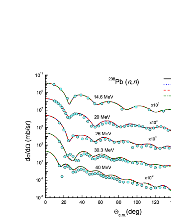
Figure 1: OM descriptions of the neutron elastic scattering on ²⁰⁸Pb target at 14.6, 20, 26, 30.3 and 40 MeV given by the calculable $R$-matrix method and other methods (see detailed discussion in text) using the nonlocal PB potential [9]. The experimental data were taken from Refs. [22, 23, 24, 25, 26].

The NLOM method [10, 17] was suggested to solve the nonlocal OM equation quickly and reliably, using the Green-function transformation to convert the scattering wave function to the form of a bound-state wave function that can be expanded over an orthonormal basis. Then the main problem is to solve a set of the inhomogeneous linear equations using, e.g., the Lanczos method which also needs an iterative procedure. In this method, the trial local potential is still necessary, but the convergence is not sensitive to the chosen trial potential.

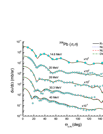
Figure 2: The same at Fig. 1 but using the nonlocal TPM potential [12]. The experimental data were taken from Refs. [22, 23, 24, 25, 26].

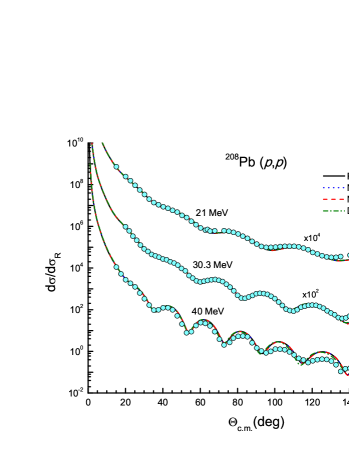
Figure 3: OM descriptions of the proton elastic scattering on ²⁰⁸Pb target at 21, 30.3, and 40 MeV given by the calculable $R$-matrix method and other methods (see detailed discussion in text) using the nonlocal TPM potential [12]. The experimental data were taken from Refs. [27, 28].

Another way of solving the integro-differential equation (2.1) is to divide the radial variable into the equal mesh points $\{r_{k}\}$, and to express the derivative and integral in terms of the wave function $\psi_{lj}(r_{k})$ at the mesh points. The integro-differential equation is then transformed to a set of the linear equations

$$D_{ik}\psi_{lj}(r_{k})=0,$$ (38)

where the coefficients $D_{ik}$ are determined from the expansion of the second derivative and nonlocal integral over the full set of $\psi_{lj}(r_{k})$. This method has been implemented by Raynal in the DWBA98 code [19] for the elastic and inelastic nucleon scattering.

At variance with these methods, the nonlocality of the nucleon OP is treated directly in the calculable $R$-matrix method without involving the intermediate steps of an iterative method or using some specific transformation of the nonlocal term. Another advantage of the $R$-matrix method is the use of the Lagrange-mesh method that allows the direct determination of the local (27) and nonlocal (28) matrix elements. In the present work, we have tested the reliability of the calculable $R$-matrix method by comparing the OM results given by the $R$-matrix method with those given by the three methods discussed above. Fig. 1 presents the OM descriptions of the neutron elastic scattering on ²⁰⁸Pb target at the energies of 14.6, 20, 26, 30.3, and 40 MeV given by the four different methods of solving Eq. (2.1), using the same nonlocal PB potential [9]. One can see that all the considered methods give nearly the same differential scattering cross sections over the whole angular range, which are indistinguishable in the logarithmic scale. In the case of the TPM potential [12], a nonlocal imaginary volume term was added and all the parameters have been fitted to give a proper OM description of the elastic neutron and proton scattering over a wide range of energies. From the OM results for the elastic angular distribution of the neutron and proton elastic scattering on ²⁰⁸Pb target shown in Fig. 2 and Fig 3 one can see that the calculable $R$-matrix method also reproduces the OM results given by the three referred methods.

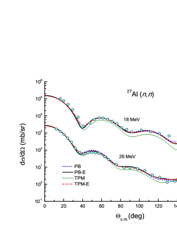
Figure 4: OM descriptions of the neutron elastic scattering on ²⁷Al target at the energies of 18 and 26 MeV given by the calculable $R$-matrix method using the nonlocal PB and TPM potentials [9, 12] and their energy dependent PB-E and TPM-E versions [13]. The experimental data were taken from Ref. [29].

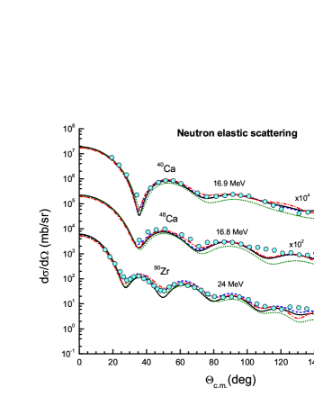
Figure 5: OM descriptions of the neutron elastic scattering on ⁴⁰Ca, ⁴⁸Ca, and ⁹⁰Zr targets at the energies of 16.9, 16.8, and 24 MeV respectively by the calculable $R$-matrix method using the nonlocal PB and TPM potential [9] and its energy dependent version [13]. The experimental data were taken from Refs. [30, 31, 32].

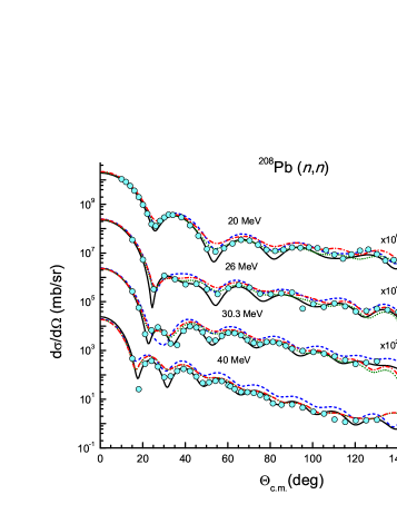
Figure 6: OM descriptions of the neutron elastic scattering on ²⁰⁸Pb target at the energies of 20, 26, 30.3, and 40 MeV given by the calculable $R$-matrix method using the nonlocal PB and TPM potential [9] and its energy dependent version [13]. The experimental data were taken from Refs. [23, 24, 25, 26].

Because the parameters of the PB potential were fitted to reproduce the data of the neutron elastic scattering on ²⁰⁸Pb target at energies below 15 MeV, it gives a worse OM description of the data at higher energies. That is the reason the parameters of the TPM potential were searched [12] to obtain a good OM description of the elastic nucleon scattering data at the energies of around 10 to 30 MeV. Our OM results have shown that the TPM potential indeed gives a better OM description of the neutron elastic scattering data at 30.3 and 40 MeV (compare the lower parts of Fig. 1 and Fig. 2). From the microscopic point of view, the imaginary part of the nucleon OP originates mainly from the couplings between the elastic scattering channel and open nonelastic channels, expressed through the dynamic polarization term in Eq. (1). Because DPP is strongly nonlocal and energy dependent, it is necessary to include an explicit energy dependence into the imaginary part of the PB and TPM nonlocal potentials as done recently by Lovell et al. [13], where the energy dependent parameters of the OP were adjusted to fit the neutron elastic scattering data on ⁴⁰Ca, ⁹⁰Zr, and ²⁰⁸Pb targets at the energies of 5 to 40 MeV (see PB-E and TPM-E parameters in Table II of Ref. [13]). The OM results obtained with the calculable $R$-matrix method for the neutron elastic scattering on ²⁷Al, ⁴⁰Ca, ⁴⁸Ca, ⁹⁰Zr, and ²⁰⁸Pb targets at the energies of 16.8 to 40 MeV using the original PB, TPM potentials and their energy dependent PB-E, TPM-E versions are compared with the data in Fig. 4, Fig. 5, and Fig. 6. In all cases, the energy dependent PB-E and TPM-E nonlocal potentials give a better OM description of the data compared to the original PB and TPM potential, especially, in Fig. 4 the good description of the data for ²⁷Al is obtained at both energies although these data sets were not included in the OM search of the energy dependent OP parameters in Ref. [13]. In Fig. 5, the energy dependent nonlocal potentials also give a better OM description of the data for ⁴⁰Ca, ⁴⁸Ca, and ⁹⁰Zr compared to the original PB and TPM potentials, this behavior is more clearly seen by the TPM-E potential compared to TPM potential. The similar result is obtained in Fig. 6, where one can see the improved description of the data by the energy dependent PB-E nonlocal potential at the energies of 30.3 and 40 MeV.

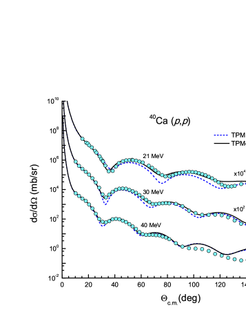
Figure 7: OM descriptions of the proton elastic scattering on ⁴⁰Ca target at the energies of 21, 30, and 40 MeV given by the calculable $R$-matrix method using the nonlocal TPM potential [12] and its energy dependent TPM-E version [14]. The experimental data were taken from Refs. [33].

Recently, the energy dependent version TPM-E has been extended to the OM study of the elastic proton scattering on ⁴⁰Ca, ⁹⁰Zr, and ²⁰⁸Pb targets at energies of E $\approx$ 10$-$45 MeV [14]. We have used here the TPM nonlocal potentials and the new energy dependent TPM-E version in the OM calculation of the proton elastic scattering on ⁴⁰Ca target at 21, 30, and 40 MeV by the $R$-matrix method. One can see in Fig. 7 that the energy dependent TPM-E nonlocal potentials also give a better OM description of the data at three energies compared to the original TPM potential.

Summary

The applicability of the calculable $R$-matrix method in the OM calculation of the elastic nucleon scattering with a nonlocal nucleon OP has been explored in the OM analysis of the elastic nucleon scattering on ²⁷Al, ⁴⁰Ca, ⁴⁸Ca, and ²⁰⁸Pb targets at the incident energies up to 40 MeV, using the phenomenological nonlocal nucleon OP proposed by Perey and Buck [9], and the two recent versions of the PB parametrization [12, 13, 14].

The comparison of the OM results given by the calculable $R$-matrix method [15] with those given by the three other methods [17, 18, 19] confirms that the calculable $R$-matrix method is an efficient, alternative method to treat the nonlocality of the nucleon OP. The direct evaluation of the nonlocal term of the OP based on the Lagrange-mesh method can be applied further in the OM study using the microscopic nucleon OP given by the folding model calculation that treats the nonlocal exchange term exactly [5].

Based on the present results, it should be possible to use the nonlocal, microscopic nucleon-nucleus potential in the $R$-matrix study of the nucleon radiative capture at the astrophysical energies. This will be the subject of our upcoming research.

References

- [1] G. R. Satchler, Direct Nuclear Reactions, Clarendon Press Oxford, New York (1983).
- [2] R. L. Varner, W. J. Thompson, T. L. McAbee, E. J. Ludwig, and T. B. Clegg, Phys. Rep., 201 (1991) 57.
- [3] A. Koning and J. Delaroche, Nucl. Phys. A, 713 (2003) 231.
- [4] H. Feshbach, Theoretical Nuclear Physics, Vol. II, Wiley, New York, (1992).
- [5] K. Amos, P. J. Dortmans, S. Karataglidis, H. V. von Geramb, and J. Raynal, Adv. Nucl. Phys., 25 (2001) 275.
- [6] F. A. Brieva, and J. R. Rook, Nucl. Phys. A, 291 (1977) 299; Nucl. Phys. A, 291 (1977) 317.
- [7] D. T. Khoa, E. Khan, G. Colò, and N. V. Giai, Nucl. Phys. A, 706 (2002) 61.
- [8] M. E. Brandan and G. R. Satchler, Phys. Rep., 285 (1997) 143.
- [9] F. Perey and B. Buck, Nucl. Phys., 32 (1962) 353.
- [10] B. T. Kim and T. Udagawa, Phys. Rev. C, 42 (1990) 1147.
- [11] K. Minomo, K. Ogata, M. Kohno, Y. R. Shimizu, and M. Yahiro, J. Phys. G, 37 (2010) 085011.
- [12] Y. Tian, D. Y. Pang, and Z. Y. Ma, Int. J. Mod. Phys. E, 24 (2015) 1550006.
- [13] A. E. Lovell, P. L. Bacq, P. Capel, F. M. Nunes, and L. J. Titus, Phys. Rev. C, 96 (2017) 051601(R).
- [14] M. I. Jaghoub, A. E. Lovell, and F. M. Nunes, Phys. Rev. C, 98 (2018) 024609.
- [15] P. Descouvemont and D. Baye, Rep. Prog. Phys., 73 (2010) 36301.
- [16] P. Descouvemont, Comp. Phys. Comm., 200 (2016) 199.
- [17] B. T. Kim, M.C. Kyum, S. W. Hong, M. H. Park, and T. Udagawa, Comp. Phys. Comm., 71 (1992) 150.
- [18] L. J. Titus, A. Ross, and F. M. Nunes, Comp. Phys. Comm., 207 (2016) 499.
- [19] J. Raynal, Computing as a Language of Physics, IAEA, Vienna (1972) p.75; Notes on DWBA98 code (unpublished).
- [20] B. A. Robson, Nucl. Phys. A, 132 (1969) 5.
- [21] L. J. Titus, F. M. Nunes, and G. Potel, Phys. Rev. C, 93 (2016) 014604.
- [22] L. F. Hansen, F. S. Dietrich, B. A. Pohl, C. H. Poppe, and C. Wong, Phys. Rev. C, 31 (1985) 111.
- [23] R. W. Finlay, J. R. M. Annand, T. S. Cheema, J. Rapaport, and F. S. Dietrich, Phys. Rev. C, 30 (1984) 796.
- [24] J. Rapaport, T. S. Cheema, D. E. Bainum, R. W. Finlay, and J. D. Carlson, Nucl. Phys. A, 313 (1979) 1.
- [25] R. P. DeVito, Sam M. Austin, W. Sterrenburg, and U. E. P. Berg, Phys. Rev. Lett., 47 (1981) 628.
- [26] R. P. DeVito, D. T. Khoa, S. M. Austin, U. E. P. Berg, and B. M. Loc, Phys. Rev. C, 85 (2012) 024619.
- [27] W. T. H. van Oers, Huang Haw, N. E. Davison, A. Ingemarsson, B. Fagerström, and G. Tibell, Phys. Rev. C, 10 (1974) 307.
- [28] L. N. Blumberg, E. E. Gross, A. VAN DER Woude, A. Zucker, and R. H. Bassel, Phys. Rev., 147 (1966) 812.
- [29] J. S. Petler, M. S. Islam, R. W. Finlay, and F. S. Dietrich, Phys. Rev. C, 32 (1985) 673.
- [30] G. M. Honoré, W. Tornow, C. R. Howell, R. S. Pedroni, R. C. Byrd, R. L. Walter, and J. P. Delaroche, Phys. Rev. C, 33 (1986) 1129.
- [31] J. M. Mueller, R. J. Charity, R. Shane, L. G. Sobotka, S. J. Waldecker, W. H. Dickhoff, A. S. Crowell, J. H. Esterline, B. Fallin, C. R. Howell, C. Westerfeldt, M. Youngs, B. J. Crowe, III, and R. S. Pedroni, Phys. Rev. C, 83 (2011) 064605.
- [32] Y. Wang and J. Rapaport, Nuclear Physics A, 517 (1990) 301.
- [33] R. H. McCamis, T. N. Nasr, J. Birchall, N. E. Davison, W. T. H. van Oers, P. J. T. Verheijen, R. F. Carlson, A. J. Cox, B. C. Clark, E. D. Cooper, S. Hama, and R. L. Mercer, Phys. Rev. C, 33 (1986) 1624.