Pseudo-Implicit Feedback for Alleviating Data Sparsity in Top-K Recommendation

Abstract

We propose PsiRec, a novel user preference propagation recommender that incorporates pseudo-implicit feedback for enriching the original sparse implicit feedback dataset. Three of the unique characteristics of PsiRec are: (i) it views user-item interactions as a bipartite graph and models pseudo-implicit feedback from this perspective; (ii) its random walks-based approach extracts graph structure information from this bipartite graph, toward estimating pseudo-implicit feedback; and (iii) it adopts a Skip-gram inspired measure of confidence in pseudo-implicit feedback that captures the pointwise mutual information between users and items. This pseudo-implicit feedback is ultimately incorporated into a new latent factor model to estimate user preference in cases of extreme sparsity. PsiRec results in improvements of 21.5% and 22.7% in terms of Precision@10 and Recall@10 over state-of-the-art Collaborative Denoising Auto-Encoders. Our implementation is available at https://github.com/heyunh2015/PsiRecICDM2018.

I Introduction

We focus on the problem of top-K recommendation under conditions of extreme sparsity in implicit feedback datasets. The goal of top-K item recommendation is to generate a list of $K$ items for each user, typically by modeling the hidden preferences of users toward items based on the set of actual user-item interactions. While implicit feedback (like clicks, purchases) is often more readily available than explicit feedback, in many cases it too suffers from sparsity since users may only interact with a small subset of all items, leading to poor quality recommendation.

Typically, there are two main strategies to alleviate the interaction sparsity problem. The first is to adopt a latent factor model to map users and items into the same low-rank dimensional space [1, 2, 3, 4, 5, 6]. The second is to propagate user preferences using random walks to “nearby” items so that direct user-item pairs can propagate to transitive user-item pairs [7, 8, 9, 10, 11]. In this paper, we propose a novel approach that combines the advantages of both latent factor and random walk models.

Our key intuition is to carefully model pseudo-implicit feedback from the larger space of indirect, transitive user-item pairs and embed this feedback in a latent factor model. Concretely, we propose PsiRec, a novel user preference propagation recommender that incorporates pseudo-implicit feedback for enriching the original sparse implicit feedback dataset. This pseudo-implicit feedback can naturally be estimated through an embedding model which we show explicitly factorizes a matrix where each entry is the pointwise mutual information value of a user and item in our sample of pseudo user-item pairs. We show how this pseudo-implicit feedback corresponds to random walks on the user-item graph. To model confidence in pseudo-implicit feedback, we adopt a Skip-gram [12] inspired measure that captures the pointwise mutual information between users and items.

Experiments over sparse Amazon and Tmall datasets show that our approach outperforms matrix factorization approaches as well as more sophisticated neural network approaches and effectively alleviates the data sparsity problem. Further, we observe that the sparser the datasets are, the larger improvement can be obtained by capturing the pseudo-implicit feedback from indirect transitive relationships among users and items.

II Related Work

There is a rich line of research on top-K recommendation for implicit feedback datasets [1, 3, 4, 5, 6], where typically positive examples are extremely sparse. One family of approaches enriches the interactions between users and items via exploring the transitive, indirect associations that are not observed in the training data [7, 8, 9, 10, 11]. Huang et al. [7] compute the association between a user and an item as the sum of the weights of all paths connecting them. ItemRank [8] employs PageRank on the correlation graph between items to infer the preference of a user. $P^{3}$ [13] ranks items according to the third power of the transition matrix.

As another line of research, latent factor (LF) models learn to assign each user a vector of latent user factors and each item with a vector of latent item factors. These dense latent factors enable similarity computations between arbitrary pairs of users and items, and thus can address the data sparsity problem. As a representative type of LF models, matrix factorization (MF) methods model the preference of user $u$ over item $i$ as the inner product of their latent representations [1, 2]. In terms of optimization, they aim to minimize the squared loss between the predicted preferences and the ground-truth preferences. A number of works can be seen as a variation of MF methods by employing different models to learn the user-item interaction function [3, 6] or using different loss functions [4, 14]. Our method brings together these two lines of research by exploiting both direct and indirect associations between users and items with a matrix factorization model.

III Preliminaries

Let $U$ and $I$ denote the set of users and items respectively. Additionally, let $M$ and $N$ represent the number of users and items. We also reserve $u$ to represent a user and $i$ to represent an item. We define the user-item interaction matrix as $\textbf{R}\in\mathbb{R}^{M\times N}$, and denote the implicit feedback from $u$ on $i$ as $r_{ui}$. In many cases, implicit feedback datasets only contain the logs of binary interactions where $r_{ui}=1$ indicates $u$ purchased $i$ and $r_{ui}=0$ the otherwise. Therefore, we focus on binary interactions in this paper. Non-binary interactions can be handled with slight modifications to our approach. Based on these interactions, top-K item recommendation generates a list of $K$ items for each user, where each item $i$ is ranked by the (hidden) preference of $u$, denoted as $p_{ui}$. The preference matrix for all users and items is denoted as $\textbf{P}\in\mathbb{R}^{M\times N}$.

One traditional approach [2] for estimating this user preference is through latent factor models like matrix factorization. We define $\textbf{x}_{u}$ to be the latent factor vector for $u$ and $\textbf{y}_{i}$ to be the latent factor vector for $i$. Matrices $\textbf{X}\in\mathbb{R}^{M\times K}$ and $\textbf{Y}\in\mathbb{R}^{N\times K}$ represent the latent factor matrix for users and items accordingly. User preferences can be estimated as the following inner product: $\hat{p}_{ui}=\textbf{x}_{u}^{T}\textbf{y}_{i}$. Model parameters can then be learned by minimizing the squared error between $r_{ui}$ and $\hat{p}_{ui}$: $\ell=\sum_{u,i}(r_{ui}-\hat{p}_{ui})^{2}$. However, in case of extremely sparse user-item interactions, even such latent factor models may face great challenges: the number of direct user-item pairs ($r_{ui}=1$) may be too few to learn meaningful latent factors.

IV PsiRec: Pseudo-Implicit Feedback

In this section, we propose a general approach for enhancing top-K recommenders with pseudo-implicit feedback. Our key intuition is that the original sparse interaction matrix R can be enriched by carefully modeling transitive relationships to better estimate user preference. Concretely, our approach can be divided into steps given as follows:

• First, we view the user-item interactions as a bipartite graph and propose to model pseudo-implicit feedback from this perspective.

• Second, we propose a random walks-based approach to extract evidence of user-item closeness from this bipartite graph toward estimating pseudo-implicit feedback.

• Third, we describe two strategies to measure the confidence of pseudo-implicit feedback based on these sampled user-item pairs from the bipartite graph.

• Finally, we develop a latent factor model to estimate user preference from this pseudo-implicit feedback.

IV-A Pseudo-Implicit Feedback

Complementary to viewing the user-item interactions as a matrix, we can view R as a bipartite graph $G=(V,E)$, where $V=U\cup I$ and there exists an edge $e_{ui}\in E$ if and only if $r_{ui}=1$. Figure 1 presents a toy example of $G$, where a circle represents a user and a rectangle represents an item.

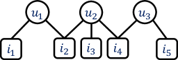
Figure 1: A toy example of the user-item bipartite graph $G$. A circle represents a user and a rectangle represents an item.

From this perspective, we hypothesize that there are many cases where $u$ probably likes $i$ even though $u$ never purchases $i$. For example, in Figure 1, $u_{1}$ and $u_{2}$ both purchased $i_{2}$, which implies that $u_{1}$ and $u_{2}$ probably share some similarities in their preference patterns. The fact that $u_{1}$ purchased $i_{1}$ indicates that $u_{1}$ probably likes $i_{1}$. Since $u_{1}$ and $u_{2}$ have similar preferences, $u_{2}$ probably likes $i_{1}$ so that he might also purchase $i_{1}$. Hence, we propose to treat these indirect relationships as evidence of pseudo-implicit feedback. Intuitively, the more distance between the user and the item in the graph, the less confidence we have in the pseudo-implicit feedback. Formally, we define pseudo-implicit feedback as:

Definition 1.

Pseudo-Implicit Feedback. Pseudo-implicit feedback is a non-negative real-valued implicit feedback from $u$ to $i$, denoted as $s_{ui}\in\mathbb{R}_{\geq 0}$. The larger $s_{ui}$ is, the higher confidence on the pseudo-implicit feedback from $u$ to $i$ is. If $u$ and $i$ are connected through a path in $G$, then $s_{ui}>0$. The pseudo-implicit feedback matrix is denoted by S.

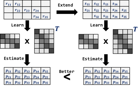
Figure 2: A toy example of generating pseudo-implicit feedback S from original implicit feedback R (based on Figure 1) to better estimate user preference P on very sparse datasets.

Figure 2 provides a toy example based on the user-item bipartite graph in Figure 1. Clearly, S is denser than R since it also incorporates indirect user-item pairs in $G$. Then, we still follow the above-mentioned latent factor model to estimate user preferences: $\hat{p}_{ui}=x_{u}^{T}y_{i}$. The model parameters $x_{u}$ and $y_{i}$ can be learned by minimizing $\ell=\sum_{u,i}(s_{ui}-\hat{p}_{ui})^{2}$. In this way, we can leverage the pseudo-implicit feedback from indirect user-item pairs to alleviate the data sparsity problem.

The key question, then, is how to generate S, the pseudo-implicit feedback matrix? Care must be taken to capture meaningful (pseudo) user-item pairs without also incorporating spurious, noise-inducing user-item pairs. Hence, we propose to generate the pseudo-implicit feedback matrix by exploiting a Skip-gram inspired approach that captures user-item closeness in the bipartite graph. Specifically, we propose to estimate S through two steps: (1) The first step is to extract user-item pairs from the graph $G$. Recall that according to Definition 1, if $i$ is reachable by $u$, then $s_{ui}>0$. Hence, we need to sample these (pseudo) user-item pairs; and (2) then measure the confidence of this feedback based on the sampled user-item pairs. Straightforward co-occurrence counts from these random walk samples is a first step, but may miss subtleties of user-item pairs not occurring in the sample. Hence, we propose a neural embedding model to overcome this challenge.

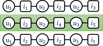
(a) Generated random walks.

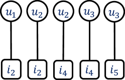
(b) Direct pairs.

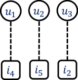
(c) Indirect pairs.

Figure 3: Figure 3(a) shows three random walks starting from $u_{1}$ in Figure 1. Figure 3(b) and Figure 3(c) show the direct user-item pairs and indirect user-item pairs sampled from the second random walk in Figure 3(a) when the window size is 3.

IV-B Random Walks to Extract User-Item Pairs

Inspired by previous works like DeepWalk [15], we propose to use truncated random walks to sample user-item pairs in the user-item bipartite graph. Recall that a random walk is a stochastic process with random variables. Concretely, a truncated random walk can be represented as a linear sequence of vertices $v_{i}$, $v_{i+1}$,…,$v_{i+\gamma}$, where ${v_{i+k}}$ is a vertex sampled uniformly from the neighbors of ${v_{i+k-1}}$. For each vertex $v_{i}\in V=U\cup I$, we launch $\beta$ walks of length $\gamma$ on $G$, forming the set of random walks $\mathcal{W}$. We use $\mathcal{W}_{v_{i}}$ to represent a random walk starting from vertex $v_{i}$.

Algorithm 1 Sample $(u,i)$ from the random walks $\mathcal{W}$

Input: User set $U$, item set $I$, random walks $\mathcal{W}$, window size $\sigma$
    Output: The set of $(u,i)$.

1:  $C=\emptyset$

2:  for each $\mathcal{W}_{v_{i}}\in\mathcal{W}$  do

3:     for each $\mathcal{W}_{v_{i}}^{j}\in\mathcal{W}_{v_{i}}$ and $\mathcal{W}_{v_{i}}^{j}\in U$ do

4:        for each $k\in[j-\sigma:j+\sigma:2]$ do

5:           $C=C\cup(\mathcal{W}_{v_{i}}^{j},\mathcal{W}_{v_{i}}^{k})$

6:        end for

7:     end for

8:  end for

Once the corpus of random walks $\mathcal{W}$ is obtained, we sample user-item pairs from it as presented in Algorithm 1. In Lines 2-3, we iterate over all users in all random walk sequences. For each user vertex ($v\in U$) in the sequences, any item vertex ($v\in I$) whose distance from $v$ is not greater than the window size will be sampled. An example of the output of Algorithm 1 is shown in Figure 3(a), where we sample three random walks starting from $u_{1}$ in the graph presented in Figure 1. Figure 3(b) and Figure 3(c) show the direct and indirect user-item pairs sampled from the second random walk in Figure 3(a) when the window size is set to 3.

IV-C Measuring Pseudo-Implicit Feedback

The next question is how to measure the pseudo-implicit feedback $s_{ui}$ from the sampled user-item pairs above. In this subsection, we investigate two strategies for estimating $s_{ui}$ for each $(u,i)$ pair: co-occurrence counts and pointwise mutual information (PMI) [16]. Our approach using the two strategies are denoted as PsiRec-CO and PsiRec-PMI respectively. We first discuss the co-occurrence counts strategy. After that, to overcome its limitation, the latter one is presented as well as its connection to the well-known Skip-gram embedding model. The comparison of their performance will be discussed in Section V-D.

IV-C1 Co-occurrence counts

Let $(u,i)$ represents a pair of $u$ and $i$. One straightforward measurement of $s_{ui}$ is the total number of times $(u,i)$ appear in $C$:

$$s_{ui}=\#(u,i)$$ (1)

However, this measurement suffers from the drawback that $\#(u,i)$ is strongly influenced by the popularity (i.e. vertex degree) of users and items. As a consequence, for most users high degree items will dominate their recommendations [11]. Similarly, for most items, their co-occurrence count with the high degree users will be large. The deeper reason behind this drawback is that it only considers the positive samples – the user-item pairs appearing in $C$, but ignores the negative samples – the user-item pairs not appearing in $C$.

IV-C2 Pointwise mutual information

To overcome this limitation, we first build an embedding model to measure $s_{ui}$ and then further propose an improved version of the model which explicitly factorizes a matrix where each entry is the pointwise mutual information (PMI) value of $u$ and $i$ in $C$. Motivated by the Skip-gram with negative sampling (SGNS) model [12], we aim to maximize the probability of observing the user-item pairs that appear in the corpus $C$ and minimize the probability of observing pairs that do not appear in $C$. We denote the embedding vector for user $u$ as $\vec{u}$ and the embedding vector for item $i$ as $\vec{i\vphantom{b}}$. The probability that $(u,i)$ is from $C$ is:

$$P(D=1|u,i)=\sigma(\vec{u\vphantom{b}}\cdot\vec{i\vphantom{b}})=\frac{1}{1+e^{-\vec{u\vphantom{b}}\cdot\vec{i\vphantom{b}}}}$$

For each positive example, we then draw several random items $i_{N}$ from the set of items $I$ as negative examples. Since the randomly drawn items are unlikely to co-occur with $u$, we want to minimize the probability of observing these $(u,i_{N})$ pairs. The training objective for a single $(u,i)$ observation is:

$$\log\sigma(\vec{u\vphantom{b}}\cdot\vec{i\vphantom{b}})+k\cdot\mathbb{E}_{i_{N}\sim P_{D}}[\log\sigma(-\vec{u\vphantom{b}}\cdot\vec{i_{N}\vphantom{b}})]$$ (2)

where $k$ is the number of negative samples and $i_{N}$ is a random item drawn according to a distribution $P_{D}$ over $I$. Here, following SGNS, we use $P_{D}=\frac{\#(i)}{|C|}$ where $\#(i)$ is the number of occurrences of $i$ in $C$. The global training objective can be defined over all $(u,i)\in C$:

$$\ell=\sum_{(u,i)\in C}(\log\sigma(\vec{u\vphantom{b}}\cdot\vec{i\vphantom{b}})+k\cdot\mathbb{E}_{i_{N}\sim P_{D}}[\log\sigma(-\vec{u\vphantom{b}}\cdot\vec{i_{N}\vphantom{b}})])$$ (3)

which can be optimized with stochastic gradient descent.

However, the above embedding model fails to take advantage of the large amount of repetitions in $C$. A user-item pair may have hundreds or thousands of occurrences in the corpus, incurring a large time cost for model training. Thus, a natural question to ask is: can we directly operate on the co-occurrence statistics of the user-item corpus? To answer this question, inspired by [17], we first re-write the loss function in Eq. 3 w.r.t each unique user-item pair:

$$\begin{array}[]{l}\ell=\sum_{u\in U}\sum_{i\in I}\#(u,i)(\log\sigma(\vec{u\vphantom{b}}\cdot\vec{i\vphantom{b}})+\\ k\cdot\#(u)\cdot\mathbb{E}_{i_{N}\sim P_{D}}[\log\sigma(-\vec{u\vphantom{b}}\cdot\vec{i_{N}\vphantom{b}})])\end{array}$$ (4)

Additionally, we explicitly express the expectation term $\mathbb{E}_{i_{N}\sim P_{D}}[\log\sigma(-\vec{u\vphantom{b}}\cdot\vec{i_{N}\vphantom{b}})]$ as follows:

$$\begin{array}[]{l}\mathbb{E}_{i_{N}\sim P_{D}}[\log\sigma(-\vec{u\vphantom{b}}\cdot\vec{i_{N}\vphantom{b}})]=\\ \frac{\#(i)}{|C|}\log\sigma(-\vec{u\vphantom{b}}\cdot\vec{i\vphantom{b}})+\sum\limits_{i_{N}\in I\backslash\{i\}}\frac{\#(i_{N})}{|C|}\log\sigma(-\vec{u\vphantom{b}}\cdot\vec{i_{N}\vphantom{b}})\end{array}$$ (5)

Combining Eq. 4 and Eq. 5 leads to a local loss for a specific user-item pair $(u,i)$:

$$\ell(u,i)=\#(u,i)\log\sigma(\vec{u\vphantom{b}}\cdot\vec{i\vphantom{b}})+k\cdot\#(u)\cdot\frac{\#(i)}{|C|}\log\sigma(-\vec{u\vphantom{b}}\cdot\vec{i\vphantom{b}})$$ (6)

Let $s^{\prime}_{ui}=\vec{u\vphantom{b}}\cdot\vec{i\vphantom{b}}$. We then take the derivative of Eq. 6 w.r.t. $s^{\prime}_{ui}$ and set it to zero, which eventually leads to:

$$s^{\prime}_{ui}=\vec{u\vphantom{b}}\cdot\vec{i\vphantom{b}}=\log(\frac{\#(u,i)\cdot|C|}{\#(u)\cdot\#(i)})-\log k$$ (7)

We note that the term $\log(\frac{\#(u,i)\cdot|C|}{\#(u)\cdot\#(i)})$ is the pointwise mututal information (PMI) of $(u,i)$, which is widely used to measure the association between random variables. This indicates that the objective function in Eq. 3 is implicitly factorizing a user-item association matrix, where each entry is the PMI of $(u,i)$ shifted by a constant $\log k$.

However, we notice that the above formulation of $s^{\prime}_{ui}$ has a problem: for $(u,i)$ pairs that never appear in $C$, their PMI are ill-defined since $\#(u,i)=0$. Moreover, it is suggested that $(u,i)$ pairs with very low or even negative PMI scores are less informative and should be discarded [18]. Thus, we propose to compute $s_{ui}$ by applying the following transformation:

$$s_{ui}=\max(s^{\prime}_{ui},0)$$ (8)

This formulation of $s_{ui}$ assigns zeros to both $(u,i)$ pairs that do not appear in $C$ and those with very low or negative PMI values, thus, solving both problems above. In addition, S is a non-negative matrix which is consistent with Definition 1.

IV-D Latent Factor Model to Estimate User Preference

Finally, we propose a matrix factorization approach to estimate $p_{ui}$ based on the learned pseudo-implicit feedback matrix $S$, where the loss function is:

$$\ell=\sum_{u,i}(s_{ui}-\textbf{x}_{u}^{T}\textbf{y}_{i})^{2}+\lambda(\sum_{u}||\textbf{x}_{u}||^{2}+\sum_{i}||\textbf{y}_{i}||^{2})$$ (9)

where $\lambda$ controls the strength of regularization to prevent overfitting. Inspired by [1], we apply the well-known Alternating Least Square (ALS) algorithm to optimize the loss function in Eq. 9. Let $\textbf{s}_{u}\in\mathbb{R}^{N}$ represents the pseudo-implicit feedback over all items of $u$ and $\textbf{s}_{i}\in\mathbb{R}^{M}$ represents the pseudo-implicit feedback of $i$ over all users. By setting $\frac{\partial\ell}{\partial\textbf{x}_{u}}=0$ and $\frac{\partial\ell}{\partial\textbf{y}_{i}}=0$, we have:

$$\textbf{x}_{u}=(\textbf{Y}^{T}\textbf{Y}+\lambda\textbf{D})^{-1}\textbf{Y}^{T}\textbf{s}_{u}$$ (10)

$$\textbf{y}_{i}=(\textbf{X}^{T}\textbf{X}+\lambda\textbf{D})^{-1}\textbf{X}^{T}\textbf{s}_{i}$$ (11)

where D represents the identity matrix. After X and Y are learned, the whole predicted preference matrix $\hat{\textbf{P}}\in\mathbb{R}^{M\times N}$ is reconstructed by $\hat{\textbf{P}}=\textbf{X}^{T}\textbf{Y}$, where $\hat{p}_{ui}$ is used to rank items.

V Experimental Evaluation

V-A Datasets and Evaluation Metrics

Amazon. The Amazon dataset contains explicit feedback, where users give a rating from 1 to 5 on the purchased items. Following previous work [1, 6], we transform these explicit datasets into implicit datasets by treating all ratings as 1, indicating that the user has purchased the item.

Tmall. The Tmall dataset contains anonymized shopping logs of customers on Tmall.com. Originally, the dataset consists of different types of user implicit feedback, such as clicks, add-to-cart actions, and purchases. For our experiments, we focus on the purchase action logs and transform them into the binary interactions R since these are closely aligned with our purchase prediction task. Further, we filter out users and items with fewer than 20 interactions.

Table I summarizes the basic statistics of these two datasets. Note that the densities of the two datasets are 0.072% and 0.051% respectively. We also observe that even after performing the filtering on the Tmall dataset described above that it is still the sparser one.

For our experiments, we randomly split each dataset into three parts: 80% for training, 10% for validation (for parameter tuning only) and 10% for testing (for evaluation). Since many users have very few interactions, they may not appear in the testing set at all. In this case, there will be no match between the top-K recommendations of any algorithm and the ground truth since there are no further purchases made by these users. The results reported here include these users, reflecting the challenges of recommendation under extreme sparsity.

TABLE I: Summary statistics for the evaluation datasets

Dataset	Users	Items	Interactions	Density	$\frac{Interactions}{User}$
Amazon Toys	19,412	11,924	167,597	0.072%	8.63
Tmall	28,291	28,401	410,714	0.051%	14.51

Metrics. Given a user, a top-K item recommendation algorithm provides a ranked list of items according to the predicted preference for each user. To assess the ranked list with respect to the ground-truth item set of what users actually purchased, we adopt three evaluation metrics: precision@k, recall@k, and F1@k, where we average each metric across all users.

V-B Baselines

ItemPop. This simple method recommends the most popular items to all users, where items are ranked by the number of times they are purchased.

BPR [4]. Bayesian personalized ranking (BPR) is a standard pairwise ranking framework for implicit recommendation.

MF [2]. Traditional matrix factorization (MF) method uses mean squared error as the objective function with negative sampling from the non-observed items ($r_{ui}=0$).

NCF [6]. Neural collaborative filtering (NCF) is a state-of-the-art neural network recommender. NCF concatenates latent factors learned from a generalized matrix factorization model and a multi-layered perceptron model and then use a regression layer to predict user preferences.

CDAE [3]. Collaborative Denoising Auto-Encoders (CDAE) is another successful neural network approach for top-K recommendation. A standard Denoising Auto-Encoder takes R as input and reconstructs it with an auto-encoder. CDAE extends the standard Denoising Auto-Encoder by also encoding a user latent factor.

V-C Hyperparameter Settings

Our preliminary experiments show that a large number of latent factors can be helpful for learning user preferences on sparse datasets. Hence, for all methods, we set the number of latent factors to 100. For all baseline methods, we carefully choose the other hyperparameters over the validation set.

Particularly, for our approach, the regularization parameter $\lambda$ is 0.25, the number of random walks $\beta$ for each node is 10. The length $\gamma$ of each random walk is 80. The window size $\sigma$ for sampling the user-item pairs is 3.

V-D Comparison between the Two Strategies for Measuring S

We first compare the performance of PsiRec-CO and PsiRec-PMI. The results in Table II, III show that PMI is significantly superior to co-occurrence as the measure of pseudo-implicit feedback. The higher the degree of a vertex in the user-item bipartite graph, the higher probabilities of the vertex co-occurring with other vertices. Hence, a high $\#(u,i)$ might not guarantee a high confidence if $\#(i)$ or $\#(u)$ is also very large. Therefore, it is more reasonable to let $\#(u,i)$ to be normalized by the global frequency of $u$ and $i$, which is exactly what PMI captures. Since PsiRec-PMI brings considerable improvements upon PsiRec-CO, we focus on PsiRec-PMI for the rest of this paper.

V-E Comparison with Baselines

Tables II, III also show the experimental results of the baseline methods, along with the improvement of PsiRec-PMI over the strongest baseline CDAE. Statistical significance was tested by the t-test, where “*” denotes statistical significance at $p=0.01$ level.

On both datasets, we observe that PsiRec-PMI significantly outperforms all baseline methods on all metrics. For instance, PsiRec-PMI achieves the best P@10 of 0.728% and 0.978% on the two datasets, representing 20.5% and 26.8% improvement upon the strongest baseline method CDAE. Similarly, significant improvements in terms of recall are also observed. PsiRec-PMI achieves this by combining pseudo-implicit feedback with a simple matrix factorization model, which is much more scalable and easier to tune than the state-of-the-art neural network methods. The experimental results demonstrate that, on sparse datasets, matrix factorization method largely benefits from considering indirectly transitive user-item relationships, and pseudo-implicit feedback generated by PsiRec-PMI can better estimate the users’ actual preferences.

TABLE II: Experimental Results on Amazon Toys and Games

Metric(%)	P@5	R@5	F1@5	P@10	R@10	F1@10
ItemPop	0.127	0.412	0.194	0.112	0.753	0.195
BPR	0.183	0.616	0.283	0.159	1.087	0.277
MF	0.533	1.716	0.813	0.403	2.532	0.695
NCF	0.733	2.529	1.136	0.531	3.565	0.924
CDAE	0.801	2.727	1.238	0.604	4.044	1.051
PsiRec-CO	0.633	2.100	0.972	0.495	3.249	0.859
PsiRec-PMI	$0.955^{*}$	$3.224^{*}$	$1.474^{*}$	$0.728^{*}$	$4.824^{*}$	$1.265^{*}$
Improvement(%)	+19.3	+18.2	+19.1	+20.5	+19.3	+20.3

TABLE III: Experimental Results on Tmall

Metric(%)	P@5	R@5	F1@5	P@10	R@10	F1@10
ItemPop	0.168	0.436	0.243	0.150	0.775	0.251
BPR	0.245	0.574	0.344	0.209	0.965	0.343
MF	1.010	2.466	1.433	0.646	3.124	1.071
NCF	0.747	1.914	1.074	0.537	2.730	0.897
CDAE	1.126	2.877	1.619	0.771	3.955	1.291
PsiRec-CO	1.142	2.773	1.618	0.732	3.556	1.214
PsiRec-PMI	$1.444^{*}$	$3.663^{*}$	$2.072^{*}$	$0.978^{*}$	$4.952^{*}$	$1.633^{*}$
Improvement(%)	+28.2	+27.3	+28.0	+26.8	+25.2	+26.5

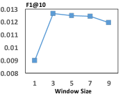
(a) Interactions Kept: $100\%$

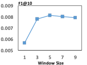
(b) Interactions Kept: $80\%$

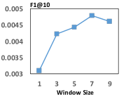
(c) Interactions Kept: $60\%$

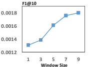
(d) Interactions Kept: $40\%$

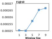
(e) Interactions Kept: $20\%$

Figure 4: Impact of the window size on Amazon Toys and Games dataset and its four sparser versions.

V-F Robustness of PsiRec-PMI on Very Sparse Datasets

We further evaluate the effectiveness of PsiRec-PMI as the degree of data sparsity increases. Keeping the same set of users and items, four sparser versions of the Amazon Toys and Games dataset are generated by randomly removing 20%, 40%, 60% and 80% purchases for each user. Particularly, Figure 5 shows that the sparser the datasets are, the larger improvements in terms of F1@10 are achieved upon the strongest baseline CDAE. This demonstrates the promising ability of PsiRec to alleviate the data sparsity problem.

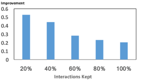
Figure 5: Improvements (F1@10) of PsiRec upon CDAE on Amazon Toys and Games and its four sparser versions.

V-G Impact of Window Size

V-G1 Effectiveness of Transitive User-Item Relationship

In the user-item bipartite graph, indirectly connected user-item pairs will be sampled by our random walks only if $\sigma>=3$. Figure 4 shows the performance of PsiRec-PMI as we vary this window size on the Amazon Toys and Games dataset and its four sparser versions. We observe that the optimal result in terms of F1@10 is always achieved when $\sigma>=3$, with a considerable improvement upon $\sigma=1$ on all datasets. This indicates that, on sparse datasets, indirectly connected user-item pairs can significantly enhance matrix factorization methods for top-K recommendation.

V-G2 Optimal Window Size on Sparse Datasets

The impact of the window size on PsiRec-PMI on Amazon Toys dataset and its four sparser versions is shown in Figure 4. There are two observations: (1) The performance is sensitive to the window size on all datasets; and (2) The sparser the dataset is, the larger the optimal window size is. Specifically, the optimal window size for datasets keeping percentage: 100%, 80%, 60%, 40% and 20% are 3, 5, 7, 9, 9 respectively. This suggests that the sparser the dataset, a larger window size is needed to sample more and longer transitive user-item relationships to enrich S so that the user preferences can be better estimated.

VI Conclusions and Future Work

We propose PsiRec, a user preference propagation recommender designed to alleviate the data sparsity problem in top-K recommendation for implicit feedback datasets. Extensive experiments show that the proposed matrix factorization method significantly outperforms several state-of-the-art neural methods, and that introducing indirect relationships leads to a large boost in top-K recommendation performance. In the future, we aim to improve PsiRec by exploring pairwise learners and the impact of incorporating side information like review text and temporal signals.

References

- [1] Y. Hu, Y. Koren, and C. Volinsky, “Collaborative filtering for implicit feedback datasets,” in ICDM, 2008.
- [2] Y. Koren, R. Bell, and C. Volinsky, “Matrix factorization techniques for recommender systems,” Computer, 2009.
- [3] Y. Wu, C. DuBois, A. X. Zheng, and M. Ester, “Collaborative denoising auto-encoders for top-n recommender systems,” in WSDM, 2016.
- [4] S. Rendle, C. Freudenthaler, Z. Gantner, and L. Schmidt-Thieme, “Bpr: Bayesian personalized ranking from implicit feedback,” in UAI, 2009.
- [5] R. Pan, Y. Zhou, B. Cao, N. N. Liu, R. Lukose, M. Scholz, and Q. Yang, “One-class collaborative filtering,” in ICDM, 2008.
- [6] X. He, L. Liao, H. Zhang, L. Nie, X. Hu, and T.-S. Chua, “Neural collaborative filtering,” in WWW, 2017.
- [7] Z. Huang, H. Chen, and D. Zeng, “Applying associative retrieval techniques to alleviate the sparsity problem in collaborative filtering,” TOIS, 2004.
- [8] M. Gori, A. Pucci, V. Roma, and I. Siena, “Itemrank: A random-walk based scoring algorithm for recommender engines.” in IJCAI, 2007.
- [9] H. Yildirim and M. S. Krishnamoorthy, “A random walk method for alleviating the sparsity problem in collaborative filtering,” in Recsys, 2008.
- [10] M. Jamali and M. Ester, “Trustwalker: a random walk model for combining trust-based and item-based recommendation,” in KDD, 2009.
- [11] F. Christoffel, B. Paudel, C. Newell, and A. Bernstein, “Blockbusters and wallflowers: Accurate, diverse, and scalable recommendations with random walks,” in Recsys, 2015.
- [12] T. Mikolov, I. Sutskever, K. Chen, G. S. Corrado, and J. Dean, “Distributed representations of words and phrases and their compositionality,” in NIPS, 2013.
- [13] C. Cooper, S. H. Lee, T. Radzik, and Y. Siantos, “Random walks in recommender systems: exact computation and simulations,” in WWW, 2014.
- [14] J. D. Rennie and N. Srebro, “Fast maximum margin matrix factorization for collaborative prediction,” in ICML, 2005.
- [15] B. Perozzi, R. Al-Rfou, and S. Skiena, “Deepwalk: Online learning of social representations,” in KDD, 2014.
- [16] K. W. Church and P. Hanks, “Word association norms, mutual information, and lexicography,” Computational linguistics, 1990.
- [17] O. Levy and Y. Goldberg, “Neural word embedding as implicit matrix factorization,” in NIPS, 2014.
- [18] J. A. Bullinaria and J. P. Levy, “Extracting semantic representations from word co-occurrence statistics: A computational study,” Behavior research methods, 2007.