Acceleration due to buoyancy and mass renormalization

Abstract

The acceleration of a light buoyant object in a fluid is analyzed. Misconceptions about the magnitude of that acceleration are briefly described and refuted. The notion of the added mass is explained and the added mass is computed for an ellipsoid of revolution. A simple approximation scheme is employed to derive the added mass of a slender body. The slender-body limit is non-analytic, indicating a singular character of the perturbation due to the thickness of the body. An experimental determination of the acceleration is presented and found to agree well with the theoretical prediction. The added mass illustrates the concept of mass renormalization in an accessible manner.

I Introduction

Imagine holding a piece of cork under water. When released, it surges towards the surface. What is its acceleration? This should be an easy question, at least when the cork is still moving slowly so that drag can be neglected. Surprisingly, textbooks and practicing physicists express a spectrum of conflicting opinions.

Some physics textbooks(YF14, ; meirovitch2010fundamentals, ) suggest that the mass of the body $m_{b}$ alone determines its acceleration $a$ due to the balance of the forces of buoyancy $F_{B}$ and weight $m_{b}g$. This suggests an arbitrarily large acceleration if the water density greatly exceeds the density of the cork. For a partially submerged cork on the surface, very large frequency of small oscillations follows, too.

Another point of view accounts for the water that has to move to make room for the accelerating cork: as the cork proceeds upwards, an equal volume of water accelerates downwards. The two accelerations have opposite signs but equal magnitudes. It is tempting to conclude that this magnitude cannot exceed the standard gravitational acceleration $g$, since “the maximum acceleration for the displaced fluid is the free fall acceleration.”(physicsmyths, ) Although this statement is not completely accurate, accounting for the fluid’s acceleration motivates the concept of added mass: in Newton’s law $a=\left(F_{B}-m_{b}g\right)/m$, the mass of the displaced fluid $m_{f}$ supplements the cork mass in some measure,

$$m=m_{b}+C_{{\scriptscriptstyle M}}m_{f},$$ (1)

with a dimensionless added-mass coefficient $C_{{\scriptscriptstyle M}}$. George Green first introduced the concept of added mass, in the context of submerged pendulums, about two centuries ago.(GeorgeGreenPapers, )

Added mass in a fluid is analogous to the mass renormalization of subatomic particles, as pointed out by Sydney Coleman in his famous, yet unpublished, quantum field theory lectures.(Connes-Motives, ) The increased inertia of a body immersed in fluid is similar to the charged particle mass modified by an interaction with a gauge field. Moreover, the subatomic particle mass renormalization depends on its surroundings, be it perfect vacuum, a cavity, or an atomic bound state. Similarly, the added mass changes in the proximity of a wall or of the fluid surface. Both phenomena are non-dissipative.

This analogy is pedagogically valuable: it is not trivial to develop an intuition for the mass generation of a subatomic particle, due to the Higgs field and the charge-selfinteraction. The elementary particle context is shrouded in mathematical intricacies, sometimes including divergent integrals. It easier to explain how a body can be weighed outside a fluid and how its inertia is modified in a fluid. In fact, even a divergent integral will be encountered when some degrees of freedom are ignored (see Section II).

For a sphere, the added mass amounts to half of the mass of the fluid it displaces (see Appendix A), as has been demonstrated in a beautiful recent experiment.(messer:2010aa, ; pantaleone:2011aa, ) This value of $C_{{\scriptscriptstyle M}}=\frac{1}{2}$ leads to the maximum surge acceleration of twice $g$, if the mass of the displaced fluid far exceeds the body mass, as in the case of a ping-pong ball under water. This leads to a third misconception, namely that $2g$, following from the buoyancy force acting both on the body and on the fluid it displaces, is the maximum acceleration of a surging body, independent of its shape.

The present paper is intended to popularize the notion of the added mass. A theoretical argument in Section II shows that the acceleration can significantly exceed $2g$, and that acceleration does indeed depend on the geometry of the body and on its orientation. In addition to a detailed exact calculation for a prolate ellipsoid (Appendix B), the simple calculation in Section II is found to reproduce the leading added-mass effect of a slender body. An experimental proof of high acceleration is presented in Section III, and may be easily reproduced in a classroom or on a field trip to a lake.

II Simple derivation of the added mass

When a slender body is moving with velocity $\bm{v}$ with respect to a fluid, the fluid parts to make room for it, then closes behind the body. The resulting fluid motion is predominantly perpendicular to $\bm{v}$ (transversal). We denote the fluid’s kinetic energy by $T$.

Consider an elongated (prolate) ellipsoid of revolution with the long semi-axis $c$ and two equal short semi-axes $b<c$. Define the slenderness parameter $\epsilon=b/c$. If the body is slender, $\epsilon\ll 1$, and moving along $c$, $T$ is small in the sense that it vanishes with $\epsilon$: when the body is collapsed into a line, its motion does not disturb the fluid. However, this limit will turn out to be nontrivial, involving both a power and a logarithm of $\epsilon$. The thickness of a slender body is an example of a singular perturbation.(historySingPert, )

In order to determine $T$, consider the velocity distribution of the fluid shown in Figure 1. The long axis of the ellipsoid lies on the $z$-axis and the origin of the coordinate system is at the center of the ellipsoid. Transverse directions are parametrized by the azimuthal angle $\varphi$ and the distance $r$ from the $z$-axis. The boundary of the ellipsoid is axisymmetric and described by $r=R\left(z\right)$,

$$\left(\frac{z}{c}\right)^{2}+\left(\frac{R\left(z\right)}{b}\right)^{2}=1.$$ (2)

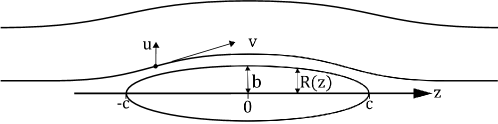
Figure 1: Velocity distribution of the fluid around a slender body. The streamline at which the velocity is indicated is supposed to be very close to the body. The transverse component $u$ of velocity is related to the total speed by the slope $R^{\prime}\left(z\right)$ of the body cross-section at the corresponding value of the coordinate $z$.

The sloped surface of the body accelerates the fluid in the transverse direction. Far from the body, the fluid travels also longitudinally and returns towards the $z$-axis in the downstream half of the body. In the rest frame of the fluid far from the body, the streamlines form a dipole-like pattern. Since the velocity far from the body is insensitive to the slenderness $\epsilon$, the far-field contribution of the fluid is neglected to uncover the leading logarithmic dependence of added mass on $\epsilon$.

In the slender-body approximation, motion in each plane $z=\text{ constant}$ is treated independently from other planes. This approximation originates with the 1924 work on Zeppelin airships.(munk:1924aa, ) The transverse velocity at any $r$ is thus related to its value at the boundary $R\left(z\right)$ by the continuity equation $2\pi ru\left(r,z\right)=2\pi R\left(z\right)u\left(R\left(z\right),z\right)$,

$$u\left(r,z\right)=\frac{R\left(z\right)u\left(R\left(z\right),z\right)}{r}.$$ (3)

The value at the boundary follows from the slope of the surface (see Fig. 1). Within the slender-body approximation, the angle between the velocity of the fluid $\bm{v}$ and the axis of the body is small and its sine and tangent are approximately equal, thus

$$u\left(R\left(z\right),z\right)=R^{\prime}\left(z\right)v,$$ (4)

so that finally

$$u\left(r,z\right)=\frac{R\left(z\right)R^{\prime}\left(z\right)}{r}v.$$ (5)

This is sufficient to determine the fluid’s kinetic energy $T$,

$$T=\frac{\rho}{2}\int_{\text{fluid}}\mbox{d}^{3}ru^{2}\left(r,z\right)=\pi\rho v^{2}\int_{-c}^{c}\left(RR^{\prime}\right)^{2}\mbox{d}z\int_{R\left(z\right)}^{\infty}\frac{\mbox{d}r}{r}.$$ (6)

The divergence of the $r$-integration at large distances is an artifact of the approximation that the motion in each plane $z=\text{constant}$ is independent of the motion in other planes. In fact, of course, far from the axis there is some longitudinal motion of the fluid and the radial velocity decreases faster than $1/r$. This happens at distances of the order of the length of the moving body.

However, for the purpose of determining the coefficient of the leading logarithm (of the slenderness parameter), that large-distance behavior need not be known. It is sufficient to know the logarithmic contribution at the lower limit. We replace the upper limit of the $r$-integration in eq. (6) by a cutoff $\Lambda$ of the order of the length of the body because the velocity field outside of this falls off faster than $1/r$, and so does not contribute to the logarithmic singularity in $\epsilon$.

Eq. (6) is valid for any axisymmetric slender body. For an ellipsoid it gives

$$R\left(z\right) =b\sqrt{1-\left(\frac{z}{c}\right)^{2}}$$ (7)

$$T \overset{\epsilon\to 0}{\sim}\pi\rho v^{2}\int_{-c}^{c}\left(RR^{\prime}\right)^{2}\ln\frac{\Lambda}{R\left(z\right)}\mbox{d}z$$ (8)

$$=\frac{2\pi}{3}\rho v^{2}cb^{2}\epsilon^{2}\left(\ln\frac{1}{\epsilon}+\mathcal{O}\left(1\right)\right).$$ (9)

The volume of the ellipsoid being $\frac{4}{3}\pi cb^{2}$, within logarithmic accuracy this result becomes

$$T\sim\frac{m_{f}v^{2}}{2}\epsilon^{2}\ln\frac{1}{\epsilon},$$ (10)

where $m_{f}$ is the mass of the fluid displaced by the ellipsoid. The total kinetic energy of the body and the fluid is

$$T=\left(m_{b}+C_{{\scriptscriptstyle M}}m_{f}\right)\frac{v^{2}}{2}$$ (11)

where $m_{b}$ is the mass of the body. Comparison of Eqs. (10) and (11) gives the added mass coefficient (cf. Eq. 1),

$$C_{{\scriptscriptstyle M}}\overset{\epsilon\to 0}{\sim}\epsilon^{2}\ln\frac{1}{\epsilon}.$$ (12)

For $\epsilon\simeq 0.3$, this gives $C_{{\scriptscriptstyle M}}\simeq 0.1$. A body of such shape could reach an acceleration of up to about $\frac{g}{C_{{\scriptscriptstyle M}}}\simeq 10g$. This leading order behaviour of the added mass coefficient is consistent with both the analytic solution in Appendix B and earlier slender body studies.(Handlesman, ) The following section describes experimental evidence of an acceleration exceeding $6g$.

III Experiment

III.1 Setup

The experimental setup is shown in Fig. 2. A spindle-shaped piece of styrofoam approximates an ellipsoid. Thin (0.005 inch or about 0.1 mm diameter) copper wire is attached to the bottom end of the spindle, which is completely submerged in a large cylindrical tank of water. The wire passes through a light plastic pulley at the bottom of the tank, and its end is held above the water surface.

A white mark on the wire facilitates tracking of the wire’s motion once it is released and pulled by the accelerating spindle. The section of the wire containing the white mark passes through a glass tube that guides the wire along a millimeter precision ruler in front of a high-speed camera. The field of view of the camera includes about 12 cm of the distance the white mark travels. The advantage of this arrangement is that all photography and measurements are made above water.

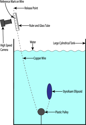
Figure 2: The experimental setup. A thin copper wire is attached to the bottom of the approximate ellipsoid (spindle) made of styrofoam. The wire is fed through a pulley, then through a glass tube placed against a ruler. The motion of a reference mark on the wire is registered with a high speed camera.

A perfect material for producing the spindle is the so-called extruded polystyrene foam. Produced by Dow Chemical Company and marketed as Styrofoam Cladmate CM20, it is a readily available and inexpensive construction insulation material, able to withstand compression. It is easily cut with hot wire and finely shaped with abrasive paper on a stationary belt sander. Its density is only about 1/40 of water and its moisture-resistance prevents water from penetrating, protecting its low inertia. The spindle is 28 cm long and has about 6 cm mean diameter in its thickest cross section. A spindle volume of 0.44 liter is determined from its mass, 10.8 grams. The spindle shape differs from an ellipsoid by protruding tips. Its slenderness parameter is thus estimated by $\epsilon\simeq 0.3$, assuming the length of an equivalent ellipsoid to be about 20 cm.

In order to attach the copper wire to the spindle, the wire is inserted in a small incision of about one inch depth and secured with cyanoacrylate Super Glue. The thin copper wire is prone to twisting, breaking, and falling off the pulley, and takes some practice to work with. However, it has a much higher Young modulus than a fishing line that was initially employed. The wire tension due to the buoyancy of the spindle is about 4 N, at which the 1.5-meter wire stretches less than a centimeter, much less than the distance over which the motion is observed. This removes the only systematic uncertainty that was identified to possibly increase the acceleration of the wire mark compared to the actual acceleration of the spindle.

All other effects: drag, friction, finite size of the tank, mass of the wire and the moment of inertia of the pulley act to decrease the observed acceleration. Since the goal was to prove that the acceleration can exceed $2g$ rather than to precisely measure it, these systematic effects are unimportant for our purposes.

The high-speed camera is NAC Image Technology’s HotShot HS1280cc, set to 700 frames per second. At this speed, very strong light is required, so the marked part of the wire is illuminated with a Lowel Pro-Light with a 250 W halogen bulb by Osram. To eliminate ambient light, a sheet of dark construction paper is used as a backdrop.

III.2 Results

The pictures of the wire motion are processed with the free image analysis software Tracker.(TRACKER, ) The raw displacement data from an example run are presented in panel (a) of Fig. 3. The displacement curve has an overall upward curvature indicative of acceleration. A quadratic fit to these data, $d\left(t\right)=\frac{at^{2}}{2}+v_{0}t+d$, is plotted with a solid line.

Note that the 0 second mark on the time axis does not necessarily coincide with the release time, which is not registered. If the first 29 ms are excluded, the fit results in the acceleration of $63.7\text{ $\frac{\text{m}}{\text{s}^{2}}$}$. Assuming gravitational acceleration in Edmonton, Alberta, to be $g=9.838\text{ $\frac{\text{m}}{\text{s}^{2}}$}$, this translates into about $6.48g$. A fit starting at 35 ms gives instead $62.1\text{ $\frac{\text{m}}{\text{s}^{2}}$\;}$ or $6.31g$.

An alternative analysis is based on the velocity of the spindle, determined from the displacement data, plotted in Fig. 3. Panel (b) shows the velocity determined from neighboring data points, based on the smooth central difference formula $v_{i}=\frac{d_{i+1}-d_{i-1}}{2\Delta t}$.

The plot clearly illustrates linear velocity growth starting around 35 ms. A linear fit to the region between 35 and 75 ms is sloped at about $6.33g$.

Below 30 ms, the displacement and the velocity data show a feature that may have resulted from the crude release of the wire (by hand) and possibly from the rapid initial contraction of the wire. This region is excluded from the analysis.

The final value of the spindle acceleration in the 35-75 ms window is $6.3\left(2\right)g$, where the conservative error estimate is based on the sensitivity to the starting point of the fit.

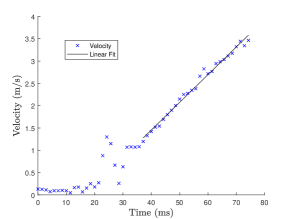
(a)                                                                         (b)

Figure 3: Panel (a) shows the spindle displacement as a function of time (ms) along with a quadratic fit made directly to the raw displacement data. Panel (b) shows the velocity of the spindle, as a function of time (ms), and a linear fit during the last 40 ms.

IV Discussion and Summary

The value of the spindle acceleration, $6.3\left(2\right)g$, is in reasonable agreement with the rough theoretical prediction for maximum acceleration of about $10g$ made in Section II. That estimate ignored all dissipative effects, the inertia of the pulley, and even the weight of the spindle and of the wire. It was based only on the added mass, which is therefore found to crucially influence the motion of a body immersed in a fluid. If the added mass were ignored, the buoyancy force of 4 N would have accelerated a body of mass $10.8$ gram at almost $40g$.

The experiment described here clearly shows that the common textbook neglect of the added mass is unrealistic and misleading, even for a slender body for which the added mass is relatively small. On the other hand, the experiment shows that the buoyancy can accelerate a body in fluid by significantly more than $2g$.

The theoretical value of acceleration may be refined by taking into account the finite mass of the styrofoam body. Then, Newton’s Second Law gives the acceleration

$$a=\frac{m_{b}-m_{f}}{m_{b}+C_{{\scriptscriptstyle M}}m_{f}}g,$$ (13)

where $m_{b}$ is the measured ellipsoid mass of 10.8 grams, $m_{f}$ is the mass of the displaced $0.44$ liter of water, and $C_{{\scriptscriptstyle M}}\simeq 0.1$ is the added mass coefficient obtained in the slender body approximation. Including the body mass suppresses the predicted acceleration to $7.3g$, in better agreement with the measured value $6.3\left(2\right)g$.

A full analytic solution to the added mass of the prolate spheroid, see Appendix B, agrees well with the simple expression derived in Section II even for $\epsilon\simeq 0.3$. The simple derivation alleviates the complexity of the complete solution in Appendix B without sacrificing significant accuracy as long as $\epsilon$ is fairly small.

The full analytic expression for the added mass coefficient gives rise to a theoretical acceleration of $8.3g$, further from the experimentally measured value than the leading slender body approximation. Higher order terms in the slenderness parameter reduce the added mass and thus increase the predicted acceleration.

The experiment described here can be relatively easily reproduced in class or during a field trip. It can also be extended: by making more marks on the wire, separated by less than the field of view of the camera, the motion can be tracked over a longer range. The acceleration should decrease exponentially due to drag. Such an observation could be used to determine the drag coefficient.(pantaleone:2011aa, ) Also the maximum height reached by the body after jumping above the water surface can be measured and compared with a prediction based on the observed terminal velocity. Another related experiment could involve an inverted pendulum attached at the bottom of the tank and fully submerged.

An expensive high-speed camera is not necessary for an interesting experiment. Modern cell phones reach 120 and even 240 frames per second, a rate at which about 10 data points would have been obtained in the window 35-75 ms analyzed in this paper. A feature of the setup described here is that all measurements are done above water, so the experiment can be carried out in a swimming pool or in a lake.

Despite its simplicity, this experiment introduces students to the advanced topic of mass renormalization. It also provides an opportunity to introduce elementary notions of hydrodynamics. Both limiting cases: of a sphere (slenderness parameter $\epsilon$ equal 1) and of a slender body ($\epsilon\ll 1$) can be treated with simple mathematical tools. In the case of the sphere, the calculation is analogous to the electrostatic problem of a conducting sphere inserted into a uniform electric field. Solving both problems in parallel illustrates how both Dirichlet and Neumann boundary conditions are used with the Laplace equation.

The slender body case described in Section II is related to the idea of a singular perturbation: the added-mass coefficient is not analytic in the limit of $\epsilon\to 0$ and contains a logarithm. This is one of the simplest physics problems that exhibits such a feature and can be used as a starting point of a deeper mathematical discussion.(bender1999methods, )

Appendix A Added mass of a sphere

In this paper we assume an ideal fluid, neglecting its viscosity and compressibility. The viscosity could play a role only in the very first moments of the motion; however, the magnitude of the viscous force is negligible in comparison with buoyancy when the velocity is close to zero.

Compressibility is negligible because the velocity is much smaller than the speed of sound throughout the observed motion.

The fluid pattern is assumed to be laminar in the determination of the added mass coefficient. This assumption is justified at the beginning of the motion when the velocity is very small. This is sufficient to predict the initial acceleration. The Reynolds number ${vR\over\nu}$ (with $v$ denoting the velocity of the body, $R$ its characteristic size, and $\nu\simeq 10^{-6}\,\text{m}^{2}/\text{s}$ the kinematic viscosity of water) is estimated to reach $10^{4}$ around the first centimeter of motion. In future studies it may be interesting to add dye to water to probe for the onset of turbulence.

A.1 Velocity potential

Kinetic energy of a fluid disturbed by a moving sphere is computed here, to explain the method.(Milne-Thomson-Hydr, ) The flow being irrotational, the fluid velocity is a gradient of a scalar function, the velocity potential, $\bm{v}=\bm{\nabla}\phi\left(\bm{r}\right)$. For an incompressible flow, the divergence of the velocity vanishes and $\phi$ satisfies the Laplace equation $\nabla^{2}\phi=0$. Spherical coordinates are employed, with the origin at the center of the sphere. Because of axial symmetry, $\phi$ is independent of the azimuth angle $\varphi$ and depends only on $r$ and $\theta$. Thus

$$r\partial_{r}^{2}\left(r\phi\right)+\partial_{\cos\theta}\left(\sin\theta\partial_{\cos\theta}\phi\right)=0.$$ (14)

In the rest frame of the fluid far from the sphere, the sphere is moving with speed $v$ along the $z$-axis. Denote the outward-drawn normal to the sphere surface by $\hat{n}$. The projection of the velocity $v\hat{z}$ of a surface element on that normal is $vn_{z}$ where $n_{z}=\hat{n}\cdot\hat{z}$. The kinematic boundary condition for the fluid velocity on the sphere surface $\left(r=c\right)$ is $\bm{v}\cdot\hat{n}=vn_{z}$ (the fluid is moving in the direction perpendicular to the surface with the same speed as the surface itself is moving in that direction). Thus the directional derivative of the velocity potential along the normal is

$$\frac{\partial\phi}{\partial n}=vn_{z}.$$ (15)

Since $n_{z}$ is the projection of the normal on the $z$-axis, $n_{z}\mbox{d}n=\mbox{d}z$. Thus $\phi_{s}\left(r,\theta\right)=vz$ satisfies the boundary condition (15) as well as the Laplace equation. This simple dependence only on $z$ is a general result, valid not only for the sphere; it will be used also for the ellipsoid.

However, $\phi_{s}$ does not satisfy the correct boundary condition at infinity, where the potential should be constant to give zero velocity. A suppression factor $f\left(r\right)$ is needed, independent of the direction. In order to find it, substitute into (14)

$$\phi\left(r,\theta\right)=v\phi_{s}\left(r,\theta\right)f\left(r\right),$$ (16)

Since $\phi_{s}\left(r,\theta\right)=vz=vr\cos\theta$ satisfies the Laplace equation, Eq. (14) becomes an ordinary differential equation for the factor $f\left(r\right)$, in which only its derivatives appear,

$$rf^{\prime\prime}\left(r\right)+4f^{\prime}\left(r\right)=0\implies f^{\prime}\left(r\right)=\frac{c_{1}}{r^{4}}\implies f\left(r\right)=\frac{c_{2}}{r^{3}}+c_{3},$$ (17)

where $c_{3}$ must vanish for proper behavior at $r\to\infty$. The complete velocity potential is

$$\phi\left(r,\theta\right)=vr\cos\theta f\left(r\right)=v\frac{c_{2}}{r^{2}}\cos\theta.$$ (18)

and the overall normalization $c_{2}=-\frac{c^{3}}{2}$ is fixed by the boundary condition Eq. (15) imposed on the surface of the sphere $r=c$,

$$\phi\left(r,\theta\right)=-v\frac{c^{3}}{2r^{2}}\cos\theta.$$ (19)

A.2 Kinetic energy of the fluid

In order to find the added-mass coefficient for the sphere, compute the kinetic energy of the fluid; Green’s theorem converts the integral over the volume of the fluid into one over its boundary: only the surface of the sphere contributes,

$$T =\frac{\rho}{2}\int\left(\bm{\nabla}\phi\left(\bm{r}\right)\right)^{2}\mbox{d}^{3}r=-\frac{\rho}{2}\int\phi\left(r=c,\theta\right)\bm{\nabla}\phi\cdot\mbox{d}^{2}\bm{S}=\frac{\rho}{4}v^{2}\underbrace{\int c\cos\theta\mbox{d}^{2}S}_{V}=\frac{1}{2}\cdot\frac{m_{f}v^{2}}{2},$$ (20)

where $m_{f}=V\rho$ is, as before, the mass of the displaced fluid and $V$ is the volume of the sphere.(Milne-Thomson-Hydr, ) In conclusion, the added-mass coefficient is $\frac{1}{2}$ for a sphere, in agreement with Ref. pantaleone:2011aa, .

Appendix B Added mass of a spheroid

B.1 Prolate spheroidal coordinates

Consider a prolate ellipsoid of revolution (a spheroid), with its long axis on the $z$-axis, and velocity $\bm{v}$ along $z$. Prolate spheroidal coordinates $\sigma,\tau,\varphi$ are convenient for finding the velocity potential of the disturbed fluid. They are related to Cartesian coordinates by

$$x =\sqrt{\left(\sigma^{2}-1\right)\left(1-\tau^{2}\right)}\cos\varphi$$ (21)

$$y =\sqrt{\left(\sigma^{2}-1\right)\left(1-\tau^{2}\right)}\sin\varphi$$ (22)

$$z =\sigma\tau.$$ (23)

Surfaces of constant $\sigma$ are spheroids symmetric around the $z$-axis. $\varphi$ is the usual azimuth angle; surfaces of constant $\varphi$ are planes containing the $z$-axis. Finally, $\tau$ parametrizes a family of two-sheet hyperboloids that intersect the spheroids and the constant-$\varphi$ planes at right angles. In a limit in which the spheroids become spheres, these hyperboloids become cones parametrized by a polar angle; in that sense $\tau$ replaces the $\cos\theta$ of spherical coordinates.

An element of distance squared is expressed as

$$\left(\mbox{d}s\right)^{2}=h_{\sigma}^{2}\left(\mbox{d}\sigma\right)^{2}+h_{\tau}^{2}\left(\mbox{d}\tau\right)^{2}+h_{\varphi}^{2}\left(\mbox{d}\varphi\right)^{2}$$ (24)

with

$$h_{\sigma}=\sqrt{\frac{\sigma^{2}-\tau^{2}}{\sigma^{2}-1}},\quad h_{\tau}=\sqrt{\frac{\sigma^{2}-\tau^{2}}{1-\tau^{2}}},\quad h_{\varphi}=\sqrt{\left(\sigma^{2}-1\right)\left(1-\tau^{2}\right)}.$$ (25)

B.2 Velocity potential

For an axially-symmetric problem, the velocity potential $\phi\left(\sigma,\tau\right)$ is independent of $\varphi$ and its Laplace equation becomes

$$\partial_{\sigma}\left[\left(\sigma^{2}-1\right)\partial_{\sigma}\phi\right]+\partial_{\tau}\left[\left(1-\tau^{2}\right)\partial_{\tau}\phi\right]=0.$$ (26)

On the surface of a spheroid with the ratio of short-to-long axes $\epsilon=\frac{b}{c}$, the coordinate $\sigma$ is constant,

$$\sigma=\sigma_{0}=\frac{1}{\sqrt{1-\epsilon^{2}}}.$$ (27)

The boundary condition (15) on the spheroid surface can be written as

$$\frac{\partial\phi}{\partial n}=vn_{z}\implies\frac{1}{h_{\sigma}}\frac{\partial\phi}{\partial\sigma}=v\cos\theta_{z}=\frac{v}{h_{\sigma}}\frac{\partial z}{\partial\sigma}\implies\frac{\partial\phi}{\partial\sigma}=v\frac{\partial z}{\partial\sigma}.$$ (28)

This condition is again satisfied by $\phi_{s}=vz=v\sigma\tau$ on the spheroid. All that is needed to complete the solution $\phi\left(\sigma,\tau\right)$ is the suppression factor $f\left(\sigma\right)$. Just like in Appendix A, the substitution $\phi=\phi_{s}f$ converts the Laplace equation (26) into a first order ODE for $f^{\prime}\left(\sigma\right)$,

$$\left(\sigma^{2}-1\right)\sigma f^{\prime\prime}\left(\sigma\right)+2\left(2\sigma^{2}-1\right)f^{\prime}\left(\sigma\right)=0.$$ (29)

Two integrations, with the condition of vanishing $f\left(\sigma\to\infty\right)$, give

$$f\left(\sigma\right)=C\left(\frac{1}{2}\ln\frac{\sigma+1}{\sigma-1}-\frac{1}{\sigma}\right).$$ (30)

Far from the origin, this is indeed a suppression factor, behaving like $f\left(\sigma\to\infty\right)\sim\frac{C}{3\sigma^{3}}$, like the analogous factor in spherical coordinates, eq. (17). In order to determine $C$, consider again the boundary condition on the spheroid,

$$\partial_{\sigma}\left[v\sigma\tau f\left(\sigma\right)\right]=v\frac{\partial z}{\partial\sigma}=v\tau,\qquad\left(\sigma=\sigma_{s}\right)$$ (31)

from which follows

$$\frac{1}{C}=f\left(\sigma_{0}\right)+\sigma_{0}f^{\prime}\left(\sigma_{0}\right)=\frac{1}{2}\ln\frac{\sigma_{0}+1}{\sigma_{0}-1}+\frac{\sigma_{0}}{1-\sigma_{0}^{2}},$$ (32)

and the complete potential reads

$$\phi\left(\sigma,\tau\right)=v\sigma\tau\frac{\frac{1}{2}\ln\frac{\sigma+1}{\sigma-1}-\frac{1}{\sigma}}{\frac{1}{2}\ln\frac{\sigma_{0}+1}{\sigma_{0}-1}+\frac{\sigma_{0}}{1-\sigma_{0}^{2}}}.$$ (33)

B.3 Added-mass coefficient for a spheroid

It is convenient to write the potential on the sphere as $\phi\left(\sigma_{0},\tau\right)=vzF$, where $F=1+\frac{2}{\sigma_{0}\left(\sigma_{0}^{2}-1\right)\ln\frac{\sigma_{0}+1}{\sigma_{0}-1}-2\sigma_{0}^{2}}$. In analogy with Appendix A.2, the integration in the kinetic energy expression gives the volume of the spheroid, and

$$T =-F\frac{m_{f}v^{2}}{2}.$$ (34)

Thus the added-mass coefficient is just $C_{{\scriptscriptstyle M}}=-F$. In terms of the slenderness parameter $\epsilon$, using Eq. (27),

$$C_{{\scriptscriptstyle M}}=\frac{1-\epsilon^{2}}{1-\frac{\epsilon^{2}}{\sqrt{1-\epsilon^{2}}}\ln\frac{1+\sqrt{1-\epsilon^{2}}}{\epsilon}}-1.$$ (35)

This general result has correct limiting behaviors: For a sphere, $\epsilon=1$, it correctly reproduces $C_{{\scriptscriptstyle M}}\left(\epsilon=1\right)=\frac{1}{2}$, derived in Appendix A.2. For a slender spheroid, $\epsilon\to 0$,

$$C_{{\scriptscriptstyle M}}\left(\epsilon\to 0\right)\sim\epsilon^{2}\ln\frac{1}{\epsilon},$$ (36)

in agreement with the derivation of Section II.

References

- (1) Leonard Meirovitch, Fundamentals of Vibrations, Waveland Press, 2010.
- (2) H.D. Young, R.A. Freedman, and A.L. Ford, Sears’ and Zemansky’s University Physics, Pearson, 14 edition, 2014.
- (3) Thomas Smid, "Beyond Archimedes’ Principle of Buoyancy," <https://www.physicsmyths.org.uk/buoyancy.htm>.
- (4) George Green, Mathematical papers of the late George Green, Macmillan, London, 1871.
- (5) A. Connes and M. Marcolli, Noncommutative Geometry, Quantum Fields and Motives, American Mathematical Society.
- (6) J. Messer and J. Pantaleone, "The effective mass of a ball in the air," The Physics Teacher, 48:52–54, 2010.
- (7) J. Pantaleone and J. Messer, "The added mass of a spherical projectile," Am. J. Phys, 79(12):1202–1210, 2011.
- (8) Robert E. O’Malley, Historical Developments in Singular Perturbations, Springer International Publishing, 2014.
- (9) Max M. Munk, "The aerodynamic forces on airship hulls," Technical Report NACA-TR-184, National Advisory Committee for Aeronautics, Washington, DC, 1924.
- (10) R.A. Handlesman and J.B. Keller, "Axially symmetric potential flow around a slender body", J. Fluid Mech., 38(1):131–147, 1967.
- (11) Tracker: free video analysis and modeling tool for physics education, <https://physlets.org/tracker/>.
- (12) C.M. Bender and S.A. Orszag, Advanced Mathematical Methods for Scientists and Engineers I: Asymptotic Methods and Perturbation Theory, Springer, New York, 1999.
- (13) L.M. Milne-Thomson, Theoretical Hydrodynamics, Macmillan, London, 4th edition, 1962.