Deep Representation Learning for Clustering of Health Tweets

Abstract

Twitter has been a prominent social media platform for mining population-level health data and accurate clustering of health-related tweets into topics is important for extracting relevant health insights. In this work, we propose deep convolutional autoencoders for learning compact representations of health-related tweets, further to be employed in clustering. We compare our method to several conventional tweet representation methods including bag-of-words, term frequency-inverse document frequency, Latent Dirichlet Allocation and Non-negative Matrix Factorization with 3 different clustering algorithms. Our results show that the clustering performance using proposed representation learning scheme significantly outperforms that of conventional methods for all experiments of different number of clusters. In addition, we propose a constraint on the learned representations during the neural network training in order to further enhance the clustering performance. All in all, this study introduces utilization of deep neural network-based architectures, i.e., deep convolutional autoencoders, for learning informative representations of health-related tweets.

I Introduction

Social media plays an important role in health informatics and Twitter has been one of the most influential social media channel for mining population-level health insights [1, 2, 3]. These insights range from forecasting of influenza epidemics [4] to predicting adverse drug reactions [5]. A notable challenge due to the short length of Twitter messages is categorization of tweets into topics in a supervised manner, i.e., topic classification, as well as in an unsupervised manner, i.e., clustering.

Classification of tweets into topics has been studied extensively [6, 7, 8]. Even though text classification algorithms can reach significant accuracy levels, supervised machine learning approaches require annotated data, i.e, topic categories to learn from for classification. On the other hand, annotated data is not always available as the annotation process is burdensome and time-consuming. In addition, discussions in social media evolve rapidly with recent trends, rendering Twitter a dynamic environment with ever-changing topics. Therefore, unsupervised approaches are essential for mining health-related information from Twitter.

Proposed methods for clustering tweets employ conventional text clustering pipelines involving preprocessing applied to raw text strings, followed by feature extraction which is then followed by a clustering algorithm [9, 10, 11]. Performance of such approaches depend highly on feature extraction in which careful engineering and domain knowledge is required [12]. Recent advancements in machine learning research, i.e., deep neural networks, enable efficient representation learning from raw data in a hierarchical manner [13, 14]. Several natural language processing (NLP) tasks involving Twitter data have benefited from deep neural network-based approaches including sentiment classification of tweets [15], predicting potential suicide attempts from Twitter [16] and simulating epidemics from Twitter [17].

In this work, we propose deep convolutional autoencoders (CAEs) for obtaining efficient representations of health-related tweets in an unsupervised manner. We validate our approach on a publicly available dataset from Twitter by comparing the performance of our approach and conventional feature extraction methods on 3 different clustering algorithms. Furthermore, we propose a constraint on the learned representations during neural network training in order to further improve the clustering performance. We show that the proposed deep neural network-based representation learning method outperforms conventional methods in terms of clustering performance in experiments of varying number of clusters.

II Related Work

Devising efficient representations of tweets, i.e., features, for performing clustering has been studied extensively. Most frequently used features for representing the text in tweets as numerical vectors are bag-of-words (BoWs) and term frequency-inverse document frequency (tf-idf) features [18, 10, 11, 19, 20]. Both of these feature extraction methods are based on word occurrence counts and eventually, result in a sparse (most elements being zero) document-term matrix. Proposed algorithms for clustering tweets into topics include variants of hierarchical, density-based and centroid-based clustering methods; k-means algorithm being the most frequently used one [10, 20, 21].

Numerous works on topic modeling of tweets are available as well. Topic models are generative models, relying on the idea that a given tweet is a mixture of topics, where a topic is a probability distribution over words [22]. Even though the objective in topic modeling is slightly different than that of pure clustering, representing each tweet as a topic vector is essentially a way of dimensionality reduction or feature extraction and can further be followed by a clustering algorithm. Proposed topic modeling methods include conventional approaches or variants of them such as Latent Dirichlet Allocation (LDA) [23, 18, 10, 24, 25, 26, 27, 28, 20, 29, 30] and Non-negative Matrix Factorization (NMF) [31, 19]. Note that topic models such as LDA are based on the notion that words belonging to a topic are more likely to appear in the same document and do not assume a distance metric between discovered topics.

In contrary to abovementioned feature extraction methods which are not specific to representation of tweets but rather generic in natural language processing, various works propose custom feature extraction methods for certain health-related information retrieval tasks from Twitter. For instance, Lim et al. engineered sentiment analysis features to discover latent infectious diseases from Twitter [32]. In order to track public health condition trends from Twitter, specific features are proposed by Parker at al. employing Wikipedia article index, i.e., treating the retrieval of medically-related Wikipedia articles as an indicator of a health-related condition [33]. Custom user similarity features calculated from tweets were also proposed for building a framework for recommending health-related topics [28].

The idea of learning effective representations from raw data using neural networks has been employed in numerous machine learning domains such as computer vision and natural language processing [13, 14]. The concept relies on the hierarchical, layer-wise architecture of neural networks in which the raw input data is encoded into informative representations of lower dimensions (representations of higher dimensions are possible as well) in a highly non-linear fashion. Autoencoders, Denoising Autoencoders, Convolutional Autoencoders, Sparse Autoencoders, Stacked Autoencoders and combinations of these, e.g., Denoising Convolutional Autoencoders, are the most common deep neural network architectures specifically used for representation learning. In an autoencoder training, the network tries to reconstruct the input data at its output, which forces the model to capture the most salient features of the data at its intermediate layers. If the intermediate layers correspond to a lower dimensional latent space than the original input, such autoencoders are also known as undercomplete. Activations extracted from these layers can be considered as compact, non-linear representations of the input.

Another significant advancement in neural network-based representation learning in NLP tasks is word embeddings (also called distributed representation of words). By representing each word in a given vocabulary with a real-valued vector of a fixed dimension, word embeddings enable capturing of lexical, semantic or even syntactic similarities between words. Typically, these vector representations are learned from large corpora and can be used to enhance the performance of numerous NLP tasks such as document classification, question answering and machine translation. Most frequently used word embeddings are word2vec [34] and GloVe (Global Vectors for Word Representation) [35]. Both of these are extracted in an unsupervised manner and are based on the distributional hypothesis [36], i.e., the assumption that words that occur in the same contexts tend to have similar meanings. Both word2vec and GloVe treat a word as a smallest entity to train on. A shift in this paradigm was introduced by fastText [37], which treats each word as a bag of character n-grams. Consequently, fastText embeddings are shown to have better representations for rare words [37]. In addition, one can still construct a vector representation for an out-of-vocabulary word which is not possible with word2vec or GloVe embeddings [37]. Enhanced methods for deducting better word and/or sentence representations were recently introduced as well by Peters et al. with the name ELMo (Embeddings from Language Models) [38] and by Devlin et al. with the name BERT (Bidirectional Encoder Representations from Transformers) [39]. All of these word embedding models are trained on large corpora such as Wikipedia, in an unsupervised manner. For analyzing tweets, word2vec and GloVe word embeddings have been employed for topical clustering of tweets [40], topic modeling [41, 42] and extracting depression symptoms from tweets [21].

Metrics for evaluating the performance of clustering algorithms varies depending on whether the ground truth topic categories are available or not. If so, frequently used metrics are accuracy and normalized mutual information. In the case of absence of ground truth labels, one has to use internal clustering criterions such as Calinski-Harabasz (CH) score [43] and Davies-Bouldin index [44]. Arbelaitz et al. provides an extensive comparative study of cluster validity indices [45].

III Methods

III-A Dataset

For this study, a publicly available dataset is used [46]. The dataset consisting of tweets has been collected using Twitter API and was initially introduced by Karami et al. [47]. Earliest tweet dates back to 13 June 2011 where the latest one has a timestamp of 9 April 2015. The dataset consists of 63,326 tweets in English language, collected from Twitter channels of 16 major health news agencies. List of health news channels and the number of tweets in the dataset from each channel can be examined from Table I.

TABLE I: Number of tweets, total number of words, number of unique words and average number of words for tweets from 16 health-related twitter channels.

Twitter Channel	Number of Tweets	Number of Words	Number of Unique Words	Mean Word Count
BBC Health	3,929	22,543	4,334	5.7
CBC Health	3,741	34,144	6,529	9.1
CNN Health	4,061	45,369	6,568	11.2
Everyday Health	3,239	37,032	3,966	11.4
Fox News Health	2,000	18,134	4,315	9.1
Guardian Healthcare	2,997	42,481	4,139	14.2
Goodhealth	7,864	105,370	8,002	13.4
Kaiser Health	3,509	39,182	5,133	11.2
LA Times Health	4,171	50,715	7,648	12.2
MSN Health	3,199	26,252	4,275	8.2
NBC Health	4,215	35,909	5,910	8.5
NPR Health	4,837	43,427	7,303	9.0
NY Times Health	6,245	62,726	8,567	10.0
Reuters Health	4,719	44,210	6,482	9.4
US News Health	1,400	16,546	2,869	11.8
WSJ Health	3,200	40,317	6,792	12.6

The outlook of a typical tweet from the dataset can be examined from Figure 1. For every tweet, the raw data consists of the tweet text and in most cases followed by a url to the original news article of the particular news source. This url string, if available, is removed from each tweet as it does not possess any natural language information. As Twitter allows several ways for users to interact such as retweeting or mentioning, these actions appear in the raw text as well. For retweets, an indicator string of ”RT” appears as a prefix in the raw data and for user mentions, a string of form ”@username” appears in the raw data. These two tokens are removed as well. In addition, hashtags are converted to plain tokens by removal of the ”#” sign appearing before them (e.g. <#pregnancy> becomes <pregnancy>). Number of words, number of unique words and mean word counts for each Twitter channel can also be examined from Table I. Longest tweet consists of 27 words.

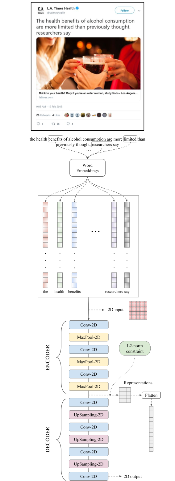
Figure 1: Proposed representation learning method depicting the overall flow starting from a tweet to the learned features, including the architecture of the convolutional autoencoder.

III-B Conventional Representations

For representing tweets, 5 conventional representation methods are proposed as baselines.

1. Word frequency features: For word occurrence-based representations of tweets, conventional tf-idf and BoWs are used to obtain the document-term matrix of $N\times P$ in which each row corresponds to a tweet and each column corresponds to a unique word/token, i.e., $N$ data points and $P$ features. As the document-term matrix obtained from tf-idf or BoWs features is extremely sparse and consequently redundant across many dimensions, dimensionality reduction and topic modeling to a lower dimensional latent space is performed by the methods below.

2. Principal Component Analysis (PCA): PCA is used to map the word frequency representations from the original feature space to a lower dimensional feature space by an orthogonal linear transformation in such a way that the first principal component has the highest possible variance and similarly, each succeeding component has the highest variance possible while being orthogonal to the preceding components. Our PCA implementation has a time complexity of $\mathcal{O}(NP^{2}+P^{3})$.

3. Truncated Singular Value Decomposition (t-SVD): Standard SVD and t-SVD are commonly employed dimensionality reduction techniques in which a matrix is reduced or approximated into a low-rank decomposition. Time complexity of SVD and t-SVD for $S$ components are $\mathcal{O}(min(NP^{2},N^{2}P))$ and $\mathcal{O}(N^{2}S)$, respectively (depending on the implementation). Contrary to PCA, t-SVD can be applied to sparse matrices efficiently as it does not require data normalization. When the data matrix is obtained by BoWs or tf-idf representations as in our case, the technique is also known as Latent Semantic Analysis.

4. LDA: Our LDA implementation employs online variational Bayes algorithm introduced by Hoffman et al. which uses stochastic optimization to maximize the objective function for the topic model [48].

5. NMF: As NMF finds two non-negative matrices whose product approximates the non-negative document-term matrix, it allows regularization. Our implementation did not employ any regularization and the divergence function is set to be squared error, i.e., Frobenius norm.

III-C Representation Learning

We propose 2D convolutional autoencoders for extracting compact representations of tweets from their raw form in a highly non-linear fashion. In order to turn a given tweet into a 2D structure to be fed into the CAE, we extract the word vectors of each word using word embedding models, i.e., for a given tweet, $t$, consisting of $W$ words, the 2D input is $I_{t}\in\R^{W\times D}$ where $D$ is the embedding vector dimension. We compare 4 different word embeddings namely word2vec, GloVe, fastText and BERT with embedding vector dimensions of 300, 300, 300 and 768, respectively. We set the maximum sequence length to 32, i.e., for tweets having less number of words, the input matrix is padded with zeros. As word2vec and GloVe embeddings can not handle out-of-vocabulary words, such cases are represented as a vector of zeros. The process of extracting word vector representations of a tweet to form the 2D input matrix can be examined from Figure 1.

The CAE architecture can be considered as consisting of 2 parts, ie., the encoder and the decoder. The encoder, $f_{enc}(\cdot)$, is the part of the network that compresses the input, $I$, into a latent space representation, $U$, and the decoder, $f_{dec}(\cdot)$ aims to reconstruct the input from the latent space representation (see equation 1). In essence,

$$U=f_{enc}(I)=f_{L}(f_{L-1}(...f_{1}(I)))$$ (1)

where $L$ is the number of layers in the encoder part of the CAE.

The encoder in the proposed architecture consists of three 2D convolutional layers with 64, 32 and 1 filters, respectively. The decoder follows the same symmetry with three convolutional layers with 1, 32 and 64 filters, respectively and an output convolutional layer of a single filter (see Figure 1). All convolutional layers have a kernel size of (3$\times$3) and an activation function of Rectified Linear Unit (ReLU) except the output layer which employs a linear activation function. Each convolutional layer in the encoder is followed by a 2D MaxPooling layer and similarly each convolutional layer in the decoder is followed by a 2D UpSampling layer, serving as an inverse operation (having the same parameters). The pooling sizes for pooling layers are (2$\times$5), (2$\times$5) and (2$\times$2), respectively for the architectures when word2vec, GloVe and fastText embeddings are employed. With this configuration, an input tweet of size $32\times 300$ (corresponding to maximum sequence length $\times$ embedding dimension, $D$) is downsampled to size of $4\times 6$ out of the encoder (bottleneck layer). As BERT word embeddings have word vectors of fixed size 768, the pooling layer sizes are chosen to be (2$\times$8), (2$\times$8) and (2$\times$2), respectively for that case. In summary, a representation of $4\times 6=24$ values is learned for each tweet through the encoder, e.g., for fastText embeddings the flow of dimensions after each encoder block is as such : $32\times 300\rightarrow 16\times 60\rightarrow 8\times 12\rightarrow 4\times 6$.

In numerous NLP tasks, an Embedding Layer is employed as the first layer of the neural network which can be initialized with the word embedding matrix in order to incorporate the embedding process into the architecture itself instead of manual extraction. In our case, this was not possible because of nonexistence of an inversed embedding layer in the decoder (as in the relationship between MaxPooling layers and UpSampling layers) as an embedding layer is not differentiable.

Training of autoencoders tries to minimize the reconstruction error/loss, i.e., the deviation of the reconstructed output from the input. $L_{2}$-loss or mean square error (MSE) is chosen to be the loss function. In autoencoders, minimizing the $L_{2}$-loss is equivalent to maximizing the mutual information between the reconstructed inputs and the original ones [49]. In addition, from a probabilistic point of view, minimizing the $L_{2}$-loss is the same as maximizing the probability of the parameters given the data, corresponding to a maximum likelihood estimator. The optimizer for the autoencoder training is chosen to be Adam due to its faster convergence abilities [50]. The learning rate for the optimizer is set to $10^{-5}$ and the batch size for the training is set to 32. Random split of 80% training-20% validation set is performed for monitoring convergence. Maximum number of training epochs is set to 50.

III-D $L_{2}$-norm Constrained Representation Learning

Certain constraints on neural network weights are commonly employed during training in order to reduce overfitting, also known as regularization. Such constraints include $L_{1}$ regularization, $L_{2}$ regularization, orthogonal regularization etc. Even though regularization is a common practice, standard training of neural networks do not inherently impose any constraints on the learned representations (activations), $U$, other than the ones compelled by the activation functions (e.g. ReLUs resulting in non-negative outputs). Recent advancements in computer vision research show that constraining the learned representations can enhance the effectiveness of representation learning, consequently increasing the clustering performance [51, 52].

$$\aligned&\text{minimize}L=1/_{N}\left\lVert I-f_{dec}(f_{enc}(I))\right\rVert^{2}_{2}\\ \text{subjectto}\left\lVert f_{enc}(I)\right\rVert^{2}_{2}=1$$ (2)

We propose an $L_{2}$ norm constraint on the learned representations out of the bottleneck layer, $U$. Essentially, this is a hard constraint introduced during neural network training that results in learned features with unit $L_{2}$ norm out of the bottleneck layer (see equation 2 where $N$ is the number of data points). Training a deep convolutional autoencoder with such a constraint is shown to be much more effective for image data than applying $L_{2}$ normalization on the learned representations after training [52]. To the best of our knowledge, this is the first study to incorporate $L_{2}$ norm constraint in a task involving text data.

III-E Evaluation

In order to fairly compare and evaluate the proposed methods in terms of effectiveness in representation of tweets, we fix the number of features to 24 for all methods and feed these representations as an input to 3 different clustering algorithms namely, k-means, Ward and spectral clustering with cluster numbers of 10, 20 and 50. Distance metric for k-means clustering is chosen to be euclidean and the linkage criteria for Ward clustering is chosen to be minimizing the sum of differences within all clusters, i.e., recursively merging pairs of clusters that minimally increases the within-cluster variance in a hierarchical manner. For spectral clustering, Gaussian kernel has been employed for constructing the affinity matrix. We also run experiments with tf-idf and BoWs representations without further dimensionality reduction as well as concatenation of all word embeddings into a long feature vector. For evaluation of clustering performance, we use Calinski-Harabasz score [43], also known as the variance ratio criterion. CH score is defined as the ratio between the within-cluster dispersion and the between-cluster dispersion. CH score has a range of $[0,+\infty]$ and a higher CH score corresponds to a better clustering. Computational complexity of calculating CH score is $\mathcal{O}(N)$.

For a given dataset $X$ consisting of $N$ data points, i.e., $X=\big{\{}x_{1},x_{2},...,x_{N}\big{\}}$ and a given set of disjoint clusters $C$ with $K$ clusters, i.e., $C=\big{\{}c_{1},c_{2},...,c_{K}\big{\}}$, Calinski-Harabasz score, $S_{CH}$, is defined as

$$S_{CH}=\frac{N-K}{K-1}\frac{\sum_{c_{k}\in C}{N_{k}\left\lVert\overline{c_{k}}-\overline{X}\right\rVert^{2}_{2}}}{\sum_{c_{k}\in C}{}\sum_{x_{i}\in c_{k}}{\left\lVert x_{i}-\overline{c_{k}}\right\rVert^{2}_{2}}}$$ (3)

where $N_{k}$ is the number of points belonging to the cluster $c_{k}$, $\overline{X}$ is the centroid of the entire dataset, $\frac{1}{N}\sum_{x_{i}\in X}{x_{i}}$ and $\overline{c_{k}}$ is the centroid of the cluster $c_{k}$, $\frac{1}{N_{k}}\sum_{x_{i}\in c_{k}}{x_{i}}$.

For visual validation, we plot and inspect the t-Distributed Stochastic Neighbor Embedding (t-SNE) [53] and Uniform Manifold Approximation and Projection (UMAP) [54] mappings of the learned representations as well. Implementation of this study is done in Python (version 3.6) using scikit-learn and TensorFlow libraries [55, 56] on a 64-bit Ubuntu 16.04 workstation with 128 GB RAM. Training of autoencoders are performed with a single NVIDIA Titan Xp GPU.

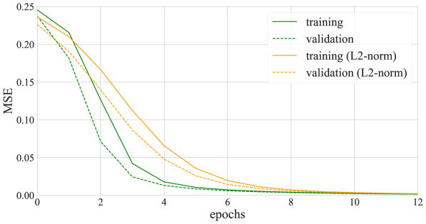
Figure 2: Learning curves depicting training and validation losses of CAE and $L_{2}$-norm constrained CAE architectures for fastText embeddings.

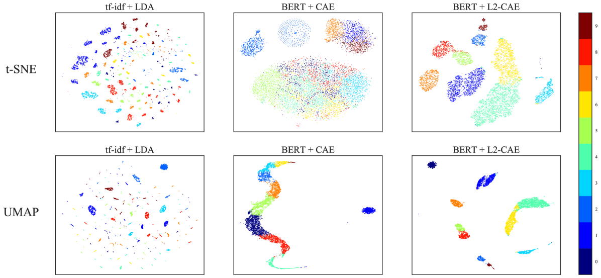
Figure 3: UMAP and t-SNE visualizations of representations extracted by LDA, CAE and $L_{2}$-norm constrained CAE (each having a length of 24) and coloring based on k-means clustering of the representations into 10 clusters.

IV Results

Performance of the representations tested on 3 different clustering algorithms, i.e., CH scores, for 3 different cluster numbers can be examined from Table II. $L_{2}$-norm constrained CAE is simply referred as $L_{2}$-CAE in Table II. Same table shows the number of features used for each method as well. Document-term matrix extracted by BoWs and tf-idf features result in a sparse matrix of $63,326\times 13,026$ with a sparsity of 0.9994733. Similarly, concatenation of word embeddings result in a high number of features with $32\times 300=9,600$ for word2vec, GloVe and fastText, $32\times 768=24,576$ for BERT embeddings. In summary, the proposed method of learning representations of tweets with CAEs outperform all of the conventional algorithms. When representations are compared with Hotelling’s $T^{2}$ test (multivariate version of $t$-test), every representation distribution learned by CAEs are shown to be statistically significantly different than every other conventional representation distribution with $p<0.001$. In addition, introducing the $L_{2}$-norm constraint on the learned representations during training enhances the clustering performance further (again $p<0.001$ when comparing for example fastText+CAE vs. fastText+$L_{2}$-CAE). An example learning curve for CAE and $L_{2}$-CAE with fastText embeddings as input can also be seen in Figure 2.

TABLE II: Calinski-Harabasz scores for several conventional methods and proposed cae-based methods for 3 different clustering algorithms and 3 different number of clusters.

		10 clusters			20 clusters			50 clusters
Tweet Representation	Features	k-means	Ward	spectral	k-means	Ward	spectral	k-means	Ward	spectral
tf-idf	13026	23	14	9	15	12	7	12	9	5
BoW	13026	23	25	9	18	19	7	15	13	5
word2vec (concatenated)	9600	174	152	110	78	61	64	41	33	21
GloVe (concatenated)	9600	157	131	119	97	63	71	43	37	27
fastText (concatenated)	9600	212	163	135	115	84	97	54	50	39
BERT (concatenated)	24576	206	171	138	123	85	94	57	42	41
tf-idf + PCA	24	443	333	320	421	316	309	421	396	395
BoW + PCA	24	679	411	679	543	412	498	507	489	495
tf-idf + t-SVD	24	419	294	284	437	326	337	404	384	394
BoW + t-SVD	24	633	385	630	579	427	510	495	480	493
tf-idf + LDA	24	684	497	627	621	486	620	638	433	614
BoW + LDA	24	408	280	403	355	260	359	284	214	271
tf-idf + NMF	24	444	406	434	413	452	449	521	527	594
BoW + NMF	24	512	477	636	491	460	563	591	556	600
word2vec + CAE	24	1851	1570	1726	1492	1357	1387	1317	1241	1040
GloVe + CAE	24	1953	1612	1696	1499	1302	1278	1367	1278	1102
fastText + CAE	24	3520	3173	3297	1914	1699	1772	1765	1567	1677
BERT + CAE	24	3467	3203	3288	2032	1768	1882	1834	1645	1711
word2vec + $L_{2}$-CAE	24	3060	2964	2998	2513	2424	2501	2284	2043	2193
GloVe + $L_{2}$-CAE	24	3100	2931	3017	2602	2499	2526	2280	2076	2200
fastText + $L_{2}$-CAE	24	6894	6884	6803	5839	5684	5743	4304	4187	4016
BERT + $L_{2}$-CAE	24	7703	7071	6972	5768	5606	4554	4172	4014	2559

Detailed inspection of tweets that are clustered into the same cluster as well as visual analysis of the formed clusters is also performed. Figure 3 shows the t-SNE and UMAP mappings (onto 2D plane) of the 10 clusters formed by k-means algorithm for LDA, CAE and $L_{2}$-CAE representations. Below are several examples of tweets sampled from one of the clusters formed by k-means in the 50 clusters case (fastText embeddings fed into $L_{2}$-CAE):

• <Suicide risk falls after talk therapy>

• <Air pollution may be tied to anxiety>

• <Stress, depression boost risks for heart patients>

• <Nearly 1 in 5 Americans who has been out of work for at least 1 year is clinically depressed.>

• <Study shows how exercise protects the brain against depression>

V Discussion

Overall, we show that deep convolutional autoencoder-based feature extraction, i.e., representation learning, from health related tweets significantly enhances the performance of clustering algorithms when compared to conventional text feature extraction and topic modeling methods (see Table II). This statement holds true for 3 different clustering algorithms (k-means, Ward, spectral) as well as for 3 different number of clusters. In addition, proposed constrained training ($L_{2}$-norm constraint) is shown to further improve the clustering performance in each experiment as well (see Table II). A Calinski-Harabasz score of 4,304 has been achieved with constrained representation learning by CAE for the experiment of 50 clusters formed by k-means clustering. The highest CH score achieved in the same experiment setting by conventional algorithms was 638 which was achieved by LDA applied of tf-idf features.

Visualizations of t-SNE and UMAP mappings in Figure 3 show that $L_{2}$-norm constrained training results in higher separability of clusters. The benefit of this constraint is especially significant in the performance of k-means clustering (see Table II). This phenomena is not unexpected as k-means clustering is based on $L_{2}$ distance as well. The difference in learning curves for regular and constrained CAE trainings is also expected. Constrained CAE training converges to local minimum slightly later than unconstrained CAE, i.e., training of $L_{2}$-CAE is slightly slower than that of CAE due to the introduced contraint (see Figure 2).

When it comes to comparison between word embeddings, fastText and BERT word vectors result in the highest CH scores whereas word2vec and GloVe embeddings result in significantly lower performance. This observation can be explained by the nature of word2vec and GloVe embeddings which can not handle out-of-vocabulary tokens. Numerous tweets include names of certain drugs which are more likely to be absent in the vocabulary of these models, consequently resulting in vectors of zeros as embeddings. However, fastText embeddings are based on character n-grams which enables handling of out-of-vocabulary tokens, e.g., fastText word vectors of the tokens <acetaminophen> and <paracetamol> are closer to each other simply due to shared character sequence, <acetam>, even if one of them is not in the vocabulary. Note that, <acetaminophen> and <paracetamol> are different names for the same drug.

Using tf-idf or BoWs features directly results in very poor performance. Similarly, concatenating word embeddings to create thousands of features results in significantly low performance compared to methods that reduce these features to 24. The main reason is that the bias-variance trade-off is dominated by the bias in high dimensional settings especially in Euclidean spaces [57]. Due to very high number of features (relative to the number of observations), the radius of a given region varies with respect to the $n$th root of its volume, whereas the number of data points in the region varies roughly linearly with the volume [57]. This phenomena is known as curse of dimensionality. As topic models such as LDA and NMF are designed to be used on documents that are sufficiently long to extract robust statistics from, extracted topic vectors fall short in performance as well when it comes to tweets due to short texts.

The main limitation of this study is the absence of topic labels in the dataset. As a result, internal clustering measure of Calinski-Harabasz score was used for evaluating the performance of the formed clusters instead of accuracy or normalized mutual information. Even though CH score is shown to be able to capture clusters of different densities and presence of subclusters, it has difficulties capturing highly noisy data and skewed distributions [58]. In addition, used clustering algorithms, i.e., k-means, Ward and spectral clustering, are hard clustering algorithms which results in non-overlapping clusters. However, a given tweet can have several topical labels.

Future work includes representation learning of health-related tweets using deep neural network architectures that can inherently learn the sequential nature of the textual data such as recurrent neural networks, e.g., Long Short-Term Memory (LSTM), Gated Recurrent Unit (GRU) etc. Sequence-to-sequence autoencoders are main examples of such architectures and they have been shown to be effective in encoding paragraphs from Wikipedia and other corpora to lower dimensions [59]. Furthermore, encodings out of a bidirectional GRU will be tested for clustering performance, as such architectures have been employed to represent a given tweet in other studies [60, 61, 62].

VI Conclusion

In summary, we show that deep convolutional autoencoders can effectively learn compact representations of health-related tweets in an unsupervised manner. Conducted analysis show that the proposed representation learning scheme outperforms conventional feature extraction methods in three different clustering algorithms. In addition, we propose a constraint on the learned representation in order to further increase the clustering performance. Future work includes comparison of our model with recurrent neural architectures for clustering of health-related tweets. We believe this study serves as an advancement in the field of natural language processing for health informatics especially in clustering of short-text social media data.

References

- [1] K. Vance, W. Howe, and R. P. Dellavalle, “Social internet sites as a source of public health information,” Dermatologic clinics, vol. 27, no. 2, pp. 133–136, 2009.
- [2] M. J. Paul and M. Dredze, “You are what you tweet: Analyzing twitter for public health.” Icwsm, vol. 20, pp. 265–272, 2011.
- [3] “Twitter,” https://twitter.com/, accessed: 2018-10-12.
- [4] H. Achrekar, A. Gandhe, R. Lazarus, S.-H. Yu, and B. Liu, “Predicting flu trends using twitter data,” in Computer Communications Workshops (INFOCOM WKSHPS), 2011 IEEE Conference on. IEEE, 2011, pp. 702–707.
- [5] J. Bian, U. Topaloglu, and F. Yu, “Towards large-scale twitter mining for drug-related adverse events,” in Proceedings of the 2012 international workshop on Smart health and wellbeing. ACM, 2012, pp. 25–32.
- [6] B. Sriram, D. Fuhry, E. Demir, H. Ferhatosmanoglu, and M. Demirbas, “Short text classification in twitter to improve information filtering,” in Proceedings of the 33rd international ACM SIGIR conference on Research and development in information retrieval. ACM, 2010, pp. 841–842.
- [7] R. Batool, A. M. Khattak, J. Maqbool, and S. Lee, “Precise tweet classification and sentiment analysis,” in Computer and Information Science (ICIS), 2013 IEEE/ACIS 12th International Conference on. IEEE, 2013, pp. 461–466.
- [8] A. Theodotou and A. Stassopoulou, “A system for automatic classification of twitter messages into categories,” in International and Interdisciplinary Conference on Modeling and Using Context. Springer, 2015, pp. 532–537.
- [9] Y. Lu, P. Zhang, J. Liu, J. Li, and S. Deng, “Health-related hot topic detection in online communities using text clustering,” Plos one, vol. 8, no. 2, p. e56221, 2013.
- [10] K. D. Rosa, R. Shah, B. Lin, A. Gershman, and R. Frederking, “Topical clustering of tweets,” Proceedings of the ACM SIGIR: SWSM, 2011.
- [11] S. B. Kaleel and A. Abhari, “Cluster-discovery of twitter messages for event detection and trending,” Journal of Computational Science, vol. 6, pp. 47–57, 2015.
- [12] Y. LeCun, Y. Bengio, and G. Hinton, “Deep learning,” Nature, vol. 521, no. 7553, p. 436, 2015.
- [13] G. E. Hinton and R. R. Salakhutdinov, “Reducing the dimensionality of data with neural networks,” science, vol. 313, no. 5786, pp. 504–507, 2006.
- [14] Y. Bengio, A. Courville, and P. Vincent, “Representation learning: A review and new perspectives,” IEEE transactions on pattern analysis and machine intelligence, vol. 35, no. 8, pp. 1798–1828, 2013.
- [15] A. Severyn and A. Moschitti, “Unitn: Training deep convolutional neural network for twitter sentiment classification,” in Proceedings of the 9th international workshop on semantic evaluation (SemEval 2015), 2015, pp. 464–469.
- [16] A. Benton, M. Mitchell, and D. Hovy, “Multi-task learning for mental health using social media text,” arXiv preprint arXiv:1712.03538, 2017.
- [17] L. Zhao, J. Chen, F. Chen, W. Wang, C.-T. Lu, and N. Ramakrishnan, “Simnest: Social media nested epidemic simulation via online semi-supervised deep learning,” in Data Mining (ICDM), 2015 IEEE International Conference on. IEEE, 2015, pp. 639–648.
- [18] D. Ramage, S. T. Dumais, and D. J. Liebling, “Characterizing microblogs with topic models.” ICWSM, vol. 10, no. 1, p. 16, 2010.
- [19] W. Yang and L. Mu, “Gis analysis of depression among twitter users,” Applied Geography, vol. 60, pp. 217–223, 2015.
- [20] S. L. Lo, R. Chiong, and D. Cornforth, “An unsupervised multilingual approach for online social media topic identification,” Expert Systems with Applications, vol. 81, pp. 282–298, 2017.
- [21] L. Ma, Z. Wang, and Y. Zhang, “Extracting depression symptoms from social networks and web blogs via text mining,” in International Symposium on Bioinformatics Research and Applications. Springer, 2017, pp. 325–330.
- [22] M. Steyvers and T. Griffiths, “Probabilistic topic models,” Handbook of latent semantic analysis, vol. 427, no. 7, pp. 424–440, 2007.
- [23] D. M. Blei, A. Y. Ng, and M. I. Jordan, “Latent dirichlet allocation,” Journal of machine Learning research, vol. 3, no. Jan, pp. 993–1022, 2003.
- [24] K. W. Prier, M. S. Smith, C. Giraud-Carrier, and C. L. Hanson, “Identifying health-related topics on twitter,” in International conference on social computing, behavioral-cultural modeling, and prediction. Springer, 2011, pp. 18–25.
- [25] L. Hannachi, O. Asfari, N. Benblidia, F. Bentayeb, N. Kabachi, and O. Boussaid, “Community extraction based on topic-driven-model for clustering users tweets,” in International Conference on Advanced Data Mining and Applications. Springer, 2012, pp. 39–51.
- [26] M.-C. Yang and H.-C. Rim, “Identifying interesting twitter contents using topical analysis,” Expert Systems with Applications, vol. 41, no. 9, pp. 4330–4336, 2014.
- [27] M. J. Paul and M. Dredze, “Discovering health topics in social media using topic models,” PloS one, vol. 9, no. 8, p. e103408, 2014.
- [28] V. V. Kaveri and V. Maheswari, “A framework for recommending health-related topics based on topic modeling in conversational data (twitter),” Cluster Computing, pp. 1–6, 2017.
- [29] A. Karami, A. A. Dahl, G. Turner-McGrievy, H. Kharrazi, and G. Shaw, “Characterizing diabetes, diet, exercise, and obesity comments on twitter,” International Journal of Information Management, vol. 38, no. 1, pp. 1–6, 2018.
- [30] A. Karami, F. Webb, and V. L. Kitzie, “Characterizing transgender health issues in twitter,” arXiv preprint arXiv:1808.06022, 2018.
- [31] X. Yan, J. Guo, S. Liu, X.-q. Cheng, and Y. Wang, “Clustering short text using ncut-weighted non-negative matrix factorization,” in Proceedings of the 21st ACM international conference on Information and knowledge management. ACM, 2012, pp. 2259–2262.
- [32] S. Lim, C. S. Tucker, and S. Kumara, “An unsupervised machine learning model for discovering latent infectious diseases using social media data,” Journal of biomedical informatics, vol. 66, pp. 82–94, 2017.
- [33] J. Parker, Y. Wei, A. Yates, O. Frieder, and N. Goharian, “A framework for detecting public health trends with twitter,” in Proceedings of the 2013 IEEE/ACM International Conference on Advances in Social Networks Analysis and Mining. ACM, 2013, pp. 556–563.
- [34] T. Mikolov, K. Chen, G. Corrado, and J. Dean, “Efficient estimation of word representations in vector space,” arXiv preprint arXiv:1301.3781, 2013.
- [35] J. Pennington, R. Socher, and C. Manning, “Glove: Global vectors for word representation,” in Proceedings of the 2014 conference on empirical methods in natural language processing (EMNLP), 2014, pp. 1532–1543.
- [36] Z. S. Harris, “Distributional structure,” Word, vol. 10, no. 2-3, pp. 146–162, 1954.
- [37] P. Bojanowski, E. Grave, A. Joulin, and T. Mikolov, “Enriching word vectors with subword information,” arXiv preprint arXiv:1607.04606, 2016.
- [38] M. E. Peters, M. Neumann, M. Iyyer, M. Gardner, C. Clark, K. Lee, and L. Zettlemoyer, “Deep contextualized word representations,” arXiv preprint arXiv:1802.05365, 2018.
- [39] J. Devlin, M.-W. Chang, K. Lee, and K. Toutanova, “Bert: Pre-training of deep bidirectional transformers for language understanding,” arXiv preprint arXiv:1810.04805, 2018.
- [40] X. Dai, M. Bikdash, and B. Meyer, “From social media to public health surveillance: Word embedding based clustering method for twitter classification,” in SoutheastCon, 2017. IEEE, 2017, pp. 1–7.
- [41] V. K. R. Sridhar, “Unsupervised topic modeling for short texts using distributed representations of words,” in Proceedings of the 1st workshop on vector space modeling for natural language processing, 2015, pp. 192–200.
- [42] D. Q. Nguyen, R. Billingsley, L. Du, and M. Johnson, “Improving topic models with latent feature word representations,” arXiv preprint arXiv:1810.06306, 2018.
- [43] T. Caliński and J. Harabasz, “A dendrite method for cluster analysis,” Communications in Statistics-theory and Methods, vol. 3, no. 1, pp. 1–27, 1974.
- [44] D. L. Davies and D. W. Bouldin, “A cluster separation measure,” IEEE transactions on pattern analysis and machine intelligence, no. 2, pp. 224–227, 1979.
- [45] O. Arbelaitz, I. Gurrutxaga, J. Muguerza, J. M. Pérez, and I. Perona, “An extensive comparative study of cluster validity indices,” Pattern Recognition, vol. 46, no. 1, pp. 243–256, 2013.
- [46] D. Dheeru and E. Karra Taniskidou, “UCI machine learning repository,” 2017. [Online]. Available: http://archive.ics.uci.edu/ml
- [47] A. Karami, A. Gangopadhyay, B. Zhou, and H. Kharrazi, “Fuzzy approach topic discovery in health and medical corpora,” International Journal of Fuzzy Systems, vol. 20, no. 4, pp. 1334–1345, 2018.
- [48] M. Hoffman, F. R. Bach, and D. M. Blei, “Online learning for latent dirichlet allocation,” in advances in neural information processing systems, 2010, pp. 856–864.
- [49] P. Vincent, H. Larochelle, I. Lajoie, Y. Bengio, and P.-A. Manzagol, “Stacked denoising autoencoders: Learning useful representations in a deep network with a local denoising criterion,” Journal of machine learning research, vol. 11, no. Dec, pp. 3371–3408, 2010.
- [50] D. P. Kingma and J. Ba, “Adam: A method for stochastic optimization,” arXiv preprint arXiv:1412.6980, 2014.
- [51] P. Huang, Y. Huang, W. Wang, and L. Wang, “Deep embedding network for clustering,” in Pattern Recognition (ICPR), 2014 22nd International Conference on. IEEE, 2014, pp. 1532–1537.
- [52] C. Aytekin, X. Ni, F. Cricri, and E. Aksu, “Clustering and unsupervised anomaly detection with l2 normalized deep auto-encoder representations,” arXiv preprint arXiv:1802.00187, 2018.
- [53] L. v. d. Maaten and G. Hinton, “Visualizing data using t-sne,” Journal of machine learning research, vol. 9, no. Nov, pp. 2579–2605, 2008.
- [54] L. McInnes, J. Healy, N. Saul, and L. Großberger, “Umap: uniform manifold approximation and projection,” The Journal of Open Source Software, vol. 3, no. 29, p. 861, 2018.
- [55] F. Pedregosa, G. Varoquaux, A. Gramfort, V. Michel, B. Thirion, O. Grisel, M. Blondel, P. Prettenhofer, R. Weiss, V. Dubourg et al., “Scikit-learn: Machine learning in python,” Journal of machine learning research, vol. 12, no. Oct, pp. 2825–2830, 2011.
- [56] M. Abadi, P. Barham, J. Chen, Z. Chen, A. Davis, J. Dean, M. Devin, S. Ghemawat, G. Irving, M. Isard et al., “Tensorflow: a system for large-scale machine learning.” in OSDI, vol. 16, 2016, pp. 265–283.
- [57] J. H. Friedman, “On bias, variance, 0/1—loss, and the curse-of-dimensionality,” Data mining and knowledge discovery, vol. 1, no. 1, pp. 55–77, 1997.
- [58] Y. Liu, Z. Li, H. Xiong, X. Gao, and J. Wu, “Understanding of internal clustering validation measures,” in Data Mining (ICDM), 2010 IEEE 10th International Conference on. IEEE, 2010, pp. 911–916.
- [59] J. Li, M.-T. Luong, and D. Jurafsky, “A hierarchical neural autoencoder for paragraphs and documents,” arXiv preprint arXiv:1506.01057, 2015.
- [60] B. Dhingra, Z. Zhou, D. Fitzpatrick, M. Muehl, and W. W. Cohen, “Tweet2vec: Character-based distributed representations for social media,” arXiv preprint arXiv:1605.03481, 2016.
- [61] B. Wang, M. Liakata, A. Zubiaga, and R. Procter, “A hierarchical topic modelling approach for tweet clustering,” in International Conference on Social Informatics. Springer, 2017, pp. 378–390.
- [62] S. Vakulenko, L. Nixon, and M. Lupu, “Character-based neural embeddings for tweet clustering,” arXiv preprint arXiv:1703.05123, 2017.