Entanglement of Purification and Projective Measurement in CFT

Abstract

We investigate entanglement of purification in conformal field theory. By using Reeh-Schlieder theorem, we construct a set of the purification states for $\rho_{AB}$, where $\rho_{AB}$ is reduced density matrix for subregion $AB$ of a global state $\rho$. The set can be approximated by acting all the unitary observables,located in the complement of subregion $AB$, on the global state $\rho$, as long as the global state $\rho$ is cyclic for every local algebra, e.g., the vacuum state. Combining with the gravity explanation of unitary operations in the context of the so-called surface/state correspondence, we prove the holographic EoP formula. We also explore the projective measurement with the conformal basis in conformal field theory and its relation to the minimization procedure of EoP. Interestingly, though the projective measurement is not a unitary operator, the difference in some limits between holographic EoP and the entanglement entropy after a suitable projective measurement is a constant $\frac{c}{3}\log 2$ up to some contributions from boundary. This suggests the states after projective measurements may approximately be taken as the purification state corresponding to the minimal value of the procedure.

I Introduction

Recent studies on the gravity dual of some information-theoretical quantities have provided us more insights on the nature of gravity and AdS/CFT correspondence Maldacena:1997re . Quantum entanglement in the field theory has a mysterious relation to the definition of geometry in the bulk. In AdS/CFT, the entanglement entropy is given by the area of a minimal surface in AdSRyu:2006bv Hubeny:2007xt .
The entanglement in quantum field theory (QFT) has a deep relation with the structure and symmetry of the theory. In the framework of algebraic QFT, the constructions of the theory are by observables rather than the statesHaag Streater . Along with this aspect the celebrated Reeh-Schlieder theorem give a strong constraint on the local properties of QFT. In fact this theorem characterizes the strong entanglement in vacuum state between different subregions .
In this paper we will use Reeh-Schlieder theorem to investigate a quantity called entanglement of purification (EoP), which is another good entanglement measurement even for mixed stateTerhal . Similar as entanglement entropy this quantity is also proposed to have geometric interpretation in the context of AdS/CFT. The holographic EoP is proposed in Takayanagi:2017knl Nguyen:2017yqw .
EoP is a quantity to characterize the correlation between different subsystems $A$ and $B$ for a given state $\rho$. For a subsystem $A$ the reduced density matrix $\rho_{A}$ is defined as $\rho_{A}=tr_{\bar{A}}\rho$, where $\bar{A}$ is the complement of $A$. The entanglement entropy $S_{A}$ is given by the von Neumann entropy

$$S(\rho_{A}):=-tr\rho_{A}\log\rho_{A}.$$ (1)

The entanglement of purification is defined as

$$E_{P}(\rho_{AB})=\min\limits_{\rho_{AB}=tr_{\tilde{A}\tilde{B}}|\psi\rangle\langle\psi|}S(\rho_{A\tilde{A}}),$$ (2)

where the states $|\psi\rangle$ are called purifications of $\rho_{AB}$ by introducing $\tilde{A}$ and $\tilde{B}$, and $\rho_{A\tilde{A}}:=tr_{B\tilde{B}}|\psi\rangle\langle\psi|$. The minimization is taken over all the possible purifications $|\psi\rangle$.
The holographic EoP is given by the area of the minimal cross of entanglement wedge, denoted by $\Sigma_{AB}$,

$$E_{W}(\rho_{AB})=\frac{\text{min}\{\text{area}(\Sigma_{AB})\}}{4G},$$ (3)

where $G$ is the Newton constant. In this construction the entanglement wedge is the region surrounded by $AB$ and the minimal surface homologous to them, which is expected to be dual to reduced density matrix $\rho_{AB}$Czech:2012bh -Dong:2016eik .
The calculation of EoP in QFT is very hard Caputa:2018xuf , for some simple models we may rely on numerical calculationsHauschild Bhattacharyya:2018sbw . In this paper we find a set of the purification states $|\psi\rangle$ by using Reeh-Schlieder theorem. The set is constructed by unitary transformations in the complement of $AB$. Using this result and combining with the surface/state correspondence Miyaji:2015yva Miyaji:2015fia , we prove the conjecture of holographic EoP (3). In the end we also point out the possible relation between projective measurement Rajabpour:2015uqa Rajabpour:2015xkj and the minimization procedure of EoP.

II Reeh-Schlieder Theorem and Purification

The minimization procedure (2) makes the calculation of EoP become a very difficult task in QFT since, in principle, we have to deal with infinite states. Actually there is no method to systematically construct the states $|\psi\rangle$.
But this problem will be much easier if the state of the entire system $\rho$ is cyclic. To explain the what is meant by a cyclic state we need some basic elements of algebraic QFTHaag , see also Kay . In the framework of algebraic QFT any open region $O$ can be associated with a von Neumann algebra of local observables, denoted by $\mathscr{R}(O)$. For $O$ being the entire space region, we have a global algebra $\mathscr{U}$. We denote the Hilbert space of QFT by $\mathcal{H}$. A state $|\Psi\rangle$ is said to be cyclic for $\mathscr{R}(O)$ with respect to the Hilbert space $\mathcal{H}$, if the set $\mathcal{H}_{O}:=\{\mathcal{O}|\Psi\rangle,\mathcal{O}\in\mathscr{R}(O)\}$ is dense in $\mathcal{H}$. In other words, any state $|\Psi^{\prime}\rangle\in\mathcal{H}$ can be approximated by the elements in set $\mathcal{H}_{O}$ as closely as we like. For example, the vacuum state $|0\rangle$ is a cyclic state for the global algebra $\mathscr{U}$. But the Reeh-Schlieder theorem gives a much stronger conclusion than that, it shows the vacuum state $|0\rangle$ is also a cyclic state for every local algebra $\mathscr{R}$. More precisely,
 
Reeh-Schlieder Theorem:
Suppose $O$ to be any bounded open region, then the vacuum state $|0\rangle$ is cyclic for $\mathscr{R}$(O).
 
One may refer to Streater for the proof of this theorem, see also a more modern treatmentWitten:2018lha . The reason for vacuum state being cyclic for local algebra is that different regions are highly entangled in vacuum state. Now we come back to our discussion of purification and its relation to Reeh-Schlieder theorem. $\rho_{AB}$ is the reduced density matrix of the cyclic state $\rho=|0\rangle\langle 0|$. Firsly, we could show the set of the purification states $|\psi\rangle$ of $\rho_{AB}$ can be approximated by the elements in

$$\mathcal{H}_{\overline{AB}}:=\{\mathcal{O}_{\overline{AB}}|0\rangle,\mathcal{O}_{\overline{AB}}\in\mathscr{R}(\overline{AB})\},$$ (4)

where $\mathcal{O}_{\overline{AB}}$ is the operator located in the region $\overline{AB}$. The Reeh-Schlieder theorem guarantees the set $\mathcal{H}_{\overline{AB}}$ is dense in $\mathcal{H}$. This means any $|\psi\rangle$ can be approximated by a state $\mathcal{O}_{\overline{AB}}(\psi)|0\rangle$ in $\mathcal{H}_{\overline{AB}}$. We simply write it asExplain1

$$|\psi\rangle=\mathcal{O}_{\overline{AB}}(\psi)|0\rangle.$$ (5)

We may choose the auxiliary parts $\tilde{A}\tilde{B}$ as $\overline{AB}$. Fig.1 shows one of the possible division of $\overline{AB}$. To satisfy the constraint of purification $tr_{\tilde{A}\tilde{B}}|\psi\rangle\langle\psi|=\rho_{AB}$, we could further show the operator $\mathcal{O}_{\overline{AB}}(\psi)$ must be unitary, i.e., $\mathcal{O}_{\overline{AB}}(\psi)=\mathcal{U}_{\overline{AB}}(\psi)$ with $\mathcal{U}^{\dagger}_{\overline{AB}}(\psi)\mathcal{U}_{\overline{AB}}(\psi)=\mathcal{U}_{\overline{AB}}(\psi)\mathcal{U}^{\dagger}_{\overline{AB}}(\psi)=\bf{1}$.
The constraint $tr_{\tilde{A}\tilde{B}}|\psi\rangle\langle\psi|=\rho_{AB}$ is equal to

$$tr_{AB}(O_{AB}tr_{\tilde{A}\tilde{B}}|\psi\rangle\langle\psi|)=tr_{AB}(O_{AB}\rho_{AB}),$$ (6)

for arbitrary operator $O_{AB}\in\mathscr{R}(AB)$. This leads to

$$\langle 0|(\mathcal{O}_{\overline{AB}}\mathcal{O}^{\dagger}_{\overline{AB}}-{\bf{1}})\mathcal{O}_{AB}|0\rangle=0,$$

$$\langle 0|(\mathcal{O}^{\dagger}_{\overline{AB}}\mathcal{O}_{\overline{AB}}-{\mathbf{1}})\mathcal{O}_{AB}|0\rangle=0,$$ (7)

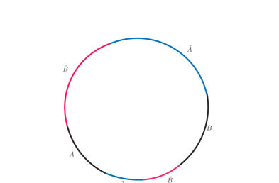
Figure 1: A possible division of $\overline{AB}$ by $\tilde{A}$ (red) and $\tilde{B}$ (blue).

where we have used the cyclic property of trace and the microcausality condition for local algebra, i.e., $[\mathcal{O}(x),\mathcal{O}(y)]=0$ when $x$ and $y$ are spacelike separatedHaag . Since (II) is true for any operator $\mathcal{O}_{AB}$, using the Reeh-Schlieder theorem again, there should exist an operator $\mathcal{O}_{AB}$ such that $\mathcal{O}_{AB}|0\rangle=(\mathcal{O}_{\overline{AB}}\mathcal{O}^{\dagger}_{\overline{AB}}-{\bf{1}})|0\rangle$ and $\mathcal{O}_{AB}|0\rangle=(\mathcal{O}^{\dagger}_{\overline{AB}}\mathcal{O}_{\overline{AB}}-{\bf{1}})|0\rangle$. Therefore, by using (II), the norm of states $(\mathcal{O}_{\overline{AB}}\mathcal{O}^{\dagger}_{\overline{AB}}-{\bf{1}})|0\rangle$ and $(\mathcal{O}^{\dagger}_{\overline{AB}}\mathcal{O}_{\overline{AB}}-{\bf{1}})|0\rangle$ are vanishingExplain2 . Finally, we have

$$\mathcal{O}^{\dagger}_{\overline{AB}}\mathcal{O}_{\overline{AB}}=\mathcal{O}_{\overline{AB}}\mathcal{O}^{\dagger}_{\overline{AB}}={\bf{1}}.$$ (8)

Now we arrive at our main result in this section.
 
Corollary 1:
The set of the purifications of reduced density matrix $\rho_{AB}$ can be approximated by the Hilbert space $\mathcal{H}_{\psi}$ constructed by acting unitary local operators $\mathcal{U}_{\overline{AB}}$ on the vacuum, i.e.,

$$\mathcal{H}_{\psi}=\{\mathcal{U}_{\overline{AB}}|0\rangle,\quad\text{unitrary}\quad\mathcal{U}_{\overline{AB}}\in\mathscr{R}(\overline{AB})\}.$$ (9)

III Surface/State Correspondence and proof of Holographic EoP

Even though we have constrained the set of the purifications to be $\mathcal{H}_{\psi}$, it is still hard to find the minimization of $S_{A\tilde{A}}$ by directly calculating in field theory. In the paper Miyaji:2015yva the authors proposed a new duality relation between a bulk codimension-2 spacelike surface and quantum states in the dual field theory, which is expected to be a generalization of original AdS/CFT. In the context of surface/state correspondence, the gravity lives on a manifold $M_{d+2}$, any codimension-2 convext surface $\Sigma$ corresponds to state in the total Hilbert space $\mathcal{H}$. In this paper we would work in AdS₃, the states are represented by curves $\sigma$ in AdS space. We would like to summarize the three important points of this correspondence:
1. A pure state $|\Phi(\sigma)\rangle$ corresponds to topologically trivial curve, i.e., homologous to a point, in the bulk.
2. If two curves $\sigma_{1}$ and $\sigma_{2}$ are connected by a smooth deformation that preserves convexity, the corresponding states of them are related by a unitary transformation, that is

$$|\Phi(\sigma_{1})\rangle=U(1,2)|\Phi(\sigma_{2})\rangle,$$ (10)

where $U(1,2)$ is a unitary operator associated with deformation pathes.
3. The entanglement entropy for a subregion $\sigma_{A}$ of the curve $\sigma$ is conjectured to be given by the area formula,

$$S_{\sigma,A}=\frac{\text{min}\{\text{area}(\gamma_{\sigma,A})\}}{4G},$$ (11)

where $G$ is the Newton constant.
If taking the curve $\sigma$ to be AdS boundary, these would be the AdS/CFT correspondence, specially the entanglement entropy is RT formula. According to Corollary 1, we are interested in the unitary transformation $\mathcal{U}_{\overline{AB}}$ that act on subregion $\overline{AB}$. In the bulk these transformations are dual to deformations of curve on the AdS boundary while keeping the boundary of $\overline{AB}$ invariant. Note that for a unitary operator $\mathcal{U}_{A}$ located in a subregion $A$ acting on the state $\Phi(\sigma)$, the corresponding deformation of surface $\sigma$ cannot transcend the extremal surface $\gamma_{\sigma,A}$. Only in this way one could keep the convexity of the deformed curves, and this also guarantees the holographic entanglement entropy of subregion $A$ is invariant under unitary transformation $\mathcal{U}_{A}$Miyaji:2015yva .
Now we are ready to prove the holographic EoP based on the surface/state correspondence. For simplicity we choose $A$ and $B$ to be two disconnected interval as shown in Fig.2.
If $A$ and $B$ are far away from each other, the entanglement wedge $W_{AB}$, defined by a region surrounded by $A$, $B$ and the minimal surface $\gamma_{A,B}$ homologous to them, would become disconnected, see Fig.2 . In this case we may choose a series of deformations of the curve $\tilde{A}(\lambda)$ and $\tilde{B}(\lambda)$. Since these deformations correspond to unitary transformations $\mathcal{U}_{\overline{AB}}$, they just need to keep the boundary of $\tilde{A}(\lambda)\tilde{B}(\lambda)$ invariant. As shown in the Fig.2 we always could choose a series of deformations $\tilde{A}(\lambda_{n})$ and $\tilde{B}(\lambda_{n})$ such that $\tilde{A}(\lambda_{\infty})=\lim_{n\to\infty}\tilde{A}(\lambda_{n})$ becomes connected in the bulk. Recall the definition of EoP (2), it is equal to the minimal value of entanglement entropy $S_{A\tilde{A}}$. The holographic entanglement entropy for $A\tilde{A}(\lambda_{n})$ is given by (11). Therefore, we get $S_{A\tilde{A}(\lambda_{\infty})}=0$Explain3 . This means the holographic EoP is zero. Note that in the Fig.2 we only draw a special example for the deformations. In principle, there exist infinite ways to make $S_{A\tilde{A}(\lambda_{\infty})}=0$. For example the deformations corresponding to $\mathcal{U}_{\tilde{A}}$ or $\mathcal{U}_{\tilde{B}}$ would never effect the value of $S_{A\tilde{A}(\lambda_{n})}$.
If the entanglement wedge $W_{AB}$ becomes connected as shown in Fig.3, a series of deformations $\tilde{A}(\lambda)$ and $\tilde{B}(\lambda)$ corresponding to the unitary transformations $\mathcal{U}_{\overline{AB}}$ still keep the boundary of $\tilde{A}(\lambda)\tilde{B}(\lambda)$ invariant. One of the examples is shown in Fig.3. In this case the curve of $\tilde{A}(\lambda_{n})$ would never possible become connected, since the deformation should never transcend the extremal surface $\gamma_{AB}$. Suppose $\Sigma_{AB}$ is the extremal surface as well as minimal area with the end points on the extremal surface $\gamma_{AB}$.

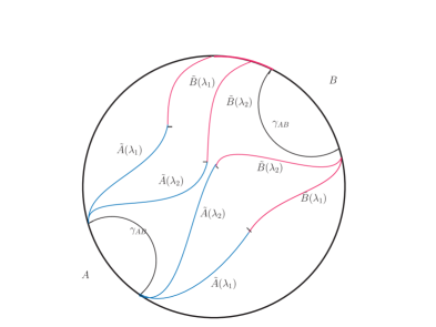
Figure 2: A series of deformation of $\tilde{A}$ (blue) and $\tilde{B}$ (red) for the disconnected entanglement wedge.

Therefore, to get the minimal value of $S_{A\tilde{A}}$ one could construct a series of deformations such that the end points of $\tilde{A}(\lambda_{\infty})=\lim_{n\to\infty}\tilde{A}(\lambda_{n})$ coincide with the ones of $\Sigma_{AB}$. In this limit we would have the minimal value of $S_{A\tilde{A}}$ which is given by

$$S_{A\tilde{A}(\lambda_{\infty})}=\frac{\Sigma_{AB}}{4G}.$$ (12)

Therefore, we have proved the holographic EoP in the context of surface/state correspondence. In above discussion we only focus on two intervals case, but it is straightforward to generalize the proof to more complicated cases. The holographic generalization to muti-partite correlations is discussed in Umemoto:2018jpc .

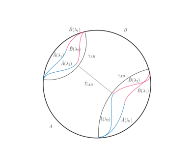
Figure 3: A series of deformation of $\tilde{A}$ (blue) and $\tilde{B}$ (red) for the connected entanglement wedge.

IV Projective Measurement and EoP in CFT

Another interesting question is what kinds of unitary operators $\mathcal{U}_{\overline{AB}}$ would produce the minimal value of $S_{A\tilde{A}}$. Firstly, we should note that the unitary operator is not unique, if $\mathcal{\tilde{U}}_{\overline{AB}}$ is one, so are the operators $\mathcal{U}_{\bar{A}}\mathcal{\tilde{U}}_{\overline{AB}}$ and $\mathcal{U}_{\bar{B}}\mathcal{\tilde{U}}_{\overline{AB}}$. It is still an open question whether the operator is unique up to the above gauge.
In this section we will discuss one special operator belonging to the algebra $\mathscr{R}(\overline{AB})$, that is the projective measurement in CFT. The projective measurement in 1+1 dimensional CFT was discussed in Rajabpour:2015uqa Rajabpour:2015xkj Najafi:2016kwb , its holographic explanation and applications can be found in Numasawa:2016emc . We focus on the projective measurement $\mathcal{P}^{\alpha}_{\overline{AB}}$, which makes the states in the region $\overline{AB}$ fixed by some conformal bases $\alpha$. For example, for free boson theory, a projective measurement with fixed $\phi$ in region $A$ corresponds to Dirichlet boundary condition on $A$, which is a conformal boundary.
Note that the projective measurements $\mathcal{P}^{\alpha}_{\overline{AB}}$ are not unitary. But as we will show soon the entanglement entropy $S_{A\tilde{A}}$ with $\tilde{B}=\overline{AB}$ is very close to the holographic EoP.
We would follow the results in Najafi:2016kwb , there the author considered the projective measurement is for two intervals as shown in Fig.4. The projective state $\mathcal{P}_{\tilde{B}}|0\rangle$ can be represented by path integral on the lower half plane with two slits on $\tilde{B}_{1}$ and $\tilde{B}_{2}$. Assume the length of the intervals $l_{\tilde{B}_{1}}=s_{1}$, $l_{\tilde{B}_{2}}=s_{2}$ and $l_{A}=l$. To calculate Rényi entropy $S^{n}_{A}$ for subsystem $A$ in the state $\mathcal{P}_{\tilde{B}}|0\rangle$ we need to evaluate the path integral on the n-sheet surface $\Sigma_{n}$ with two slits $\tilde{B}_{1}$,$\tilde{B}_{2}$ and branch cut on $A$. The Rényi entropy is given by

$$S_{A}^{n}=\frac{1}{1-n}\log\frac{\mathcal{Z}_{\Sigma_{n}}}{\mathcal{Z}_{\Sigma_{1}}^{n}},$$ (13)

where $\Sigma_{1}$ is the surface with two slits. The entanglement entropy is just $S_{A}=\lim_{n\to 1}S^{n}_{A}$. The partition function $\mathcal{Z}_{\Sigma_{n}}$ can be calculated throw a conformal mapping $w_{n}(z)$ from $\Sigma_{n}$ to annulus, see Appendix of Rajabpour:2015xkj for the detail of the mapping.

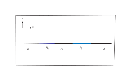
Figure 4: The state with projective measurement in region $\tilde{B}:=\tilde{B}_{1}\tilde{B}_{2}$ (blue line) can be represented by path integral on the lower half plane with two slits.

For general $s_{1},s_{2},l$ there are no analytical results . In the limit $l\gg s_{1}=s_{2}=s$ the result is

$$S_{A}=\frac{c}{3}\log\frac{l}{s}+...,$$ (14)

where $...$ denote the contributions from the boundary, which are not related to central charge $c$. In the limit $l\ll s_{1}=s_{2}=s$, $S_{A}=0$ up to some boundary contributions.
In the limit $s_{2}\ll s_{1},l$,

$$S_{A}=\frac{c}{6}\log\frac{l(l+s_{1})}{s_{1}s_{2}}+...,$$ (15)

with $...$ being the boundary contributions.
Now we would like to compare the entanglement entropy after projective measurement with holographic EoP for $AB$. In the limit $l\ll s_{1}=s_{2}=s$, the entanglement wedge of $AB$ becomes disconnected, the holographic EoP is vanishing. The entanglement entropy after projective measurement is also vanishing up to some boundary contributions.
In the limit $l\gg s_{1}=s_{2}=s$ or $s_{2}\ll s_{1},l$ the entanglement wedge of $AB$ should be connected. In the appendix we calculate the holographic EoP for the interval $A$ and $B$, the result is

$$E_{AB}=\frac{c}{6}\log\Big{[}\frac{s_{1}\left(2l+s_{2}\right)}{s_{1}s_{2}}$$

$$+\frac{2\left(l^{2}+ls_{2}+\sqrt{l\left(l+s_{1}\right)\left(l+s_{2}\right)\left(l+s_{1}+s_{2}\right)}\right)}{s_{1}s_{2}}\Big{]}.$$ (16)

The holographic EoP is

$$E_{AB}=\left\{\begin{aligned} &&\frac{c}{3}\log\frac{2l}{s},\ \text{in the limit}\ l\gg s_{1}=s_{2}=s\\ &&\frac{c}{6}\log\frac{4l\left(l+s_{1}\right)}{s_{1}s_{2}},\ \text{in the limit}\ s_{2}\ll s_{1},l.\end{aligned}\right.$$

Comparing with the results of projective measurement (14) and (15) in the same limit, we find that their difference is $\frac{c}{3}\log 2$. This suggests the projective measurement operator may provide as an approximate operator of the unitary operator that produces the minimal value of $S_{A\tilde{A}}$.

V Discussions

Our discussions are mainly for vacuum state, but it is straightforward to generalize to other cyclic state, such as the states on which the translation group acts homorphicallyWitten:2018lha . For mixed state in 1+1 dimension CFT the thermal state is conformal equal to the vacuum state, our discussions may be generalized to that case. This may fail for non-entangled state, such as the boundary state in CFTCardy Miyaji:2014mca .
Our proof of holographic EoP only includes the states that can be described by geometry in the bulk. At least in 2D CFT it is expected there are many states that cannot be dual to a classical geometryGuo:2018fnv . So the proof is only true for the class of geometric states.
The small difference between holographic EoP and entanglement entropy after projective measurement may be understood along with holographic explanation of projective measurementNumasawa:2016emc . We would explore more on this in the near future.
 
 I would like to thank Pak Hang Chris Lau for discussions. I also would like to thank the organisers of the NCTS Annual Meeting 2018: Particles, Cosmology and String. Tadashi Takayanagi’s talk at this conference brought my attention to entanglement of purification. I am supported in part by the National Center of Theoretical Science (NCTS).

Appendix A Holographic EoP of two intervals in 1+1 dimensional CFT

We will derive the holographic EoP of two intervals in 1+1 dimensional CFT in this section. To compare with the result in the main tex we choose $A$ and $B$ as shown in Fig.4. We only plot the case when $AB$ has connected entanglement wedge in Fig.5. To calculate holographic EoP we need to compute the length of the entanglement wedge cross section, i.e., $\Sigma_{AB}$ in Fig.5. The minimal length condition leads to the curve $\Sigma_{AB}$ is perpendicular to the extremal surface of entanglement wedge at the points $(x_{1},z_{1})$ and $(x_{2},z_{2})$. With some simple calculations we get

$$z_{1}=\frac{s_{1}\sqrt{l\left(l+s_{1}\right)\left(l+s_{2}\right)\left(l+s_{1}+s_{2}\right)}}{s_{1}^{2}+2l\left(l+s_{2}\right)+s_{1}\left(2l+s_{2}\right)}$$

$$z_{2}=\frac{s_{2}\sqrt{l\left(l+s_{1}\right)\left(l+s_{2}\right)\left(l+s_{1}+s_{2}\right)}}{2l^{2}+2l\left(s_{1}+s_{2}\right)+s_{2}\left(s_{1}+s_{2}\right)},$$ (17)

and the equation of the curve $\Sigma_{AB}$, $(x-x_{0})^{2}+z^{2}=z_{*}^{2}$ with

$$x_{0}=\frac{l(s_{2}-s_{2})}{2(2l+s_{1}+s_{2})}$$

$$z_{*}=\frac{\sqrt{l\left(l+s_{1}\right)\left(l+s_{2}\right)\left(l+s_{1}+s_{2}\right)}}{2l+s_{1}+s_{2}}.$$ (18)

The length of $\Sigma_{AB}$ is

$$L=\log\Big{[}\frac{s_{1}\left(2l+s_{2}\right)}{s_{1}s_{2}}$$

$$+\frac{2\left(l^{2}+ls_{2}+\sqrt{l\left(l+s_{1}\right)\left(l+s_{2}\right)\left(l+s_{1}+s_{2}\right)}\right)}{s_{1}s_{2}}\Big{]}.$$ (19)

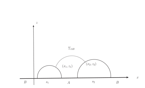
Figure 5: Calculations of holographic EoP for two interval $A$ and $B$ with $l_{A}=l$ and the distances between $A$, $B$ are $s_{1}$ and $s_{2}$.

References

- (1) J. M. Maldacena, Int. J. Theor. Phys. 38, 1113 (1999) [Adv. Theor. Math. Phys. 2, 231 (1998)] [hep-th/9711200].
- (2) S. Ryu and T. Takayanagi, Phys. Rev. Lett. 96, 181602 (2006) [hep-th/0603001].
- (3) V. E. Hubeny, M. Rangamani and T. Takayanagi, JHEP 0707, 062 (2007) [arXiv:0705.0016 [hep-th]].
- (4) R. Haag, Local quantum physics: Fields, particles, algebras. Springer Science Business Media, 2012.
- (5) R. F. Streater and A. S. Wightman, PCT, spin and statistics, and all that. Princeton University Press,2016.
- (6) B. M. Terhal, M. Horodecki, D. W. Leung and D. P. DiVincenzo, Journal of Mathematical Physics, 43(9), 4286-4298 (2002). [arXiv:0202044[quant-ph]]
- (7) T. Takayanagi and K. Umemoto, Nature Phys. 14, no. 6, 573 (2018) [arXiv:1708.09393 [hep-th]].
- (8) P. Nguyen, T. Devakul, M. G. Halbasch, M. P. Zaletel and B. Swingle, JHEP 1801, 098 (2018) [arXiv:1709.07424 [hep-th]].
- (9) B. Czech, J. L. Karczmarek, F. Nogueira and M. Van Raamsdonk, Class. Quant. Grav. 29, 155009 (2012) [arXiv:1204.1330 [hep-th]].
- (10) A. C. Wall, Class. Quant. Grav. 31, no. 22, 225007 (2014) [arXiv:1211.3494 [hep-th]].
- (11) M. Headrick, V. E. Hubeny, A. Lawrence and M. Rangamani, JHEP 1412, 162 (2014) [arXiv:1408.6300 [hep-th]].
- (12) X. Dong, D. Harlow and A. C. Wall, Phys. Rev. Lett. 117, no. 2, 021601 (2016) [arXiv:1601.05416 [hep-th]].
- (13) P. Caputa, M. Miyaji, T. Takayanagi and K. Umemoto, arXiv:1812.05268 [hep-th].
- (14) J. Hauschild, Johannes, E. Leviatan; J. Bardarson, E. Altman, M. Zaletel, F. Pollmann, Finding purifications with minimal entanglement , eprint arXiv:1711.01288
- (15) A. Bhattacharyya, T. Takayanagi and K. Umemoto, JHEP 1804, 132 (2018) [arXiv:1802.09545 [hep-th]].
- (16) M. Miyaji and T. Takayanagi, PTEP 2015, no. 7, 073B03 (2015) [arXiv:1503.03542 [hep-th]].
- (17) M. Miyaji, T. Numasawa, N. Shiba, T. Takayanagi and K. Watanabe, Phys. Rev. Lett. 115, no. 17, 171602 (2015) [arXiv:1506.01353 [hep-th]].
- (18) M. A. Rajabpour, Phys. Rev. B 92, no. 7, 075108 (2015) [arXiv:1501.07831 [cond-mat.stat-mech]].
- (19) M. A. Rajabpour, J. Stat. Mech. 1606, no. 6, 063109 (2016) [arXiv:1512.03940 [hep-th]].
- (20) B. S. Kay and R. M. Wald, Physics Reports, 207(2), 49-136 (1991).
- (21) E. Witten, Rev. Mod. Phys. 90, no. 4, 045003 (2018) [arXiv:1803.04993 [hep-th]].
- (22) More precisely, for any state one always could find an operator such that the , where is an aribrary positive constant.
- (23) In fact this follows by another important property of vacuum state, that is the separating property. A state is said to be separating for the local algebra if .
- (24) The original state corresponding to is a mixed state, since it is a part of a closed surface, i.e., AdS boundary. Under a series of unitary transformations, the state would approach to a pure state. This is consistent with the intuition of purification process.
- (25) K. Umemoto and Y. Zhou, JHEP 1810, 152 (2018) [arXiv:1805.02625 [hep-th]].
- (26) K. Najafi and M. A. Rajabpour, JHEP 1612, 124 (2016) [arXiv:1608.04074 [cond-mat.str-el]].
- (27) T. Numasawa, N. Shiba, T. Takayanagi and K. Watanabe, JHEP 1608, 077 (2016) [arXiv:1604.01772 [hep-th]].
- (28) J. L. Cardy, Boundary Conditions, Fusion Rules and the Verlinde Formula, Nucl. Phys. B 324 (1989) 581.
- (29) M. Miyaji, S. Ryu, T. Takayanagi and X. Wen, JHEP 1505, 152 (2015) [arXiv:1412.6226 [hep-th]].
- (30) W. Z. Guo, F. L. Lin and J. Zhang, arXiv:1806.07595 [hep-th].