Perfectly matched layers simulation in 2-D VTI media

Abstract

Implementing computational boundary conditions, such as perfectly matched layers PML does have advantages for forwarding modeling of the earth’s crust. The mathematical modeling of many physical problems encountered in industrial applications often leads to a system of linear partial differential equations PDEs. It considerably improves the visualization of seismic events relevant to oil and gas exploration. In this work, we present an efficient numerical scheme for hyperbolic partial differential equations where a computational technique takes care of reflections at the border s domain using a linear 2-D elastic-wave system of decoupled equations with PML-type boundary conditions. The key idea is to introduce a layer that absorbs the reflections from the borders improving images visualization. Anisotropy has been reported to occur in the Earth’s three main layers. The crust, the mantle, and the core; but this implementation refers to the case of a vertical transversal anisotropic medium VTI in the crust-layer. Images and screen-shots of the longitudinal P impulse-response and the SV transverse impulse-response are obtained at different times. This computational method enables us to achieve images for the P and SV response-impulses, and to obtain high quality synthetic seismograms for the PP and PS reflection events in a 2-D VTI two-layer model.

Keywords: Seismic anisotropy, VTI medium, computational modeling, perfectly matched layer.

Introduction

The wave equation plays an important role in seismic oil and gas exploration since it allows modeling the earth structure. In the past decades, seismic anisotropy has been gaining attention from academic and industry, in part thanks to advances in anisotropy parameter estimation gre3 ; gre2

A material is said to be anisotropic if the value of one or more of its properties varies with direction, consequently anisotropy consideration improves the subsurface imaging. Seismic Anisotropy can be defined as the dependence of seismic velocity on a direction or upon an angle. Anisotropy is described by a $4^{th}$ order elasticity tensor with 21 independent components for the lowest-symmetry case hel ; mus ; lan ; del . However in practice, observational studies are unable to distinguish all 21 elements and anisotropy considerations are usually simplified. For seismic exploration, the most complicated case occurs in fractured monoclinic media, with 9 elastic constants gre . In general, two or more sets of vertical non-corrugated and not perpendicular fractures produce an effective monoclinic medium with a horizontal symmetry plane. The second most important application occurs for the orthorhombic model. The orthorhombic model describes a layered medium fracture in two orthogonal directions tsv ; con2 , However in the simplest form that seismic exploration uses it, there are two main kinds of transverse anisotropy TI. One is called horizontal transverse isotropy-HTI which is a common model in shear-wave studies of fractured reservoirs that describes a system of parallel vertical penny-shaped cracks embedded in an isotropic host rockcon1 , henceforth this kind of anisotropy is associated with cracks and fractures. The other one is called vertical transversal anisotropy-VTI thom and it is associated with layering and shales. Sometimes people call it vertical polar anisotropy.

In the beginning, forward modeling was done by simulating the scalar $P$ wave field obtained from the acoustic wave equation. However, the earth-crust is elastic and anisotropic hel ; gre ; con2 and all propagation modes should be considered in order to observe anisotropy effects. Forward modeling and parameter estimation are almost the most fundamental to all other anisotropy applications in oil exploration gre2 . In part, this can be done by numerically solving the hyperbolic elastic wave equation WE. The vector and tensor fields which represent the WE improves the information about the 3D earth-crust geology. This translates into a better subsurface imaging and it is of extreme importance for the oil and gas seismic exploration.

The most common type of anisotropy that occurs in the earth’s crust is the vertical transverse anisotropy VTI which is observed in sedimentary rocks winterstein . To achieve 3D seismic modeling with VTI anisotropy requires the knowledge of five elastic constants. However in two dimensions only four constants are involved, namely $C_{11}$, $C_{33}$, $C_{13}$ and $C_{44}$ (in this work we use Voigt notation for the elastic constants) faria ; thom . Henceforth shear wave splitting is not considered in a 2-D modeling because of the lack of the elastic constant $C_{66}$. Abundant geological evidence of shales shows the importance of VTI models in seismic reservoir characterization gre3 ; gre2 .

In this work, we implement an algorithm using a linear finite difference decoupled PDEs in terms of the velocities and stress tensor components. To implement such a model we use central-difference second order approximation for space variables and time partial derivatives. Henceforth we use the finite-difference time-domain FDTD method yee . In addition, we use staggered stencils for computational storage virieux . Staggered cells grant the calculation of different physical quantities at different mesh-grid points (see Figure 2), reducing the computational cost storage. Additionally, with this algorithm we can introduce different source-receiver configurations, making it ideal for simulation in oil and gas seismic modeling.

To implement a FDTD solution of the WE, a computational frame must first be established. The computational domain is the physical region over which the simulation is performed. To achieve the condition of non-reflective borders, we use the artificial technique of perfectly coupled layers PML festa ; dimitri . Consequently, the effect due to the reflection of the waves at the borders of the domain is automatically reduced.

PML implementation in seismic exploration requires a reformulation of the linear WE to eliminate the unwanted reflections. Thus, this work is structured in the following way: Section I introduces the topic of seismic anisotropy and its relevant application in R&D Oil industry. Section II briefly describes the PDEs for a 2-D medium with VTI shale anisotropy, and the theoretical implementation of the PML obtaining a decoupled EWs (elastic equation system) including the new border computational conditions. Section III describes the numerical implementation that will allow CPU time reduction. Subsequently, we find the correct decoupled finite-difference scheme in terms of the staggered-stencil mesh taking into consideration the PML (see Figure 2). Finally, in section IV the outcome shows the applicability of this technique. We were able to achieve very neat and sharp subsurface images without reflection events at the edges of the 2-D earth-crust two dip layer shale model.

2-D linear VTI media

As we stated before, the formulation of a linear WEs in terms of temporal derivatives of the velocity and the stress fields can be used to propagate waves. The FDTD technique reproduces the fields forward in time-domain. This is called forward modeling. This procedure is designed through a 3D staggered finite-difference grid faria . This formulation is widely used in the literature for seismology purposes virieux . In 2-D VTI anisotropy, it involves the transformation of five coupled first-order PDEs, namely the two general equations of motion for the vector velocity $(v_{x},v_{z})$ field which are:

$$\rho\frac{\partial v_{x}}{\partial t}=f_{x}+\frac{\partial\sigma_{xx}}{\partial x}+\frac{\partial\sigma_{xz}}{\partial z},\qquad\rho\frac{\partial v_{z}}{\partial t}=f_{z}+\frac{\partial\sigma_{xz}}{\partial x}+\frac{\partial\sigma_{zz}}{\partial z},$$

where $\rho$ is a constant density, $f_{x}$ and $f_{z}$ are external forces driven by the source. Since we use the FDTD time-domain technique, a seismic pulse is used as the source, then the response of the system over a wide range of frequencies can be obtained with a single simulation.

And the three equations for the stress $\sigma_{ij}$ second order tensor field

$$\sigma_{ij}=\left[{\begin{array}[]{cc}\sigma_{xx}&\sigma_{xz}\\ \sigma_{zx}&\sigma_{zz}\\ \end{array}}\right]$$

where only four elastic constants are used as the input variables for the WEs:

$$\frac{\partial\sigma_{xx}}{\partial t}=c_{11}\;\frac{\partial v_{x}}{\partial x}+c_{13}\;\frac{\partial v_{z}}{\partial z},\qquad\frac{\partial\sigma_{zz}}{\partial t}=c_{33}\;\frac{\partial v_{z}}{\partial z}+c_{13}\;\frac{\partial v_{x}}{\partial x},\;\qquad\frac{\partial\sigma_{xz}}{\partial t}=c_{44}\;\Big{[}\frac{\partial v_{x}}{\partial z}+\frac{\partial v_{z}}{\partial x}\Big{]},$$

the longitudinal $P$ and the transverse $SV$ modes given by the previous five PDEs are coupledfaria .

2-D VTI decoupled PDEs with PML

In this subsection, the PML technique is briefly explained and applied to the 2-D modeling. In order to make the finite difference method more stable and convergent, we follow the arguments presented previouslyfesta ; dimitri for the stability and the dispersion conditions in a 2-D EWs (we should mention that a 3D anisotropy implementation has not been achieved with this technique, due to failures in the stability and dispersion conditions when considering anisotropyfaria ). Even in works dedicated to seismology, the use of this technique helps to improve 2-D imaging resolution at larger scales. The seismological domains have borders as it happens in seismic exploration. PML in this case, reduces the reflections at the borders in a significant amount compared with the use of traditional mathematical boundary conditions .

The PML mathematical implementation consist in the introduction of a modified coordinate system, where the expansion coefficient is a complex number with an evanescent imaginary part. This generalization is achieved through the following substitution

$$\frac{\partial}{\partial x}\rightarrow\frac{1}{1+i\;\frac{p(x)}{\omega}}\;\frac{\partial}{\partial x},$$

and

$$\frac{\partial}{\partial z}\rightarrow\frac{1}{1+i\;\frac{p(z)}{\omega}}\;\frac{\partial}{\partial z},$$

where $p(x)$ and $p(z)$ are the coefficients of the PML. They are given by the following expressions dimitri

$$p(x)=p_{0}\;(x/L)^{N},\;and\;p(z)=p_{0}\;(z/L)^{N},$$

with $p_{0}$ $=$ $-3\;v_{p}\;logR_{c}/(2\;L)$, where $L$ is the thickness of the perfectly coupled layer, $N$ the size of the problem and $p_{0}$ has an approximate value of 341.9

When the above coordinate system is replaced in the equations for the VTI medium of the previous section, the system becomes a new linear decoupled PDE-EWs. Because of that replacement appears new equations for $v^{1}_{x}$ and $v^{2}_{x}$ new decoupled velocities:

$$\rho\;\Big{[}\frac{\partial}{\partial t}+p(x)\Big{]}v^{1}_{x}=f_{x}+\frac{\partial\sigma_{xx}}{\partial x},\qquad\rho\;\Big{[}\frac{\partial}{\partial t}+p(z)\Big{]}v^{2}_{x}=\frac{\partial\sigma_{xz}}{\partial z},$$

For the decoupled $v^{1}_{z}$ and $v^{2}_{z}$ velocities the equations are:

$$\rho\;\Big{[}\frac{\partial}{\partial t}+p(x)\Big{]}v^{1}_{z}=f_{z}+\frac{\partial\sigma_{xz}}{\partial x},\qquad\rho\;\Big{[}\frac{\partial}{\partial t}+p(z)\Big{]}v^{2}_{z}=\frac{\partial\sigma_{zz}}{\partial z}.$$

These decoupled velocities dimitri are related to the coupled ones by the relation $v_{x}=v^{1}_{x}+v^{2}_{x}$ and $v_{z}=v^{1}_{z}+v^{2}_{z}$.

The stress tensor field is mathematically treated in the same way, obtaining a decoupled system for the new stress equations: The new decoupled $\sigma^{1}_{xx}$ and $\sigma^{2}_{xx}$ stress equations are:

$$\Big{[}\frac{\partial}{\partial t}+p(x)\Big{]}\sigma^{1}_{xx}=c_{11}\;\frac{\partial v_{x}}{\partial x},\qquad\Big{[}\frac{\partial}{\partial t}+p(z)\Big{]}\sigma^{2}_{xx}=c_{13}\;\frac{\partial v_{z}}{\partial z},$$

and the new equations for the $\sigma^{1}_{zz}$ and $\sigma^{2}_{zz}$ decoupled stress tensors components equal to:

$$\Big{[}\frac{\partial}{\partial t}+p(x)\Big{]}\sigma^{1}_{zz}=c_{13}\;\frac{\partial v_{x}}{\partial x},\qquad\Big{[}\frac{\partial}{\partial t}+p(z)\Big{]}\sigma^{2}_{zz}=c_{33}\;\frac{\partial v_{z}}{\partial z}.$$

The decoupled shear $\sigma^{1}_{xz}$ and $\sigma^{2}_{xz}$ stress tensor components follow the equations:

$$\Big{[}\frac{\partial}{\partial t}+p(x)\Big{]}\sigma^{1}_{xz}=c_{44}\;\frac{\partial v_{z}}{\partial x},\qquad\Big{[}\frac{\partial}{\partial t}+p(z)\Big{]}\sigma^{2}_{xz}=c_{44}\;\frac{\partial v_{x}}{\partial z}.$$

where now $\sigma_{xx}=\sigma^{1}_{xx}+\sigma^{2}_{xx}$, $\sigma_{zz}=\sigma^{1}_{zz}+\sigma^{2}_{zz}$, and $\sigma_{xz}=\sigma^{1}_{xz}+\sigma^{2}_{xz}$. These 5 linear PDE equations will be used for a forward modeling in the following section.

Computational space time implementation

The computational model that we propose in this simulation is divided into a mesh of $N_{x}$ $\times$ $N_{z}$ points. Fig. (1) the finite-difference scheme shows the computational edge domain where the PML are applied according to the two-layer dip model. $\Delta x$ and $\Delta z$ are defined as the distances between the points in such a way that $x=n_{x}\Delta_{x}$ y $z=n_{z}\Delta z$ with $n_{x}=1...N_{x}$ y $n_{z}=1...N_{z}$. For the step in time $\Delta t$ we have that $t=n\Delta t$, being $n$ the step time (in Fig. 2) the stencil time is not showed faria .

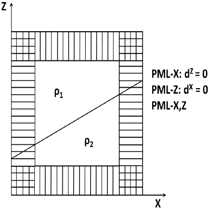
Figure 1: Finite-difference simplified scheme showing the computational 2 two-layer dip model. The vertical, horizontal and crossed lines near the borders show where the PLM are applied

The five variables $v^{1}_{x}$, $v^{1}_{z}$, $\sigma^{1}_{xx}$, $\sigma^{1}_{zz}$, and $\sigma^{1}_{xz}$ are discretize into a two dimensional staggered grid mesh, see Fig. (2) for a better explanation, where the velocity components are stored in both stencils, the normal components of the stress tensors are stored in one of the stencils, while the shear stress components are located at another stencil. However, the major difference of a staggered-grid scheme is that the velocity and stress components are not known at the same grid point, as it can be seen from Fig. (2), henceforth we use a previous scheme proposal with little modifications faria where different stencils are used for normal and shear stress field computations.

Following Fig. (2) in the space domain $v_{x}$ is calculated at the points $(i\pm 1/2,k)$, $v_{z}$ is calculated at the points $(i,k\pm 1/2)$, the normal stress tensor components $\sigma_{xx}$ and $\sigma_{zz}$ are calculated at the points $(i,k)$ and finally the shear stress $\sigma_{xz}$ is calculated at the points $(i\pm 1/2,k\pm 1/2)$. The density $\rho(x,y,z)$ is considered a constant density $\rho_{0}$ (see the last line of Table I for its correspondent values and units) Physically it means that the VTI model is homogeneous and that is does not take into consideration earth-crust heterogeneities.

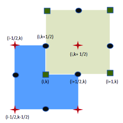
Figure 2: Staggered finite-difference grid for the velocity and stress updates, both stencils show the grids points where different fields components are calculated. Velocity components are calculated in both stencils (black circles), the shear stress components are calculated in the blue stencil (red starts), and the cinnamon stencil is used to calculate the normal stress components (green squares).

An explosive source is simulated using the amplitude of a Ricker wavelet with a peak frequency $f_{0}\sim 30$ Hertz. Amplitudes are added to the velocities $v^{1}_{x}$ and $v^{1}_{z}$ at each $n$ time-step. The stability limit of the discrete system is given by the following condition:

$$\Delta t\;<0.606\;\frac{\Delta x}{V_{p}},$$

where $V_{p}$ account s for the horizontal longitudinal speed faria . The dispersion condition for the discrete system is given by the inequality:

$$\Delta x\;<\;\frac{V_{s}}{10\;f_{0}},$$

where $V_{s}$ is the transverse wave speed. However some authors Becache showed that the stability of the classical PML model depends upon the physical properties of the anisotropic medium and that it can be intrinsically unstable. However the elastic constants in table 1 where previously provenfaria to meet Becache stability criteria. This algorithm could be extended to 3-D situations by further studying the stability and dispersion conditions.

Henceforward we proceed to obtain the discretization of the velocity fields as follows for the decoupled finite-difference system: the $v^{1}_{x}$ and the $v^{2}_{x}$ components are computed at time-steps points $t^{n+1}$ and $t^{n}$ (the stencil-time is not shown herefaria ) with the following finite-difference equations:

$$v^{1}_{x}|^{n+1}_{i+1/2,k}=v^{1}_{x}|^{n}_{i+1/2,k}e^{-p(x)\Delta t}+\frac{1}{\rho}\frac{\Delta t}{\Delta x}e^{-0.5\;p(x)\;\Delta t}\Big{[}\sigma_{xx}\Big{|}^{n+1/2}_{i+1,k}-\sigma_{xx}\Big{|}^{n+1/2}_{i,k}\Big{]},$$ (1)

$$v^{2}_{x}|^{n+1}_{i+1/2,k}=v^{1}_{x}|^{n}_{i+1/2,k}e^{-p(z)\Delta t}+\frac{1}{\rho}\frac{\Delta t}{\Delta z}e^{-0.5\;p(z)\;\Delta t}\Big{[}\sigma_{xz}\Big{|}^{n+1/2}_{i+1/2,k+1/2}-\sigma_{xz}\Big{|}^{n+1/2}_{i+1/2,k-1/2}\Big{]}.$$ (2)

The $v^{1}_{z}$ and $v^{2}_{z}$ components are calculated at the times-step $t^{n+1}$ and $t^{n}$ points with the help of equations:

$$v^{1}_{z}|^{n+1}_{i,k+1/2}=v^{1}_{z}|^{n}_{i,k+1/2}e^{-p(x)\Delta t}+\frac{1}{\rho}\frac{\Delta t}{\Delta x}e^{-0.5\;p(x)\;\Delta t}\Big{[}\sigma_{xz}\Big{|}^{n+1/2}_{i+1/2,k+1/2}-\sigma_{xz}\Big{|}^{n+1/2}_{i-1/2,k+1/2}\Big{]},$$ (3)

$$v^{2}_{z}|^{n+1}_{i,k+1/2}=v^{1}_{x}|^{n}_{i,k+1/2}e^{-p(z)\Delta t}+\frac{1}{\rho}\frac{\Delta t}{\Delta z}e^{-0.5\;p(z)\;\Delta t}\Big{[}\sigma_{xx}\Big{|}^{n+1/2}_{i,k+1}-\sigma_{xx}\Big{|}^{n+1/2}_{i,k}\Big{]}.$$ (4)

For the stress fields the discretization is as follows: First, the decoupled equations for the normal stress tensor components $\sigma^{1}_{xx}$ and $\sigma^{2}_{xx}$ are computed at the mesh step-time points $t^{n\pm 1/2}$ using the equations:

$$\sigma^{1}_{xx}|^{n+1/2}_{i,k}=\sigma^{1}_{xx}|^{n-1/2}_{i,k}e^{-p(x)\Delta t}+C_{11}\;\frac{\Delta t}{\Delta x}e^{-0.5\;p(x)\;\Delta t}\Big{[}v_{x}\Big{|}^{n}_{i+1/2,k}-v_{x}\Big{|}^{n}_{i-1/2,k}\Big{]},$$ (5)

and

$$\sigma^{2}_{xx}|^{n+1/2}_{i,k}=\sigma^{2}_{xx}|^{n-1/2}_{i,k}e^{-p(z)\Delta t}+C_{13}\;\frac{\Delta t}{\Delta z}e^{-0.5\;p(z)\;\Delta t}\Big{[}v_{z}\Big{|}^{n}_{i,k+1/2}-v_{z}\Big{|}^{n}_{i,k-1/2}\Big{]}.$$ (6)

Second, the decoupled equation for the normal stress components $\sigma^{1}_{zz}$ and $\sigma^{2}_{zz}$ are computed at the time points $t^{n\pm 1/2}$ by means of the following expressions:

$$\sigma^{1}_{zz}|^{n+1/2}_{i,k}=\sigma^{1}_{zz}|^{n-1/2}_{i,k}e^{-p(x)\Delta t}+C_{13}\;\frac{\Delta t}{\Delta x}e^{-0.5\;p(x)\;\Delta t}\Big{[}v_{x}\Big{|}^{n}_{i+1/2,k}-v_{x}\Big{|}^{n}_{i-1/2,k}\Big{]},$$ (7)

and

$$\sigma^{2}_{zz}|^{n+1/2}_{i,k}=\sigma^{2}_{zz}|^{n-1/2}_{i,k}e^{-p(z)\Delta t}+C_{33}\;\frac{\Delta t}{\Delta z}e^{-0.5\;p(z)\;\Delta t}\Big{[}v_{z}\Big{|}^{n}_{i,k+1/2}-v_{z}\Big{|}^{n}_{i,k-1/2}\Big{]}.$$ (8)

Third, the decoupled equations for the shear $\sigma^{1}_{xz}$ and $\sigma^{2}_{xz}$ components are computed at time points $t^{n\pm 1/2}$ by means of:

$$\sigma^{1}_{xz}|^{n+1/2}_{i+1/2,k+1/2}=\sigma^{1}_{zz}|^{n-1/2}_{i+1/2,k+1/2}e^{-p(x)\Delta t}+C_{44}\;\frac{\Delta t}{\Delta x}e^{-0.5\;p(x)\;\Delta t}\Big{[}v_{z}\Big{|}^{n}_{i+1/2,k}-v_{z}\Big{|}^{n}_{i-1/2,k}\Big{]},$$ (9)

and

$$\sigma^{2}_{xz}|^{n+1/2}_{i+1/2,k+1/2}=\sigma^{1}_{zz}|^{n-1/2}_{i+1/2,k+1/2}e^{-p(z)\Delta t}+C_{44}\;\frac{\Delta t}{\Delta z}e^{-0.5\;p(z)\;\Delta t}\Big{[}v_{x}\Big{|}^{n}_{i,k+1/2}-v_{x}\Big{|}^{n}_{i,k+1/2}\Big{]}.$$ (10)

The elastic constants used for the two-layer model are given according to table 1. These values correspond to different types of VTI media and they are able to accomplish the stability condition using a PML computer domain faria ; dimitri ; Becache .

Table 1: VTI elastic constants for model Fig. 4(A) dimitri

elastic constants ($\times 10^{10}N\;m^{-2}$)	upper layer	bottom layer
$C_{11}$	16.5	16.7
$C_{13}$	5.0	6.6
$C_{33}$	6.2	14.0
$C_{44}$	3.4	6.63
$\rho_{0}$ $(Kg\;m^{-3})$	7.100	3.200

Analysis and Results

The present paper describes a new space-time 2-D methodology with time-step and space-step control to solve 2-D VTI linear decoupled EWs with PML conditions using staggered-grids Fig. 1 and Fig. 2. Henceforth, we develop a computational model for an elastic wave propagation simulation for 2-D VTI anisotropic media, by combining a FDTD method on staggered grids with a PML boundary condition. For that, a High-Performance Linux application in C (over 1,000 lines of code) using Make, GDB and Valgrind s memcheck, to generate and visualize 2-D response-impulses and synthetic seismograms was developed.

We establish that visualization of the impulse-response of the P and SV modes are improved by the PML. As a consequence, unwanted reflections from the borders in Fig. 3 are totally eliminated according to Virieux virieux .

In Fig. 3 simulations were performed with an explosive source (Ricket-wavelength) centered in the middle of the model to eliminate reflections from the edges. In Fig. 3 time screen-shots for $t=0.2,0.3$, and $0.5$ sec. are presented. From those snapshots, we conclude that the PML boundary conditions absorb the reflections from the border, implying an exceptional numerical performance of the computational PML technique. Another conclusion is that the P 2-D response-impulse behave as a simpler quasi-elliptical way in Fig. 3, while the SV response-impulse presents triplications. Moreover, the effects of the VTI elastic constants on SV response-impulses affects the direction of propagation. We observe from the snapshots in Fig. 3 how the value of the elastic constant $C_{13}$ affects the direction of the SV. Triplications in the SV wavefront are modeled. However, one question is not solve yet in this work, the asymmetric behavior of the SV impulse-response in Fig. 3 with respect to the vertical axis.

Subsequently, the explosive source is relocated to the upper central part of the 2-D model sketched in Fig. 4 A. On the surface, fifty receivers are uniformly distributed on both sides of the source. We see how the velocity fields cancel out at the edges of the model in Fig. 4 A. Then we obtain the synthetic seismograms for the two layers model, each of them has different elastic constants values. The synthetic seismograms of the vertical component $V_{z}$ (Fig. 3 B) and the horizontal component $V_{x}$ (Fig. 3 C) are shown with the primary reflections events due to the dip layer.

Henceforth, it remarkably shows the effectiveness of the PML using the decoupled linear system of equations (1)-(10) for 2-D VTI media simulation in Oil and Gas R&D.

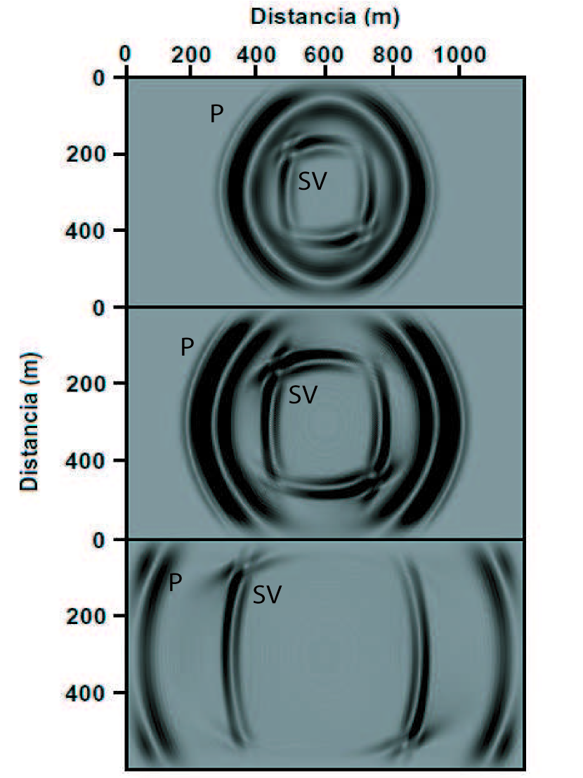
Figure 3: Screen-shots at 0.2, 0.3 and 0.5 sec. are displayed for the vertical velocity wave-field component propagating through a homogeneous medium with elastic constants from the upper layer given in Table I. The triplication of the SV wave around the intermediate angles are observe to be asymmetrical for the SV impulse-response. The absorbing effect of the PML at the edges of the computational domain is notable.

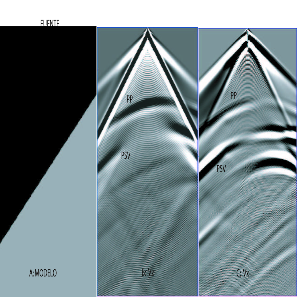
Figure 4: Two-layers VTI dip model 4A. Synthetic seismograms for the vertical Vz are presented in 4B. Synthetic seismograms for the horizontal Vx are displayed in 4C. In 4B and 4C screen-shops for the PP and the PSV reflection events due to the dip are presented.

References

- (1) Perez M., Grechka V., and Michelena R., Geophysics. 64 (1999) 1266.
- (2) Grechka V., and Tsvankin I., Geophysics. 63 (1998) 1079.
- (3) Musgrave, M. Crystal Acoustics. Holden-Day. (1970).
- (4) Helbig, K. Foundations of anisotropic for exploration Geophysics. Pergamon Press. 22 (1994).
- (5) L. D. Landau and E. M. Lifshitz. Elasticity Theory. Pergamon Press, 1982.
- (6) Dellinger, J. Anisotropic seismic wave propagation. Ph.D. thesis. Stanford University, (1991).
- (7) Grechka V., Contreras P. and Tsvankin I., Geophysical Prospecting. 48 (2000) 577.
- (8) Contreras P., Grechka V. and Tsvankin I., Geophysics. 64(4) (1999) 1219.
- (9) Tsvankin I., 66th Ann. Internat. Mtg., Soc. Expl. Geophys. (1996b) 1850.
- (10) Contreras P., Klie H., and Michelena R., 68th Ann. Internat. Mtg. Soc. Expl. Geophys. (1998) 1491.
- (11) L. Thomsen, Geophysics. 51 (1986) 1954.
- (12) D. F. Winterstein, Geophysics. 55, (1990) 1070.
- (13) Faria E. y Stoffa P., Geophysics. 59 (1994) 282.
- (14) Virieux J., Geophysics. 51 (1986) 889.
- (15) Festa G. and Nielsen S. Bulletin of the Seismological Society of America. 93 (2003) 891.
- (16) Komatitsch D. and Martin R., Geophysics. 72 (2007) SM155.
- (17) Kane Y., IEEE Transactions on Antennas and Propagation. 14(3) (1966) 302.
- (18) Becache E., Fauqueux S., and Joly P., J. Comput. Phys. 188 (2003) 399.