Spontaneously broken symmetry restoration of quantum fields in the vicinity of neutral and electrically charged black holes

Abstract

We consider the restoration of a spontaneously broken symmetry of an interacting quantum scalar field around neutral, i.e., Schwarzschild, and electrically charged, i.e., Reissner-Nordström, black holes in four dimensions. This is done through a semiclassical self-consistent procedure, by solving the system of non-linear coupled equations describing the dynamics of the background field and the vacuum polarization. The black hole at its own horizon generates an indefinitely high temperature which decreases to the Hawking temperature at infinity. Due to the high temperature in its vicinity, there forms a bubble around the black hole in which the scalar field can only assume a value equal to zero, a minimum of energy. Thus, in this region the symmetry of the energy and the field is preserved. At the bubble radius, there is a phase transition in the value of the scalar field due to a spontaneous symmetry breaking mechanism. Indeed, outside the bubble radius the temperature is low enough such that the scalar field settles with a nonzero value in a new energy minimum, indicating a breaking of the symmetry in this outer region. Conversely, there is symmetry restoration from the outer region to the inner bubble close to the horizon. Specific properties that emerge from different black hole electric charges are also noteworthy. It is found that colder black holes, i.e., more charged ones, have a smaller bubble length of restored symmetry. In the extremal case the bubble has zero length, i.e., there is no bubble. Additionally, for colder black holes, it becomes harder to excite the quantum field modes, so the vacuum polarization has smaller values. In the extremal case, the black hole temperature is zero and the vacuum polarization is never excited.

1 Introduction

Early results on the stability of the universe and its possible vacuum decay through symmetry breaking Kobzarev:1974cp ; Coleman:1977py ; Callan:1977pt ; Coleman:1980aw showed that our false vacuum could break and transit into a different true vacuum. With the discovery of the Higgs particle at the LHC Higgs1 ; Higgs2 many new questions regarding the stability of our universe have been brought up Degrassi:2012ry ; Espinosa:2015qea ; Branchina:2014rva .

Aside the universe, black holes may also trigger vacuum decay and act as gravitational impurities able to nucleate in their surroundings a true vacuum phase encased in a phase of false vacuum. Thus, these black holes act as nucleation sites causing vacuum restoration through an inverted symmetry breaking process. These processes are contemplated in scenarios of sufficiently hot black holes, where a symmetric high temperature phase of a scalar field $\hat{\phi}$ say, like the Higgs field, that forms in the vicinity of the evaporating black hole supports the formation of a bubble of high temperature phase. For scalar fields with $\lambda\hat{\phi}^{4}$ interactions, where $\lambda$ is some coupling, in Schwarzschild black holes backgrounds, the problem was discussed in Hawking:1980ng , where it was argued that symmetry restoration of a broken phase at infinity is expected to take place near a black hole horizon. However, the initial conclusion was that in the Higgs model the region of symmetric phase would be too localized for symmetry to practically be restored. This problem was further examined in Fawcett:1981fw ; Moss:1984zf ; Hiscock:1987hn where more detailed calculations were carried out and the problem addressed to different degrees, with the conclusion that sizable bubbles may indeed form. Numerical lattice quantum Monte Carlo methods have been applied to this problem in Benic:2016kdk for the a $\lambda\hat{\phi}^{4}$ theory on a Schwarzschild black hole background leading to a seemingly phase of broken symmetry in the near-horizon region. Similar analyses in the framework of QCD phase transitions and chiral symmetry breaking has been considered in Flachi:2011sx1 ; Flachi:2011sx2 ; Flachi:2015fna . Understanding the birth and fate of black hole bubbles, given the right conditions and the right kind of black holes, has always been a question of great interest, much more now that it has been found out that the probability that our false vacuum universe could transit into a different true vacuum might be relatively high due to enhanced nucleation from black hole seeds Gregory:2013hja ; Burda:2015yfa1 ; Burda:2015yfa2 , when compared with the predictions of the initial works Kobzarev:1974cp ; Coleman:1977py ; Callan:1977pt ; Coleman:1980aw .

The physics of the breaking, or of the restoration, is in fact remarkably simple. Due to gravitational redshift, the radiation emitted by a black hole looses energy and its temperature decreases as it propagates through spacetime to distances far away from the horizon. Inversely, from infinity to the horizon the temperature is blueshifted and so increases. This makes it possible for a system in a broken phase at large distances to have its symmetry restored sufficiently close to the black hole. The local temperature becoming larger than the characteristic critical temperature of the phase transition, provides then a rationale for understanding in what situations symmetry may be locally broken or restored. Although sufficient for this problem, this is not the entire story, see Flachi:2014jra ; Castro:2018iqt .

In this work, we examine this problem and construct bubble solutions for $\lambda\hat{\phi}^{4}$ interactions and electrically charged, i.e., Reissner-Nordström, black holes adopting a semi-classically self-consistent approach that we implement numerically. These bubble solutions are solitons with the scalar field changing abruptly from zero near the black hole horizon to some finite value at some definite bubble radius. The setup we consider generalizes previous results Hawking:1980ng ; Fawcett:1981fw ; Moss:1984zf ; Hiscock:1987hn in that we allow for the presence of a charge and our numerical approach differs from that of Benic:2016kdk . We use techniques and results of Parker:2009uva ; Candelas:1980zt ; Anderson:1989vg ; Taylor:2017sux ; Hewitt . A technical bonus of this work is that we chose to compute the quantum vacuum polarization using the approach developed in Taylor:2017sux , therefore putting to test in the present context this novel computational method. This requires some generalizations.

The paper is organized as follows. In Sec. 2, the physical and mathematical settings are described, the two main equations, one for the background field and the other for the vacuum expectation value of the quantum scalar field, i.e., the vacuum polarization, are derived. In Sec. 3, we specify a generic static spherical symmetric black hole background spacetime, display the background field and the vacuum polarization equations for this case outlining the procedure to calculate a renormalized result, study the boundary conditions and the possibility of symmetry restoration. In Sec. 4, we present the results for Schwarzschild and Reissner-Nordström spacetimes and comment on the peculiarities and interest of the solutions found. In Sec. 5, we draw our conclusions.

2 Physical and mathematical settings

The physical situation we consider here is that of a massive self-interacting quantum scalar field $\hat{\phi}$ in a four-dimensional curved spacetime containing a black hole, governed by the action operator $S[\hat{\phi}]$ given by

$$S[\hat{\phi}]=-\int dv_{x}\left\{{1\over 2}g^{ab}\hat{\phi}_{,a}\hat{\phi}_{,b}+{1\over 2}(\mu^{2}+\xi R)\hat{\phi}^{2}-{\lambda\over 4}\hat{\phi}^{4}\right\}\,,$$ (1)

where $dv_{x}\equiv\sqrt{|g|}\,d^{4}x$ is the four-dimensional invariant volume element in curved spacetime, $g_{ab}$ is the metric and $g$ its determinant, $a,b$ are four-dimensional spacetime indices, a comma means partial derivative, $\mu$ is the mass of the scalar field, $\xi$ and $\lambda$ coupling parameters, and $R$ is the Ricci scalar built out of the metric $g_{ab}$. All the fundamental constants are set to one.

We start by expressing the quantum field $\hat{\phi}$ as excitations over the background classical field, i.e., we write

$$\hat{\phi}(x)=\Phi(x)+\hat{\varphi}(x)\,,$$ (2)

where $\Phi=\braket{\hat{\phi}}$ is the background classical field and $\hat{\varphi}$ is the excitation quantum field. The background field $\Phi$ gives us information about the symmetry breaking of the scalar field around the black hole and, as such, it is the quantity we wish to calculate in the end. The action operator given in Eq. (1) under the new field redefinitions of Eq. (2) can be expressed as

$$S[\hat{\phi}]=S[\Phi]+{1\over 2}S_{,\Phi\Phi}[\Phi]\,\hat{\varphi}^{2}+S_{\rm int}[\Phi,\hat{\varphi}]\,,$$ (3)

where $S[\Phi]$ is $S[\hat{\phi}]$ evaluated at $\hat{\phi}=\Phi$, the notation $(\ldots)_{,\Phi^{\prime}}$ denotes a functional derivative with respect to the field $\Phi(x^{\prime})$ with $x^{\prime}$ labeling the spacetime points of the field, and $S_{\rm int}[\Phi,\hat{\varphi}]$ contains all the terms which are not of order zero or two in the field $\hat{\varphi}$.

The background classical field $\Phi$ is by definition the solution of the functional differential equation

$${\delta\Gamma[\Phi(x)]\over\delta\Phi(x^{\prime})}=0$$ (4)

where $\Gamma$ is the effective action calculated using Eq. (3). We shall be concerned only with the lowest order correction to the effective action, i.e., with 1-loop corrections, which is equivalent to neglecting the term $S_{\rm int}$ in Eq. (3). One may then obtain Parker:2009uva

$$\Gamma[\Phi]=S[\Phi]+{i\over 2}\ln\left(\ell^{2}S_{,\Phi\Phi}[\Phi]\right)\,,$$ (5)

where $\ell$ is an arbitrary constant introduced to keep the logarithm dimensionless.

Now we define the Green function $G(x,x^{\prime\prime})$ by

$$\int dv_{x^{\prime}}S_{,\Phi\Phi^{\prime}}G(x^{\prime},x^{\prime\prime})=-\delta^{4}(x,x^{\prime\prime})\,,$$ (6)

where $\delta^{4}(x,x^{\prime\prime})\equiv\delta^{4}(x-x^{\prime\prime})/\sqrt{|g|}$ is the Dirac delta-function in curved space. We note that by definition the vacuum polarization of the scalar field $\braket{\phi^{2}}$ is the expectation value of the square of the field in the coincidence limit $x^{\prime}\to x$, i.e.,

$$\braket{\phi^{2}(x)}\equiv-iG(x,x)\,.$$ (7)

We may then insert Eq. (5) into Eq. (4) and make use of Eqs. (6) and (7), to obtain

$$\square\Phi-\Phi\left(\lambda\Phi^{2}-(\mu^{2}+\xi R)+3\lambda\braket{\phi^{2}}\right)=0\,,$$ (8)

where $\square$ is the d’Alembertian. Eq. (8) is the equation we need to solve to find the background field $\Phi$. We should remark that the effective action Eq. (5) is renormalizable, so the field quantities that appear in Eq. (8) are to be interpreted as the finite, i.e., renormalized, ones. In the above expression only the vacuum polarization $\braket{\phi^{2}}$ diverges and needs to be regularized Parker:2009uva .

We also need to write Eq. (6) in a differential operator form. To do that we need to choose the vacuum state. Here, we shall make the simplifying assumption that the black hole is in thermal equilibrium with its environment, corresponding to choosing the vacuum to be the Hartle-Hawking one. A more accurate description would need the use of the Unruh vacuum state Candelas:1980zt ; however, the present approximation, as remarked in Moss:1984zf , is good in the case of bubble walls larger than the predominant wavelength of the radiation. With this choice Eq. (6) becomes

$$(\square-\mu^{2}-\xi R+3\lambda\Phi^{2})G(x,x^{\prime})=-\delta^{4}(x,x^{\prime})\,.$$ (9)

Since the limiting value of the Green function, i.e., the vacuum polarization $\braket{\phi^{2}}$, depends on the background field itself, we will have a system of non-linear coupled differential equations comprised of Eqs. (8) and Eq. (9). Physically, what we have is essentially a vacuum polarization that must be calculated for an effective mass squared $Q$, say, given by $Q=\mu^{2}+\xi R-3\lambda\Phi^{2}$. We will show how to find a very good approximation to the solution of the two dynamical equations (8) and (9) in the case of a static spherical symmetric background.

To understand the possibility of a phase transition or symmetry restoration we write the effective action Eq. (5) as

$$\Gamma[{\Phi}]=-\int dv_{x}\left\{{1\over 2}g^{ab}{\Phi}_{,a}{\Phi}_{,b}-U\right\}\,,$$ (10)

where the effective potential $U(\Phi)$ is defined as

$$U=-{1\over 2}(\mu^{2}+\xi R-3\lambda\braket{\phi^{2}})\Phi^{2}+{1\over 4}\lambda\Phi^{4}\,.$$ (11)

First, note that the effective potential $U$ is symmetric around $\Phi=0$. Second, from its derivative,

$$\frac{dU}{d\Phi}=-(\mu^{2}+\xi R-3\lambda\braket{\phi^{2}})\Phi+\lambda\Phi^{3}\,,$$ (12)

note that if $\braket{\phi^{2}}$ is low, or even zero as in the pure classical case, then $U$ has one local maximum at $\Phi=0$ and one global minimum at a nonzero value of $\Phi$. Thus, the system sets at this nonzero value of $\Phi$ for which $U$ is a global minimum, breaking the symmetry of $U$. Third, note however, that if $\braket{\phi^{2}}$ is high enough we see from Equation (12) that there is only one global minimum for $U$ which occurs at $\Phi=0$. Thus, the system sets at this zero value of $\Phi$ for which $U$ is a global minimum and the symmetry of $U$ is restored from quantum processes. A black hole at a given temperature in equilibrium with a quantum field can realize this symmetry restoration. Far way from the black hole the temperature is low enough and the field is at the global minimum with a nonzero value in a symmetric broken phase, near the black hole the temperature is high enough, $\braket{\phi^{2}}$ is important, and the field changes its minimum to $\Phi=0$, restoring the symmetry.

3 Dynamical equations

3.1 Background field equation

We assume a scalar quantum field $\hat{\phi}=\Phi+\hat{\varphi}$ sitting in a static spherical symmetric spacetime background. We want to study the thermal properties of the quantum field and so we work with a Euclidean time $t$. Since spacetime is spherically symmetric we choose as coordinates $t,r,\theta,\varphi$, with $r$ being the radial coordinate and $\theta$ and $\phi$ the angular ones. The Euclidean line element is then written as

$$ds_{\rm E}^{2}=f(r)dt^{2}+{1\over f(r)}dr^{2}+r^{2}\left(d\theta^{2}+\sin^{2}\theta d\varphi^{2}\right)\,,$$ (13)

where $f(r)$ is some function of $r$. We further consider that $f(r)$ represents a black hole. Since the spacetime is spherically symmetric, we shall make the assumption that our regular background field configuration is also spherically symmetric, that is, depends solely on the radial coordinate, i.e.,

$$\Phi\equiv\Phi(r)\,.$$ (14)

For the Euclideanized metric Eq. (13) and a field of the type given in Eq. (14), the background field will then be a solution of Eq. (8), now in the form

$$\bigg{\{}{d^{2}\over dr^{2}}+\left({2\over r}+{f^{\prime}\over f}\right){d\over dr}\bigg{\}}\Phi-\left({\mu^{2}+\xi R-3\lambda\braket{\phi^{2}}\over f}\right)\Phi+{\lambda\over f}\Phi^{3}=0\,.$$ (15)

The differential equation (15) has some interesting features which make it fairly challenging to directly obtain a numeric solution Hawking:1980ng . Moreover, Equation (15) has to be solved consistently with the vacuum polarization equation.

3.2 Vacuum polarization equation

Performing a Wick rotation on Eq. (9), we obtain

$$(\square_{\rm E}-Q(r))G_{E}(x,x^{\prime})=-\delta^{4}(x,x^{\prime})\,,$$ (16)

where $\square_{\rm E}$ is the Euclidean d’Alembertian, i.e., the Laplacian operator of the Euclidean space with metric Eq. (13),

$$G_{\rm E}(x,x^{\prime})=iG(x,x^{\prime})\,,$$ (17)

is the appropriate Euclidean Green function, and $Q$ is taken to be a generic radial dependent mass squared term. In our case, from Eq. (9), we get

$$Q(r)=\mu^{2}+\xi R-3\lambda\Phi^{2}\,,$$ (18)

so that $Q$ is the effective mass squared. From Eq. (7), the vacuum polarization will now be given by

$$\braket{\phi^{2}(x)}=G_{\rm E}(x,x)\,.$$ (19)

The solution of Eq. (16) for a field in thermal equilibrium with a black hole can be decomposed into energy modes $n$ and angular modes $l$ in the form Anderson:1989vg

$$G_{\rm E}(x,x^{\prime})={T_{\rm H}\over 2\pi}\sum^{\infty}_{n=-\infty}\left(l+{1\over 2}\right)P_{l}(\cos\gamma)g_{nl}(r,r^{\prime})\,,$$ (20)

where $T_{\rm H}$ is the Hawking temperature, i.e., the black hole temperature at infinity, $P_{l}(x)$ are the Legendre polynomials, $\gamma$ is the geodesic distance on the 2-sphere defined by $(\theta,\varphi)$ and $g_{nl}$ are the radial Green function modes, which from Eq. (16) satisfy

$$\bigg{[}{d^{2}\over dr^{2}}+\left({2\over r}+{f^{\prime}\over f}\right){d\over dr}-\bigg{(}{l(l+1)\over r^{2}f}+{4\pi^{2}T_{\rm H}^{2}n^{2}\over f^{2}}+{Q\over f}\bigg{)}\bigg{]}g_{nl}(r,r^{\prime})=-\delta(r-r^{\prime})\,.$$ (21)

The mode functions $g_{nl}$ can be expressed as

$$g_{nl}(r,r^{\prime})=N_{nl}\,p_{nl}(r_{<})q_{nl}(r_{>})\,,$$ (22)

where $p_{nl}$ and $q_{nl}$ are the homogeneous solutions of Eq. (21) regular at the horizon and infinity, respectively. The $N_{nl}$ is a normalization constant, given by

$$N_{nl}=-{1\over r^{2}f(r)\mathcal{W}(p_{nl},q_{nl})}\,,$$ (23)

where $\mathcal{W}(p_{nl},q_{nl})$ is the Wronskian of the two solutions. We also use the notation $r_{<}\equiv\textrm{min}\{r,r^{\prime}\}$ and $r_{>}\equiv\textrm{max}\{r,r^{\prime}\}$.

The mode functions $g_{nl}$ are divergent in the coincidence limit, and hence so is the vacuum polarization. In order to find a physically meaningful result, one must apply a renormalization procedure to obtain a finite quantity. In this work we will employ the method developed in Taylor:2017sux . The process is quickly convergent at the horizon, so it is appropriate to our situation where multiple instances of $\braket{\phi^{2}}$ will have to be calculated. The procedure essentially applies a very specific choice of point-splitting which allows the isolation of the divergent, or singular, piece of the mode functions, denoted as $g^{S}_{nl}$, which is then subtracted from a numerical calculation of $g_{nl}$ to give a finite result. In the end, the renormalized vacuum polarization $\braket{\phi^{2}(r)}_{\textrm{ren}}$ becomes written as

$$\braket{\phi^{2}(r)}_{\textrm{ren}}={T_{\rm H}\over 4\pi}\sum^{\infty}_{l=0}(2l+1)\bigg{\{}g_{0l}(r)-g^{S}_{0l}(r)+2\sum^{\infty}_{n=1}\left(g_{nl}(r)-g^{S}_{nl}(r)\right)\bigg{\}}+{f^{\prime}(r)\over 48\pi^{2}}$$ (24)

with

$$g^{S}_{nl}(r)={2\pi\over T_{\rm H}}\bigg{\{}\sum^{2}_{i=0}\sum^{i}_{j=0}\mathcal{D}^{(+)}_{ij}(r)\Psi^{(+)}_{nl}(i,j|r)+\mathcal{T}^{(r)}_{10}(r)\Psi^{(-)}_{nl}(2,0|r)+\sum^{1}_{i=0}\sum^{i}_{j=0}\mathcal{T}^{(l)}_{ij}(r)\chi_{nl}(i,j|r)\,.$$ (25)

We have derived the quantities $\mathcal{D}^{(+)}_{ij}(r)$, $\mathcal{T}^{(r)}_{10}(r)$ and $\mathcal{T}^{(l)}_{ij}(r)$ for a general mass term squared, $Q(r)$, which are listed in the Appendix A. In our specific case $Q(r)$ is given in Eq. (18). The functions $\Psi^{(+)}_{nl}(i,j|r)$ and $\chi_{nl}(i,j|r)$ are rather lengthy, and are exactly the same as in Taylor:2017sux . For details on the form and derivation of these results, we refer the reader to consult Taylor:2017sux .

3.3 Boundary conditions and symmetry restoration

We assume that the function $f(r)$ in Eq. (13) yields a black hole with a horizon, the spacetime is asymptotically flat, and has a Ricci scalar $R=0$. We also assume that the black hole temperature at infinity is the Hawking temperature $T_{\rm H}$.

We have to impose a boundary condition at infinity. At very large radii, we have that for asymptotically flat spaces at any temperature $T$ and any field mass $\mu$ the vacuum polarization $\braket{\phi^{2}}$ is given by $\braket{\phi^{2}(\infty)}={1\over 2\pi^{2}}\int^{\infty}_{m}{\sqrt{\omega^{2}-\mu^{2}}\over e^{\omega/T}-1}\,d\omega$ Hewitt . In our case, at infinity the temperature is the Hawking temperature, so we put $T=T_{\rm H}$, yielding,

$$\braket{\phi^{2}(\infty)}={1\over 2\pi^{2}}\int^{\infty}_{m}{\sqrt{\omega^{2}-\mu^{2}}\over e^{\omega/T_{\rm H}}-1}\,d\omega\,.$$ (26)

Note that $\braket{\phi^{2}(\infty)}$ is a function of $T_{\rm H}$ and $m$. Also, at large radii, the derivative terms in Eq. (15) are negligible, so we can solve for the field $\Phi$, obtaining after recalling that we put $R=0$,

$$\Phi(\infty)=\sqrt{{\mu^{2}\over\lambda}-3\braket{\phi^{2}(\infty)}}\quad\textrm{for}\quad T_{\rm H}\leq T_{c}\,,$$ (27)

where $T_{c}$ is a critical temperature defined at infinity as the temperature for which the square root of Eq. (27) becomes negative. For $T_{\rm H}<T_{c}$ one has that $\mu^{2}-3\lambda\braket{\phi^{2}(\infty)}>0$ so $\Phi(\infty)$ is positive. In addition, from Eq. (11), the effective potential $U$ has a local maximum and a global minimum, see Fig. 1. Since the temperature at any other radius is blueshifted from $T_{\rm H}$ up to and infinite temperature at the horizon, it is possible that the temperature at a certain radius $r$ will be sufficiently high so that the effective potential $U$ will have global minimum only, signaling a phase transition, i.e., symmetry restoration. On the other hand, for $T_{\rm H}>T_{c}$, one has that $\mu^{2}-3\lambda\braket{\phi^{2}(\infty)}<0$, and Eq. (27) gives that the field $\Phi$ is imaginary, so in fact one should pick the trivial solution of Eq. (15) at infinity, i.e.,

$$\Phi(\infty)=0\quad\textrm{for}\quad T_{\rm H}>T_{c}\,.$$ (28)

Thus, for such high temperatures at infinity, from Eq. (11), the effective potential $U$ there has a global minimum only at $\Phi(\infty)=0$. Since the temperature at any other radius is blueshifted from $T_{\rm H}$, the temperatures in the whole region up to the horizon are always higher than the Hawking temperature at infinity so in principle there is no qualitative change in the effective potential $U$ and there is no possibility of symmetry breaking. This case is in this sense trivial and we are not interested in it. We want symmetry restoration at some point $r$ from infinity to the horizon. So we deal with $T_{\rm H}<T_{c}$ and Eq. (27) is the one that interests us. The result Eq. (27) will thus be used as the boundary condition at infinity.

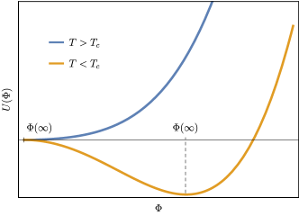
Figure 1: Profile of the effective potential $U(\Phi)$ at $r=\infty$, for $T>T_{c}$ and $T<T_{c}$, as a function of $\Phi$. The minimum of the effective potential corresponds to $\Phi(\infty)$. For $T>T_{c}$, the only possible minimum is the trivial one $\Phi(\infty)=0$.

In order to better understand the symmetry restoration we recall the effective potential $U(\Phi)$ that appears naturally in Eq. (11). We sketch in Fig. 2 the plots of $U(\Phi)$ as a function of $\Phi$ for several different radii $r$ in the case that $T_{\rm H}$ is less than $T_{c}$ at infinity. For a large radius $U(\Phi)$ as a function of $\Phi$ shows the same behavior that as at infinity, i.e., it has a local maximum and a global minimum. But, at a certain radius we have that $\braket{\phi^{2}}$ achieves a value such that the global minimum of $U(\Phi)$ in Eq. (11) is at $\Phi=0$, and so symmetry is restored, see Fig. 2. This radius we call the bubble radius $r_{\rm b}$.

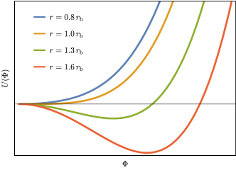
Figure 2: Sketch of the profile of the effective potential $U(\Phi)$ for decreasing radii from $r=\infty$. The minimum of the potential is negative for $r>r_{\rm b}$. From $r<r_{\rm b}$ and inwards, the minimum of the potential is zero, so the background field is $\Phi=0$ in that range.

4 Numerical solutions for Schwarzschild and Reissner-Nordström black holes

4.1 Results, plots, and analysis

In this work, we will be concerned with the spontaneously broken symmetry restoration of a scalar field around a non-charged and a charged four dimensional black hole, whose geometries are described by the Schwarzschild and Reissner-Nordström metrics, respectively, namely, $f(r)$ in Eq. (13) takes the form

$$f(r)=\left(1-\frac{r_{+}}{r}\right)\left(1-\frac{r_{-}}{r}\right)\,,$$ (29)

where $r_{+}$ is the horizon radius and $r_{-}$ the Cauchy radius. In terms of the ADM mass $m$ and electrical charge $q$ these are given by $r_{+}=m+\sqrt{m^{2}-q^{2}}$ and $r_{-}=m-\sqrt{m^{2}-q^{2}}$. For $q=0$ one $r_{+}=2m$, $r_{-}=0$ and the Schwarzschild space is recovered, $f(r)=1-\frac{r_{+}}{r}$. For $q=m$ one gets $r_{+}=r_{-}=m=q$, and the the extremal Reissner-Nordström space is obtained, $f(r)=(1-\frac{r_{+}}{r})^{2}$. We assume that $r_{+}\geq r_{-}$, i.e., $m\geq q$, so that there is always an $r_{+}$ and thus there are no naked singularities. Since for the Reissner-Nordström metric the space geometry satisfies $R=0$, the curvature coupling $\xi R$ is irrelevant. The black hole temperature is the Hawking temperature $T_{\rm H}$ given for the Reissner-Nordström space by

$$T_{\rm H}={1\over 4\pi r_{+}}\left(1-\frac{r_{-}}{r_{+}}\right)\,.$$ (30)

Schwarzschild black holes, $r_{-}=0$, are the hottest. Extremal black holes, $r_{-}=r_{+}$, are the coldest, have zero temperature. Indeed, as the Cauchy radius $r_{-}$ is increase, i.e., as the black hole electric charge increases, the black hole becomes colder, see Eq. (30).

The system of equations (15) and (16) has not an exact solution, so we must resort to an approximation scheme. To solve this system, we will employ an approximation that is self-consistent semi-classically. The procedure is as follows. First, from Eq. (24), which is a development on Eq. (16) with Eq. (19) inserted, we compute $\braket{\phi^{2}}_{\rm ren}$ for the case where no background field is present, i.e., $\Phi=0$ and so $Q(r)=\mu^{2}$, from here onwards we put $\xi R=0$. Second, we insert the result into Eq. (15) and compute the resulting $\Phi$. This step is nontrivial and will be detailed below. Third, we compute again the vacuum polarization but now with the new $\Phi$ included in Eq. (24), i.e., such that $Q(r)=\mu^{2}-3\lambda\Phi^{2}(r)$. Fourth, we take the resulting $\braket{\phi^{2}}_{\rm ren}$ and put it back into Eq. (15), giving a new function for $\Phi$. These steps are repeated until the results for the background field $\Phi$ and the vacuum polarization $\braket{\phi^{2}}_{\rm ren}$ stop changing appreciably. This is the self-consistent procedure.

We now analyze in detail the numerical procedure for solving Eq. (15). In order to solve Eq. (15) numerically, for each iteration of the self-consistent approximation, we divide the problem into three stages: First we find the bubble radius approximately, second we solve Eq. (15) from the horizon to the bubble radius, third we solve Eq. (15) from the bubble radius to infinity. The three stages spelled out are as follows. First, to find the bubble radius, for the given $\braket{\phi^{2}}_{\rm ren}$, we search from the inside by trial and error for a radius for which for the first time the effective potential shows a minimum at some nonzero $\Phi$. This gives an approximate bubble radius $r_{\rm b\,approx}$ and a field $\Phi$ at the approximate bubble radius $\Phi(r_{\rm b\,approx})$. Second, to solve Eq. (15) from the horizon to the bubble radius, i.e., inside the bubble, we choose a point very close to the horizon, essential $r_{+}$, and evaluate the minimum of the effective potential for that radius, obtaining $\Phi(r_{+})$. Using this value $\Phi(r_{+})$ together with the determined value of the background field at the approximate bubble radius $\Phi(r_{\rm b\,approx})$, we find the solution inside the bubble using Eq. (15). Third, to solve from the bubble radius to infinity, i.e., for the region outside the bubble, it remains to find the value of the field at infinity, i.e., for some sufficient large value of the radius. Since the field will be considered to be at thermal equilibrium with the black hole, its value at infinity $\Phi(\infty)$ will be given by Eq. (27) at the black hole temperature, i.e., $T_{\rm H}$, with $T_{\rm H}$ given by Eq. (30). Using this value of $\Phi(\infty)$ together with the determined value of the background field at the approximate bubble radius $\Phi(r_{\rm b\,approx})$, we find using Eq. (15) the solution outside the bubble. Thus, for a given $\braket{\phi^{2}}_{\rm ren}$ we find $\Phi(r)$ for the whole space. We then resort to the next step in the self-consistent approximation until the solution stops changing appreciably.

At this stage we have a well-defined bubble radius $r_{\rm b}$ and the solution $\Phi(r)$ and $\braket{\phi^{2}}_{\rm ren}(r)$ throughout all space. Employing thus the self-consistent approximation we obtain the results for the background field $\Phi(r)$ in Fig. 4 and for the vacuum polarization $\braket{\phi^{2}}_{\rm ren}(r)$ in Fig. 4. A careful analysis of the results and plots is now in order.

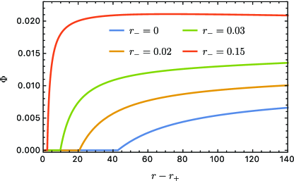
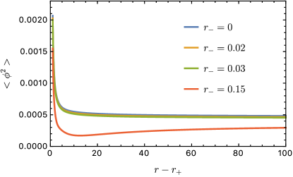
Figure 3: Profile of the background field $\Phi$ for $\lambda=7.1\times 10^{-3}$, $\mu=0.01$, $r_{+}=1$ and varying $r_{-}$. The case $r_{-}=0$ is the Schwarzschild case and $r_{-}=0.02,0.03,0.15$ are typical Reissner-Nordström cases. The extremal case $r_{-}=1$, not shown, starts from $\Phi=0$ at $r-r_{+}=0$ and jumps immediately to a finite value in a step function as can be inferred from the plots, i.e., there is no bubble for extremal black holes.

Figure 4: Profile of the vacuum polarization $\braket{\phi^{2}}_{\rm ren}$ for $\lambda=7.1\times 10^{-3}$, $\mu=0.01$, $r_{+}=1$ and varying $r_{-}$. The case $r_{-}=0$ is the Schwarzschild case and $r_{-}=0.02,0.03,0.15$ are typical Reissner-Nordström cases. The extremal case $r_{-}=1$, not shown, gives $\braket{\phi^{2}}_{\rm ren}=0$ for all $r-r_{+}$ as can be inferred from the plots, i.e., there is no vacuum polarization for extremal black holes.

From the point of view of the background field $\Phi$, spontaneously broken symmetry restoration is less likely for colder black holes, so colder black holes, i.e., more charged ones, will have a smaller bubble of restored symmetry, something that is clear from Fig. 4. For extremal black holes $r_{-}=r_{+}$ the bubble has zero width, thus for extreme black holes there is no bubble, and the curve is a step function. Although not shown it is clear that this is the limit of the curves drawn in Fig. 4.

From the point of view of the vacuum polarization $\braket{\phi^{2}}_{\rm ren}$, there are several aspects that one can rise: (i) For colder black holes it becomes harder to excite the quantum field modes, so the vacuum polarization for those black holes has smaller values as can be checked in Fig. 4 when comparing each different curve $r_{-}$. Extremal black holes $r_{-}=r_{+}$ have zero temperature, the vacuum polarization is never excited, and so the curve is the line $\braket{\phi^{2}}_{\rm ren}(r)=0$. Although not shown it is clear that this is the limit of the curves drawn in Fig. 4. (ii) For each black hole, i.e., for a given $r_{-}$, we clearly see from Fig. 4 that as $r$ increases, and thus the temperature decreases, it also becomes harder to excite the quantum field modes, so the vacuum polarization is smaller as $r$ increases. (iii) The influence of the background field $\Phi$ for a given curve $r_{-}$ at the horizon and at infinity is also worth analyzing. At the horizon, the background field $\Phi$ is negligible, so the value of $\braket{\phi(r_{+})^{2}}$ is unaltered by $\Phi$, the changes in $\braket{\phi(r_{+})^{2}}$ there come from other sources. At infinity, the field $\Phi$ has its largest value which translates into a smaller effective mass squared $Q=\mu^{2}-3\lambda\Phi^{2}$ and in turn this increases the vacuum polarization. (iv) Another interesting fact is that the overall form of the vacuum polarization is more affected by smaller bubbles. This is because $\braket{\phi^{2}}$ stabilizes quickly in a distance relatively small from the horizon, so the background field can only alter the form of the vacuum polarization curve when its region of larger variations, i.e., the outer edge of the bubble, is situated near the horizon. For larger bubbles, we see from Fig. 4 that the effects of the background field on the vacuum polarization are not so distinct.

4.2 Comments on the numerical calculations

Commenting on the numerical calculations, we observe that the solutions stabilize relatively fast, at the order of three or four iterations of the self-consistent approximation.

Regarding the vacuum polarization, the method employed here converges quickly on the horizon, where only some tens of modes are necessary to obtain a good result. However, at large radii, at the order of some hundreds of $r_{+}$, the convergence for the vacuum polarization becomes slower, requiring the sum of some hundreds of modes. Since the order of magnitude of each Green mode function becomes very small for large distances, we are faced with the task of calculating very accurately hundreds of differences between very small numbers in Eq. (24). As a consequence, we must find the numerical solutions of the homogeneous version of Eq. (21) for each mode with a very high precision, which revealed to be a considerable heavy and fine-tuned task for the symbolic manipulation software Mathematica used by us for the purpose. These shortcomings increased the overall computational time, which was reasonably lessened by parallelizing the code and using it in a cluster. In this regard, the numeric efficiency may be improved by adopting a different method to find the numerical solutions for the mode functions.

The results have been further checked using a slightly different approach which fixes the value of the field asymptotically and uses the value of the derivative as a shooting parameter. We have verified in a number of cases that the solutions obtained in the two ways coincide to the numerical accuracy we have used.

5 Conclusions

In this work we have constructed bubble solutions for a self-interacting quantum scalar field around non-charged and charged four dimensional black holes. These bubble solutions can be envisaged as solitons with $\Phi=0$ inside the bubble and $\Phi$ finite outside it. The method we have adopted includes a self-consistent calculation of one-loop quantum effects encoded in the scalar vacuum polarization. The results we have obtained clearly demonstrate the picture where a spontaneously broken symmetry phase far away from the black hole is restored sufficiently near its horizon due to the increase of the local temperature associated to the gravitational blueshift from the Hawking temperature at infinity to an large unbound temperature at the horizon. We have confirmed this picture by extending the results of Hawking:1980ng ; Fawcett:1981fw ; Moss:1984zf and by explicitly constructing the solutions for the bubble configuration. In particular, we have observed that hot black holes have large bubble regions where the temperature is high enough to induce a phase transition in the value of $\Phi$, cold black holes have small bubbles, with the extremal black hole, at zero temperature, having no bubble, $\Phi$ is a nonzero constant throughout.

Appendix: Hadamard coefficients

For a field with a radial dependent mass term squared, $Q(r)$, we find the Hadamard coefficients below. In the formulas, to avoid the appearance of $2\pi$ and its powers an excessive number of times, we use the surface gravity $\kappa$ of the black hole instead of its Hawking temperature $T_{\rm H}$, the relation between them being $T_{\rm H}={\kappa\over 2\pi}$. Denote differentiation with respect to the radial coordinate with a prime. The Hadamard coefficients are

$$\mathcal{D}^{(+)}_{00}= \,2\,,$$ (31)

$$\mathcal{D}^{(+)}_{10}= \,\frac{f}{6r^{2}}+\frac{f^{\prime}f}{6r}-\frac{1}{12}f^{\prime\prime}f-\frac{f^{2}}{6r^{2}}\,,$$ (32)

$$\mathcal{D}^{(+)}_{11}= \,-\frac{1}{6}\kappa^{2}f+\frac{1}{24}f^{\prime 2}f-\frac{f^{2}}{6r^{2}}-\frac{f^{\prime}f^{2}}{6r}+\frac{f^{3}}{6r^{2}}\,,$$ (33)

$$\mathcal{D}^{(+)}_{20}= \,\frac{\kappa^{2}f}{72r^{2}}+\frac{\kappa^{2}f^{\prime}f}{72r}-\frac{f^{\prime 2}f}{288r^{2}}-\frac{f^{\prime 3}f}{288r}-\frac{1}{144}\kappa^{2}f^{\prime\prime}f+\frac{1}{576}f^{\prime 2}f^{\prime\prime}f+\frac{f^{2}}{720r^{4}}-\frac{\kappa^{2}f^{2}}{72r^{2}}$$

$$+\frac{f^{\prime}f^{2}}{36r^{3}}+\frac{43f^{\prime 2}f^{2}}{1440r^{2}}-\frac{f^{\prime\prime}f^{2}}{144r^{2}}-\frac{7f^{\prime}f^{\prime\prime}f^{2}}{360r}+\frac{1}{320}{f^{\prime\prime}}^{2}f^{2}+\frac{1}{240}f^{\prime}f^{(3)}f^{2}-\frac{f^{3}}{36r^{4}}$$

$$-\frac{19f^{\prime}f^{3}}{360r^{3}}+\frac{7f^{\prime\prime}f^{3}}{360r^{2}}-\frac{f^{(3)}f^{3}}{120r}+\frac{19f^{4}}{720r^{4}}\,,$$ (34)

$$\mathcal{D}^{(+)}_{21}= \,-\frac{1}{45}\kappa^{4}f+\frac{1}{144}\kappa^{2}f^{\prime 2}f-\frac{f^{\prime 4}f}{2880}-\frac{\kappa^{2}f^{2}}{24r^{2}}-\frac{\kappa^{2}f^{\prime}f^{2}}{24r}+\frac{f^{\prime 2}f^{2}}{96r^{2}}+\frac{f^{\prime 3}f^{2}}{96r}+\frac{1}{144}\kappa^{2}f^{\prime\prime}f^{2}$$

$$-\frac{11f^{\prime 2}f^{\prime\prime}f^{2}}{2880}-\frac{7f^{3}}{360r^{4}}+\frac{\kappa^{2}f^{3}}{24r^{2}}-\frac{f^{\prime}f^{3}}{18r^{3}}-\frac{67f^{\prime 2}f^{3}}{1440r^{2}}+\frac{f^{\prime\prime}f^{3}}{144r^{2}}+\frac{11f^{\prime}f^{\prime\prime}f^{3}}{720r}+\frac{f^{4}}{18r^{4}}$$

$$+\frac{13f^{\prime}f^{4}}{180r^{3}}-\frac{11f^{\prime\prime}f^{4}}{720r^{2}}-\frac{13f^{5}}{360r^{4}}\,,$$ (35)

$$\mathcal{D}^{(+)}_{22}= \,\frac{1}{72}\kappa^{4}f^{2}-\frac{1}{144}\kappa^{2}f^{\prime 2}f^{2}+\frac{f^{\prime 4}f^{2}}{1152}+\frac{\kappa^{2}f^{3}}{36r^{2}}+\frac{\kappa^{2}f^{\prime}f^{3}}{36r}-\frac{f^{\prime 2}f^{3}}{144r^{2}}-\frac{f^{\prime 3}f^{3}}{144r}+\frac{f^{4}}{72r^{4}}-\frac{\kappa^{2}f^{4}}{36r^{2}}$$

$$+\frac{f^{\prime}f^{4}}{36r^{3}}+\frac{f^{\prime 2}f^{4}}{48r^{2}}-\frac{f^{5}}{36r^{4}}-\frac{f^{\prime}f^{5}}{36r^{3}}+\frac{f^{6}}{72r^{4}}\,,$$ (36)

$$\mathcal{T}^{(l)}_{00}= \,\frac{1}{24}Q\kappa^{2}f-\frac{\kappa^{2}f}{72r^{2}}+\frac{\kappa^{2}f^{\prime}f}{36r}-\frac{1}{96}Qf^{\prime 2}f+\frac{f^{\prime 2}f}{288r^{2}}-\frac{f^{\prime 3}f}{144r}+\frac{1}{144}\kappa^{2}f^{(2)}f-\frac{1}{576}f^{\prime 2}f^{(2)}f$$

$$-\frac{f^{2}}{72r^{4}}+\frac{Qf^{2}}{24r^{2}}+\frac{\kappa^{2}f^{2}}{72r^{2}}+\frac{f^{\prime}f^{2}}{72r^{3}}+\frac{Qf^{\prime}f^{2}}{24r}+\frac{7f^{\prime 2}f^{2}}{288r^{2}}+\frac{f^{(2)}f^{2}}{144r^{2}}+\frac{f^{\prime}f^{(2)}f^{2}}{144r}+\frac{f^{3}}{36r^{4}}$$

$$-\frac{Qf^{3}}{24r^{2}}-\frac{f^{\prime}f^{3}}{72r^{3}}-\frac{f^{(2)}f^{3}}{144r^{2}}-\frac{f^{4}}{72r^{4}}\,,$$ (37)

$$\mathcal{T}^{(l)}_{10}= \,\frac{Q}{2}-\frac{1}{6r^{2}}+\frac{f^{\prime}}{3r}+\frac{f^{(2)}}{12}+\frac{f}{6r^{2}}\frac{Q^{2}}{16}-\frac{1}{120r^{4}}-\frac{1}{48}Q^{\prime}f^{\prime}+\frac{Qf^{\prime}}{24r}+\frac{f^{\prime 2}}{120r^{2}}+\frac{1}{48}Qf^{(2)}$$

$$-\frac{f^{\prime}f^{(2)}}{120r}+\frac{{f^{(2)}}^{2}}{480}-\frac{1}{240}f^{\prime}f^{(3)}-\frac{1}{48}Q^{(2)}f-\frac{Q^{\prime}f}{12r}+\frac{f^{\prime}f}{40r^{3}}-\frac{f^{(2)}f}{30r^{2}}-\frac{7f^{(3)}f}{240r}$$

$$-\frac{1}{240}f^{(4)}f+\frac{f^{2}}{120r^{4}}\,,$$ (38)

$$\mathcal{T}^{(l)}_{11}= \,\frac{f}{60r^{4}}-\frac{Qf}{24r^{2}}-\frac{1}{48}Q^{\prime}f^{\prime}f-\frac{f^{\prime}f}{24r^{3}}+\frac{f^{\prime 2}f}{240r^{2}}-\frac{1}{48}Qf^{(2)}f-\frac{f^{\prime}f^{(2)}f}{40r}-\frac{1}{240}{f^{(2)}}^{2}f$$

$$-\frac{1}{480}f^{\prime}f^{(3)}f+\frac{Qf^{2}}{24r^{2}}+\frac{Q^{\prime}f^{2}}{24r}+\frac{f^{\prime}f^{2}}{30r^{3}}+\frac{f^{(2)}f^{2}}{40r^{2}}+\frac{f^{(3)}f^{2}}{80r}+\frac{1}{480}f^{(4)}f^{2}-\frac{f^{3}}{60r^{4}}\,.$$ (39)

References

- (1) I. Y. Kobzarev, L. B. Okun, and M. B. Voloshin, “Bubbles in metastable vacuum”, Sov. J. Nucl. Phys. 20, 644 (1975) [Yad. Fiz. 20, 1229 (1974)].
- (2) S. R. Coleman, “The fate of the false vacuum. 1. Semiclassical theory”, Phys. Rev. D 15, 2929 (1977); Erratum: Phys. Rev. D 16, 1248 (1977).
- (3) C. G. Callan and S. R. Coleman, “The fate of the false vacuum. 2. First quantum corrections”, Phys. Rev. D 16, 1762 (1977).
- (4) S. R. Coleman and F. de Luccia, “Gravitational effects on and of vacuum decay”, Phys. Rev. D 21, 3305 (1980).
- (5) CMS collaboration, “Combined results of searches for the standard model Higgs boson in pp collisions at TeV”, Phys. Lett. B710, 26 (2012); arXiv:1202.1488 [hep-ex].
- (6) ATLAS collaboration, “Combined search for the Standard Model Higgs boson using up to 4.9 fb-1 of pp collision data at TeV with the ATLAS detector at the LHC”, Phys. Lett. B710, 49 (2012); arXiv:1202.1408 [hep-ex].
- (7) G. Degrassi, S. Di Vita, J. Elias-Miró, J. R. Espinosa, G. F. Giudice, G. Isidori, and A. Strumia, “Higgs mass and vacuum stability in the Standard Model at NNLO”, J. High Energ. Phys. JHEP 08 (2012) 098; arXiv:1205.6497 [hep-ph].
- (8) J. R. Espinosa, G. F. Giudice, E. Morgante, A. Riotto, L. Senatore, A. Strumia, and N. Tetradis, “The cosmological Higgstory of the vacuum instability”, J. High Energ. Phys. JHEP 09 (2015) 174; arXiv:1505.04825 [hep-ph].
- (9) V. Branchina, E. Messina, and M. Sher, “Lifetime of the electroweak vacuum and sensitivity to Planck scale physics”, Phys. Rev. D 91, 013003 (2015); arXiv:1408.5302 [hep-ph].
- (10) S. W. Hawking, “Interacting quantum fields around a black hole”, Commun. Math. Phys. 80, 421 (1981).
- (11) M. S. Fawcett and B. F. Whiting “Spontaneous symmetry breaking near a black hole”, in Quantum Structure of Space and Time, Nuffield Workshop, London 1981, editors: M. J. Duff and C. J. Isham (Cambridge University Press, Cambridge 1982), p. 131.
- (12) I. G. Moss, “Black hole bubbles”, Phys. Rev. D 32, 1333 (1985).
- (13) W. A. Hiscock, “Can black holes nucleate vacuum phase transitions?”, Phys. Rev. D 35, 1161 (1987).
- (14) S. Benić and A. Yamamoto, “Quantum Monte Carlo simulation with a black hole”, Phys. Rev. D 93, 094505 (2016); arXiv:1603.00716 [hep-lat].
- (15) A. Flachi and T. Tanaka, “Chiral phase transitions around black holes”, Phys. Rev. D 84 061503 (2011); arXiv:1106.3991 [hep-th].
- (16) A. Flachi and T. Tanaka, “Chiral modulations in curved space I: Formalism”, J. High Energ. Phys JHEP 02 (2011) 026; arXiv:1012.0463 [hep-th]
- (17) A. Flachi, “Black holes as QCD laboratories”, Int. J. Mod. Phys. D 24, 1542017 (2015).
- (18) R. Gregory, I. G. Moss, and B. Withers, “Black holes as bubble nucleation sites”, J. High Energ. Phys JHEP 03 (2014) 081; arXiv:1401.0017 [hep-th].
- (19) P. Burda, R. Gregory, and I. Moss, “Vacuum metastability with black holes”, J. High Energ. Phys JHEP 08 (2015) 114; arXiv:1503.07331 [hep-th].
- (20) P. Burda, R. Gregory, and I. Moss, “The fate of the Higgs vacuum”, J. High Energ. Phys JHEP 06 (2016) 025; arXiv:1601.02152 [hep-th].
- (21) A. Flachi and K. Fukushima, “Chiral mass-gap in curved space”, Phys. Rev. Lett. 113, 091102 (2014); arXiv:1406.6548 [hep-th].
- (22) E. V. Castro, A. Flachi, P. Ribeiro, and V. Vitagliano, “Symmetry breaking and lattice kirigami”, Phys. Rev. Lett. 121, 221601 (2018); arXiv:1803.09495 [hep-th].
- (23) L. E. Parker and D. Toms, Quantum Field Theory in Curved Spacetime (Cambridge University Press, Cambridge, 2009).
- (24) P. Candelas, “Vacuum polarization in Schwarzschild space-time”, Phys. Rev. D 21, 2185 (1980).
- (25) P. R. Anderson, “ for massive fields in Schwarzschild space-time”, Phys. Rev. D 39, 3785 (1989).
- (26) P. Taylor and C. Breen, “Mode-sum prescription for vacuum polarization in black hole spacetimes in even dimensions”, Phys. Rev. D 96, 105020 (2017); arXiv:1709.00316 [gr-qc]
- (27) M. Hewitt, Vacuum Polarisation on Higher Dimensional Black Hole Spacetimes, Ph.D. thesis (University of Sheffield, 2015).